Novel Function Approximation Techniques for Large-scale ...

Novel Function Approximation Techniques for

Large-scale Reinforcement Learning

A Dissertation

by

Cheng Wu

to

the Graduate School of Engineering

in Partial Fulfillment of the Requirements

for the Degree of

Doctor of Philosophy

in the field of

Computer Engineering

Advisor: Prof. Waleed Meleis

Northeastern University

Boston, Massachusetts

April 2010 in which submitted to GPO

c© Copyright May 2010 conferred by Cheng Wu

All Rights Reserved

ii

NORTHEASTERN UNIVERSITY

Graduate School of Engineering

Thesis Title: Novel Function Approximation Techniques for Large-scale Reinforcement

Learning.

Author: Cheng Wu.

Program: Computer Engineering

Approved for Dissertation Requirements of the Doctor of Philosophy Degree:

Thesis Advisor: Waleed Meleis Date

Thesis Reader: Jennifer Dy Date

Thesis Reader: Javed A. Aslam Date

Chairman of Department: Date

Graduate School Notified of Acceptance:

Director of the Graduate School: Date

iii

Contents

1 Introduction 1

1.1 Reinforcement Learning . . . . . . . . . . . . . . . . . . . . . . . . . . . . . 3

1.2 Function Approximation . . . . . . . . . . . . . . . . . . . . . . . . . . . . . 5

1.2.1 Function Approximation Using Natural Features . . . . . . . . . . . . 8

1.2.2 Function Approximation Using Basis Functions . . . . . . . . . . . . 10

1.2.3 Function Approximation Using SDM . . . . . . . . . . . . . . . . . . 12

1.3 Our Application Domain . . . . . . . . . . . . . . . . . . . . . . . . . . . . . 13

1.4 Dissertation Outline . . . . . . . . . . . . . . . . . . . . . . . . . . . . . . . 15

2 Adaptive Function Approximation 19

2.1 Experimental Evaluation: Traditional Function Approximation . . . . . . . . 20

2.1.1 Application Instances . . . . . . . . . . . . . . . . . . . . . . . . . . . 20

2.1.2 Performance Evaluation of Traditional Tile Coding . . . . . . . . . . 22

2.1.3 Performance Evaluation of Traditional Kanerva Coding . . . . . . . . 25

2.2 Visit Frequency and Feature Distribution . . . . . . . . . . . . . . . . . . . . 28

iv

2.3 Adaptive Mechanism in Kanerva-Based Function Approximation . . . . . . . 31

2.3.1 Prototype Deletion and Generation . . . . . . . . . . . . . . . . . . . 32

2.3.2 Performance Evaluation of Adaptive Kanerva-Based Function Approx-

imation . . . . . . . . . . . . . . . . . . . . . . . . . . . . . . . . . . 34

2.4 Summary . . . . . . . . . . . . . . . . . . . . . . . . . . . . . . . . . . . . . 37

3 Fuzzy Logic-based Function Approximation 38

3.1 Experimental Evaluation: Kanerva Coding Applied to Hard Instances . . . . 39

3.2 Prototype Collisions in Kanerva Coding . . . . . . . . . . . . . . . . . . . . 41

3.3 Adaptive Fuzzy Kanerva Coding . . . . . . . . . . . . . . . . . . . . . . . . . 48

3.3.1 Fuzzy and Adaptive Mechanism . . . . . . . . . . . . . . . . . . . . . 49

3.3.2 Adaptive Fuzzy Kanerva Coding Algorithm . . . . . . . . . . . . . . 51

3.3.3 Performance Evaluation of Adaptive Fuzzy Kanerva-Based Function

Approximation . . . . . . . . . . . . . . . . . . . . . . . . . . . . . . 53

3.4 Prototype Tuning . . . . . . . . . . . . . . . . . . . . . . . . . . . . . . . . . 55

3.4.1 Experimental Evaluation: Similarity Analysis of Membership Vectors 55

3.4.2 Tuning Mechanism . . . . . . . . . . . . . . . . . . . . . . . . . . . . 58

3.4.3 Performance Evaluation of Tuning Mechanism . . . . . . . . . . . . . 58

3.5 Summary . . . . . . . . . . . . . . . . . . . . . . . . . . . . . . . . . . . . . 61

4 Rough Sets-based Function Approximation 63

4.1 Experimental Evaluation: Effect of Varying Number of Prototypes . . . . . . 64

v

4.2 Rough Sets and Kanerva Coding . . . . . . . . . . . . . . . . . . . . . . . . 66

4.3 Rough Sets-based Kanerva Coding . . . . . . . . . . . . . . . . . . . . . . . 71

4.3.1 Prototype Deletion and Generation . . . . . . . . . . . . . . . . . . . 73

4.3.2 Rough Sets-based Kanerva Coding Algorithm . . . . . . . . . . . . . 74

4.3.3 Performance Evaluation of Rough Sets-based Kanerva Coding . . . . 77

4.4 Effect of Varying the Number of Initial Prototypes . . . . . . . . . . . . . . 81

4.5 Summary . . . . . . . . . . . . . . . . . . . . . . . . . . . . . . . . . . . . . 83

5 Real-world Application: Cognitive Radio Network 84

5.1 Introduction . . . . . . . . . . . . . . . . . . . . . . . . . . . . . . . . . . . . 84

5.2 Reinforcement Learning-Based Cognitive Radio . . . . . . . . . . . . . . . . 88

5.2.1 Problem Formulation . . . . . . . . . . . . . . . . . . . . . . . . . . . 88

5.2.2 Application to cognitive radio . . . . . . . . . . . . . . . . . . . . . . 89

5.3 Experimental Simulation . . . . . . . . . . . . . . . . . . . . . . . . . . . . . 94

5.3.1 Simulation Setup . . . . . . . . . . . . . . . . . . . . . . . . . . . . . 94

5.3.2 Simulation Evaluation . . . . . . . . . . . . . . . . . . . . . . . . . . 97

5.4 Function Approximation for RL-based Cognitive Radio . . . . . . . . . . . . 102

5.5 Summary . . . . . . . . . . . . . . . . . . . . . . . . . . . . . . . . . . . . . 104

6 Conclusion 106

Bibliography 111

vi

List of Figures

2.1 The grid world of size 32 x 32. . . . . . . . . . . . . . . . . . . . . . . . . . . 21

2.2 The implementation of the tiling. . . . . . . . . . . . . . . . . . . . . . . . . 23

2.3 The fraction of test instances solved by Q-Learning with traditional Tile Cod-

ing with 2000 tiles. . . . . . . . . . . . . . . . . . . . . . . . . . . . . . . . . 24

2.4 The implementation of Kanerva Coding. . . . . . . . . . . . . . . . . . . . . 25

2.5 The fraction of test instances solved by Q-Learning with traditional Kanerva

Coding with 2000 prototypes. . . . . . . . . . . . . . . . . . . . . . . . . . . 27

2.6 The frequency distribution of visits to tiles over a sample run using Q-learning

with Tile Coding . . . . . . . . . . . . . . . . . . . . . . . . . . . . . . . . . 30

2.7 The frequency distribution of visits to prototypes over a sample run using

Q-learning with Kanerva Coding . . . . . . . . . . . . . . . . . . . . . . . . . 30

2.8 The fraction of test instances solved by Q-Learning with adaptive Kanerva

Coding with 2000 prototypes. . . . . . . . . . . . . . . . . . . . . . . . . . . 35

2.9 The frequency distribution of visits to prototypes over a sample run using

Q-learning with adaptive Kanerva Coding. . . . . . . . . . . . . . . . . . . . 36

vii

3.1 The fraction of easy and hard test instances solved by Q-learning with adaptive

Kanerva Coding with 2000 prototypes. . . . . . . . . . . . . . . . . . . . . . 41

3.2 The illustration of prototype collision. (a) adjacent to no prototype; (b) ad-

jacent to an identical prototype set; (c) adjacent to unique prototype vectors. 42

3.3 Prototype collisions using traditional and adaptive Kanerva-based function

approximation with 2000 prototypes. . . . . . . . . . . . . . . . . . . . . . . 44

3.4 Average fraction of test instances solved (solution rate) (a) 8x8 grid; (c) 16x16

grid; (e) 32x32 grid, and the fraction of of state-action pairs that are adjacent

to no prototypes and adjacent to identical prototype vectors (collision rate) (b)

8x8 grid; (d) 16x16 grid; (f) 32x32 grid by traditional and adaptive Kanerva-

based function approximation as the number of prototypes varies from 300 to

2500. . . . . . . . . . . . . . . . . . . . . . . . . . . . . . . . . . . . . . . . . 46

3.5 Sample membership function for traditional Kanerva Coding. . . . . . . . . . 49

3.6 Sample membership function for fuzzy Kanerva Coding. . . . . . . . . . . . . 50

3.7 Average solution rate for adaptive fuzzy Kanerva Coding with 2000 prototypes. 54

3.8 (a) Distribution of membership grades and (b) prototype similarity across

sorted prototypes. . . . . . . . . . . . . . . . . . . . . . . . . . . . . . . . . . 56

3.9 Illustration of the similarity of membership vectors across sparse and dense

prototype regions. . . . . . . . . . . . . . . . . . . . . . . . . . . . . . . . . . 57

3.10 Average solution rate for adaptive fuzzy Kanerva Coding with Tuning using

2000 prototypes. . . . . . . . . . . . . . . . . . . . . . . . . . . . . . . . . . 59

viii

3.11 The four-room gridworld . . . . . . . . . . . . . . . . . . . . . . . . . . . . . 60

3.12 Average solution rate for adaptive Fuzzy Kanerva Coding with Tuning in the

four-room gridworld of size 32x32. . . . . . . . . . . . . . . . . . . . . . . . . 61

4.1 The fraction of hard test instances solved by Q-learning with adaptive Kanerva

Coding as the number of prototypes decreases. . . . . . . . . . . . . . . . . . 66

4.2 Illustration of equivalence classes of the sample. . . . . . . . . . . . . . . . . 68

4.3 The fraction of equivalence classes that contain two or more state-action pairs

over all equivalence classes, the conflict rate, and its corresponding solution

rate and collision rate using traditional Kanerva and adaptive Kanerva with

frequency-based prototype optimization across all sizes of grids . . . . . . . . 70

4.4 The fraction of prototypes remaining after performing a prototype reduct

using traditional and optimized Kanerva-based function approximation with

2000 prototypes. The original and final number of prototypes is shown on

each bar. . . . . . . . . . . . . . . . . . . . . . . . . . . . . . . . . . . . . . . 72

4.5 Average solution rate for traditional Kanerva, adaptive Kanerva and rough

sets-based Kanerva (a), in 8x8 grid; (b), in 16x16 grid; (c), in 32x32 grid. . . 78

4.6 Effect of rough sets-based Kanerva on the number of prototypes and the frac-

tion of equivalence classes (a), in 8x8 grid; (b), in 16x16 grid; (c), in 32x32

grid. . . . . . . . . . . . . . . . . . . . . . . . . . . . . . . . . . . . . . . . . 80

4.7 Variation in the number of prototypes with different numbers of initial proto-

types with rough sets-based Kanerva in a 16x16 grid. . . . . . . . . . . . . . 82

ix

5.1 The CR ad hoc architecture . . . . . . . . . . . . . . . . . . . . . . . . . . . 86

5.2 The cognitive radio cycle for the CR ad hoc architecture . . . . . . . . . . . 87

5.3 Multi-agent reinforcement learning based cognitive radio. . . . . . . . . . . . 90

5.4 Comparative reward levels for different observed scenarios . . . . . . . . . . 92

5.5 Block diagram of the implemented simulator tool for reinforcement learning

based cognitive radio. . . . . . . . . . . . . . . . . . . . . . . . . . . . . . . . 94

5.6 The performance of small topology. . . . . . . . . . . . . . . . . . . . . . . . 98

5.7 The performance of the real-world topology with five different node densities. 100

5.8 Average probability of successful transmission for the real-world topology with

500 nodes. . . . . . . . . . . . . . . . . . . . . . . . . . . . . . . . . . . . . . 103

x

List of Tables

2.1 The average fraction of test instances solved by Q-learning with traditional

Tile Coding. . . . . . . . . . . . . . . . . . . . . . . . . . . . . . . . . . . . . 24

2.2 The average fraction of test instances solved by Q-learning with traditional

Kanerva Coding. . . . . . . . . . . . . . . . . . . . . . . . . . . . . . . . . . 26

2.3 The average fraction of test instances solved by Q-learning with adaptive

Kanerva Coding. . . . . . . . . . . . . . . . . . . . . . . . . . . . . . . . . . 34

3.1 The average fraction of test instances solved by Q-learning with adaptive

Kanerva Coding. . . . . . . . . . . . . . . . . . . . . . . . . . . . . . . . . . 40

3.2 The average fraction of test instances solved by Q-Learning with adaptive

fuzzy Kanerva Coding. . . . . . . . . . . . . . . . . . . . . . . . . . . . . . . 53

4.1 The average fraction of test instances solved by Q-Learning with adaptive

Kanerva Coding. . . . . . . . . . . . . . . . . . . . . . . . . . . . . . . . . . 65

4.2 Sample of adjacency between state-action pairs and prototypes. . . . . . . . 67

xi

4.3 Percentage improved performance of rough sets-based Kanerva over adaptive

Kanerva. . . . . . . . . . . . . . . . . . . . . . . . . . . . . . . . . . . . . . . 79

xii

Abstract

Function approximation can be used to improve the performance of reinforcement learn-

ers. Traditional techniques, including Tile Coding and Kanerva Coding, can give poor

performance when applied to large-scale problems. In our preliminary work, we show that

this poor performance is caused by prototype collisions and uneven prototype visit frequency

distributions. We describe our adaptive Kanerva-based function approximation algorithm,

based on dynamic prototype allocation and adaptation. We show that probabilistic proto-

type deletion with prototype splitting can make the distribution of visit frequencies more

uniform, and that dynamic prototype allocation and adaptation can reduce prototoype coll-

sisions. This approach can significantly improve the performance of a reinforcement learner.

We then show that fuzzy Kanerva-based function approximation can reduce the similarity

between the membership vectors of state-action pairs, giving even better results. We use

Maximum Likelihood Estimation to adjust the variances of basis functions and tune the

receptive fields of prototypes. This approach completely eliminates prototype collisions, and

greatly improve the ability of a Kanerva-based reinforcement learner to solve large-scale

problems.

Since the number of prototypes remains hard to select, we describe a more effective

approach for adaptively selecting the number of prototypes. Our new rough sets-based

Kanerva-based function approximation uses rough sets theory to explain how prototype

2

collisions occur. Our algorithm eliminates unnecessary prototypes by replacing the original

prototype set with its reduct, and reduces prototype collisions by splitting equivalence classes

with two or more state-action pairs. The approach can adaptively select an effective number

of prototypes and greatly improve a Kanerva-based reinforcement learners ability.

Finally, we apply function approximation techniques to scale up the ability of reinforce-

ment learners to solve a real-world application: spectrum management in cognitive radio

networks. We use multi-agent reinforcement learning approach with decentralized control

can be used to select transmission parameters and enable efficient assignment of spectrum

and transmit powers. However, the requirement of RL-based approaches that an estimated

value be stored for every state greatly limits the size and complexity of CR networks that

can be solved. We show that function approximation can reduce the memory used for large

networks with little loss of performance. We conclude that our spectrum management ap-

proach based on reinforcement learning with Kanerva-based function approximation can

significantly reduce interference to licensed users, while maintaining a high probability of

successful transmissions in a cognitive radio ad hoc network.

Chapter 1

Introduction

Machine learning, a field of artificial intelligence, can be used to solve search problems using

prior knowledge, known experience and data. Many powerful computational and statistical

paradigms have been developed, including supervised learning, unsupervised learning, trial-

and-error learning and reinforcement learning.

However, machine learning techniques can struggle to solve large-scale problems with huge

state and action spaces [12]. Various solutions to this problem under have been studied, such

as dimensionality reduction [2], principle component analysis [22], support vector machines

[14], and function approximation [17].

Reinforcement learning, one of the most successful machine learning paradigms, enables

learning from feedback received through interactions with an external environment. Like the

other paradigms for machine learning, a key drawback of reinforcement learning is that it

only works well for small problems, and performs poorly for large-scale problems [43].

1

CHAPTER 1. INTRODUCTION 2

Function approximation [17, 40] is a technique for resolving this problem within the

context of reinforcement learning. Instead of using a look-up table to directly store values

of points within the state and action space, it uses examples of the desired value function to

reconstruct an approximation of this function and compute an estimate of the desired value

from the approximation function.

When using many function approximation techniques, a complex parametric approxima-

tion architecture is used to compute good estimates of the desired value function [34]. An

approximation architecture is a computational structure that uses parametric functions to

approximate the value of a state or state-action pair. Using a simple approximation ar-

chitecture design often make estimates diverge from the desired value function, and makes

agents perform inefficiently [10]. Unfortunately, a complex parametric architecture may also

greatly increase the computational complexity of the function approximator itself [11].

Furthermore, large-scale problems can remain hard to solve in practice, even when the

complex architecture is applied. The key to a successful function approximator is not only

the choice of the parametric approximation architecture, but also the choices of various

control parameters under this architecture. Until recently, these choices were typically made

manually, based only on the designer’s intuition [11, 27].

In this dissertation we address the issue of solving large-scale, high-dimension prob-

lems using reinforcement learning with function approximation. We propose to develop a

novel parametric approximation architecture and corresponding parameter-tuning methods

for achieving better learning performance. This framework should satisfy several criteria: (1)


it should give accurate approximation, (2) the approximation should be local, that is, appro-

priate for a specific learning problem, (3) the parameters should be selected automatically,

and (4) it should learn online.

We first review related work on reinforcement learning and function approximation, de-

scribe their characteristics and limitations, and give examples of their operation.

1.1 Reinforcement Learning

Reinforcement learning is inspired by psychological learning theory from biology [46]. The

general idea is that within an environment, a learning agent attempts to perform optimal

actions to maximize long-term rewards achieved by interacting with the environment. An

environment is a model of a specific problem domain, typically formulated as a Markov

Decision Process (MDP) [32]. A state is some information that an agent can perceive within

the environment. An action is the behavior of an agent at a specific time at a specific state.

A reward is a measure of the desirability of an agent’s action at a specific state within the

environment.

The classic reinforcement learning algorithm is formulated as follows. At each time

t, the agent perceives its current state st ∈ S and the set of possible actions Ast . The

agent chooses an action a ∈ Ast and receives from the environment a new state st+1 and

a reward rt+1. Based on these interactions, the reinforcement learning agent must develop

a policy π : S → A which maximizes the long-term reward R =∑

t γrt for MDPs, where

0 ≤ γ ≤ 1 is a discounting factor for subsequent rewards. The long-term reward is the


expected accumulated reward for the policy.

This implementation of reinforcement learning embodies three important characteris-

tics: a human-like learning framework, the concept of a value function, and online learning.

These three characteristics distinguish reinforcement learning from other machine learning

paradigms, but they can also limit its effectiveness.

The human-like framework defines the interaction between agents and the external en-

vironment in terms of states, actions and rewards, which allows reinforcement learning to

solve the types of problems solved by humans. These types of problems tend to involve a

very large number of states and actions. Unfortunately, the performance of reinforcement

learning is very sensitive to the number of states and actions.

A value function is a function which specifies the accumulated rewards that an agent

expects to receive in the future. While a reward determines the immediate and short-term

value of an action in the current state, a value function gives the expected accumulated and

long-term value of an action under subsequent states.

The concept of a value function distinguishes reinforcement learning from evolutionary

methods [9, 7, 15]. Instead of directly searching the entire policy space by evolutionary

evaluation, a value function evaluates an action’s desirability at the current state by accu-

mulating delayed rewards. In reinforcement learning, the accuracy and efficiency of a value

function is closely related to the performance of a reinforcement learner.

In an online learning system, learning and the evaluation of the learning system occur

concurrently. However, in order to maintain this concurrency, a reinforcement learner must


compute the value of a state-action pair as fast as possible. For a large state-action space,

storing the state-action values may require a large amount of memory that may not be

available. Reducing the size of this table is therefore necessary.

One of the most successful reinforcement learning algorithm is Q-learning [47]. This

approach uses a simple value iteration update process. At time t, for each state st and each

action at, the algorithm calculates an update to its expected discounted reward, Q(st, at) as

follows:

Q(st, at)← Q(st, at) + αt(st, at)[rt + γmaxaQ(st+1, a)−Q(st, at)]

where rt is an immediate reward at time t, αt(s, a) is the learning rate such that 0 ≤ αt(s, a) ≤

1, and γ is the discount factor such that 0 ≤ γ < 1. Q-learning stores the state-action values

in a table.

The requirement that an estimated value be stored for every state-action pair limits the

size and complexity of the learning problems that can be solved. The Q-learning table is typ-

ically large because of the high dimensionality of the state-action space, or because the state

or action space is continuous. Function approximation [10], which stores an approximation

of the entire table, is one way to solve this problem.

1.2 Function Approximation

Most reinforcement learners use a tabular representation of value functions where the value

of each state or each state-action pair is stored in a table. However, for many practical

applications that have continuous state space, or very large and high-dimension discrete


state and action spaces, this approach is not feasible.

There are two explanations for this infeasibility. First, a tabular representation can only

be used to solve tasks with a small number of states and actions. The difficulty derives

both from the memory needed to store large tables, and the time and data needed to fill

the tables accurately [40]. Second, most exact state-action pairs encountered may not have

been previously encountered. Since there are often no state-action values that can be used to

distinguish actions, the only way to learn in these problems is to generalize from previously

encountered state-action pairs to pairs that have never been visited before. We must consider

how to use a limited state-action subspace to approximate a large state-action space.

Function approximation has been widely used to solve reinforcement learning problems

with large state and action spaces [20, 17, 34]. In general, function approximation defines an

approximation method which interpolates the values of unvisited points in the search space

using known values at neighboring points. Within a reinforcement learner, function approx-

imation generalizes the function values of state-action pairs that have not been previously

visited from known function values of neighboring state-action pairs.

A typical implementation of function approximation uses linear gradient descent [45]. In

this method, the approximate value function of state-action pair sa, denoted V (sa), is a

linear function of the parameter vector, denoted ~θ. The approximate value function is then

V (sa) = ~θT ~φsa =n∑i=1

θ(i)φsa(i),

where ~φsa = (φsa(1), φsa(2), ..., φsa(n)) is a vector of features with the same number of el-

ements as ~θ. This approximation can also be seen as a projection of the multidimensional


state-action space to a feature space with few dimensions. The parameter vector is a vector

with real-valued elements, ~θ = (θ(1), θ(2), ..., θ(n)), and V (s) is a smooth differentiable func-

tion of ~θ for all state-action pairs sa ∈ SA. We assume that at each step t, we observe a new

state-action pair sat with reward vt. The parameter vector is adjusted by a small amount in

the direction that would most reduce the MSE error for that state-action pair:

~θt+1 = ~θt + α[vt − V (sat)]∇~θtV (sat),

where α is a positive step-size parameter, and ∇~θtV (sat) is the vector of partial derivatives,

(∂V (sat)∂θt(1)

, ∂V (sat)∂θt(2)

, ..., ∂V (sat)∂θt(n)

). This derivative vector is the gradient of V (sat) with respect to

~θt. An advantage of this approach is that the change in ~θt is proportional to the gradient of

the MSE error of the encountered state-action pair, the direction in which the error decreases

most rapidly.

This implementation of function approximation has two important characteristics that

affect its behavior. First, the approximate value function is a linear function of these features,

and the choice of features has a direct effect on the accuracy of the approximate represen-

tation. Within the context of reinforcement learning, a state-action pair that has not been

previously encountered can be generalized from these pre-selected features. However, the

great diversity of potential types of features can make feature selection difficult.

Second, the approximate value function is actually a projection from the large target

space to a limited feature space, and the completeness of the projection depends on the

shape and size of the receptive regions of the features. Within the context of reinforcement

learning, a large state-action space can be spanned by the receptive regions of a set of features.


Features with large regions can give wide generalization, but might make the representation

of the approximation function coarser and perform only rough discrimination. Features with

small regions can give narrow generalization, but might cause many states to be out of the

receptive regions of all features. Selecting the shape and size of the receptive regions is often

difficult for particular application domains.

A range of function approximation techniques has been studied in recent years. These

techniques can be partitioned into three types, according to the two characteristics described

above: function approximation using natural features, function approximation using basis

functions, and function approximation using Sparse Distribution Memory (SDM).

1.2.1 Function Approximation Using Natural Features

For each application domain, there are natural features that can describe a state. For

example, in some pursuit problems in the grid world, we might have features for location,

vision scale, memory size, communication mechanisms, etc. Choosing such natural features

as the components of the feature vector is an important way to add prior knowledge to a

function approximator.

In function approximation using natural features, the θ-value of a feature indicates

whether the feature is present. The θ-value is constant across the features’ receptive re-

gion and falls sharply to zero at the boundary. These receptive regions may be overlapped.

A large region may give a wide but coarse generalization while a small region may give a

narrow but fine generalization.


The advantage of function approximation using natural features is that the representa-

tion of the approximate function is simple and easy to understand. The natural features

can be selected manually and their receptive regions can be adjusted based on the designer’s

intuition. A limitation of this function approximation technique is that it cannot handle

continuous state-action spaces or state-action spaces with high dimensionality. For natural-

feature-based function approximation techniques, the number of features has the largest

effect on the discrimination ability of the approximate function. Increasing the number of

features gives finer discrimination of the state-action space, but may also increase the com-

putational complexity of the algorithm. In general, more features are needed to accurately

approximate continuous state-action spaces and state-action spaces with high dimensionality,

and the number of these needed features grows exponentially with the number of dimensions

in the state-action space [34].

A typical function approximation technique using natural features is Tile Coding [6]. This

approach, which is an extension of coarse coding [20], is also known as ”Cerebellar Model

Articulator Controller,” or CMAC [6]. In Tile Coding, k tilings are selected, each of which

partitions the state-action space into tiles. The receptive field of each feature corresponds

to a tile, and a θ-value is maintained for each tile. A state-action pair p is adjacent to a

tile if the receptive field of the tile includes p. The Q-value of a state-action pair is equal

to the sum of the θ-values of all adjacent tiles. In binary Tile Coding, which is used when

the state-action space consists of discrete values, each tiling corresponds to a subset of the

bit positions in the state-action space and each tile corresponds to an assignment of binary


values to the selected bit positions.

1.2.2 Function Approximation Using Basis Functions

For certain problems, a more accurate approximation is obtained if θ-values can vary contin-

uously and represent the degree to which a feature is present. A basis function can be used to

compute such continuously varying θ-values. Basis functions can be designed manually and

the approximate value function is a function of these basis functions. In this case, function

approximation uses basis functions to evaluate the presence of every feature, then linearly

weights these values.

In function approximation with basis functions, the receptive region of a feature depends

on the parameters of the basis function of that feature. These parameters can control the

size, shape and intensity of the receptive region. In general, the θ-value of a feature can vary

across the feature’s receptive region.

An advantage of function approximation with basis function is that the approximated

function is continuous and flexible. The basis functions, each with its own parameters,

give a more precise representation of the value function across the entire state-action space.

However there are two limitations of this function approximation technique. The first is that

selecting these basis functions parameters is difficult in general [38, 17, 34]. The coefficients

of the function combination are often learned by training the solver using test instances,

while the parameters of the basis functions themselves are tuned manually. [34]. When the

number of dimensions of the state and action space is very large, such manual tuning can


be difficult.

The second difficulty is that basis function cannot handle state-action spaces with high

dimensionality. It has been found to be hard to apply to continuous problems with more

than 10 − 12 dimensions because of the difficulty of manually tuning the basic functions

[31, 25]. Also, the number of basis functions needed to approximate a state-action space can

be exponential in the number of dimensions, causing the number of basis functions needed

to be very large for a state-action space with high dimensionality.

A typical function approximation technique using basis function is Radial Base Function

Networks (RBFNs) [38]. In an RBFN, a sequence of Gaussian curves is selected as the basis

functions of the features. Each basis function ~φi for a feature i has a center ci, and width

σi. Given an arbitrary state-action pair s, the Q-value of the state-action pair with respect

to the feature i is:

φi(s) = e−||s−ci||

2

2σ2 .

The total Q-value of the state-action pair with respect to all features is the sum of the values

of φi(s) across all features.

A radial basis function is actually a real-valued function whose value depends only on

the distance from its center. It also can be considered a fuzzy membership function, and

in this sense RBFNs represent a fuzzy function approximation technique. But RBFNs are

the natural generalization of coarse coding with binary features to continuous features. A

typical RBF feature unavoidably represents information about some, but not all, dimensions

of the state-action space. This limits RBFNs from approximating large-scale, high-dimension


state-action spaces efficiently.

1.2.3 Function Approximation Using SDM

Function approximation using either natural features or basis functions is known to not scale

well for large problem domains, or to require prior knowledge [39, 38, 25]. This approach

is not well-suited to problem domains with high dimensionality. We instead seek a class of

features that can construct approximation functions without restricting the dimensionality

of the state and action space. The theory of Spare Distributed Memory (SDM) [23] gives

such a class of features. These features are often not natural features. They are typically a

set of state-action pairs chosen from the entire state and action space.

In function approximation using SDM, each receptive region is typically defined using

a distance threshold with respect to the location of the feature in the state-action space.

The θ-value of a state-action pair with respect to a feature is constant within the feature’s

receptive region, and is zero outside of this region.

An advantage of function approximation using SDM structure is that its structure is

particularly well-suited to problem domains with high dimensionality. Its computational

complexity depends entirely on the number of prototypes, which is not a function of the

number of the dimensions of the state-action space.

A limitation of this technique is that more prototypes are needed to approximate state-

action spaces for complex problem domains, and the efficiency of function approximation

using SDM is sensitive to the number of the prototypes [25]. Even when enough prototypes


are used, the performance of the reinforcement learner with SDM is often poor and unstable

[38, 26, 34]. There is no known mechanism to guarantee the convergence of the algorithm.

Kanerva Coding [24] is the implementation of SDM in function approximation for rein-

forcement learning. Here, a collection of prototype state-action pairs (prototypes), is selected,

each of which corresponds to a binary feature. A state-action pair and a prototype are said

to be adjacent if their bit-wise representations differ by no more than a threshold number

of bits. A state-action pair is represented as a collection of binary features, each of which

equals 1 if and only if the corresponding prototype is adjacent. A value θ(i) is maintained

for each prototype, and an approximation of the value of a state-action pair is then the sum

of the θ-values of the adjacent prototypes. In this way, Kanerva Coding can greatly reduce

the size of the value table that needs to be stored.

1.3 Our Application Domain

In the dissertation, we apply our study to solve the instances from two application domain.

These two domains are predator-prey pursuit domain and cognitive radio network.

The predator-prey pursuit domain [28], introduced in 1986, is a classic example of a

multi-agent system. Problems based on this domain have been solved using a wide variety

of approaches [19, 42, 3, 21] and it also has many different versions that can be used to

illustrate different multi-agent scenarios [34, 36, 37].

A general version of the predator-prey pursuit domain takes place on a rectangular grid

with one or more predator agents and one or more prey agents. Each grid cell is either open


or closed, and an agent can only occupy open cells. Each agent has an initial position. The

problem is played in a sequence of time periods. In each time period, each agent can move

to a neighboring open cell one horizontal or vertical step from its current location, or it can

remain in its current cell. All moves are assumed to occur simultaneously, and more than

one predator agent may not occupy the same cell at the same time. The goal of the predator

agents is to capture the prey agents in the shortest time.

The domain can be fully specified by selecting different numbers of predators and prey,

defining capture in different ways, and setting each agent’s visible range. The pursuit domain

is usually studied with two or more predators and one prey; capture occurs when a predator

agent is in the same cell as a prey agent or all predator agents surround a prey agent; the

agent’s visible range may be global or local (limited).

Pursuit problems are difficult to solve in general and problems similar to ours have

been proven to be NP-Complete [8, 33]. Researchers have used approaches such as genetic

algorithms [19] and reinforcement learning [42] to develop solutions. Closed-form solutions

to restricted versions of the problem have been found [3, 21], but most such problems remain

open.

The cognitive radio network domain [30], introduced in 1999, is a novel paradigm of

wireless communication. The basic idea is that the unlicensed devices (also called cognitive

radio users) need to vacate the band once the licensed devices (also known as primary

users) are detected. CR networks impose a great challenge due to the high fluctuation in

the available spectrum as well as diverse quality-of-service (QoS) requirements. Specifically


in cognitive radio ad-hoc networks, the distributed multi-hop architecture, the dynamic

network topology, and the time and location varying spectrum availability are some of the

key distinguishing factors.

As the CR network must appropriately choose its transmission parameters based on

limited environmental information, it must be able to learn from its experience, and adapt its

functioning. The challenge necessitates novel design techniques that simultaneously integrate

theoretical research on reinforcement learning and multi-agent interaction with systems level

network design.

1.4 Dissertation Outline

In Chapter 2, we discuss the effectiveness of common function approximation techniques for

large-scale problems. In particular, we first show empirically that the performance of rein-

forcement learners with traditional function approximation techniques over the predator-prey

pursuit domain is poor. We then demonstrate that uneven feature distribution can cause poor

performance and describe a class of adaptive mechanisms that dynamically delete and gen-

erate features for reducing the uneven feature distribution. Finally, we propose our adaptive

Kanerva-based function approximation, which is a form of probabilistic prototype deletion

plus prototype splitting, and show that using adaptive function approximation results in

better learning performance compared to traditional function approximation.

In Chapter 3, we evaluate a class of hard instances of the predator-prey pursuit problem.

We show that the performance using adaptive function approximation is still poor, and


argue that this performance is a result of frequent prototype collisions. We show that

dynamic prototype allocation and adaptation can partially reduce these collisions and give

better results than traditional function approximation. To completely eliminate prototype

collisions, we describe a novel fuzzy approach to Kanerva-based function approximation

which uses a fine-grained fuzzy membership grade to describe a state-action pair’s adjacency

with respect to each prototype. This approach, coupled with adaptive prototype allocation,

allows the solver to distinguish membership vectors and reduce the collision rate. We also

show that reducing the similarity between the membership vectors of state-action pairs

can give better results. We use Maximum Likelihood Estimation to adjust the variance of

basis functions and tune the receptive fields of prototypes. Finally, we conclude that our

adaptive fuzzy Kanerva approach with prototype tuning gives better performance than the

pure adaptive Kanerva algorithm.

In Chapter 4, we observe that inappropriate number of prototypes may cause unstable

and poor performance of the solver on the hardest class of pursuit instances, and show that

choosing an optimal number of prototypes can improve the efficiency of function approxima-

tion. We use the theory of rough sets to measure how closely an approximate value function

is approximating the true value function and determines whether or not more prototypes are

required. We show that the structure of equivalence classes induced by prototypes is the key

indicator of the effectiveness of a Kanerva-based reinforcement learner. We then describe

a rough sets-based approach to selecting prototypes. This approach eliminates unneces-

sary prototypes by replacing original prototype set with its reduct, and reduces prototype


collisions by splitting equivalence classes with two or more state-action pairs. Finally, we

conclude that rough sets-based Kanerva coding can adaptively select an effective number

of prototypes and greatly improve a Kanerva-based reinforcement learner’s ability to solve

large-scale problems.

In Chapter 5, we apply reinforcement learning with Kanerva-based function approxima-

tion to solve the real-world application of Wireless cognitive radio (CR). Wireless cognitive

radio is a newly emerging paradigm that attempts to opportunistically transmit in licensed

frequencies without affecting the pre-assigned users of these bands. To enable this func-

tionality, such a radio must predict its operational parameters, such as transmit power and

spectrum. These tasks, collectively called spectrum management, are difficult to achieve in a

dynamic distributed environment in which CR users may only make local decisions, and react

to environmental changes. In order to evaluate the efficiency of multi-agent reinforcement

learning-based spectrum management, we first investigate various real-world scenarios and

compare the communication performance using different sets of learning parameters. Our re-

sults indicate that the requirement of RL-based approaches that an estimated value be stored

for every state greatly limits the size and complexity of CR networks that can be solved. We

therefore apply Kanerva-based function approximation to improve our approach’s ability to

handle large cognitive radio networks and evaluate its effect on communication performance.

We conclude that spectrum management based on reinforcement learning with function ap-

proximation can significantly reduce the interference to the licensed users, while maintaining

a high probability of successful transmissions in a cognitive radio ad hoc network.

Chapter 2

Adaptive Function Approximation

Learning problems with large state spaces, such as multi-agent problems, can be difficult

to solve. When applying reinforcement learning to such problems, the size of the table

needed to store the state-action values can limit the complexity of the problems that can be

solved. Function approximation can reduce the size of the table by storing an approximation

of the entire table. Most reinforcement learners behave poorly when used with function

approximation in domains that are very large, have high dimension, or that have a continuous

state-action space [11, 27, 34].

In this chapter, we discuss the effectiveness of common function approximation techniques

for large-scale problems. We first describe the performance of reinforcement learners with

Tile Coding and Kanerva Coding over the predator-prey pursuit domain. We then show

that uneven feature distribution can cause poor performance. We describe a class of adaptive

mechanisms that dynamically delete and generate features based on feature visit frequencies.

18

CHAPTER 2. ADAPTIVE FUNCTION APPROXIMATION 19

Finally, we demonstrate that using adaptive function approximation results in better learning

performance compared to traditional function approximation.

2.1 Experimental Evaluation: Traditional Function Ap-

proximation

Tile Coding and Kanerva Coding are two typical function approximation techniques that

have been widely studied in various application domains [6, 24, 25, 38]. Both techniques give

good learning performance and fast convergence for some instances with small state-action

spaces. However, some empirical results also indicate that reinforcement learners with Tile

Coding or Kanerva Coding may still perform poorly as the size of the state-action space

grows or when applied to hard instances. [26, 34]. We therefore investigate the efficiency of

traditional function approximation as the size of the state-action space increases.

2.1.1 Application Instances

We evaluate the efficiency of traditional function approximation techniques by applying them

to the predator-prey pursuit domain. The domain was selected because: it is a well-known

reinforcement learning problem; there is a class of instances with varying levels of difficulty;

and most importantly, the size of state-action space for solving instances in this domain can

be easily extended.


Figure 2.1: The grid world of size 32 x 32.

The predator-prey pursuit problem is challenging to solve because the size of its state-

action space can be very large. A general version of the problem is described in Chapter 1.

In our experiment, pursuit takes place on an n x n rectangular grid with open cells and n

randomly selected closed blocks. Each open cell in the grid represents a state that the agent

may occupy. Each predator agent is randomly placed in a starting cell. Figure 2.1 shows an

example of our grid world of size 32 x 32.

We investigate three classes of instances with different levels of difficulty. The easy class

of instances uses direct rewards and a fixed prey. That is, the predator agent receives a

reward that is proportional to the predator’s distance from the prey, and the prey does not

move. The hard class of instances uses indirect rewards and a randomly moving prey. That


is, the predator agent receives a reward of 1 when it reaches the cell the prey is occupying,

and receives a reward of 0 in every other cell. The predator attempts to catch a prey that is

moving randomly.

We use Q-learning with traditional Tile Coding and Kanerva Coding to solve the three

classes of pursuit instances on an n x n grid. The size of the grid varies from 8x8 to 32x32.

In each epoch, we apply each learning algorithm to 40 random training instances followed by

40 random test instances. The exploration rate ε is set to 0.3, which we found experimentally

to give the best results in our experiments. The initial learning rate α is set to 0.8, and it is

decreased by a factor of 0.995 after each epoch. For every 40 epochs, we record the average

fraction of test instances solved during those epochs within 2n moves. Each experiment is

performed 3 times and we report the means and standard deviations of the recorded values.

In our experiments, all runs were found to converge within 2000 epochs.

2.1.2 Performance Evaluation of Traditional Tile Coding

In Tile Coding, each state-action pair is represented as a binary vector, and a tiling is

constructed by selecting three bit positions from the vector. That is, each tiling corresponds

to a 3-tuple of bit positions. A tile within a tiling corresponds to an assignment of values to

each bit position [48].. Figure 2.2 shows the implementation of a tiling. All tiles are selected

randomly. As the dimension of the state-action space increases, we vary the number of tiles

over the following values: 300, 400, 600, 700, 1000, 1500, 2000 and 2500.

We apply Tile Coding for solving the easy class of pursuit instances. Table 2.1 shows the


Binary vector

000

001

010

011

100

101

110

111

000

001

010

011

100

101

110

111

Each tiling partitions the state-action space

A tiling is constructed by selecting three bit positions.

A tile is an assignment of values to each bit position

Figure 2.2: The implementation of the tiling.

average fraction of the instances solved by Q-learning with traditional Tile Coding as the

number of tiles and the size of the grid vary. The values shown represent the final converged

values of the solution rates. The results indicates that the fraction of test instances solved

increased from 67.8% to 98.2% for the 8x8 grid, from 30.1% to 84.6% for the 16x16 grid and

from 6.0% to 38.6% for the 32x32 grid, as the number of tiles increases.

Figure 2.3 shows the average fraction of test instances solved by Q-learning with tradi-

tional Tile Coding with 2000 tiles as the size of the grid varies from 8 to 32. The graph shows

how the solvers converge as the number of epochs increases. The fraction of test instances

solved decreases from 97.1% to 33.6% as the grid size increases.


Table 2.1: The average fraction of test instances solved by Q-learning with traditional TileCoding.

# of Prot. 8x8 16x16 32x32

300 67.8% 30.1% 6.0%400 69.2% 47.6% 9.9%600 75.3% 51.7% 17.2%700 81.3% 56.5% 20.1%1000 90.7% 64.4% 24.7%1500 94.9% 71.1% 29.3%2000 97.1% 80.9% 33.6%2500 98.2% 84.6% 38.6%

0.00

0.10

0.20

0.30

0.40

0.50

0.60

0.70

0.80

0.90

1.00

0 200 400 600 800 1000 1200 1400 1600 1800 2000

Aver

age

solu

tion

rate

Epoch

8X 8 Grid 16X16 Grid 32X32 Grid

Figure 2.3: The fraction of test instances solved by Q-Learning with traditional Tile Codingwith 2000 tiles.

These results show that as the size of the grid varies from 8x8 to 32x32, the fraction of

test instances solved decreases sharply using traditional Tile Coding across all number of

tiles. The number of the tiles used across all sizes of grids has a large effect on the fraction

of test instances solved.


Prototype #1

Each receptive region partitions the state-action space

Each prototype has its own receptive region.

Prototype #2

Prototype #3

Figure 2.4: The implementation of Kanerva Coding.

2.1.3 Performance Evaluation of Traditional Kanerva Coding

We evaluate traditional Kanerva Coding by varying the number of prototypes and the size

of the grid. We implement Kanerva Coding by representing the state-action pair as a binary

vector. Each entry in the binary vector equals 1 if and only if the corresponding prototype

is adjacent. Every prototype is a randomly selected state-action pair. Figure 2.4 shows the

implementation of the Kanerva Coding. As the dimension of the state-action space increases,

we vary the number of prototypes from 300 to 2500.

We compare Kanerva Coding to Tile Coding when the number of prototypes is same

as the number of tiles. Table 2.2 shows the average fraction of test instances solved by


Table 2.2: The average fraction of test instances solved by Q-learning with traditional Kan-erva Coding.

# of Traditional Tile Traditional KanervaPrototype 8x8 16x16 32x32 8x8 16x16 32x32

300 67.8% 30.1% 6.0% 57.2% 28.5% 7.9%400 69.2% 47.6% 9.9% 63.5% 36.7% 13.2%600 75.3% 51.7% 17.2% 75.0% 42.3% 22.3%700 81.3% 56.5% 20.1% 79.2% 47.2% 28.0%1000 90.7% 64.4% 24.7% 90.9% 50.3% 32.1%1500 94.9% 71.1% 29.3% 91.4% 59.1% 36.6%2000 97.1% 80.9% 33.6% 93.1% 75.4% 40.6%2500 98.2% 84.6% 38.6% 93.5% 82.3% 43.2%

Q-learning with traditional Kanerva Coding as the number of prototypes varies from 300 to

2500, and the size of the grid varies from 8x8 to 32x32. The values shown represent the final

converged value of the solution rate. The results indicate that the fraction of test instances

solved increased from 57.2% to 93.5% for the 8x8 grid, from 28.5% to 82.3% for the 16x16

grid, and from 7.9% to 43.2% for the 32x32 grid, as the number of tiles increases.

Figure 2.5 shows the average fraction of test instances solved by Q-learning with tra-

ditional Kanerva Coding with 2000 tiles as the size of the grid varies from 8 to 32. The

graph shows how the solvers converge as the number of epochs increases. The fraction of

test instances solved decreases from 93.1% to 40.6% as the grid size increases.

These results show that as the size of the grid increases, the fraction of test instances

solved decreases sharply using traditional Kanerva Coding for all numbers of prototypes.

The fraction of test instances solved depends largely on the number of the prototypes used

across all sizes of grids.

With a grid size of 8x8, Figure 2.3 indicates that Tile Coding solves 98.2% of the test


0.00

0.10

0.20

0.30

0.40

0.50

0.60

0.70

0.80

0.90

1.00

0 200 400 600 800 1000 1200 1400 1600 1800 2000

Aver

age

solu

tion

rate

Epoch

8X 8 Grid

16X16 Grid

32X32 Grid

Figure 2.5: The fraction of test instances solved by Q-Learning with traditional KanervaCoding with 2000 prototypes.

instances while Kanerva Coding solves only 93.5% of the test instances, after 2000 epochs.

However, for a grid size of 32x32, Tile Coding solves 33.6% of the test instances while Kanerva

Coding solves 43.2% of the test instances, after 2000 epochs.

These results show that when the number of dimensions is small, traditional Tile Coding

outperforms traditional Kanerva Coding. However, as the number of dimensions increases,

Tile Coding’s performance degrades faster than the performance of Kanerva Coding when

the number of prototypes is fixed. We conclude that Kanerva Coding performs better relative

to Tile Coding when the dimension of the state-action space is large, and for this reason we

choose Kanerva Coding as the starting point for our research.


2.2 Visit Frequency and Feature Distribution

The performance evaluation in the previous section showed that the efficiency of traditional

function approximation techniques decreases sharply as the size of state-action space in-

creases. Our performance evaluation also showed that the performance of reinforcement

learners with Tile Coding and Kanerva Coding is sensitive to the number of features, that

is, the number of tiles in Tile Coding or the number of prototypes in Kanerva Coding. If

the number of features is small relative to the number of state-action pairs, or if the features

themselves are not well chosen, the approximate values will not be similar to the true values

and the reinforcement learner will give poor results. If the number of features is very large

relative to the number of state-action pairs, each feature may be adjacent to a small number

of state-action pairs. In this case, the approximate state-action values will tend to be close

to the true values, and the reinforcement learner will operate as usual. Unfortunately, we

often do not have enough memory to store a large number of features, so we consider how

to produce the smallest set of features which can span the entire state space.

It is difficult to generate such an optimal set of features for several reasons: the space

of possible subsets is very large and the state-action pairs encountered by the solver depend

on the specific problem instance being solved. We therefore investigate several heuristic

solutions to the feature optimization problem.

We say that a feature is visited during Q-learning if it is adjacent to the current state-

action pair. Intuitively speaking, if a specific feature is rarely visited, it implies that few

state-action pairs are adjacent to the feature. This suggests that the feature is inappropriate


for the particular application. In contrast, if a specific feature is visited frequently, it implies

that many state-action pairs are adjacent to the feature. This suggests that the feature

may not distinguish many distinct state-action pairs. Therefore, prototypes that are rarely

visited do not contribute to the solution of instances. Similarly, prototypes that are visited

very frequently are likely to decrease the distinguishability of state-action pairs. Removing

the rarely-visited and heavily-visited prototypes may reduce inappropriate prototypes and

improve the efficiency of Kanerva coding. Our goal is therefore to generate a set of features

where each feature is visited an average number of times.

We define a feature’s visit frequency as the number of visits to the feature during a learning

process. In particular, we refer to a tile’s visit frequency in Tile Coding and a prototype’s

visit frequency in Kanerva Coding. We observe the distribution of visit frequencies across

all tiles or prototypes over a converged learning process.

The frequency distribution of visits to tiles over three sample runs using Q-learning with

Tile Coding is shown in Figure 2.6. The example uses direct rewards, fixed prey, and 2000

tiles. Similarly, the frequency distribution of visits to prototypes over three sample runs

using Q-learning with Kanerva Coding and 2000 prototypes is shown in Figure 2.7. The

non-uniform distribution of visit frequencies across all tiles or prototypes indicates that

most prototypes are either frequently visited, or rarely visited. In next section, we describe

ways to generate sets of features with visit frequencies that are more uniform.


0

50

100

150

200

250

1 6 11 16 21 26 31 36 41 46 51

Num

ber o

f Tile

s

Visits

32x32 Grid 16x16 Grid 8x 8 Grid

Figure 2.6: The frequency distribution of visits to tiles over a sample run using Q-learningwith Tile Coding

0

50

100

150

200

250

1 6 11 16 21 26 31 36 41 46 51

Num

ber o

f Pro

toty

pes

Visits


Figure 2.7: The frequency distribution of visits to prototypes over a sample run using Q-learning with Kanerva Coding


2.3 Adaptive Mechanism in Kanerva-Based Function

Approximation

The goal of feature optimization for function approximation is to produce a set of features

where visit frequencies across feature are relatively uniform. The visit frequency of a fea-

ture is equal to the number of adjacent state-action pairs encountered during a learning

process. The specific state-action pairs encountered by the solver depend on the specific

problem instance being solved. Therefore, adaptively choosing features appropriate to the

particular application is an important way to implement feature optimization for function

approximation.

Feature adaptation uses prior knowledge and online experience to improve a reinforcement

learner. There have been few published attempts to explore this type of algorithm [34] and

no known attempts to evaluate and improve the quality of feature adaptation for function

approximation.

We optimize features using visit frequencies. We divide the original features into three

categories: features with a low visit frequency, features with a high visit frequency, and the

rest of the features.

We describe and evaluate four optimization mechanisms to optimize the set of fea-

tures. Since Kanerva Coding outperforms Tile Coding when the state-action space is high-

dimensional, we base our optimization mechanisms on Kanerva Coding. Initial prototypes

are selected randomly from the entire space of possible state-action pairs. Q-learning with


Kanerva Coding is used to develop policies for the predator agents, while keeping track of

the number of visits to each prototype. After a fixed number of iterations, we update the

prototypes using the mechanisms described below.

2.3.1 Prototype Deletion and Generation

Prototypes that are rarely visited do not contribute to the solution of instances. Similarly,

prototypes that are visited very frequently are likely to decrease the distinguishability of

state-action pairs. It makes sense to delete both types of prototypes and replace them with

new prototypes whose visit frequencies are closer to an average value.

In our implementation, we periodically delete a fraction of the prototypes whose visit

frequencies are lowest, and a fraction of the prototypes whose visit frequency are highest.

The fraction of prototypes that is deleted slowly decreases as the algorithm runs. The θ-value

and visit frequency of the new prototype are initially set to zero. We refer to this approach

as deterministic prototype deletion.

An advantage of this approach is that it is easy to implement and it uses application- and

instance-specific information to guide the deletion of rarely or frequently visited prototypes.

However, this approach deletes prototypes deterministically which does not give the solver

the flexibility to keep some prototypes that are rarely or frequently visited. For example, if

the number of prototypes is very large, some prototypes that might become useful will not

be visited in an early epoch and will be deleted.

In order to overcome this disadvantage, we delete prototypes with a probability equal


to an exponential function of the number of visits. I.e. the probability pdel of deleting a

prototype whose visit frequency is v is pdel = λe−λv, where λ is a parameter that can vary

from 0 to 1. In this approach, prototypes that are rarely visited tend to be deleted with a

high probability, while prototypes that are frequently visited are rarely deleted. We refer to

this approach as probabilistic prototype deletion.

We attempt to replace prototypes that have been deleted with new prototypes that will

tend to improve the behavior of the function approximation. One approach is to generate

new prototypes randomly from the entire state space. While this approach aggressively

searches the state space for useful prototypes, it does not use domain- or instance-specific

information.

We instead create new prototypes by splitting heavily-visited prototypes. A prototype s1

that has been visited the most times is selected, and a new prototype s2 that is a neighbor

of s1 is created by inverting a fixed number of bits in s1. The θ-value and visit frequency

of the new prototype are initially set to zero. The prototype s1 remains unchanged. In this

approach, new prototypes near prototypes with the highest visit frequencies are created.

These prototypes are similar but distinct which tends to reduce the number of visits to

nearby prototypes, and therefore increase the distinguishability of these prototypes. We

refer to this approach as prototype splitting.

Our adaptive Kanerva-based function approximation uses the probabilistic prototype

deletion with prototype splitting. The approach makes the distribution of feature visit

frequencies more uniform. We therefore refer to this approach as frequency-based prototype


Table 2.3: The average fraction of test instances solved by Q-learning with adaptive KanervaCoding.

# of Grid SizePrototypes 8x8 16x16 32x32

300 81.3% 49.6% 23.3%400 92.3% 52.3% 28.3%600 98.9% 62.4% 37.0%700 99.0% 70.4% 41.7%1000 99.2% 84.5% 62.8%1500 99.3% 95.7% 77.6%2000 99.5% 95.9% 90.5%2500 99.5% 96.1% 92.4%

optimization.

2.3.2 Performance Evaluation of Adaptive Kanerva-Based Func-

tion Approximation

We evaluate our prototype optimization algorithm by applying Q-learning with adaptive

Kanerva Coding to solve the easy class of predator-prey pursuit instances described in Sec-

tion 2.1 on an nxn grid. Prototype optimization is applied after every 20 epochs. The size of

the grid n also varies from 8x8 to 32x32. All others experimental parameters are unchanged.

Table 2.3 shows the average fraction of test instances solved by Q-Learning with adaptive

Kanerva Coding as the number of prototype varies from 300 to 2500, and the size of the

grid varies from 8x8 to 32x32. The values shown represent the final converged values of the

solution rates. The results indicate that the fraction of test instances solved increased from

81.3% to 99.5% for the 8x8 grid, from 49.6% to 96.1% for the 16x16 grid and from 23.3% to

92.4% for the 32x32 grid, as the number of prototypes increases.


!"#$%&!"#$%&

!"#$%&'(#"%&

'(#"%&

'(#"%&

)&

)%*&

)%+&

)%,&

)%-&

)%.&

)%/&

)%0&

)%1&

)%2&

*&

*& +& ,&

!"#$%&#'()*+,

)-'.%/#'

0$12'(13#'

131& */3*/& ,+3,+&

0.00

0.10

0.20

0.30

0.40

0.50

0.60

0.70

0.80

0.90

1.00

0 200 400 600 800 1000 1200 1400 1600 1800 2000

Av

era

ge

so

luti

on

ra

te

Epoch

(1) 8X 8 Grid, Adaptive (2) 16X16 Grid, Adaptive (3) 8X 8 Grid, Traditional (4) 32X32 Grid, Adaptive (5) 16X16 Grid, Traditional (6) 32X32 Grid, Traditional

!"#$!%#$

!&#$!'#$

!(#$

!)#$

Figure 2.8: The fraction of test instances solved by Q-Learning with adaptive KanervaCoding with 2000 prototypes.

Figure 2.8 shows the average fraction of test instances solved by Q-Learning with adaptive

and traditional Kanerva Coding with 2000 tiles as the size of the grid varies from 8x8

to 32x32. The graph shows how the solvers converge as the number of epochs increases.

The traditional Kanerva algorithm solves approximately 93.1% of the test instances with

a grid size of 8x8, 75.4% with a grid size of 16x16, and 40.6% with a grid size of 32x32.

Adaptive Kanerva algorithm solves approximately 99.5% of the test instances with a grid


0

50

100

150

200

250

0 5 10 15 20 25 30 35 40 45 50

Num

ber o

f Pro

toty

pes

Visits


Figure 2.9: The frequency distribution of visits to prototypes over a sample run using Q-learning with adaptive Kanerva Coding.

size of 8x8, 95.9% with a grid size of 16x16, and 90.5% with a grid size of 32x32. These

results indicate that adaptive Kanerva Coding outperforms traditional Kanerva Coding and

that probabilistic prototype deletion with prototype splitting can significantly increase the

efficiency of Kanerva-based function approximation.

We also observe the distribution of visit frequencies across all prototypes after opti-

mization. Figure 2.9 shows these frequency distributions over the same instances used in

Section 2.2. The graph shows that most prototypes are visited an average number of times.

These results indicate that the optimized prototypes correctly span the state-action space of

a particular instance. The results suggest that that the improved performance of the adap-

tive Kanerva algorithm over the traditional algorithm is due to the more uniform frequency

distribution of visits to prototypes.


2.4 Summary

In this chapter, we evaluated and compared the behavior of two typical function approxima-

tion techniques, Tile Coding and Kanerva Coding, over the predator-prey pursuit domain.

We showed that traditional function approximation techniques applied within a reinforce-

ment learner do not give good learning performance. By exploring the features’ visit fre-

quencies, we revealed that the non-uniform frequency distribution of visits across all features

is a key factor in achieving poor performance.

We then described our new adaptive Kanerva-based function approximation algorithm,

based on prototype deletion and generation. We showed that probabilistic prototype deletion

with prototype splitting increases the fraction of test instances solved. These results demon-

strate that our approach can dramatically improve the quality of the results obtained and

reduce the number of prototypes required. We conclude that adaptive Kanerva Coding using

frequency-based prototype optimization can greatly improve a Kanerva-based reinforcement

learner’s ability to solve large-scale multi-agent problems.

Chapter 3

Fuzzy Logic-based Function

Approximation

Feature optimization can be used to improve the efficiency of traditional function approx-

imation within reinforcement learners to a certain extent. This approach can produce a

uniform frequency distribution of visits across features by deleting features that are not

necessary and splitting important features. In Chapter 2, we described our implementation

of this algorithm using Adaptive Kanerva Coding. However this approach still gives poor

performance, and the improvement over traditional Kanerva Coding is small when applied

to hard instances of large-scale multi-agent systems. We therefore must consider whether

other potential factors are causing this poor performance.

In this chapter, we attempt to solve a class of hard instances in the predator-prey pursuit

domain and argue that the poor performance that we observe is caused by frequent prototype

37

CHAPTER 3. FUZZY LOGIC-BASED FUNCTION APPROXIMATION 38

collisions. We show that feature optimization can give better results by partially reducing

these collisions. We then describe our novel approach, fuzzy Kanerva-based function approx-

imation, that uses a fine-grained fuzzy membership grade to describe a state-action pair’s

adjacency with respect to each prototype. This approach can completely eliminate prototype

collisions.

3.1 Experimental Evaluation: Kanerva Coding Applied

to Hard Instances

In Chapter 2, we described three classes of pursuit instances that ranged in difficulty. Adap-

tive Kanerva Coding, which outperforms tradition Kanerva Coding, gave good learning per-

formance and fast convergence over the easy class of instances. We first evaluate a reinforce-

ment learner with adaptive Kanerva Coding on a collection of hard instances.

We evaluate traditional and adaptive Kanerva Coding by applying them to pursuit in-

stances using indirect rewards and a randomly moving prey. The state-action pairs are

represented as binary vectors and all prototypes are selected randomly. Probabilistic proto-

type deletion with prototype splitting is used as feature optimization for adaptive Kanerva

Coding. The number of prototypes varies over the following values: 300, 400, 600, 700, 1000,

1500, 2000 and 2500. The size of the grid varies from 8x8 to 32x32.

Table 3.1 shows the average fraction of hard test instances solved by Q-learning with

adaptive Kanerva Coding as the number of prototypes and the size of the grid vary. The


Table 3.1: The average fraction of test instances solved by Q-learning with adaptive KanervaCoding.

# of Grid SizePrototypes 8x8 16x16 32x32

300 73.3% 32.3% 20.8%400 79.7% 38.1% 24.9%600 86.0% 50.5% 36.1%700 88.2% 57.3% 39.7%1000 91.9% 65.3% 55.2%1500 93.4% 78.2% 60.7%2000 94.9% 83.4% 67.9%2500 96.4% 88.8% 76.4%

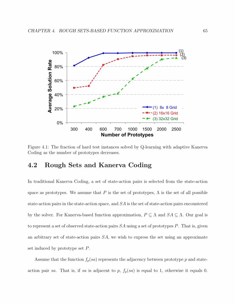
values shown represent the final converged value of the solution rate. The results indicates

that the fraction of test instances solved increased from 73.3% to 96.4% for the 8x8 grid,

from 32.3% to 88.8% for the 16x16 grid, and from 20.8% to 76.4% for the 32x32 grid as the

number of prototypes increases.

By comparing with Table 2.2, we see that adaptive Kanerva Coding achieves a lower

average solution rate when solving hard test instances than when solving easy test instances

when the number of prototypes and the size of the grid are held constant.

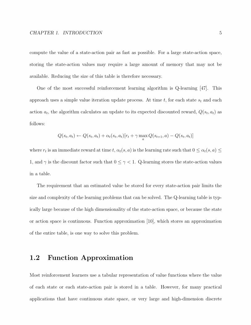
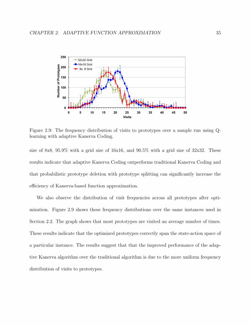
Figure 3.1 shows the average fraction of hard test instances solved by Q-learning with

adaptive Kanerva Coding with 2000 tiles as the size of the grid varies from 8x8 to 32x32. The

graph shows how the solvers converge as the number of epochs increases. The results show

that when using adaptive Kanerva-based function approximation with 2000 prototypes, the

fraction of test instances solved decreases from 94.9% to 67.9% as the grid size increases.

These results indicate that although it improves on traditional Kanerva Coding, the

fraction of test instances solved using adaptive Kanerva Coding still decreases sharply as


0.00

0.10

0.20

0.30

0.40

0.50

0.60

0.70

0.80

0.90

1.00

0 200 400 600 800 1000 1200 1400 1600 1800 2000

Aver

age

solu

tion

rate

Epoch

(1) 8X 8 Grid (2) 16X16 Grid (3) 32X32 Gird

(1)

(2)

(3)

Figure 3.1: The fraction of easy and hard test instances solved by Q-learning with adaptiveKanerva Coding with 2000 prototypes.

the size of the grid increases when applied to hard test instances. Feature optimization only

improves the efficiency of function approximation to a certain extent, and cannot solve hard

instances of large-scale system. We need to further explore other factors that may be causing

poor performance.

3.2 Prototype Collisions in Kanerva Coding

Kanerva Coding is an implementation of SDM for reinforcement learning. A collection of

k prototypes is selected, each of which corresponds to a binary feature. A state-action pair

sa and a prototype pi are adjacent if their bit-wise representations differ by no more than a

threshold number of bits. The threshold is typically set to 1 bit. We define the adjacency

grade adji(sa) of sa with respect to pi to be equal 1 if sa is adjacent to pi, and equal to

0 otherwise. A state-action pair’s prototype vector consists of its adjacency grades with


!"#

!$#

!%#

!&#

sa1

sa2

SA

!"#

!$#

!%#

!&#

sa1

sa2

SA

collision

!"#

!$#

!%#

!&#

sa1 sa

2

SA collision

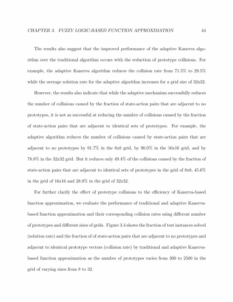
(a) (b) (c)

Figure 3.2: The illustration of prototype collision. (a) adjacent to no prototype; (b) adjacentto an identical prototype set; (c) adjacent to unique prototype vectors.

respect to all prototypes. A value θ(i) is maintained for the ith prototype, and Q(sa), an

approximation of the value of a state-action pair sa, is then the sum of the θ-values of the

adjacent prototypes; that is,

Q(sa) =∑i

θ(i) ∗ adji(sa).

A prototype collision is said to have taken place between two distinct state-action pairs,

sai and saj, if and only if sai and saj have the same prototype vector, that is, the same

adjacency grades over all prototypes.

In Kanerva Coding, for two arbitrary state-action pairs, there are three possible cases: the

state-action pairs are both adjacent to no prototypes, the state-action pairs have identical

prototype vectors, or the state-action pairs have distinct prototype vectors, as shown in

Figure 3.2. Kanerva Coding works best when each state-action pair has a unique prototype

vector, where no prototype collision takes place. If prototypes are not well distributed across


the state-action space, many state-action pairs will either not be adjacent to any prototypes,

or adjacent to identical sets of prototypes, corresponding to identical prototype vectors. If

two similar state-action pairs are adjacent to the same set of prototypes, their state-action

value are always same during the learning process. Typically, the solver needs to distinguish

such state-action pairs, which is not possible in this case. Such prototype collisions reduce

the quality of the results, and the estimates of Q-values of such state-action pairs will be

equal [49]..

The collision rate in Kanerva Coding is the fraction of state-action pairs that are

either adjacent to no prototypes, or adjacent to the same set of prototypes as some other

state-action pair. The larger the value of the collision rate, the more frequently prototype

collisions will occur during Kanerva-based function approximation. The prototype collision

is therefore inversely proportional to the learning performance of a reinforcement learner

with Kanerva-based function approximation.

Selecting a set of prototypes that distinguishes frequently-visit distinct state-actions pairs

can improve the solver’s ability to solve the problem. However, it is difficult to generate such a

set of prototypes for several reasons: the space of possible subsets is very large, and the state-

action pairs encountered by the solver depend on the specific problem instance being solved.

Dynamic prototype allocation and adaptation removes unnecessary prototypes and adds

new prototypes that cover parts of the state-action space that are frequently visited during

instance-based learning. In this way, prototypes can be adaptively adjusted to minimize

prototype collisions for the specific problem domain.


9.4% 0.6%

28.1%

2.8%

43.3%

9.2%

15.6%

7.9%

22.6%

12.3%

28.2%

20.3%

75.0%

91.5%

49.3%

84.9%

28.5%

70.5%

0%

10%

20%

30%

40%

50%

60%

70%

80%

90%

100%

Traditional Adaptive Traditional Adaptive Traditional Adaptive

% o

f Sta

te-a

ctio

n Pa

irs

Grid size

Adjacent to a unique prototype set Adjacent to a non-unique prototype set Adjacent to no prototypes

8X8 16X16 32X32

Figure 3.3: Prototype collisions using traditional and adaptive Kanerva-based function ap-proximation with 2000 prototypes.

In order to evaluate the negative effect of prototype collisions, we observe the collision

rates produced when using traditional Kanerva Coding and adaptive Kanerva Coding as the

size of the grid varies. Figure 3.3 shows the fraction of state-action pairs that are adjacent

to no prototypes, adjacent to identical sets of prototypes, and adjacent to a unique set

of prototypes when traditional Kanerva Coding and adaptive Kanerva Coding with 2000

prototypes are applied to easy predator-prey instances of varying sizes. Here, the collision

rate is the sum of the fraction of state-action pairs that are adjacent to no prototypes and the

fraction of state-action pairs that are adjacent to identical sets of prototypes. These results

show that for the traditional algorithm, the collision rate increases from 25.0% to 71.5% as

the size of grid increases. For the adaptive algorithm space, the collision rate increases from

8.5% to 29.5% as the size of the grid increases.


The results also suggest that the improved performance of the adaptive Kanerva algo-

rithm over the traditional algorithm occurs with the reduction of prototype collisions. For

example, the adaptive Kanerva algorithm reduces the collision rate from 71.5% to 29.5%

while the average solution rate for the adaptive algorithm increases for a grid size of 32x32.

However, the results also indicate that while the adaptive mechanism successfully reduces

the number of collisions caused by the fraction of state-action pairs that are adjacent to no

prototypes, it is not as successful at reducing the number of collisions caused by the fraction

of state-action pairs that are adjacent to identical sets of prototypes. For example, the

adaptive algorithm reduces the number of collisions caused by state-action pairs that are

adjacent to no prototypes by 91.7% in the 8x8 grid, by 90.0% in the 16x16 grid, and by

78.8% in the 32x32 grid. But it reduces only 49.4% of the collisions caused by the fraction of

state-action pairs that are adjacent to identical sets of prototypes in the grid of 8x8, 45.6%

in the grid of 16x16 and 28.0% in the grid of 32x32.

For further clarify the effect of prototype collisions to the efficiency of Kanerva-based

function approximation, we evaluate the performance of traditional and adaptive Kanerva-

based function approximation and their corresponding collision rates using different number

of prototypes and different sizes of grids. Figure 3.4 shows the fraction of test instances solved

(solution rate) and the fraction of of state-action pairs that are adjacent to no prototypes and

adjacent to identical prototype vectors (collision rate) by traditional and adaptive Kanerva-

based function approximation as the number of prototypes varies from 300 to 2500 in the

grid of varying sizes from 8 to 32.


0%

20%

40%

60%

80%

100%

300 600 1000 1500 2000 2500

Sol$on Rate

Number of Prototypes

Tradi0onal

Adap0ve

(a) 8 x 8

0%

20%

40%

60%

80%

100%

300 600 1000 1500 2000 2500

CollisionRate

NumberofPrototypes

Adjacenttouniqueprototypeset

Adjacenttoiden;calprototypeset

Adjacenttonoprototype

3006001000150020002500

Tra.Ada.Tra.Ada.Tra.Ada.Tra.Ada.Tra.Ada.Tra.Ada.

(b) 8 x 8

0%

20%

40%

60%

80%

100%

300 600 1000 1500 2000 2500

Sol$on Rate


Tradi0onal

Adap0ve

(c) 16 x 16

0%

20%

40%

60%

80%

100%

300 600 1000 1500 2000 2500

CollisionRate

NumberofPrototypes




3006001000150020002500


(d) 16 x 16

0%

20%

40%

60%

80%

100%

300 600 1000 1500 2000 2500

Sol$on Rate


Tradi0onal

Adap0ve

(e) 32 x 32

0%

20%

40%

60%

80%

100%

300 600 1000 1500 2000 2500

CollisionRate

NumberofPrototypes




3006001000150020002500


(f) 32 x 32

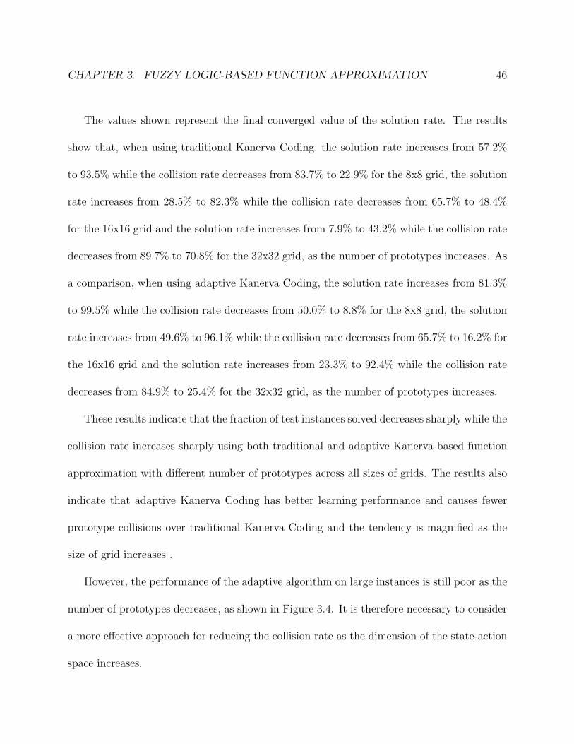
Figure 3.4: Average fraction of test instances solved (solution rate) (a) 8x8 grid; (c) 16x16grid; (e) 32x32 grid, and the fraction of of state-action pairs that are adjacent to no pro-totypes and adjacent to identical prototype vectors (collision rate) (b) 8x8 grid; (d) 16x16grid; (f) 32x32 grid by traditional and adaptive Kanerva-based function approximation asthe number of prototypes varies from 300 to 2500.


The values shown represent the final converged value of the solution rate. The results

show that, when using traditional Kanerva Coding, the solution rate increases from 57.2%

to 93.5% while the collision rate decreases from 83.7% to 22.9% for the 8x8 grid, the solution

rate increases from 28.5% to 82.3% while the collision rate decreases from 65.7% to 48.4%

for the 16x16 grid and the solution rate increases from 7.9% to 43.2% while the collision rate

decreases from 89.7% to 70.8% for the 32x32 grid, as the number of prototypes increases. As

a comparison, when using adaptive Kanerva Coding, the solution rate increases from 81.3%

to 99.5% while the collision rate decreases from 50.0% to 8.8% for the 8x8 grid, the solution

rate increases from 49.6% to 96.1% while the collision rate decreases from 65.7% to 16.2% for

the 16x16 grid and the solution rate increases from 23.3% to 92.4% while the collision rate

decreases from 84.9% to 25.4% for the 32x32 grid, as the number of prototypes increases.

These results indicate that the fraction of test instances solved decreases sharply while the

collision rate increases sharply using both traditional and adaptive Kanerva-based function

approximation with different number of prototypes across all sizes of grids. The results also

indicate that adaptive Kanerva Coding has better learning performance and causes fewer

prototype collisions over traditional Kanerva Coding and the tendency is magnified as the

size of grid increases .

However, the performance of the adaptive algorithm on large instances is still poor as the

number of prototypes decreases, as shown in Figure 3.4. It is therefore necessary to consider

a more effective approach for reducing the collision rate as the dimension of the state-action

space increases.


3.3 Adaptive Fuzzy Kanerva Coding

A more flexible and powerful approach to function approximation is to allow a state-action

pair to update θ-values of all prototypes, instead of a subset of neighbor prototypes. Instead

of being binary values, we use fuzzy membership grades that vary continuously between 0

and 1 across all prototypes. Such fuzzy membership grades are larger for closer prototypes

and smaller for more distant prototypes. Since prototype collisions occur only when two

state-action pairs have the same real values in all elements of their membership vectors,

collisions are less likely.

In the traditional Kanerva Coding, a collection of k prototypes is selected. A state-

action pair sa and a prototype pi are said to be adjacent if their bit-wise representations

differ by no more than a threshold number of bits. To introduce fuzzy membership grades,

we reformulate this definition of traditional Kanerva Coding using fuzzy logic [16, 13, 44].

We define the membership grade µi(sa) of s with respect to pi

µi(sa) =

1 if sa is adjacent to pi,

0 otherwise.

A state-action pair’s membership vector consists of its membership grades with respect to

all prototypes. A value θ(i) is maintained for the ith feature, and Q̂(sa), an approximation of

the value of a state-action pair sa, is then the sum of the θ-values of the adjacent prototypes.

That is

Q̂(sa) =∑i

θ(i)µi(sa).


Figure 3.5: Sample membership function for traditional Kanerva Coding.

Therefore Kanerva Coding can greatly reduce the size of the value table that needs to be

stored.

Figure 3.5 gives an abstract description of the distribution of a state-action pair’s mem-

bership grade with respect to each element of a set of prototypes. The figure shows the

regions of the state-action space where prototype collisions take place. Note that receptive

fields with crisp boundaries can cause frequent collisions.

3.3.1 Fuzzy and Adaptive Mechanism

In our fuzzy approach to Kanerva Coding, the membership grade is defined as follows. Given

a state-action pair s, the ith prototype pi, and a constant variance σ2, the membership grade


Figure 3.6: Sample membership function for fuzzy Kanerva Coding.

of sa with respect to pi is

µi = e−||sa−pi||

2

2σ2 ,

where ||s − pi|| represents the bit difference between sa and pi. Note that the membership

grade of a prototype with respect to an identical state-action pair is 1, and the membership

grade of a state-action pair and a completely different prototype approaches 0.

The effect of an update ∆θ to a prototype’s θ-value is now a continuous function of the

bit difference ||sa−pi|| between the state-action pair s and the prototype pi. The update can

have a large effect on immediately adjacent prototypes, and a smaller effect on more distant

prototypes. Figure 3.6 gives an abstract description of the distribution of a state-action pairs

fuzzy membership grade with respect to each member of a set of prototypes.

In the adaptive Kanerva Coding algorithm described above, prototypes are updated based


on their visit frequencies. In fuzzy Kanerva Coding the visit frequency of each prototype is

identical, so we instead use membership grades which vary continuously from 0 to 1. If the

membership grade of a state-action pair with respect to a prototype tends to 1, we say that

the prototype is strongly adjacent to the state-action pair, Otherwise, the prototype is said

to be weakly adjacent to the state-action pair. The probability pupdate(sa) that a state-action

pair sa is chosen as a prototype is

pupdate(sa) = λe−λm(sa),

where λ is a parameter that can vary from 0 to 1, and where m(sa) is the sum of the

membership grades of state-action pair sa with respect to all prototypes. In this mecha-

nism, prototypes that are weakly adjacent to frequently-visited state-action pairs tend to

be probabilistically replaced by prootypes that are strongly adjacent to frequently-visited

state-action pairs.

3.3.2 Adaptive Fuzzy Kanerva Coding Algorithm

Algorithm 1 describes our adaptive fuzzy Kanerva Coding algorithm. The algorithm begins

by initializing parameters and repeatedly executes Q-learning with fuzzy Kanerva Coding.

Prototypes are adaptively updated periodically. The algorithm computes fuzzy membership

grades for all state-action pairs with respect to all prototypes. Current prototypes are then

periodically probabilistically replaced with state-action pairs with the highest accumulated

membership grades.


Algorithm 1 Pseudo Code of Fuzzy Kanerva Coding

Main()

choose a set of prototypes ~p and initial their ~θ value;repeat

Generate initial state-action pair s from initial state ς and action aQ-with-Kanerva(s, a, ~p, ~θ)

Update-prototypes(~p, ~θ)until all episodes are traversed

Q-with-Kanerva(s, a, ~p, ~θ)repeat

Take action a, observe reward r, get next state ς’

~µ(s) = e

„− ||s−~p||

2

2σ2

«;

Q̂(s) =∑~µ(s) ∗ ~θ;

for all actions a* under new state ς’ doGenerate the state-action pair s’ f̄rom state ς’ and action a*;

~µ(s′) = e

„− ||s

′−~p||2

2σ2

«;

Q̂(s) =∑~µ(s′) ∗ ~θ;

end forδ = r + γ ∗maxQ(s′)−Q(s);

∆~θ = α ∗ δ ∗ ~µ(s);~θ = ~θ + ∆~θ;m(s) = m(s) + ~µ(s);if random probability ≤ ε then

for all actions a* under current state s doQ̂(s) =

∑~µ(s) ∗ ~θ;

a = argmaxaQ(sa)end for

elsea = random action

end ifuntil s is terminal

Update-prototypes(~p, ~θ)~p = φrepeat

for all state-action pairs s dowith probability λe−λm(s)

~p = ~p⋃{s}

end foruntil ~p is full


Table 3.2: The average fraction of test instances solved by Q-Learning with adaptive fuzzyKanerva Coding.

# of Prot. 8x8 16x16 32x32

300 80.9% 42.8% 20.9%400 84.5% 50.0% 25.5%600 91.0% 61.8% 39.0%700 91.1% 67.2% 41.2%1000 93.0% 71.2% 58.6%1500 95.4% 86.7% 78.4%2000 97.3% 91.6% 82.8%2500 97.5% 92.2% 85.3%

3.3.3 Performance Evaluation of Adaptive Fuzzy Kanerva-Based

Function Approximation

We evaluate the performance of adaptive fuzzy Kanerva Coding by applying Q-learning

with adaptive Kanerva Coding and adaptive fuzzy Kanerva Coding with different number

of prototypes to hard pursuit instances on grids of various sizes.

Table 3.2 shows the average fraction of hard test instances solved by Q-learning with

fuzzy Kanerva Coding as the number of prototypes and the size of the grid vary. The values

shown represent the final converged value of the solution rate. The results indicates that the

fraction of test instances solved increased from 80.9% to 97.5% for the 8x8 grid, from 42.8%

to 92.2% for the 16x16 grid, and from 20.9% to 85.3% for the 32x32 grid as the number of

prototypes increases.

By comparing with Table 3.1, we see that the fuzzy Kanerva Coding increases the average

solution rate over the adaptive Kanerva Coding when the number of prototypes and the size

of the grid are held constant.


!"##$%!"##$%

!"##$%

&'()$%

&'()$%

&'()$%

*%

*$+%

*$,%

*$-%

*$.%

*$/%

*$0%

*$1%

*$2%

*$3%

+%

+% ,% -%

!"#$%&#'()*+,

)-'.%/#'

0$12'(13#'

242% +04+0% -,4-,%

0.00

0.10

0.20

0.30

0.40

0.50

0.60

0.70

0.80

0.90

1.00

0 200 400 600 800 1000 1200 1400 1600 1800 2000

Avera

ge s

olu

tio

n r

ate

Epoch

(1) 8X 8 Grid, Fuzzy

(2) 8X 8 Grid, Adaptive

(3) 16X16 Grid, Fuzzy

(4) 16X16 Grid, Adaptive

(5) 32X32 Grid, Fuzzy

(6) 32X32 Grid, Adaptive,

!"#$!%#$

!&#$!'#$

!(#$

!)#$

Figure 3.7: Average solution rate for adaptive fuzzy Kanerva Coding with 2000 prototypes.

Figure 3.7 shows the average fraction of test instances solved when adaptive Kanerva and

adaptive fuzzy Kanerva-based function approximation are applied to our instances as the

number of prototypes varies. The results show that with 2000 prototypes, using the fuzzy

algorithm increases the fraction of the test instances solved over the adaptive algorithm from

83.4% to 91.6% in the grid of 16x16 and from 67.9% to 82.8% in the grid of 32x32. These

results indicates that the fuzzy algorithm increases the fraction of the test instances solved

over the adaptive Kanerva algorithm.


3.4 Prototype Tuning

While fuzzy Kanerva Coding can give good results for our instances, the quality of the results

is often unstable. That is, the average fraction of test instances solved by the fuzzy approach

may be low. An explanation for these results can be found by considering the similarity

of membership vectors across state-action pairs. Intuitively, the similarity of membership

vectors of state-action pairs is equivalent to the prototype collisions observed with traditional

Kanerva Coding. In both cases, it may reduce the quality of the results.

3.4.1 Experimental Evaluation: Similarity Analysis of Member-

ship Vectors

Figure 3.8(a) shows the average membership grade of each prototype with respect to all other

prototypes on a sample run. The prototypes are ordered by decreasing average membership

grade. The results show that prototypes fall into three general regions. On the left, the pro-

totypes have a higher average membership grade, corresponding to prototypes that are closer

on average to other prototypes. On the right, prototypes have a lower average membership

grade, corresponding to prototypes that are on average farther from other prototypes. The

prototypes on the left are in a region of the state-action space where the distribution of

prototypes is more dense, and prototypes on the right are in a region where the distribution

of prototypes is more sparse. This variation in the distribution of the prototypes causes the

receptive fields to be unevenly distributed across the state-action space.

State-action pairs in the dense region of the space are near to more prototypes and


Figure 3.8: (a) Distribution of membership grades and (b) prototype similarity across sortedprototypes.

therefore have large membership grades that are near the top of the Gaussian response

function. Similarly, state-action pairs in the sparse region of the space are far from more

prototypes and therefore have small membership grades that are near the tail of the Gaussian

response function. A state-action pair’s membership grade is less sensitive to variations when

the membership grade is near 1 or 0, as illustrated in Figure 3.9(a). Two state-action pairs in

the dense region are therefore more likely to have membership vectors that are similar, and

the same is true for two state-action pairs in the sparse region. This similarity between the

membership vectors of state-action pairs is equivalent to the prototype collisions observed


A prototype’s membership

function

(a) Before prototype tuning.

A prototype’s

membership function

(b) After prototype tuning.

Figure 3.9: Illustration of the similarity of membership vectors across sparse and denseprototype regions.

with traditional Kanerva Coding, and may have a similar negative effect on the quality of

the results.

Figure 3.9(b) illustrates how the similarity between prototypes can vary across the state-

action space. The graph shows the average Euclidean distance between each prototype and

every other prototype. Prototypes in the dense and sparse regions have a smaller average

Euclidean distance, indicating that they are more similar to one another.


3.4.2 Tuning Mechanism

We can reduce the effect of similar membership vectors by adjusting the variance of the

Gaussian response function used to compute membership grades. The variance is decreased

in the dense region which narrows the Gaussian response function, and the variance is in-

creased in the sparse region which broadens the Gaussian response function. This prototype

tuning increases the sensitivity of state-action pairs’ membership vectors to variations in the

state-action space in these regions, as shown in Figure 3.9(b). We use Maximum Likelihood

Estimation to compute an estimate σ̂2i of the variance of a prototype’s membership func-

tion. Given a prototype i, we let dij be the bit difference between prototype pi and all other

prototypes pj, where j 6= i, and d̄i the sample mean of dij. The estimate of σ̂2i is

σ̂2i =

n∑j=1

(dij − d̄i)2/n,

where n is the number of prototypes.

3.4.3 Performance Evaluation of Tuning Mechanism

We evaluate our implementation of adaptive fuzzy Kanerva Coding with prototype tuning

by using it to solve pursuit instances on a grid of size 32x32. As a comparison, the adaptive

fuzzy and adaptive approaches are also implemented to solve the same instances.

Figure 3.10 shows the average fraction of test instances solved by adaptive fuzzy Kanerva

Coding with prototype tuning. We can see that using prototype tuning increases the fraction

of the test instances solved over the adaptive fuzzy algorithm and the adaptive algorithm.

For example, with 2000 prototypes, using prototype tuning increases the fraction of the test


0.00 0.10 0.20 0.30 0.40 0.50 0.60 0.70 0.80 0.90 1.00

0 200 400 600 800 1000 1200 1400 1600 1800 2000

Aver

age

solu

tion

rate

Epoch

(1) Fuzzy Kanerva with Tuning (2) Fuzzy Kanerva (3) Adaptive Kanerva

(1)

(2)

(3)

Figure 3.10: Average solution rate for adaptive fuzzy Kanerva Coding with Tuning using2000 prototypes.

instances solved over the adaptive and fuzzy algorithm from 67.9% and 82.8% to 97.1%.

These results demonstrate that using prototype tuning can greatly improve the efficiency of

adaptive fuzzy Kanerva Coding.

We further evaluate our adaptive fuzzy Kanerva Coding algorithm with prototype tuning

by applying it to solve the four-room problem employed by Sutton, Precup and Singh [41]

and Stone and Veloso [37]. To increase the size of the state space, we extend the grid to size

32x32, shown in Figure 3.11. Pursuit takes place on a rectangular grid with 4 rooms. The

agent can move to a neighboring open cell one horizontal or vertical step from its current

location, or it can remain in its current cell. To go to another room, the agent must pass

through a door. The agent is randomly placed in a starting cell, and the agent attempts to

reach a fixed goal cell. The agent receives a reward of 1 when it reaches the goal cell, and


Figure 3.11: The four-room gridworld

receives a reward of 0 in every other cell.

Figure 3.12 compares the average fraction of test instances solved by adaptive fuzzy

Kanerva Coding with prototype tuning to solve the instances of the four-room problem. The

results show that using adaptive fuzzy Kanerva Coding with prototype tuning increases the

fraction of the test instances solved over using adaptive and adaptive fuzzy approaches. For

example, using adaptive fuzzy Kanerva Coding with prototype tuning with 2000 prototypes

increases the fraction of the test instances solved over using adaptive and adaptive fuzzy

approaches from 58.4% and 78.9% to 94.9%. These results again demonstrate that using

adaptive fuzzy Kanerva Coding with prototype tuning can greatly improve the quality of


0.00 0.10 0.20 0.30 0.40 0.50 0.60 0.70 0.80 0.90 1.00

0 200 400 600 800 1000 1200 1400 1600 1800 2000

Aver

age

solu

tion

rate

Epoch

(1) Fuzzy Kanerva with Tuning (2) Fuzzy Kanerva (3) Adaptive Kanerva

(1)

(2)

(3)

Figure 3.12: Average solution rate for adaptive Fuzzy Kanerva Coding with Tuning in thefour-room gridworld of size 32x32.

the results obtained.

3.5 Summary

In this chapter, we evaluated a class of hard pursuit instances of the predator-prey prob-

lem and argued that this poor performance is caused by frequent prototype collisions. We

also showed that dynamic prototype allocation and adaptation can partially reduce these

collisions and give better results. However the collision rate remained quite high and the

performance was still poor for large-scale instances. It was therefore necessary to consider a

more effective approach for eliminating the collision rate as the dimension of the state-action

space increases.

Our new fuzzy approach to Kanerva-based function approximation uses a fine-grained


fuzzy membership grade to describe a state-action pair’s adjacency with respect to each

prototype. This approach, coupled with adaptive prototype allocation, allows the solver to

distinguish membership vectors and reduce the collision rate. Our adaptive fuzzy Kanerva

approach gives better performance than the pure adaptive Kanerva algorithm. We then

showed that prototype density varies widely across the state-action space, causing prototypes’

receptive fields to be unevenly distributed across the state-action space. State-action pairs

in dense or sparse regions of the space are more likely to have similar membership vectors

which limits the performance of a reinforcement learner based on Kanerva Coding. Our

fuzzy framework for Kanerva-based function approximation allows us to tune the prototype

receptive fields to balance the effects of prototype density variations, further increasing the

fraction of test instances solved using this approach. We conclude that adaptive fuzzy

Kanerva Coding with prototype tuning can significantly improve a reinforcement learner’s

ability to solve large-scale high dimension problems.

Chapter 4

Rough Sets-based Function

Approximation

Fuzzy Kanerva-based function approximation can significantly improve the efficiency of

function approximation within reinforcement learners. As we described in Chapter 3, this

approach distinguishes frequently-visited state-actions pairs by using a fine-grained fuzzy

membership grade to describe a state-action pair’s adjacency with respect to each proto-

type. In this way, the fuzzy approach completely eliminates prototype collisions. We have

shown that this approach gives a function approximation architecture that outperforms other

approaches.

However, our experimental results show that this approach often gives poor performance

when solving hard large-scale instances and shows unstable behavior when changing the

62

CHAPTER 4. ROUGH SETS-BASED FUNCTION APPROXIMATION 63

number of prototypes. We therefore extend our work to improve our algorithm. In this

chapter, we show that choosing an optimal number of prototypes can improve the efficiency

of function approximation. We propose to use the theory of rough sets to measure how

closely an approximate value function is approximating the true value function and determine

whether more prototypes are required. Finally, we describe a rough sets-based approach to

selecting prototypes for a Kanerva-based reinforcement learner.

4.1 Experimental Evaluation: Effect of Varying Num-

ber of Prototypes

The efficiency of Kanerva-based function approximation depends largely on the number

of prototypes. It is clear that the efficiency of our function approximator decreases as the

number of prototypes decreases. We therefore investigate the performance of a reinforcement

learner with adaptive Kanerva Coding as the number of prototypes decreases.

We evaluate the effect of varying the number of prototypes by applying Q-learning with

adaptive Kanerva Coding to the class of predator-prey pursuit instances. The state-action

pairs are represented as prototype vectors and all prototypes are selected randomly. Prob-

abilistic prototype deletion with prototype splitting is used as feature optimization. The

number of prototypes varies from 300 to 2500. The size of the grid varies from 8x8 to 32x32.

Table 4.2 shows the average fraction of test instances solved by Q-learning with adaptive

Kanerva Coding as the number of prototypes and the size of the grid vary. The values shown


Table 4.1: The average fraction of test instances solved by Q-Learning with adaptive KanervaCoding.

Prototypes 8x8 16x16 32x32

300 81.3% 49.6% 23.3%400 92.3% 52.3% 28.3%600 98.9% 82.4% 37.0%700 99.0% 90.4% 41.7%1000 99.2% 94.5% 62.8%1500 99.3% 95.7% 77.6%2000 99.5% 95.9% 90.5%2500 99.5% 96.1% 92.4%

represent the final converged value of the solution rate. The results show that the average

fraction of test instances solved by adaptive Kanerva Coding decreases as the number of

prototypes decreases, which is similar with the behaviors under both traditional and adaptive

fuzzy Kanerva Coding.

Figure 4.1 shows the average fraction of hard test instances solved by Q-learning with

adaptive Kanerva Coding as the number of prototypes decreases from 2500 to 300. The

results show that when the number of prototypes decreases, the fraction of test instances

solved decreases from 99.5% to 81.3% in the 8x8 grid, from 96.1% to 49.6% in the 16x16 grid,

and from 92.4% to 23.3% in the 32x32 grid. This indicates that the efficiency of adaptive

Kanerva-based function approximation does increase as the number of prototypes increases.

Unfortunately, we often do not have enough memory to store a large number of proto-

types. We must therefore consider how to generate an appropriate number of prototypes

that can improve the efficiency of Kanerva-based function approximation.


0%

20%

40%

60%

80%

100%

300 400 600 700 1000 1500 2000 2500

Aver

age

Solu

tion

Rat

e


(1) 8x 8 Grid (2) 16x16 Grid (3) 32x32 Grid

(1)(2)(3)

Figure 4.1: The fraction of hard test instances solved by Q-learning with adaptive KanervaCoding as the number of prototypes decreases.

4.2 Rough Sets and Kanerva Coding

In traditional Kanerva Coding, a set of state-action pairs is selected from the state-action

space as prototypes. We assume that P is the set of prototypes, Λ is the set of all possible

state-action pairs in the state-action space, and SA is the set of state-action pairs encountered

by the solver. For Kanerva-based function approximation, P ⊆ Λ and SA ⊆ Λ. Our goal is

to represent a set of observed state-action pairs SA using a set of prototypes P . That is, given

an arbitrary set of state-action pairs SA, we wish to express the set using an approximate

set induced by prototype set P .

Assume that the function fp(sa) represents the adjacency between prototype p and state-

action pair sa. That is, if sa is adjacent to p, fp(sa) is equal to 1, otherwise it equals 0.


Table 4.2: Sample of adjacency between state-action pairs and prototypes.p1 p2 p3 p4 p5 p6

sa1 0 0 0 0 1 1sa2 1 0 0 1 1 1sa3 1 1 0 0 0 1sa4 0 1 0 0 1 1sa5 0 1 0 0 1 1sa6 1 1 0 1 0 1sa7 0 0 0 0 0 1sa8 0 0 0 0 0 1sa9 0 1 1 1 1 1sa10 0 0 0 0 0 1

The set of adjacency values for a state-action pair with respect to all prototypes is referred

as the state-action pair’s prototype vector. On the basis of prototype set P , we define an

indiscernibility relation, denoted IND(P ):

IND(P ) = {(sa1, sa2) ∈ Λ2|∀p ∈ P, fp(sa1) = fp(sa2)}.

where p is a prototype and sa1 and sa2 are two state-action pairs, that is, sa1 ∈ SA,

sa2 ∈ SA. If any two state-action pairs sa1 and sa2 in the set SA are indiscernible by the

prototypes in P , there is an associated indiscernibility relation between sa1 and sa2. The

set of state-action pairs with the same indiscernibility relation is defined as an equivalence

class, and the ith such equivalence class is denoted EPi . The set of prototypes P therefore

partitions the set SA into a collection of equivalence classes, denoted {EP}.

For example, assume ten state-action pairs, (sa1, sa2, sa3, ..., sa10), are encountered

by a solver, and we have six prototypes, (p1, p2, p3, ..., p6). We attempt to express each

state-action pair using prototypes. Table 4.2 shows a sample of the adjacencies between

state-action pairs and prototypes. When the prototypes are considered, we can induce the


ΛSA

sa1 sa2 sa3

sa4

sa5 sa6

sa9

sa7

sa8 sa10

EP1

EP2

EP3

EP4

EP5 EP

6 EP7

Figure 4.2: Illustration of equivalence classes of the sample.

following equivalence classes, (EP1, E

P2, E

P3, E

P4, E

P5, E

P6, E

P7, ) = ({sa1}, {sa2}, {sa3},

{sa4, sa5}, {sa9}, {sa6}, {sa7, sa8, sa10}). Figure 4.2 shows an illustration of the equivalence

classes of the sample.

The structure of equivalence classes induced by the prototype set has a significant effect

on function approximation. Kanerva Coding works best when each state-action pair has a

unique prototype vector. That is, the ideal set of equivalence classes induced by the prototype

set should each include no more than one state-action pair. If two or more state-action pairs

are in the same equivalence class, these state-action pairs are indiscernible with respect to

the prototypes, causing a prototype collision. The definition of prototype collision can be

found in Section 3.2.


Given a set of prototypes, one or more prototypes may not affect the structure of the

induced equivalence classes, and therefore do not help differentiate state-action pairs. These

prototypes can be replaced with prototypes that are more useful. To do this, we use a

reduct of the prototype set. A reduct is a subset of prototypes R ⊆ P such that (1)

{ER} = {EP}, that is, the equivalence classes induced by reduced prototype set R are the

same as the equivalence classes induced by original prototype set P; and (2) R is minimal,

that is {E(R−{p})} 6= {EP} for any prototype p ∈ R. Thus, no prototype can be removed

from reduced prototype set R without changing the equivalence classes EP .

In the above example, the subset (p2, p4, p5) is a reduct of the original prototype set

P . This can be shown easily because (1) the equivalence classes induced by (p2, p4, p5) are

the same as the equivalence class structure induced by the original prototype set P; and (2)

eliminating any of these prototypes alters the equivalence class structure that is induced.

Replacing a set of prototypes with its reduct eliminates unnecessary prototypes. Adaptive

prototype optimization can also eliminate unnecessary prototypes by deleting rarely-visited

prototypes, but that approach cannot eliminate prototypes that are heavily-visited but un-

necessary, such as prototype p6 in the above example. Note that all state-action pairs are

adjacent to this prototype, but deleting it does not change the structure of the equivalence

classes.

We evaluate the structure of equivalence classes and the reduct of prototypes in traditional

Kanerva Coding and adaptive Kanerva Coding. We apply traditional Kanerva and adaptive

Kanerva with 2000 prototypes to sample predator-prey instances of varying sizes.


93.1%

25.0% 27.6%0%

20%

40%

60%

80%

100%

Solution Rate Collision Rate Conflict Rate

Percentage

8 x 8 Grid, Traditional Kanerva

75.4%50.7% 47.6%

0%

20%

40%

60%

80%

100%

Solution Rate Collision Rate Conflict Rate Percentage


40.6%

71.5% 79.5%

0%

20%

40%

60%

80%

100%


Percentage


99.5%

8.5% 8.2%0%

20%

40%

60%

80%

100%


Percentage

8 x 8 Grid, Adaptive Kanerva

95.9%

15.1% 16.5%0%

20%

40%

60%

80%

100%


Percentage


90.5%

29.5% 35.2%

0%

20%

40%

60%

80%

100%


Percentage


Figure 4.3: The fraction of equivalence classes that contain two or more state-action pairsover all equivalence classes, the conflict rate, and its corresponding solution rate and colli-sion rate using traditional Kanerva and adaptive Kanerva with frequency-based prototypeoptimization across all sizes of grids

Figure 4.3 shows the fraction of equivalence classes that contain two or more state-

action pairs over all equivalence classes, the conflict rate, and its corresponding solution rate

and collision rate using traditional Kanerva and adaptive Kanerva with frequency-based

prototype optimization across all sizes of grids. These results show that as the fraction of

equivalence classes that contain two or more state-action pairs increases, the collision rate

increases and the performance of each algorithm decreases. For example, for the traditional

algorithm, the collision rate increases from 25.0% to 71.5% and the average solution rate

decreases from 93.1% to 40.6%, while the fraction of equivalence classes that contain two

or more state-action pairs increases from 27.6% to 79.5% as the size of the grid increases.


For the adaptive algorithm, the collision rate increases from 8.5% to 29.5% and the average

solution rate decreases from 99.5% to 90.5%, while the fraction of equivalence classes that

contain two or more state-action pairs increases from 8.2% to 35.2% as the size of the grid

increases.

The results also demonstrate that the improved performance of the adaptive Kanerva

algorithm over the traditional algorithm is due to the reduction of the fraction of equivalence

classes that contain two or more state-action pairs. For example, the adaptive algorithm

reduces the fraction of equivalence classes that contain two or more state-action pairs from

79.5% to 35.2% while the average solution rate for the adaptive algorithm increases from

40.6% to 90.5% for a grid size of 32x32.

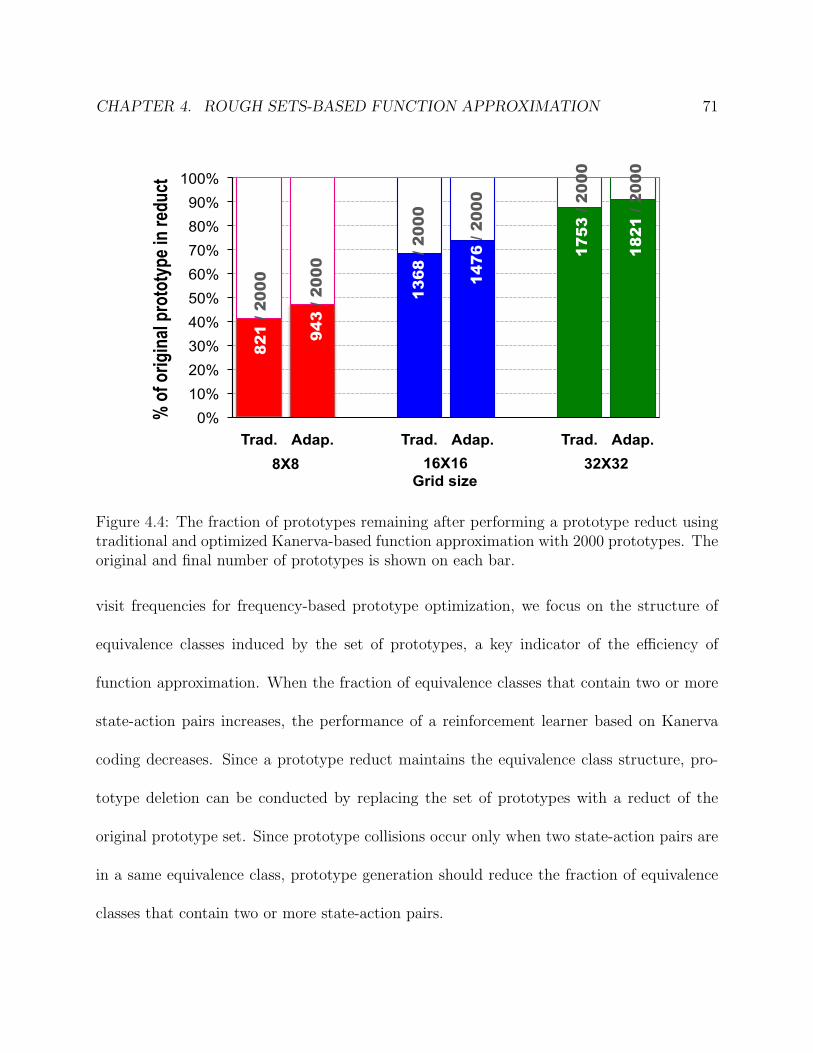
Figure 4.4 shows the fraction of prototypes remaining after performing a prototype reduct

using traditional and optimized Kanerva-based function approximation with 2000 proto-

types. The original and final number of prototypes is shown on each bar. The results

indicate that the structure of the equivalence classes can be maintained using fewer proto-

types. For example, the equivalence classes induced by 1821 prototypes for the adaptive

algorithm using frequency-based prototype optimization are same as the equivalence classes

induced by 2000 prototypes for a grid size of 32.

4.3 Rough Sets-based Kanerva Coding

A more reliable approach to prototype optimization for function approximation is to apply

rough sets theory to reformulate Kanerva-based function approximation. Instead of using


0% 10% 20% 30% 40% 50% 60% 70% 80% 90%

100%

Trad. Adap. Trad. Adap. Trad. Adap.

% of

origi

nal p

roto

type i

n red

uct

Grid size 8X8 16X16 32X32

821

/ 200

0

943

/ 200

0

1368

/ 20

00

1476

/ 20

00

1753

/ 20

00

1821

/ 20

00

Figure 4.4: The fraction of prototypes remaining after performing a prototype reduct usingtraditional and optimized Kanerva-based function approximation with 2000 prototypes. Theoriginal and final number of prototypes is shown on each bar.

visit frequencies for frequency-based prototype optimization, we focus on the structure of

equivalence classes induced by the set of prototypes, a key indicator of the efficiency of

function approximation. When the fraction of equivalence classes that contain two or more

state-action pairs increases, the performance of a reinforcement learner based on Kanerva

coding decreases. Since a prototype reduct maintains the equivalence class structure, pro-

totype deletion can be conducted by replacing the set of prototypes with a reduct of the

original prototype set. Since prototype collisions occur only when two state-action pairs are

in a same equivalence class, prototype generation should reduce the fraction of equivalence

classes that contain two or more state-action pairs.


4.3.1 Prototype Deletion and Generation

In rough sets-based Kanerva coding, if the structure of equivalence classes remains un-

changed, the efficiency of function approximation is also unchanged. Replacing a set of

prototypes with its reduct clearly eliminates unnecessary prototypes. We therefore imple-

ment prototype deletion by finding a reduct R of original prototype set P . We refer to this

approach as reduct-based prototype deletion.

Note that a reduct of prototype set is not necessarily unique, and there may be many

subsets of prototypes which preserve the equivalence-class structure. The following algorithm

finds a reduct of original prototype set. We consider each prototype in P one by one. For

prototype p ∈ P , if the set of equivalence classes {EP−{p}} induced by P − {p} is not identical

to the equivalence classes {EP} induced by P , that is, {EP−{p}} 6= {EP}, then p is in a reduct

R of original prototype set P , p ∈ R; otherwise, p is not in the reduct R, p /∈ R. We then

delete p from prototype set P and consider the next prototype. The final set R is a reduct

of original prototype set P . We find a series of random reducts of the original prototype set,

then select a reduct with the fewest elements to be the replacement of original prototype

set. Reduct-based prototype optimization makes only a few passes through the prototypes

and is not time-consuming. With n state-action pairs and p prototypes, the complexity is

O(n ∗ p2). Once a prototype is deleted, the θ-value of this prototype is accumulated to the

nearest prototypes.

In rough sets-based Kanerva coding, if the number of equivalence classes that contain

only one state-action pair increases, prototype collisions are less likely and the efficiency of


function approximation increases. An equivalence class that contains two or more state-

action pairs is likely to be split up by adding a new prototype equal to one of those state-

action pairs. We therefore implement prototype generation by adding new prototypes that

split equivalence classes with two or more state-action pairs. We refer to this approach as

equivalence class-based prototype generation.

For an arbitrary equivalence class that contains n > 1 state-ation pairs, we randomly

select dlog(n)e state-ation pairs to be new prototypes. Note that this value is the smallest

number of prototypes needed to distinguish all state-action pairs in an equivalence class that

contains n elements. This algorithm does not guarantee that each equivalence class will be

split into new classes that contain exactly one state-action pair. For example, this approach

cannot split an equivalence class with two neighboring state-action pairs. In this case, we

add such a new prototype that is a neighbor of one state-action pair, but not a neighbor of

the other.

4.3.2 Rough Sets-based Kanerva Coding Algorithm

Algorithm 2 describes our algorithm for implementing Q-learning with adaptive Kanerva

coding using rough sets-based prototype optimization. The algorithm begins by initializing

parameters, and repeatedly executes Q-learning with adaptive Kanerva Coding. Prototypes

are adaptively updated periodically. In each update period, the encountered state-action

pairs are recorded. To update prototypes, the algorithm first determines the structure of

the equivalence classes of the set of encountered state-action pairs with respect to original


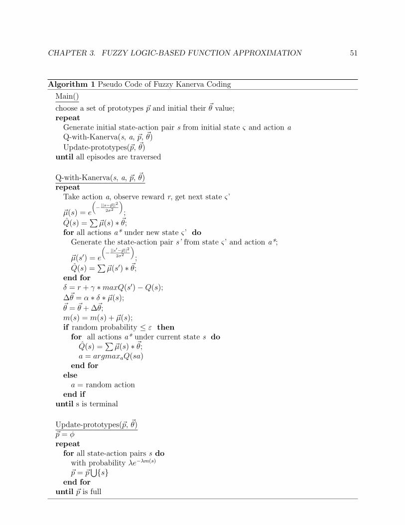
Algorithm 2 Pseudo code of Q-learning with rough sets-based Kanerva Coding

Main()

choose a set of prototypes ~p and initial their ~θ value;repeat

Generate initial state-action pair s from initial state ς and action aQ-with-Kanerva(s, a, ~p, ~θ)

Update-prototypes(~p, ~θ)until all episodes are traversed

Q-with-Kanerva(s, a, ~p, ~θ)repeat

Take action a, observe reward r, get next state ς’Q(sa) =

∑ ~θ;for all actions a* under new state ς’ do

Generate the state-action pair sa’ from state ς’ and action a*Q(sa′) =

∑ ~θ;end forδ = r + γ ∗maxQ(s′)−Q(sa)

∆~θ = α ∗ δ~θ = ~θ + ∆~θif random probability ≤ ε then

for all actions a* under current state s doQ̂(sa) =

∑ ~θ;a = argmaxaQ(sa)

end forelsea = random action

end ifuntil s is terminal

Update-prototypes(~p, ~θ)

Prototype-reduct-based-Deletion(~p, ~θ);

Equivalent-class-based-Generation(~p, ~θ).


Prototype-reduct-based-Deletion(~p, ~θ)−−→E(~p) = equivalence classes induced by ~p~preduct = ~pfor i = 0 to 10 do~ptmp = ~prepeat~̂p = ~ptmp − p−−→E(~̂p) = equivalence classes induced by ~̂p

if−−→E(~̂p) =

−−→E(~p) then

~ptmp = ~̂pend if

until all prototypes p ∈ ~ptmp are traversed.if |~preduct| > |~ptmp| then~preduct = ~ptmp

end ifend for

Equivalent-class-based-Generation(~p, ~θ)repeatn = size(E(~p))if n > 1 then

if (n = 2) and (two state-action pairs sa1 and sa2 are neighbor) then~p = ~p

⋃{p|p = a neighbor of sa1, but not a neighbor of sa2}

elserepeat

randomly select a state-action pair sa~p = ~p

⋃{sa}

until dlog(n)e new prototypes are generated.end if

end if

until all equivalence classes E(~p) ∈−−→E(~p) are traversed.


prototypes. Unnecessary prototypes are then deleted by replacing the original prototype set

with a reduct with the fewest elements among ten randomly-generated reducts. In order to

split large equivalence classes, new prototypes are randomly selected from these equivalence

classes. For the equivalence classes with two neighboring state-action pairs, a new prototype

is a neighbor of one state-action pair, but not a neighbor of the other. The optimized

prototype set is constructed by adding newly generated prototypes to the reduct of original

prototype set.

4.3.3 Performance Evaluation of Rough Sets-based Kanerva Cod-

ing

We evaluate the performance of rough sets-based Kanerva coding by using it to solve pursuit

instances on grids of varying sizes. As a comparison, traditional Kanerva coding and adaptive

Kanerva coding with different number of prototypes are also applied to the same instances.

Traditional Kanerva coding follows Sutton [38]. Kanerva coding with adaptive prototype

optimization is implemented using prototype deletion and prototype splitting. A detailed

description of prototype deletion and splitting can be found in Section 3.3. When rough

sets-based Kanerva coding is implemented during a learning process, we also observe the

change in the number of prototypes and the fraction of equivalence classes that contain only

one state-action pair.

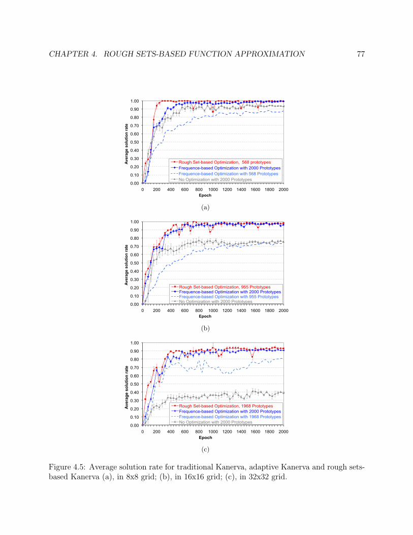
Figure 4.5 shows the average fraction of test instances solved when traditional Kanerva,

adaptive Kanerva, and rough sets-based Kanerva are applied to our instances with grids of


0.00

0.10

0.20

0.30

0.40

0.50

0.60

0.70

0.80

0.90

1.00

0 200 400 600 800 1000 1200 1400 1600 1800 2000

Aver

age

solu

tion

rate

Epoch

Rough Set-based Optimization, 568 prototypes Frequence-based Optimization with 2000 Prototypes Frequence-based Optimization with 568 Prototypes No Optimization with 2000 Prototypes

(a)

0.00

0.10

0.20

0.30

0.40

0.50

0.60

0.70

0.80

0.90

1.00

0 200 400 600 800 1000 1200 1400 1600 1800 2000

Aver

age

solu

tion

rate

Epoch

Rough Set-based Optimization, 955 Prototypes Frequence-based Optimization with 2000 Prototypes Frequence-based Optimization with 955 Prototypes No Optimization with 2000 Prototypes

(b)

0.00

0.10

0.20

0.30

0.40

0.50

0.60

0.70

0.80

0.90

1.00

0 200 400 600 800 1000 1200 1400 1600 1800 2000

Aver

age

solu

tion

rate

Epoch

Rough Set-based Optimization, 1968 Prototypes Frequence-based Optimization with 2000 Prototypes Frequence-based Optimization with 1968 Prototypes No Optimization with 2000 Prototypes

(c)

Figure 4.5: Average solution rate for traditional Kanerva, adaptive Kanerva and rough sets-based Kanerva (a), in 8x8 grid; (b), in 16x16 grid; (c), in 32x32 grid.


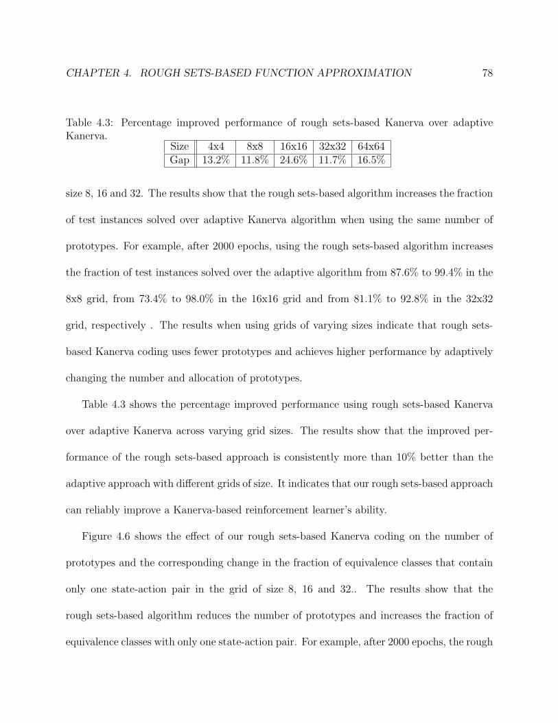
Table 4.3: Percentage improved performance of rough sets-based Kanerva over adaptiveKanerva.

Size 4x4 8x8 16x16 32x32 64x64Gap 13.2% 11.8% 24.6% 11.7% 16.5%

size 8, 16 and 32. The results show that the rough sets-based algorithm increases the fraction

of test instances solved over adaptive Kanerva algorithm when using the same number of

prototypes. For example, after 2000 epochs, using the rough sets-based algorithm increases

the fraction of test instances solved over the adaptive algorithm from 87.6% to 99.4% in the

8x8 grid, from 73.4% to 98.0% in the 16x16 grid and from 81.1% to 92.8% in the 32x32

grid, respectively . The results when using grids of varying sizes indicate that rough sets-

based Kanerva coding uses fewer prototypes and achieves higher performance by adaptively

changing the number and allocation of prototypes.

Table 4.3 shows the percentage improved performance using rough sets-based Kanerva

over adaptive Kanerva across varying grid sizes. The results show that the improved per-

formance of the rough sets-based approach is consistently more than 10% better than the

adaptive approach with different grids of size. It indicates that our rough sets-based approach

can reliably improve a Kanerva-based reinforcement learner’s ability.

Figure 4.6 shows the effect of our rough sets-based Kanerva coding on the number of

prototypes and the corresponding change in the fraction of equivalence classes that contain

only one state-action pair in the grid of size 8, 16 and 32.. The results show that the

rough sets-based algorithm reduces the number of prototypes and increases the fraction of

equivalence classes with only one state-action pair. For example, after 2000 epochs, the rough


2000 Prototypes

568 Prototypes

0%

10%

20%

30%

40%

50%

60%

70%

80%

90%

100%

0

500

1000

1500

2000

2500

0 200 400 600 800 1000 1200 1400 1600 1800 2000

% o

f equ

ival

ence

cla

sses

that

con

tain

onl

y on

e st

ate-

actio

n pa

ir

Num

ber o

f pro

toty

pes

Epoch

(a)

2000 Prototypes

955 Prototypes

0%

10%

20%

30%

40%

50%

60%

70%

80%

90%

100%

0

500

1000

1500

2000

2500

0 200 400 600 800 1000 1200 1400 1600 1800 2000

% o

f equ

ival

ence

cla

sses

that

con

tain

onl

y on

e st

ate-

actio

n pa

ir

Num

ber o

f pro

toty

pes

Epoch

(b)

2000 Prototypes 1968 Prototypes

0%

10%

20%

30%

40%

50%

60%

70%

80%

90%

100%

0

500

1000

1500

2000

2500

0 200 400 600 800 1000 1200 1400 1600 1800 2000

% o

f equ

ival

ence

cla

sses

that

con

tain

onl

y on

e st

ate-

actio

n pa

ir

Num

ber o

f pro

toty

pes

Epoch

(c)

Figure 4.6: Effect of rough sets-based Kanerva on the number of prototypes and the fractionof equivalence classes (a), in 8x8 grid; (b), in 16x16 grid; (c), in 32x32 grid.


sets-based algorithm reduces the number of prototypes to 568, 955 and 1968 prototypes, and

increases the fraction of equivalence classes with one state-action pair to 99.5%, 99.8% and

94.9% in the grid of size 8, 16 and 32, respectively. These results also demonstrate that

rough sets-based Kanerva can adaptively explore the optimal number of prototypes and

dynamically allocate prototypes for optimal structure of equivalence classes in a particular

application.

4.4 Effect of Varying the Number of Initial Prototypes

The accuracy of Kanerva-based function approximation is sensitive to the number of pro-

totypes. In general, more prototypes are needed to approximate the state-action space for

more complex applications. On the other hand, the computational complexity of Kanerva

Coding also depends entirely on the number of prototypes, and larger sets of prototypes

can more accurately approximate more complex spaces. Neither traditional Kanerva nor

adaptive Kanerva can adaptively select the number of prototypes. Therefore, the number

of prototypes has a significant effect on the efficiency of traditional and adaptive Kanerva

coding. If the number of prototypes is too large relative to the number of state-action pairs,

the implementation of Kanerva coding is unnecessarily time-consuming. If the number of

prototypes is too small, even if the prototypes are well chosen, the approximate values will

not be similar to true values and the reinforcement learner will give poor results. Select-

ing the appropriate number of prototypes is difficult for traditional and adaptive Kanerva

coding, and in most known applications of these algorithms the number of prototypes is


2000 Prototypes

975 Prototypes

1500 Prototypes

1000 Prototypes

500 Prototypes

250 Prototypes

0 Prototype

922 Prototypes

0

500

1000

1500

2000

2500

0 200 400 600 800 1000 1200 1400 1600 1800 2000

Num

ber o

f pro

toty

pes

Epoch

Figure 4.7: Variation in the number of prototypes with different numbers of initial prototypeswith rough sets-based Kanerva in a 16x16 grid.

selected manually. However, for a particular application, the set of observed state-action

pairs is limited to a fixed subset of all possible state-action pairs. The number of prototypes

needed to distinguished this set of state-action pairs is also fixed.

We are interested in investigating the effect of different number of initial prototypes using

rough sets-based Kanerva coding. We use our rough sets-based algorithm with 0, 250, 500,

1000, 1500 or 2000 initial prototypes to solve pursuit instances in the 16 X 16 grid. Figure 4.7

shows the effect of our algorithm on the number of prototypes. The results show that the

number of prototypes tends to converge to a fixed number in the range from 922 to 975 after

2000 epochs. The results demonstrate that our rough sets-based Kanerva coding has the

ability to adaptively determine an effective number of prototypes during a learning process.


4.5 Summary

Kanerva Coding can be used to improve the performance of function approximation within

reinforcement learners. This approach often gives poor performance when applied to large-

scale systems. We evaluated a collection of pursuit instances of the predator-prey problem

and argued that the poor performance is caused by inappropriate selection of the prototypes,

including the number and allocation of these prototypes. We also showed that adaptive

Kanerva coding can give better results by dynamically allocating the prototypes. However

the number of prototypes remains hard to select and the performance was still poor because

of inappropriate number of prototypes. It was therefore necessary to consider a more effective

approach for adaptively selecting the number of prototypes.

Our new rough sets-based Kanerva-based function approximation uses rough sets theory

to reformulate prototype set and its implementation in Kanerva Coding. This approach uses

the structure of equivalent classes to explain how prototype collisions occur. Our algorithm

eliminates unnecessary prototypes by replacing the original prototype set with its reduct, and

reduces prototype collisions by splitting equivalence classes with two or more state-action

pairs. Our results indicate that rough sets-based Kanerva coding can adaptively select an

effective number of prototypes and greatly improve a Kanerva-based reinforcement learner’s

ability to solve large-scale problems.

Chapter 5

Real-world Application: Cognitive

Radio Network

5.1 Introduction

Radio frequency spectrum is a scarce resource. In many countries, the governmental agencies,

e.g. the Federal Communications Commission (FCC) in the United States, assign spectrum

bands to specific operators or devices to prevent them from being used by unlicensed users.

However, much of these assigned bands depend strongly on time and place, and often are

rarely used. Recent studies have demonstrated that much of the radio frequency spectrum

is inefficiently utilized [35, 5]. To address this issue, the FCC has recently recently begun to

allow unlicensed users to utilize licensed bands whenever it would not cause any interference

83

CHAPTER 5. REAL-WORLD APPLICATION: COGNITIVE RADIO NETWORK 84

[1]. Therefore, dynamic spectrum management techniques are needed to improve the effi-

ciency of spectrum utilization [5, 18, 29]. The development of these techniques motivates a

novel research area of cognitive radio (CR) networks.

The key idea of CR networks is that the unlicensed devices (also called cognitive radio

users) detect vacant spectrum and utilize it without harmful interference with licensed de-

vices (also known as primary users). This approach requires that CR networks have the

ability to sense spectrum holes and capture the best transmission parameters to meet the

quality-of-service (QoS) requirements. However, in a real-world ad-hoc networks, dynamic

network topology and varying spectrum availability on different time slots and locations pose

a critical challenge for CR networks.

Recent studies have shown that applying theoretical research on multi-agent reinforce-

ment learning to spectrum management in CR network is a feasible approach for meeting

the challenge [50]. Since a CR network must have sufficient computational intelligence to

choose its appropriate transmission parameters based on external network environment, it

must be capable of learning from its historical experience, and adapting its behavior to the

current context. This approach works well to solve small topology networks. However, it

often gives poor performance when applied to large-scale networks. These networks typi-

cally have a very large number of unlicensed and licensed users, and a wide range of possible

transmission parameters. The experimental results have shown that the performance of CR

networks decreases sharply as the size of network increases [50]. There is therefore a need for

algorithms to apply function approximation techniques to scale up reinforcement learning


Cognitive Radio Ad Hoc Networks

PU

Licensed Band 1

Unlicensed Band

Licensed Band 2

CR Users

Primary Networks

Figure 5.1: The CR ad hoc architecture

for large-scale cognitive radio networks.

Our work focuses on cognitive radio ad hoc networks with decentralized control [4]. The

architecture of a CR ad hoc network, shown in Figure 5.1 [50], can be partitioned into two

groups of users: the primary network and the CR network components. The primary network

is composed of primary users (PUs) that have a license to operate in a certain spectrum

band. The CR network is composed of cognitive radio users (CR users) that share wireless

channels with licensed users that already have an assigned spectrum. Under this architecture,

the CR users need to continuously monitor spectrum for the presence of the primary users

and reconfigure the radio front-end according to the demands and requirements of the higher

layers. This capability can be realized, as shown in Figure 5.2 [50], by the cognitive cycle


Spectrum

Decision

Spectrum

Sharing

Radio

EnvironmentTransmitted

Signal

Spectrum

Characterization

PU Detection

RF Stimuli

Spectrum Hole

Decision Request

Spectrum

Channel Capacity

Mobility

Spectrum

Sensing

Figure 5.2: The cognitive radio cycle for the CR ad hoc architecture

composed of the following spectrum functions: (1) determining the portions of the spectrum

currently available (Spectrum sensing), (2) selecting the best available channel (Spectrum

decision), (3) coordinating access to this channel with other users (Spectrum sharing), and

(4) effectively vacating the channel when a licensed user is detected (Spectrum mobility).

In this chapter, we describe a reinforcement learning-based solution that allows each

sender-receiver pair to locally adjust its choice of spectrum and transmit power, subject to

connectivity and interference constraints. We model this as a multi-agent learning system,

where each action, i.e. choice of power level and spectrum, earns a reward based on the

utility that is maximized. We first evaluate the reinforcement learning-based approach, and

show that it works well for small topology networks and performs poorly for large topology

networks. We argue that large-scale cognitive radio wireless networks are typically difficult to


solve using reinforcement learning because of huge state-action space. Thus, using a smaller

approximation value table instead of the original state-action value table is necessary for

a real cognitive radio wireless network. We then apply function approximation techniques

to reduce the size of state-action value table. We conclude that our function approxima-

tion technique can scale up the ability of the reinforcement learning based cognitive radio

approach.

5.2 Reinforcement Learning-Based Cognitive Radio

5.2.1 Problem Formulation

In this chapter, we assume that our network consists of a collection of PUs and CR users,

each of which is paired with another user to form transmitter-receiver pairs. The PUs

exist in a spatially overlapped region with the nodes of the wireless network. The CR

users undertake decisions on choosing the spectrum and transmission power independently

of the others in the neighborhood. We also assume perfect sensing in which the CR user

correctly infers the presence of the PU if the former lies within the PU’s transmission range.

Moreover, the CR users can also detect, in the case of collision, if the colliding node is a PU

transmitter, or another CR user. We model this by keeping the PU transmit power an order

of magnitude higher than the CR user’s power, which is realistic in contexts such as the use

of TV transmitters. If the receiver, while performing energy detection, observes the received

signal energy at a level several multiples greater than the CR user-only case, it identifies a


collision with the PU, and relays this condition back to the sender via an out-of-band control

channel. As the PU receiver location is unknown (and hence, if there was a collision at the

PU receiver location due to the concurrent sensor transmission) all such cases are flagged

as PU interference. Thus, our approach is conservative, and it overestimates the effect of

interference to the PU to safeguard its performance.

A choice of spectrum by CR user i is essentially the choice of the frequency represented

by F i ∈ ~F , the set of available frequencies. The CR users continuously monitor the spectrum

that they choose in each time slot. The channels chosen are discrete, and a jump from any

channel to another is possible in consecutive time slots.

The transmit power chosen by the CR user i is given by P itx. The transmission range and

interference range are represented by Rt and Ri, respectively. Our simulator uses the free-

space path loss equation to calculate the attenuated power incident at the receiver, denoted

P jrx. Thus,

P jrx = α · P i

tx

{Di}−β

,

where the path loss exponent β = 2 and the the speed of light c = 3 × 108m/s. The

power values chosen are discrete, and a jump from any given value to another is possible in

consecutive time slots.

5.2.2 Application to cognitive radio

In cognitive radio network, if we consider each cognitive user to be an agent and the wireless

network to be the external environment, cognitive radio can be formulated as a system in


RadioEnvironment

Mul1pleCogni1veUsers

Spectrum Decision

Spectrum Mobility

Spe

ctru

m S

harin

g Spectrum

Sensing

Figure 5.3: Multi-agent reinforcement learning based cognitive radio.

which communicating agents sense their environment, learn, and adjust their transmission

parameters to maximize their communication performance. This formulation fits well within

the context of reinforcement learning.

Figure 5.3 gives an overview of how we apply reinforcement learning to cognitive radio.

Each cognitive user acts as an agent using reinforcement learning. These agents do spectrum

sensing and perceive their current states, i.e., spectra and transmission powers. They then

make spectrum decisions and use spectrum mobility to choose actions, i.e. switch channels

or change their power value. Finally, the agents use spectrum sharing to transmit signals.


Through interaction with the radio environment, these agents receive transmission rewards

which are used as the inputs for the next sensing and transmission cycle.

A state in reinforcement learning is some information that an agent can perceive within

the environment. In RL-based cognitive radio, the state of an agent is the current spectrum

and power value of its transmission. The state of the multi-agent system includes the state

of every agent. We therefore define the state of the system at time t, denoted st, as

st = (~F , ~Ptx)t,

where ~F is a vector of spectra and ~Ptx is a vector of power values across all agents. Here

F i and P itx are the spectrum and power value of the ith agent and Fi ∈ ~F and P i

tx ∈ ~Ptx.

Normally, if there are M spectra and N power values, we can using the index to specify these

spectra and power values. In this way, we have ~F = {1, 2, ...,m} and ~Ptx = {1, 2, ..., n}.

An action in reinforcement learning is the behavior of an agent at a specific time at a

specific state. In RL-based cognitive radio, an action a allows an agent to either switch from

its current spectrum to a new available spectrum in ~F , or switch from its current power

value to a new available power value in ~Ptx. Here we define action at at time t as

at = (~k)t,

where ~k is a vector of actions across all agents. Here ki is the action of the ith agent and

ki ∈ {jump spectrum, jump power}.

A reward in reinforcement learning is a measure of the desirability of an agent’s action at

a specific state within the environment. In RL-based cognitive radio, the reward r is closely


Succesful Tx.

Channel Error

Packet Collision

WCSN PU Interference

Link Disconnection

ModeratePositive

ModerateNegative

HighNegative

0

Rew

ard

Figure 5.4: Comparative reward levels for different observed scenarios

related to the performance of the network. The rewards for the following different network

conditions are shown in Figure 5.4 [50]:

• CR-PU interference: If primary user (PU) transmits signals in the same time slot and

in the same spectrum used by the CR users, then we impose a high penalty of −15.

The intuition of the heavy negative reward follows the basic communication principle

that the usage of spectrum of the licensed devices should be strictly guaranteed.

• Intra-CR network Collision: If a packet suffers a collision with another concurrent

CR user transmission, then a penalty of −5 is imposed. The intuition of the light

negative reward follows the principle that collisions among the CR users lower the link


throughput, which should be avoided. The comparatively low penalty to the CR users

arising from intra-network collisions aims to force fair sharing of the available spectrum

by encouraging the users to choose distinct spectrum bands, if available.

• Channel Induced Errors: If a transmitted packet suffers any channel induced error,

then we impose a penalty of −5. The intuition of the light negative reward follows the

principle that certain spectrum bands are more robust to channel errors owing to their

lower attenuation rates. By preferring the spectrum bands with the lowest packet error

rate (PER), the CR users reduce re-transmissions and associated network delays.

• Link Disconnection: If the received power (P jrx) is less than the threshold of the receiver

Prth (here, assumed as −85 dBm), then all the packets are dropped, and we impose a

steep penalty of −20. Thus, the sender should quickly increase its choice of transmit

power so that the link can be re-established.

• Successful Transmission: If none of the above conditions are observed to be true in

the given transmission slot, then packet is successfully transmitted from the sender to

receiver, and a reward of +5 is assigned.

In this way, we can apply multi-agent reinforcement learning to solve cognitive radio

problem [50].


(Application Layer)

SensingSpectrumSharing

Reinforcement Learning Module

Spectrum Spectrum

CR Link Layer Module

**

SpectrumNeighborList

* Tx Power

CR Physical Layer Module

Block

SpectrumBlock

Cross LayerRepository

PU Activity

(MAC Functionality)

Management

Figure 5.5: Block diagram of the implemented simulator tool for reinforcement learningbased cognitive radio.

5.3 Experimental Simulation

In this section, we describe preliminary results from applying multi-agent reinforcement

learning to our cognitive radio model. The overall aim of our proposed learning based

approach is to allow the CR users (i.e., agents) to decide on an optimal choice of transmission

power and spectrum so that (i) PUs are not affected, and (ii) CR users share the spectrum

in a fair manner.

5.3.1 Simulation Setup

A novel CR network simulator described in Section 4.1 has been designed to investigate the

effect of the proposed reinforcement learning technique on the network’s operation. As shown

in Figure 5.5, our implemented ns-2 model [50] is composed of several modifications to the


physical, link and network layers in the form of stand-alone C++ modules. The PU Activity

Block describes the activity of PUs based on the on-off model, including their transmission

range, location, and spectrum band of use. The Spectrum Block contains a channel table

with the background noise, capacity, and occupancy status. The Spectrum Sensing Block

implements the energy-based sensing functionalities, and if a PU is detected, the Spectrum

Management Block is notified. This, in turn causes the device to switch to the next available

channel, and also alert the upper layers of the change of frequency. The Spectrum Sharing

Block coordinates the distributed channel access, and calculates the interference at any given

node due to the ongoing transmissions in the network. The Cross Layer Repository facilitates

the information sharing between the different protocol stack layers.

We have conducted a simulation study on two topologies: a 3 × 3 grid network with

a total of 9 CR users (the small topology), and a random deployment of varying CR users

distributed in a square area of 1000m side (the “real-world” topology). In the small topology,

we assume 4 spectrum bands, given by the set F = {50 MHz, 500 MHz, 2 GHz, and 5 GHz},

and 4 transmit power values. There are a total of 2 PUs.

In the “real-world” topology, we assume 100 spectrum bands, chosen in the range from

50 MHz to 5 GHz, and 20 transmit power values, which are uniformly distributed between

0.5 mW to 4 mW. There are a total of 25 PUs. Each PU is randomly assigned one default

channel in which it stays with probability 0.4. It can also switch to three other pre-chosen suc-

cessively placed channels with the decreasing probability {0.3, 0.2, 0.1}, respectively. Thus,

the PU has an underlying distribution with which it is active on a given channel, but this


is unknown to the CR user. Transmission in the CR network occurs on multiple sets of

pre-decided node pairs, each such pair forming a link represented as (i, j). The terms in

the parenthesis denote the directional transmission from the sender i to the receiver j. The

choice of spectrum is made by the sender node, and is communicated to the receiver over the

common control channel or CCC. This CCC is also used to return feedback to the sender

regarding possible collisions that may be experienced by the receiver. However, data trans-

mission occurs exclusively in the spectrum chosen by the node pair forming the link. We

consider the time to be slotted, and the link layer at each sender node attempts to transmit

with a probability p = 0.2 in every slot.

We compare the performance of our reinforcement learning based (RL-based) scheme

with three other schemes: (i) random assignment, which selects a random combination of

spectrum and power in each round; (ii) greedy assignment with history 1 (G-1), and (iii)

greedy assignment with history 20 (G-20). The G-1 algorithm stores for every possible

spectrum and power combination the reward received the last time that combination was

selected (if any). The algorithm selects the combination with the highest previous reward

with probability η and explores a randomly chosen combination with probability (1−η). The

G-20 algorithm maintains a repository of the reward obtained in the 20 past slots for every

combination of power and spectrum, and selects the best combination in the past 20 slots.

Similar to G-1, G-20 selects the best known combination from the history with η = 0.8, and

explores a randomly chosen one with probability (1−η) = 0.8. In our RL-based scheme, the

exploration rate ε is set to 0.2, which we found experimentally to give the best results. The


initial learning rate α is set to 0.8, and it is decreased by a factor of 0.995 after each time

slot. Note that G-1 uses the same amount of memory as the RL-based scheme, but G-20

uses 20 times more memory.

5.3.2 Simulation Evaluation

We apply the four schemes, i.e. random, G-1, G-20, and RL-based, to the small topologies.

We collect the results over 30000 time slots, and record the average probabilities of successful

transmission, the average rewards of CR users, and the average number of channel switches

by CR users. We then plot these values over time. Each experiment is performed 5 times

and we report the means and standard deviations of the recorded values. In our experiments,

all runs were found to converge within 30,000 epochs.

Figure 5.6(a) shows the average probability of successful transmission when applying the

four schemes to the small topology. The results show that the RL-based scheme transmits

successful packets with an average probability of approximately 97.5%, while the G-20, G-1

and random schemes transmit successful packets with average probabilities of approximately

88.2%, 79.4%, and 48.7%, respectively. The results indicate that after learning, the RL-

based approach can effectively guarantee successful transmissions, and its performance is

much better than the others, including the G-20 scheme which uses more than an order of

magnitude more memory.

Figure 5.6(b) shows the corresponding average rewards received by CR users when ap-

plying the four schemes to the small topology. The results show that after learning, the


0

0.1

0.2

0.3

0.4

0.5

0.6

0.7

0.8

0.9

1

0 2500 5000 7500 10000 12500 15000 17500 20000 22500 25000 27500 30000

AverageProba

bilityofSuccessfulTransmission

NumberofEpoch

(1)RL‐BasedAssignment

(2)GreedyAssignment,history=20


(4)RandomAssignment

(1)

(2)

(3)

(4)

(a) Average probability of successful transmission.

‐10

‐8

‐6

‐4

‐2

0

2

4

6

0 2500 5000 7500 10000 12500 15000 17500 20000 22500 25000 27500 30000

AverageRew

ardforCo

gni0veUsers

NumberofEpoch




(4)RandomAssignment

(1)

(2)

(3)

(4)

(b) Average reward of CR users.

0

1

2

3

4

5

6

7

8

0 2500 5000 7500 100001250015000175002000022500250002750030000

Num

berofCha

nnelSwitchingforCo

gni5ve

Users

NumberofEpoch




(4)RandomAssignment

(1)

(2)

(3)

(4)

(c) Average number of channel switches.

Figure 5.6: The performance of small topology.


RL-based scheme receives the largest positive reward of approximately +4.3, while the G-20

gets a reward of approximately +1.7, G-1 gets an negative average reward of approximately

−0.8 and the random scheme gets a negative average reward of approximately −7.5. The

results indicate that the RL-based approach pushes CR users to gradually achieve higher

positive rewards and choose more suitable spectrum and power values for their transmis-

sion. The results also indicate that the reward tends to be proportional to the probability

of successful transmission.

Figure 5.6(c) shows the corresponding average number of channel switches by CR users

when applying the four schemes to solve the small topology. The results show that after

learning, the RL-based scheme tends to eliminate channel switching, while the level of channel

switching by G-20 is approximately 1.5, by G-1 is 2.6, and by the random scheme is 6.0.

The results indicate that our RL-based approach is able to keep the channel switches very

low. The results also indicate that our approach can converge to an optimal solution for

successful transmission after learning.

We further observe in the graphs of Figures 5.6(a), 5.6(b) and 5.6(c) that the behavior

of the RL-based scheme is smoother and more predicatable than the behavior of the other

approaches. These results suggest that our approach is more stable than the G-20, G-1, and

random approaches.

We then applied RL-based scheme to the “real-world” topologies. We focus on five

different node densities, with 100, 200, 300, 400 and 500 nodes randomly placed within a

square area of side 1000m. We collect the results over 60, 000 time slots, and record the


0

0.1

0.2

0.3

0.4

0.5

0.6

0.7

0.8

0.9

1

0 5000 10000 15000 20000 25000 30000 35000 40000 45000 50000 55000 60000

AverageProbab

ilityofSuccessfulTransm

ission

NumberofEpoch

(1)100nodes

(2)200nodes

(3)300nodes

(4)400nodes

(5)500nodes

(1)(2)(3)

(4)(5)

(a) Average probability of successful transmission.

‐20

‐15

‐10

‐5

0

5

10

0 5000 10000 15000 20000 25000 30000 35000 40000 45000 50000 55000 60000

AverageRewardforCogni0veUsers

NumberofEpoch

(1)100nodes

(2)200nodes

(3)300nodes

(4)400nodes

(5)500nodes

(1)(2)

(3)

(4)(5)

(b) Average reward of CR users.

0

50

100

150

200

250

0 5000 10000 15000 20000 25000 30000 35000 40000 45000 50000 55000 60000

NumberofChan

nelSwitchingforCogni5ve

Users

NumberofEpoch

(5)500nodes

(4)400nodes

(3)300nodes

(2)200nodes

(1)100nodes

(1)(2)(3)

(4)

(5)

(c) Average number of channel switches.

Figure 5.7: The performance of the real-world topology with five different node densities.


average probabilities of successful transmission, the average rewards of CR users, and the

average number of channel switches by CR users. We then plot these values over time. Each

experiment is performed 5 times and we report the means and standard deviations of the

recorded values.

Figure 5.7(a) shows the average probabilities of successful transmissions when applying

the RL-based to the “real-world” topology. The results show that the RL-based scheme

transmits successful packets with an average probability of approximately 100% within the

topology with 100 nodes, 99.8% within the topology with 200 nodes, 91.6% within the

topology with 300 nodes, 81.3% within the topology with 400 nodes and 79.1% within the

topology with 500 nodes, respectively.

Figure 5.7(b) shows the corresponding average rewards of CR users when applying the

same three schemes to the large topology. The results show that after learning, the RL-based

scheme receives the largest average reward of approximately 5 within the topology with 100

nodes, 4.9 within the topology with 200 nodes, −4.6 within the topology with 300 nodes,

−9.2 within the topology with 400 nodes and −9.9% within the topology with 500 nodes,

respectively.

Figure 5.7(c) shows the corresponding average number of channel switches of CR users

when applying the three schemes to the large topology. The results show that after learning,

the RL-based scheme tends to decrease channel switching to approximately 0 within the

topology with 100 and 200 nodes, 17.4 within the topology with 300 nodes, 45.8 within the

topology with 400 nodes and 61.5 within the topology with 500 nodes respectively.


In the “real-world” topology, our reinforcement learning technique shows two key char-

acteristics: (1) as the size of the “real-world” topology increases, the performance of the

RL-based scheme decreases. Specifically, the average probabilities of successful transmis-

sions and the average rewards of CR users decrease, and the average number of channel

switches of CR users increases while the number of nodes increases, and (2) as the size of

the “real-world” topology increases, the RL-based scheme needs more time for convergence.

It should be emphasized that the RL-based scheme are subject to complex network behavior

and exhibit different sub-optimal peaks before converging on a static value. We are not

aware of any previously published studies that simulate such large networks.

5.4 Function Approximation for RL-based Cognitive

Radio

RL-based cognitive radio gives better network performance over the other approaches. How-

ever the requirement of RL-based approaches that an estimated value be stored for every

state greatly limits the size and complexity of CR networks that can be solved. For example,

if the number of nodes, spectrum values or transmission power levels is very large, much

more memory and time will be needed to find solutions, typically making the problem more

difficult to solve. The memory required to store such large tables of Q-values can greatly

exceed the memory required for the random and greedy approaches. There is therefore a

need for algorithms to reduce the size of memories be used for large-scale CR networks.


0

0.1

0.2

0.3

0.4

0.5

0.6

0.7

0.8

0.9

1

0 5000 1000015000200002500030000350004000045000500005500060000

AverageProbab

ilityofSuccessfulTransm

ission

NumberofEpoch

(1)RL‐Based

(2)RL‐K‐Basedwith1500prototypes



(1)(2)

(3)

(4)

Figure 5.8: Average probability of successful transmission for the real-world topology with500 nodes.

Function approximation is such a well-suited algorithm to solve this problem.

We evaluate our reinforcement learning-based approach with Kanerva-based function

approximation (RL-K-based) by applying it to the “real-world” topology with 500 nodes.

We compare the performance of the RL-K-based scheme with the RL-based scheme. In the

RL-K-based approach, the learning parameters are the same as the RL-based approach. The

number of prototypes for each CR user varies over the following values: 500, 1000, 1500.

Note that the number of states for each CR user in the “real-world” topology is 2000, that

is, 100 (channels) × 20 (power values).

Figure 5.8 shows the average probability of successful transmission when applying the

RL-K-based scheme with varying numbers of prototypes to the large topology. The results


show that after learning, the RL-K-based scheme with 500, 1000 or 1500 prototypes transmits

successful packets with an average probability of approximately 63.5%, 67.6%, and 78.1%,

respectively. In comparison to the RL-based scheme that uses memory to store 2000 Q-values

for each CR user, the RL-K-based scheme only need 2/3, 1/2, and 1/4 as much memory to

store Q-values for 1500, 1000 or 500 prototypes, respectively. The results indicate that

although the performance of the RL-K-based scheme is worse than the RL-based scheme,

the RL-K-based scheme can use less space to store an approximate of Q-table. For example,

the RL-K-based scheme uses 2/3 as much memory as the pure RL scheme with a loss of only

1.3% of successful transmissions with 1500 prototypes, and uses 1/2 as much memory with

the loss of only 14.5% of successful transmissions with 1000 prototypes. The results also

show that if the number of prototypes is too small, the performance is similar to randomly

choosing channels and power values. In our future work, we will focus on using prototype

optimization techniques to improve the efficiency of Kanerva-based function approximation

for reinforcement learning based cognitive radio.

5.5 Summary

Cognitive radio is a new paradigm that attempts to opportunistically transmit in licensed

frequencies, without affecting the existing primary users of these bands. To realize this ca-

pability, such a radio must predict specific interferer transmission patterns and adaptively

change its operational parameters, such as transmit power and spectrum. These tasks, collec-

tively referred to as spectrum management, are difficult to achieve in a dynamic distributed


environment. The reinforcement learning-based spectrum management in CR network can

be used to address the issue. However, it often gives poor performance when applied to large-

scale networks. These networks typically have a very large number of unlicensed and licensed

users, and a wide range of possible transmission parameters. There is therefore a need for

algorithms to scale up reinforcement learning for large-scale cognitive radio networks.

In this chapter, we evaluate a spectrum management approach based on multi-agent re-

inforcement learning for CR ad hoc networks with decentralized control. This approach uses

value functions to measure the desirability of choosing different transmission parameters,

and enables efficient assignment of spectrum and transmit powers by maximizing long-term

rewards. We show that the RL-based approach works well for small topology networks and

performs poorly for large topology networks. We then attempt to solve the problem of

sharply decreasing CR network performance as the size of the network increases. We apply

Kanerva-based function approximation techniques to scale up our RL-based spectrum man-

agement for large-scale cognitive radio networks. By evaluating its effect on communication

performance, we showed that function approximation can effectively reduce the memory used

for large networks with little loss of performance. We therefore conclude that our RL-based

spectrum management with Kanerva-based function approximation can significantly reduce

interference to licensed users, while maintaining a high probability of successful transmissions

in a cognitive radio ad hoc network.

Chapter 6

Conclusion

Function approximation can be used to improve the performance of reinforcement learners.

Traditional techniques, including Tile Coding and Kanerva Coding, can give poor perfor-

mance when applied to large-scale problems. In this dissertation, we addressed the issue of

solving large-scale, high-dimension problems using reinforcement learning with function ap-

proximation. We developed novel parametric approximation techniques and corresponding

parameter-tuning methods for achieving better learning performance.

We first reviewed the state-on-the-art of reinforcement learning and function approxima-

tion techniques. We showed that the limiting factor when applying reinforcement learning

to large-scale problems is the size of the table needed to store the state-action values is too

large. Traditional function approximation techniques can be used to reduce the size of the

table. However, their efficiency s is poor when applied to domains that are very large, have

high dimension or that have a continuous state-action space.

105

CHAPTER 6. CONCLUSION 106

In Chapter 2, we evaluated and compared the behavior of two typical function approx-

imation techniques, Tile Coding and Kanerva Coding, over the predator-prey pursuit do-

main. We showed empirically that traditional function approximation techniques applied

within a reinforcement learner do not give good learning performance. We argued that the

non-uniform frequency distribution of visits across all features is a key factor in achieving

poor performance. We then described our new adaptive Kanerva-based function approxima-

tion algorithm, based on prototype deletion and generation. We showed that probabilistic

prototype deletion with prototype splitting increases the fraction of test instances solved.

These results demonstrated that our approach can dramatically improve the quality of the

results obtained and reduce the number of prototypes required. We concluded that adap-

tive Kanerva Coding using frequency-based prototype optimization can greatly improve a

Kanerva-based reinforcement learner’s ability to solve large-scale multi-agent problems.

In this chapter, our contributions are: (1) recording the visit frequency of a feature and

evaluating the distribution of visit frequencies across all features over a converged learning

precess; (2) explaining that a non-uniform distribution of visit frequencies across all features

often implies poor learning performance; (3) proposing adaptive Kanerva-based function

approximation using frequency-based prototype optimization, which is a form of probabilistic

prototype deletion plus prototype splitting.

In Chapter 3, we evaluated a class of hard instances of the predator-prey pursuit problem.

We showed that the performance using adaptive function approximation is still poor. We

argued that this performance is a result of frequent prototype collisions. We showed that


dynamic prototype allocation and adaptation can partially reduce these collisions and give

better results than traditional function approximation. To completely eliminate prototype

collisions, we then described a novel fuzzy approach to Kanerva-based function approxi-

mation which uses a fine-grained fuzzy membership grade to describe a state-action pair’s

adjacency with respect to each prototype. This approach, coupled with adaptive prototype

allocation, allows the solver to distinguish membership vectors and reduce the collision rate.

We also showed that reducing the similarity between the membership vectors of state-action

pairs can give better results. We used Maximum Likelihood Estimation to adjust the vari-

ance of basis functions and tune the receptive fields of prototypes. Finally, we concluded

that our adaptive fuzzy Kanerva approach with prototype tuning gives better performance

than the pure adaptive Kanerva algorithm.

In this chapter, our contributions are: (1) introducing prototype collision and analyzing

the cause of prototype collision; (2) explaining that frequent prototype collisions are the key

factor that reduces the performance of function approximation; (3) proposing fuzzy Kanerva-

based function approximation, coupled with adaptive prototype allocation; (4) revealing that

the similarity between the membership vectors of state-action pairs has a similar effect to

prototype collision; (5) proposing the prototype tuning method to reduce the similarity

between the membership vectors of state-action pairs.

In Chapter 4, we evaluated adaptive Kanerva coding using frequency-based prototype

optimization by applying it to solve a class of hard instances of the predator-prey pursuit

problem. We showed that the poor performance is caused by an inappropriate selection


of prototypes, including the number and allocation of these prototypes. We argued that

although adaptive Kanerva coding can give better results by dynamically allocating the pro-

totypes, the number of prototypes remains hard to select and the performance was still poor

because of inappropriate number of prototypes. We then described a new rough sets-based

Kanerva-based function approximation. This approach uses rough sets theory to reformu-

late the prototype set and its implementation in Kanerva Coding, and uses the structure

of equivalent classes to explain how prototype collisions occur. It eliminates unnecessary

prototypes by replacing the original prototype set with its reduct, and reduces prototype

collisions by splitting equivalence classes with two or more state-action pairs. We showed

empirically that rough sets-based prototype optimization can adaptively select an effective

number of prototypes. Finally, we concluded that our adaptive approach using rough sets-

based prototype optimization can greatly improve a Kanerva-based function approximator’s

ability to solve large-scale problems.

In this chapter, our contributions are: (1) introducing rough sets theory to reformulate

prototype set and its implementation in Kanerva Coding; (2) explaining how prototype

collisions occur using the structure of equivalent classes; (3) proposing the adaptive Kanerva-

based function approximation using the rough sets-based prototype optimization, which is

a form of reduct-based prototype deletion plus equivalent class-based prototype generation.

In Chapter 5, we applied reinforcement learning with Kanerva-based function approxima-

tion to solve the real-world application of wireless cognitive radio (CR). We first described


multi-agent reinforcement learning-based spectrum management. We showed that the RL-

based approach works well for small topology networks and performs poorly for large topol-

ogy networks. We argued that the decreasing performance of CR networks is a result of the

increasing network size. We then applied Kanerva-based function approximation techniques

to scale up our RL-based spectrum management for large-scale cognitive radio networks. By

evaluating its effect on communication performance, we showed that function approximation

can effectively reduce the memory used for large networks with little loss of performance. We

therefore concluded that our RL-based spectrum management with Kanerva-based function

approximation can significantly reduce interference to licensed users, while maintaining a

high probability of successful transmissions in a cognitive radio ad hoc network.

In this chapter, our contributions are: (1) proposing a spectrum management approach

based on multi-agent reinforcement learning; (2) demonstrating that the sharply decreasing

performance of CR networks is a result of increasing network size; (3) applying Kanerva-

based function approximation techniques to scale up our RL-based spectrum management.

In conclusion, this dissertation addressed the issue of solving large-scale, high-dimension

problems using reinforcement learning with function approximation. We developed novel

parametric approximation techniques and corresponding parameter-tuning methods for achiev-

ing better learning performance. We applied function approximation techniques to solve the

instances from the predator-pray pursuit domain and cognitive radio network domain. We

conclude that our novel Kanerva-based function approximation techniques can greatly im-

prove the ability of a reinforcement learner to solve large-scale problems.

Bibliography

[1] Fcc adopts rules for unlicensed use of television white spaces. FCC press release, Novem-

ber 2008.

[2] D. Wunsch A. Gorban, B. Kegl and A. Zinovyev. Principal manifolds for data visual-

isation and dimension reduction. In LNCSE 58, Springer, Berlin - Heidelberg - New

York, 2007. ISBN 978-3-540-73749-0, 2007.

[3] M. Adler, H. Racke, N. Sivadasan, C. Sohler, and B. Vocking. Randomized pursuit-

evasion in graphs. In Proc. of the Intl. Colloq. on Automata, Languages and Program-

ming, 2002.

[4] Ian F. Akyildiz, Won-Yeol Lee, and Kaushik Chowdhury. CRAHNs: Cognitive Radio

Ad Hoc Networks. Ad Hoc Networks Journal (Elsevier), 7(5):810–836, July 2009.

[5] Ian F. Akyildiz, Won-Yeol Lee, Mehmet C. Vuran, and Shantidev Mohanty. NeXt

Generation/Dynamic Spectrum Access/Cognitive Radio Wireless Networks: A Survey.

Computer Networks Journal(Elsevier), 50:2127–2159, September 2006.

[6] J. Albus. Brains, Behaviour, and Robotics. McGraw-Hill, 1981.

110

BIBLIOGRAPHY 111

[7] D. Ashlock. Evolutionary computation for modeling and optimization. In Springer,

ISBN 0-387-22196-4., 2006.

[8] S. Thrun B. P. Gerkey and G. Gordon. Visibility-based pursuit-evasion with limited

field of view. In Proc. of the Natl. Conf. on Artificial Intelligence (AAAI), 2004.

[9] T. Back. Evolutionary algorithms in theory and practice: Evolution strategies. In

Evolutionary Programming, Genetic Algorithms, Oxford Univ. Press., 1996.

[10] L. Baird. Residual algorithms: Reinforcement learning with function approximation. In

Proc. of the 12th Intl. Conf. on Machine Learning. Morgan Kaufmann, 1995.

[11] L. Baird and A. Moore. Gradient descent for general reinforcement learning. In Advances

in Neural Information Processing Systems 11, 1999.

[12] R. Bellman and S. E. Dreyfus. Functional approximations and dynamic programming.

In Math Tables and Other Aides to Computation, 13:247-251., 1959.

[13] H. R. Berenji and D. Vengerov. On convergence of fuzzy reinforcement learning. In

Proc. of FUZZ-IEEE 2001, 2001.

[14] N. Cristianini and J. Shawe-Taylor. An introduction to support vector machines and

other kernel-based learning methods. In Cambridge University Press, 2000. ISBN 0-

521-78019-5, 2000.

[15] A.E. Eiben and J.E. Smith. Introduction to evolutionary computing. In Springer, 2003.

BIBLIOGRAPHY 112

[16] P. Glorennec. Fuzzy q-learning and dynamical fuzzy q-learning. In IEEE International

Conference on Fuzzy Systems, 1994.

[17] G. J. Gordon. Stable function approximation in dynamic programming. In Proc. of

International Conference on Machine Learning, 1995.

[18] S. Haykin. Cognitive Radio: Brain-empowered Wireless Communications. IEEE Journal

on Selected Areas in Communications, 23(2):201–220, July 2005.

[19] T. Haynes and S. Sen. The evolution of multiagent coordination strategies. Adaptive

Behavior, 1997.

[20] G. Hinton. Distributed representations. Technical Report, Department of Computer

Science, Carnegie-Mellon University, Pittsburgh, 1984.

[21] V. Isler, S. Kannan, and S. Khanna. Randomized pursuit-evasion with local visibility.

SIAM Journal on Discrete Mathematics, 20(1):26–41, 2006.

[22] Jolliffe I.T. Principal component analysis. In Series: Springer Series in Statistics, 2nd

ed., Springer, NY, 2002, XXIX, 487 p. 28 illus. ISBN 978-0-387-95442-4, 2002.

[23] P. Kanerva. Sparse Distributed Memory. MIT Press, 1988.

[24] P. Kanerva. Sparse distributed memory and related models. 1993.

[25] P. W. Keller, S. Mannor, and D. Precup. Automatic basis function construction for ap-

proximate dynamic programming and reinforcement learning. In Proc. of International

Conference on Machine Learning, 2006.

BIBLIOGRAPHY 113

[26] K. Kostiadis and H. Hu. Kabage-rl: kanerva-based generalisation and reinforcement

learning for possession football. In Proc. of IEEE/RSJ Intl. Conf. on Intelligent Robots

and Systems, 2001.

[27] M. G. Lagoudakis and R. Parr. Least-squares policy iteration, issue 4, 1107-1149. In

Journal of Machine Learning Research, 2003.

[28] V. Jagannathan M. Benda and R. Dodhiawala. On optimal cooperation of knowledge

sources - an empirical investigation. In Boeing Advanced Technology Center, Boeing

Computing Services, Seattle, Washington, 1986.

[29] J. Mitola. Cognitive Radio for Flexible Mobile Multimedia Communication. In Proc.

IEEE International Workshop on Mobile Multimedia Communications (MoMuC) 1999,

pages 3–10, November 1999.

[30] Joseph Mitola and Gerald Q. Maguire. Cognitive radio: Making software radios more

personal. In IEEE Personal Communications, 1999.

[31] R. Munos and A. Moore. Variable resolution discretization in optimal control. Machine

Learning, 2002.

[32] M. L. Puterman. Markov decision processes. In Wiley, 1994.

[33] S. Hutchinson R. Murrieta-Cid, R. Monroy and J. P. Laumond. Complexity result for

the pursuit-evasion game of maintaining visibility of a moving evader. In Robotics and

Automation, 2008. ICRA 2008. IEEE International Conference on, 2008.

BIBLIOGRAPHY 114

[34] B. Ratitch and D. Precup. Sparse distributed memories for on-line value-based rein-

forcement learning. In Proc. of the European Conf. on Machine Learning, 2004.

[35] T. W. Rondeau, M. F. D’Souza, and D. G. Sweeney. Residential microwave oven

interference on bluetooth data performance. IEEE Trans. on Consumer Electronics,

50(3):856–863, August 2004.

[36] P. Stone and M. Veloso. Towards collaborative and adversarial learning: A case study in

robotic soccer. In International Journal of Human-Computer Systems (IJHCS), 1997.

[37] P. Stone and M. Veloso. Multiagent systems: A survey from a machine learning per-

spective. Autonomous Robots, 8(3):345–383, 2000.

[38] R. Sutton and A. Barto. Reinforcement Learning: An Introduction. Bradford Books,

1998.

[39] Richard S. Sutton and Steven D. Whitehead. Online learning with random representa-

tions. In ICML, pages 314–321, 1993.

[40] R.S. Sutton. Generalization in reinforcement learning: Successful examples using sparse

coarse coding. In Proceedings of the 1995 Conference on Advances in Neural Information

Processing Systems, 1995.

[41] R.S. Sutton, D. Precup, and S. Singh. Between mdps and semi-mdps: A framework for

temporal abstration in reinforcement learning. In Artificial Intelligence, 112(1-2):181-

211, 1999.

BIBLIOGRAPHY 115

[42] M. Tan. Multi-agent reinforcement learning: Independent vs. cooperative learning. In

Michael N. Huhns and Munindar P. Singh, editors, Readings in Agents, pages 487–494.

Morgan Kaufmann, CA, 1997.

[43] C. K. Tham. Online function approximation for scaling up reinforcement learning. In

Department of Engineering, University of Cambridge, UK, 1994.

[44] L. Tokarchuk, J. Bigham, and L. Cuthbert. Fuzzy sarsa: An approach to fuzzifying

sarsa learning. In Intl. Conf. on Computational Intelligence for Modelling, Control and

Automation, 2004.

[45] J. N. Tsitsiklis and B. Van Roy. An analysis of temporal-difference learning with function

approximation. In IEEE Transactions on Automatic Control, 1997.

[46] M. D. Waltz and K. S. Fu. A heuristic approach to reinforcment learning control systems.

In IEEE Transactions on Automatic Control, 10:390-398., 1965.

[47] C.J.C.H. Watkins. Learning from delayed rewards. Ph.D thesis, Cambridge Univeristy,

Cambridge, England, 1989.

[48] C. Wu and W. Meleis. Function approximations using tile and kanerva coding for multi-

agent systems. In Proc. Of Adaptive Learning Agents Workshop (ALA) in AAMAS,

2009.

BIBLIOGRAPHY 116

[49] C. Wu and W. Meleis. Fuzzy kanerva-based function approximation for reinforcement

learning. In Proc. Of 8th International Conference on Autonomous Agents and Multia-

gent Systens (AAMAS), 2009.

[50] C. Wu and W. Meleis. Spectrum management of cognitive radio using multi-agent

reinforcement learning. In Proc. Of 9th International Conference on Autonomous Agents

and Multiagent Systens (AAMAS), 2010.

Date post:	21-Feb-2022
Category:	Documents
Upload:	others
View:	4 times
Download:	0 times

Novel Function Approximation Techniques for Large-scale ...

Documents