Novel Gravity Distortion Evaluation on Large Antenna Array for Deep Space Communication Miguel A. Salas Natera, Ramón Martínez Rodríguez-Osorio, Leandro de Haro Ariet, and Miguel Calvo Ramón. Abstract— This paper presents a simple gravity evaluation model for large reflector antennas and the experimental example for a case study of one uplink array of 4x35-m antennas at X and Ka band. This model can be used to evaluate the gain reduction as a function of the maximum gravity distortion, and also to specify this at system designer level. The case study consists of one array of 35-m antennas for deep space missions. Main issues due to the gravity effect have been explored with Monte Carlo based simulation analysis. Keywords - Gravity effect, antenna arrays, large antenna, and error analysis. I. INTRODUCTION R EGARDING the increasing number of satellite and constelations launches, the improvement of the data download capacity is required. As well as in Earth orbits, the number of satellites has been increased in Deep Space Mission, where the Deep Space Network (DSN) from the Jet Propulsion Laboratory of the National Aeronautics and Space Administration (JPL-NASA) and Deep Space Antennas (DSA) from European Space Tracking (ESTRACK) network will be saturated. Thus, new space communication technologies such as Ground Station Systems have been under development during the last decade. This case study has been defined in line with the project in [1] where the feasibility of new uplink arrays has been analyzed and, calibration challenges covered. Furthermore, the analysis has been done to one uplink array of 4x35-m antennas at X and Ka band. System requirements were based on previous work by NASA for the Deep Space Network Array [2]. The propagation of 35-m antennas errors over the gain of the antenna array in uplink has been studied. The evaluation of losses of the array gain response based on Monte Carlo simulation [3,4] with information from works presented in [5,6,7] is presented. This paper is focused on the model for antenna efficiency reduction as a function of the gravity effect. The gravity model is based on the expansion of the model presented in [11] and [12] for a first mode distortion of the antennas surface to obtain the antenna efficiency reduction. In addition to the evaluation of a 35-m antenna array, this model has been contrasted with the gravity distortion model proposed byJPL[8,9]. Results of the errors analysis are useful for system designers to evaluate the performance of the antenna array, give information about the required system, and specify antenna array components or sub-systems tolerances presented in an error budget. The error analysis starts with the antenna gain model represented with the Ishikawa diagram in Fig. 1. Tolerances of the system can be better defined by analyzing the impact of each antenna errors on the gain loss of the antenna array. Fig. 1. Ishikawa diagram to express the relationship between error sources and antenna array The error analysis can be divided in two parts. Part 1 about each antenna and, part 2 about the 4x35-m antenna array. There is a list of system parameters which have impact on the error budget such as the variable gain control performance, the antenna distortion due to the manufacturing random errors, the gravity effect, phase and gain errors of the system, the phase error of the arrayed signals, the phase error due to temperature variation, etc. Classifying surface errors fall into two main categories [10]: time-invariant panel mechanical manufacturing errors Qi rms ) and panel-setting errors at the rigging angle and time-varying errors induced by gravity, wind, and thermal effects. Regarding the antenna formulation and the goal of an error budget analysis, main errors and distortion sources are listed in Table I. Note that, one antenna element only includes the manufacturing random error contribution and the gravity distortion effect. TABLE I ERRORS AND DISTORTION SOURCES IN ANTENNA AND ANTENNA ARRAY One Antenna Element 1. Manufacturing random errors AGiaih^)}. 2. Gravity distortion effect. a. Phase center variation. i. Gain variation AG. ii. Phase variation AT/J. Array of 4x35m Antennas 1. Manufacturing random errors AG{a(hrms)}. 2. Gravity distortion effect. a. Phase center variation. i. Gain variation AG{a(g)}. ii. Phase variation Aip{a(g)}. b. Phase center error AipL{a(g)}. 3. Arrayed signals. a. Arrayed element location error AMffW}. b. System phase error AT/J{<T(/1)}.
Transcript
Novel Gravity Distortion Evaluation on Large Antenna Array for Deep Space Communication
Miguel A. Salas Natera, Ramón Martínez Rodríguez-Osorio, Leandro de Haro Ariet, and Miguel Calvo Ramón.
Abstract— This paper presents a simple gravity evaluation model for large reflector antennas and the experimental example for a case study of one uplink array of 4x35-m antennas at X and Ka band. This model can be used to evaluate the gain reduction as a function of the maximum gravity distortion, and also to specify this at system designer level. The case study consists of one array of 35-m antennas for deep space missions. Main issues due to the gravity effect have been explored with Monte Carlo based simulation analysis.
Keywords - Gravity effect, antenna arrays, large antenna, and error analysis.
I. INTRODUCTION
REGARDING the increasing number of satellite and constelations launches, the improvement of the data
download capacity is required. As well as in Earth orbits, the number of satellites has been increased in Deep Space Mission, where the Deep Space Network (DSN) from the Jet Propulsion Laboratory of the National Aeronautics and Space Administration (JPL-NASA) and Deep Space Antennas (DSA) from European Space Tracking (ESTRACK) network will be saturated. Thus, new space communication technologies such as Ground Station Systems have been under development during the last decade.
This case study has been defined in line with the project in [1] where the feasibility of new uplink arrays has been analyzed and, calibration challenges covered. Furthermore, the analysis has been done to one uplink array of 4x35-m antennas at X and Ka band. System requirements were based on previous work by NASA for the Deep Space Network Array [2].
The propagation of 35-m antennas errors over the gain of the antenna array in uplink has been studied. The evaluation of losses of the array gain response based on Monte Carlo simulation [3,4] with information from works presented in [5,6,7] is presented. This paper is focused on the model for antenna efficiency reduction as a function of the gravity effect. The gravity model is based on the expansion of the model presented in [11] and [12] for a first mode distortion of the antennas surface to obtain the antenna efficiency reduction. In addition to the evaluation of a 35-m antenna array, this model has been contrasted with the gravity distortion model proposed byJPL[8,9].
Results of the errors analysis are useful for system designers to evaluate the performance of the antenna array, give
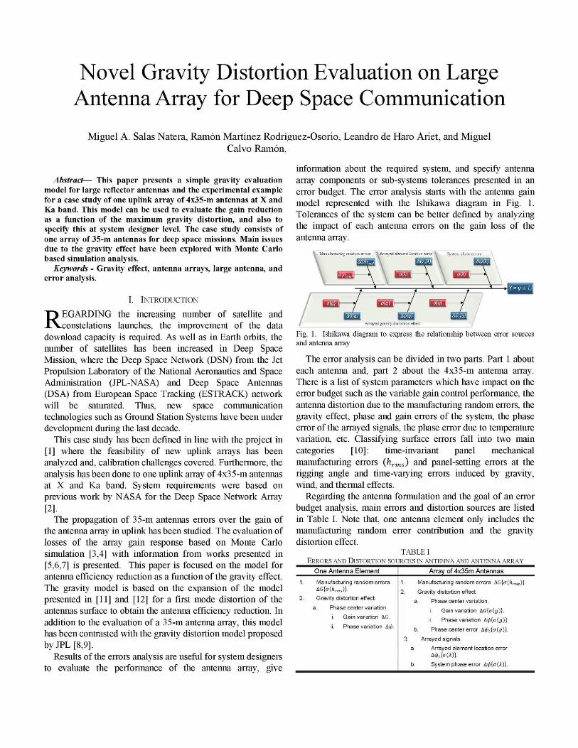
information about the required system, and specify antenna array components or sub-systems tolerances presented in an error budget. The error analysis starts with the antenna gain model represented with the Ishikawa diagram in Fig. 1. Tolerances of the system can be better defined by analyzing the impact of each antenna errors on the gain loss of the antenna array.
Fig. 1. Ishikawa diagram to express the relationship between error sources and antenna array
The error analysis can be divided in two parts. Part 1 about each antenna and, part 2 about the 4x35-m antenna array. There is a list of system parameters which have impact on the error budget such as the variable gain control performance, the antenna distortion due to the manufacturing random errors, the gravity effect, phase and gain errors of the system, the phase error of the arrayed signals, the phase error due to temperature variation, etc. Classifying surface errors fall into two main categories [10]: time-invariant panel mechanical manufacturing errors Qirms) and panel-setting errors at the rigging angle and time-varying errors induced by gravity, wind, and thermal effects.
Regarding the antenna formulation and the goal of an error budget analysis, main errors and distortion sources are listed in Table I. Note that, one antenna element only includes the manufacturing random error contribution and the gravity distortion effect.
TABLE I ERRORS AND DISTORTION SOURCES IN ANTENNA AND ANTENNA ARRAY
One Antenna Element
1. Manufacturing random errors AGiaih^)}.
2. Gravity distortion effect.
a. Phase center variation.
i. Gain variation AG.
ii. Phase variation AT/J.
Array of 4x35m Antennas
1. Manufacturing random errors AG{a(hrms)}.
2. Gravity distortion effect.
a. Phase center variation.
i. Gain variation AG{a(g)}.
ii. Phase variation Aip{a(g)}.
b. Phase center error AipL{a(g)}.
3. Arrayed signals.
a. Arrayed element location error A M f f W } .
b. System phase error AT/J{<T(/1)}.
The gravity model has been fitted for larger antenna dishes of 35-m diameter with a third order polynomial regression also applied for 6 and 12 m diameter antennas. Furthermore, the results from the gravity distortion evaluation have been contrasted with the JPL model in [8,9] obtaining good results.
This paper is organized as follows: Section II explains the model for evaluation of the gravity effect. Section III presents the results of the evaluation of the gravity effect on the case study. Finally, in section IV, conclusions of this work are listed.
II. GAIN VARIATION MODEL FOR GRAVITY EFFECT
The gravity model is based on the distortion model presented in [11,12] and presented in equation (1) for one antenna.
A Z : w 3(Mgcp) (1)
Where 8max is the peak error on the main reflector surface due to the gravity distortion. D is the diameter of the main reflector. Mg is the modal index related with the spatial variation of the distortion, p is the radial distance to the symmetry axis (z). Finally, cp is the angle between the vector of the radial distance and the X axis.
The gravity model with the first mode (Mg = 1) of distortion [13] has been fitted for larger antenna dishes of 35-m diameter with a third order polynomial equation. The equation (1) was solved for 6 and 12 meters antennas and GRASP (TICRA) simulations have been performed to obtain the efficiency reduction model then fitted for 35-m antennas.
The maximum gravity error emax for simulations in this work is 1.1 mm. Thus, the gravity distortion model for DSA 35-m antennas can be expressed in terms of the reduction of the antenna efficiency as presented in equations (2) and (3) for Ka and X band, respectively.
ATiaKa(smax) =-0.12578-s
0.08969 s max
2 + max '
0.006455 -s„
A r l a X ( S m a x ) = 5.027 x 10~4 •
0.00103 -s 2
(2)
(3)
- 0.000711 s„ -1
Following, equation (4) from [8] is used to generate gain versus elevation curves. The gain values are referenced to the feed horn aperture so different configurations will have the same gain values.
G(9) = G 0 - G 1 ( e - Y ) 2 A. s in (9 )
[dBi] (4)
Where y is the angle at which the antenna has been previously compensated for gravity distortion (y = 45 in this case study). For validation of the gravity model, G1 in equation (4) can be estimated as the ratio between the undistorted and the distorted antenna gain at Gant(90°) as follows
G i G 0 - G m t ( 9 0 ° )
(90 - y ) 2 (5)
Gant(90°) in term of the antenna efficiency reduction at e can be expressed as follows
G a n t ( 9 0 ° ) = 1 0 - l o g l 0 Tla -ATla(Smax)l «T A. i
(6)
G0 is the antenna peak gain calculated using the Ruze formula from [14].
G 0 = 1 0 . 1 o g l 0 K | ^ - 4 . 3 4 3 - p ^ (7)
III. RESULTS OF THE GRAVITY EFFECT EVALUATION
A. Validation of the proposed model for gravity effect
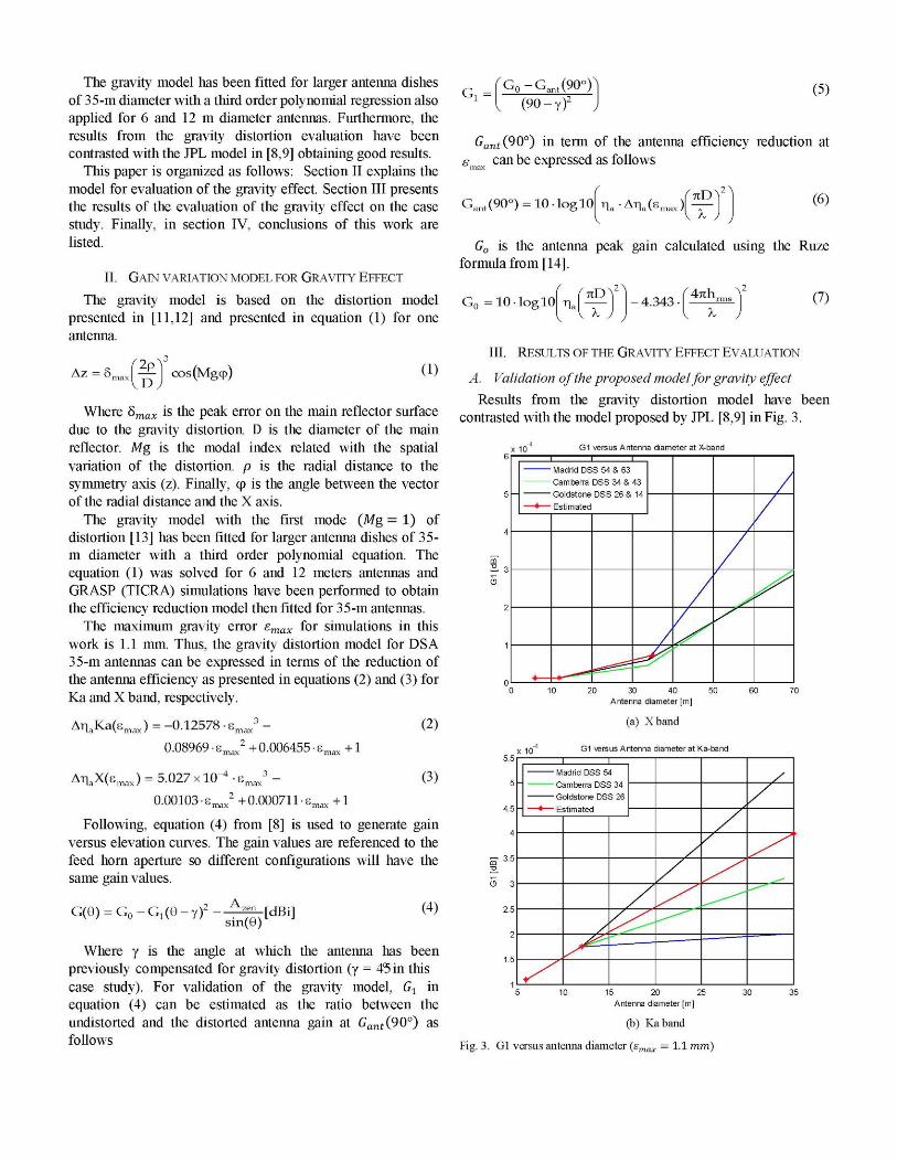
Results from the gravity distortion model have been contrasted with the model proposed by JPL [8,9] in Fig. 3.
y in" 4 G1 versus Antenna diameter at X-band 1 1 —
Fig. 3. Gl versus antenna diameter (smax = 1.1 mm)
Fig. 3 shows the validation of the third order equations proposed to estimate the reduction of the antenna efficiency contrasting Gl values of 34 and 70 m antennas of Madrid, Goldstone, and Camberra, to those Gl values of the analyzed antennas of 6, 12 [3], and the 35-m antennas of this case study.
The Gl value estimated for the 35-m antenna fulfills the expected Gl value of the proposed model by JPL as depicted in Fig. 3. Data for the 70 m diameter antenna has been found only for X band, while the 34-m diameter antenna has available data for X/Ka bands operating mode. Furthermore, results depicted in Fig. 3 shows good results also for the estimated Gl values of 6 and 12 meters antennas.
The gain G0 values of the undistorted 35-m antenna with hrms = 0 mm are 68.66 dBi (rja= 67.2%) and 79.83 dBi (rja= 61%) for X and Ka band, respectively.
B. Gain variation
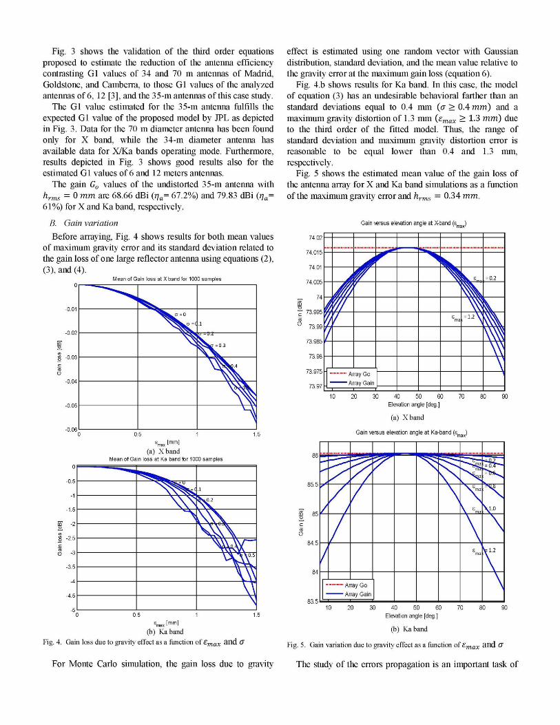
Before arraying, Fig. 4 shows results for both mean values of maximum gravity error and its standard deviation related to the gain loss of one large reflector antenna using equations (2), (3), and (4).
o
-0.01
M ean of Gain loss at X band for 1000 sam pies
.1
fcv^K"0,3
\S?^:4
0.5 1 s [mm] max L J
(a) Xband Mean of Gain loss at Ka band for 1000 samples
0
-0.5
-1
-1.5
m -2
in
8 -2.5
a -3
-3.5
-4
-4.5
-5
. i
N ^ . 2
V X \ \ r j . 5
emaxlmm]
(b) Kaband
Fig. 4. Gain loss due to gravity effect as a function oi£max and <7
For Monte Carlo simulation, the gain loss due to gravity
effect is estimated using one random vector with Gaussian distribution, standard deviation, and the mean value relative to the gravity error at the maximum gain loss (equation 6).
Fig. 4.b shows results for Ka band. In this case, the model of equation (3) has an undesirable behavioral farther than an standard deviations equal to 0.4 mm (a > 0.4 mm) and a maximum gravity distortion of 1.3 mm (emax > 1.3 mm) due to the third order of the fitted model. Thus, the range of standard deviation and maximum gravity distortion error is reasonable to be equal lower than 0.4 and 1.3 mm, respectively.
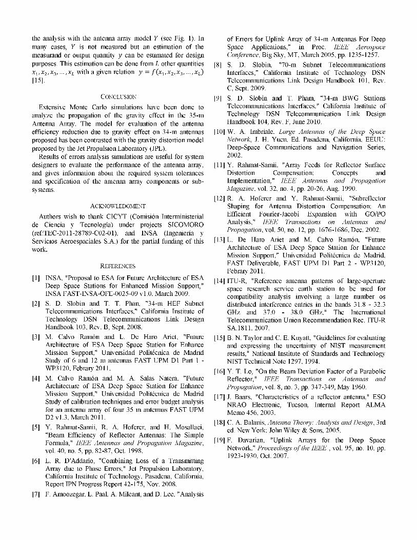
Fig. 5 shows the estimated mean value of the gain loss of the antenna array for X and Ka band simulations as a function of the maximum gravity error and hrms = 0.34 mm.
74.02
74.015
74.01
74.005
74
73.995
73.99
73.985
73.98
73.975
73.97
Ar
Ar
ray Go
ray Gain i i
s ma
SW s—
= 12 \
= 0.2
10 20 30 40 50 6 Elevation angle [deg.]
(a) Xband
70 90
85.5
m 85
84.5
83.5 A
— i
ray Go
ray Gain
^ ^ mS
^¡ijna
V ma
s ma
Toí—
\ l . O
^1.2
10 20 30 40 50 6
Elevation angle [deg.]
70 80 90
(b) Kaband
Fig. 5. Gain variation due to gravity effect as a function of £max and <7
The study of the errors propagation is an important task of
the analysis with the antenna array model Y (see Fig. 1). In many cases, Y is not measured but an estimation of the measurand or output quantity y can be estimated for design purposes. This estimation can be done from L other quantities x±, x2, x3,..., xL with a given relation y = f(x±, x2, x3,..., xL) [15].
CONCLUSION
Extensive Monte Carlo simulations have been done to analyze the propagation of the gravity effect in the 35-m Antenna Array. The model for evaluation of the antenna efficiency reduction due to gravity effect on 34-m antennas proposed has been contrasted with the gravity distortion model proposed by the Jet Propulsion Laboratory (JPL).
Results of errors analysis simulations are useful for system designers to evaluate the performance of the antenna array, and gives information about the required system tolerances and specification of the antenna array components or subsystems.
ACKNOWLEDGMENT
Authors wish to thank CICYT (Comisión Interministerial de Ciencia y Tecnología) under projects SICÓMORO (ref:TEC-2011-28789-C02-01), and INSA (Ingeniería y Servicios Aeroespaciales S.A.) for the partial funding of this work.
REFERENCES
[1] INSA, "Proposal to ESA for Future Architecture of ESA Deep Space Stations for Enhanced Mission Support," INSA FAST-INSA-OFE-0025-09 vl.O, March 2009.
[2] S. D. Slobin and T. T. Phan, "34-m HEF Subnet Telecommunications Interfaces," California Institute of Technology DSN Telecommunications Link Design Handbook 103, Rev. B, Sept. 2008.
[3] M. Calvo Ramón and L. De Haro Ariet, "Future Architecture of ESA Deep Space Station for Enhance Mission Support," Universidad Politécnica de Madrid Study of 6 and 12 m antennas FAST UPM Dl Part 1 -WP3120,Febrary2011.
[4] M. Calvo Ramón and M. A. Salas Natera, "Future Architecture of ESA Deep Space Station for Enhance Mission Support," Universidad Politécnica de Madrid Study of calibration techniques and error budget analysis for an antenna array of four 35 m antennas FAST UPM D2vl.3, March 2011.
[5] Y. Rahmat-Samii, R. A. Hoferer, and H. Mosallaei, "Beam Efficiency of Reflector Antennas: The Simple Formula," IEEE Antennas and Propagation Magazine, vol. 40, no. 5, pp. 82-87, Oct. 1998.
[6] L. R. D'Addario, "Combining Loss of a Transmitting Array due to Phase Errors," Jet Propulsion Laboratory, California Institute of Technology, Pasadena, California, Report IPN Progress Report 42-175, Nov. 2008.
[7] F. Amoozegar, L. Paal, A. Mileant, and D. Lee, "Analysis
of Errors for Uplink Array of 34-m Antennas For Deep Space Applications," in Proc. IEEE Aerospace Conference, Big Sky, MT, March 2005, pp. 1235-1257.
[8] S. D. Slobin, "70-m Subnet Telecommunications Interfaces," California Institute of Technology DSN Telecommunications Link Design Handbook 101, Rev. C, Sept. 2009.
[9] S. D. Slobin and T. Pham, "34-m BWG Stations Telecommunications Interfaces," California Institute of Technology DSN Telecommunication Link Design Handbook 104, Rev. F, June 2010.
[10] W. A. Imbriale, Large Antennas of the Deep Space Network, J. H. Yuen, Ed. Pasadena, California, EEUU: Deep-Space Communications and Navigation Series, 2002.
[11] Y. Rahmat-Samii, "Array Feeds for Reflector Surface Distortion Compensation: Concepts and Implementation," IEEE Antennas and Propagation Magazine, vol. 32, no. 4, pp. 20-26, Aug. 1990.
[12] R. A. Hoferer and Y. Rahmat-Samii, "Subreflector Shaping for Antenna Distortion Compensation: An Efficient Fourier-Jacobi Expansion with GO/PO Analysis," IEEE Transactions on Antennas and Propagation, vol. 50, no. 12, pp. 1676-1686, Dec. 2002.
[13] L. De Haro Ariet and M. Calvo Ramón, "Future Architecture of ESA Deep Space Station for Enhance Mission Support," Universidad Politécnica de Madrid, FAST Deliverable, FAST UPM Dl Part 2 - WP3120, Febrary2011.
[14] ITU-R, "Reference antenna patterns of large-aperture space research service earth station to be used for compatibility analysis involving a large number os distributed interference entries in the bands 31.8 - 32.3 GHz and 37.0 - 38.0 GHz," The International Telecommunication Union Recommendation Rec. ITU-R SA.1811,2007.
[15] B. N. Taylor and C. E. Kuyatt, "Guidelines for evaluating and expressing the uncertainty of NIST measurement results," National Institute of Standards and Technology NIST Technical Note 1297, 1994.
[16] Y. T. Lo, "On the Beam Deviation Factor of a Parabolic Reflector," IEEE Transactions on Antennas and Propagation, vol. 8, no. 3, pp. 347-349, May 1960.
[17] J. Baars, "Characteristics of a reflector antenna," ESO NRAO Electronic, Tucson, Internal Report ALMA Memo 456, 2003.
[18] C. A. Balarás, Antenna Theory: Analysis and Design, 3rd ed. New York: John Wiley & Sons, 2005.
[19] F. Davarian, "Uplink Arrays for the Deep Space Network," Proceedings of the IEEE , vol. 95, no. 10, pp. 1923-1930, Oct. 2007.