NOVEL NUMERICAL METHODS FOR SOLVING THE TIME-SPACEFRACTIONAL DIFFUSION EQUATION IN TWO DIMENSIONS∗
QIANQIAN YANG† , IAN TURNER† , FAWANG LIU† , AND MILOS ILIC†
Abstract. In this paper, a time-space fractional diffusion equation in two dimensions (TSFDE-2D) with homogeneous Dirichlet boundary conditions is considered. The TSFDE-2D is obtainedfrom the standard diffusion equation by replacing the first-order time derivative with the Caputofractional derivative tD
γ∗ , γ ∈ (0, 1), and the second-order space derivatives with the fractional
Laplacian −(−Δ)α/2, α ∈ (1, 2]. Using the matrix transfer technique proposed by Ilic et al. [M. Ilic,F. Liu, I. Turner, and V. Anh, Fract. Calc. Appl. Anal., 9 (2006), pp. 333–349], the TSFDE-2Dis transformed into a time fractional differential system as tD
γ∗u = −KαAα/2u, where A is the
approximate matrix representation of (−Δ). Traditional approximation of Aα/2 requires diagonal-ization of A, which is very time-consuming for large sparse matrices. The novelty of our proposednumerical schemes is that, using either the finite difference method or the Laplace transform tohandle the Caputo time fractional derivative, the solution of the TSFDE-2D is written in terms ofa matrix function vector product f(A)b at each time step, where b is a suitably defined vector.Depending on the method used to generate the matrix A, the product f(A)b can be approximatedusing either the preconditioned Lanczos method when A is symmetric or the M-Lanzcos methodwhen A is nonsymmetric, which are powerful techniques for solving large linear systems. We giveerror bounds for the new methods and illustrate their roles in solving the TSFDE-2D. We also derivethe analytical solution of the TSFDE-2D in terms of the Mittag–Leffler function. Finally, numericalresults are presented to verify the proposed numerical solution strategies.
Key words. fractional calculus, Caputo fractional derivative, fractional Laplacian, finite differ-ence method, finite element method, matrix transfer technique, Lanczos method, M-Lanczos method,matrix function
1. Introduction. During the past three decades, the subject of fractional cal-culus (that is, calculus of integrals and derivatives of arbitrary order) has gainedconsiderable popularity and importance, mainly due to its demonstrated applicationsin numerous diverse and widespread fields in science, engineering, and finance. Forexample, fractional calculus has been successfully applied to problems in system bi-ology [55], physics [2, 18, 35, 36, 41, 56], chemistry and biochemistry [54], hydrology[3, 4, 29], medicine [16, 17, 32], and finance [14, 34, 38, 44, 51].
A number of numerical methods have now been proposed for solving the time, orspace, or time-space fractional partial differential equations. A literature review ofthese numerical methods can be found in the first author’s Ph.D. thesis [52]. To datethe dominant numerical methods for solving fractional PDEs are based on the finitedifference method. However, because the fractional derivative is a nonlocal operator,it is challenging to harness the long history involving classical numerical techniques,such as the finite element method, the finite volume method, or the new mesh-freemethod, to solve fractional PDEs. This paper makes an important contribution to
∗Submitted to the journal’s Computational Methods in Science and Engineering section June 30,2010; accepted for publication (in revised form) February 28, 2011; published electronically May19, 2011. This research has been supported by an ARC grant DP0986766, a Ph.D. Fee WaiverScholarship, and a School of Mathematical Sciences Scholarship at QUT.
http://www.siam.org/journals/sisc/33-3/80063.html†Discipline of Mathematical Sciences, Queensland University of Technology, GPO Box
the literature by expressing the solution in terms of a matrix function vector productat each time step utilizing the matrix transfer technique. This enables the prevailingLanczos method to be used for the required matrix functions.
To elucidate these ideas, we consider the following time-space fractional diffu-sion equation in two dimensions (TSFDE-2D) with homogeneous Dirichlet boundaryconditions and given initial condition
tDγ∗u(x, y, t) = −Kα(−Δ)α/2u(x, y, t),(1.1)
u(0, y, t) = u(a, y, t) = 0,(1.2)
u(x, 0, t) = u(x, b, t) = 0,(1.3)
u(x, y, 0) = u0(x, y),(1.4)
where the Laplacian operator is defined as −Δ = − ∂2
∂x2 − ∂2
∂y2 ; u is, for example, a
solute concentration; and Kα represents the diffusion coefficient. tDγ∗ is the Caputo
fractional derivative of order γ (0 < γ < 1) with respect to t and with the startingpoint at t = 0 defined as [37]
(1.5) tDγ∗u(x, y, t) =
1
Γ(1− γ)
∫ t
0
ut(x, y, τ)
(t− τ)γdτ.
The symmetric space fractional derivative −(−Δ)α/2 of order α (1 < α ≤ 2) is afractional Laplacian operator defined through the eigenfunction expansion on a finitedomain (see Definition 2.1 or [22]).
We remark that there is another definition for the fractional Laplacian operatorgiven in the literature, utilizing the Fourier transform on an infinite domain [42], witha natural extension to finite domains when the function is subject to homogeneousDirichlet boundary conditions. It is essential to choose an appropriate numericalmethod of approximation according to which definition is intended. Yang, Liu, andTurner [53] show that using this alternative definition, the one-dimensional fractionalLaplacian operator −(−Δ)α/2 is equivalent to the Riesz fractional derivative ∂α
∂|x|αunder homogeneous Dirichlet boundary conditions and hence can be approximatedby the standard/shifted Grunwald method and the L1/L2 approximation.
Hilfer [19] argues that the fractional Laplace equation with the Riesz spatialfractional derivative breaches the principle of locality in physics. The reason for thisis that the Riesz fractional derivative is defined by using a Fourier transform on allspace and cannot accommodate boundary conditions on finite domains (or if one doesimpose boundary conditions, they are artificial). In our case we define the fractionalpower of an operator using the spectral decomposition on a finite domain with givenboundary conditions so that the interior/exterior problems (raised by Hilfer) cannotoccur. In our context, although the operator is nonlocal, the effect is confined tothe domain of concern, the same as a Fourier series represents a function on itsfundamental domain but is periodically extended elsewhere. Reasonably good resultshave been obtained using our modeling in drying porous media [48], and similarlygood results have been reported by Benson, Wheatcraft, and Meerschaert [3, 4].
To solve the TSFDE-2D (1.1)–(1.4), we first introduce a mesh and discretize inspace using either the finite difference or finite element method to obtain an approx-imate matrix representation A of the Laplacian (−Δ). Using the matrix transfertechnique proposed by Ilic et al. [22], the TSFDE-2D is transformed into a time frac-tional differential system involving the matrix A raised to the fractional index α/2
We then propose two numerical schemes to solve this equation using either the finitedifference method or the Laplace transform to handle the Caputo time fractionalderivative, which necessitates the computation of a matrix function vector productf(A)b at each time step, where b is a suitably defined vector. We show how thisproduct can be approximated and give algorithms for each scheme that can easily beadapted for MATLAB.
The rest of this paper is organized as follows. In section 2, we present twonovel numerical schemes to simulate the solution behavior of the TSFDE-2D (1.1)–(1.4). In section 3, to approximate the product f(A)b involved in the two numericalschemes, the adaptively preconditioned Lanczos method when A is symmetric andthe incomplete Cholesky preconditionedM-Lanzcos method when A is nonsymmetricare presented. In section 4, error bounds for the two newly proposed numericalschemes are derived. The analytical solution of the TSFDE-2D is derived in section 5.Finally, numerical experiments are carried out in section 6 to assess the computationalperformance and accuracy of our new schemes, and some conclusions are drawn insection 7.
2. Numerical schemes for the TSFDE-2D. In this section, we present twonumerical schemes to simulate the solution behavior of the TSFDE-2D (1.1)–(1.4).In section 2.1, the matrix transfer technique is introduced to discretize the fractionalLaplacian. In section 2.2, a finite difference method is used to discretize the Caputotime fractional derivative. Section 2.3 shows how the first numerical scheme is derived,by combining the finite difference method and the matrix transfer technique to transferthe TSFDE-2D (1.1)–(1.4) into a discrete system describing the evolution of u(x, y, t)in space and time. Finally, in section 2.4, the second numerical scheme is presented,which is exact in time, by employing the Laplace transform together with the matrixtransfer technique.
2.1. Matrix transfer technique in space. We utilize the matrix transfer tech-nique proposed by Ilic et al. [21, 22] to discretize in space. In this paper the symbol(−Δ)α/2 has the usual meaning as a function of (−Δ), which is defined in terms ofits spectral decomposition. For boundary value problems on finite domains, discreteeigenfunction expansions are used, where the following definition is adopted.
Definition 2.1 (see [22]). Suppose the two-dimensional (2D) Laplacian (−Δ)has a complete set of orthonormal eigenfunctions ϕn,m corresponding to eigenvaluesλn,m in a rectangular region D = {(x, y)|0 ≤ x ≤ a, 0 ≤ y ≤ b}, i.e., (−Δ)ϕn,m =λn,mϕn,m, B(ϕ) = 0 on ∂D, where B(ϕ) is the homogeneous Dirichlet boundary con-dition. Let
Fη =
{f =
∞∑n=1
∞∑m=1
cn,mϕn,m, cn,m = 〈f, ϕn,m〉,∞∑
n=1
|cn,m|2|λn,m|α < ∞, 1 < α ≤ 2
};
then for any f ∈ Fη, the 2D fractional Laplacian (−Δ)α/2 is defined by
One notes that the fractional Laplacian (−Δ)α/2 is a nonlocal operator and anyapproximation of it will therefore result in a large dense matrix. One of the attractiveadvantages of the matrix transfer technique is the fact that the sparse approximationof (−Δ) can be harnessed directly in the numerical solution technique, which we nowexplain.
By introducing a mesh and denoting the value of u(x, y, t) at the ith node byui(t), and the vector of such values by u(t), the matrix transfer technique for solvingthe TSFDE-2D (1.1)–(1.4) proceeds by first considering the nonfractional equation
du
dt= −Au,(2.1)
where A is the approximate matrix representation of the standard Laplacian (−Δ)under homogeneous Dirichlet boundary conditions, obtained by using either finitedifference or finite element methods. Clearly, (−Δ) is an unbounded operator, whereasA is a bounded matrix operator and therefore it is not possible to conclude that A isa good representation of (−Δ). However, the resolvents of each operator are bounded,and this motivates the thinking that A is a good approximate representation of (−Δ).Further discussion on this observation can be found in Simpson [47], which followsthe fundamental ideas of convergence of the integral representation of Aα/2 given inMatsuki and Ushijima [33]. Then under the matrix transfer technique, the fractionalLaplacian operator is approximated as
(2.2) −(−Δ)α/2u ≈ −Aα/2u.
In summary, the matrix transfer technique transforms the TSFDE-2D (1.1)–(1.4) intothe following time fractional differential system:
tDγ∗u = −KαA
α/2u.(2.3)
This method enables the standard finite difference or finite element methods to beutilized for the spatial discretization of the Laplacian operator, which we now describein sections 2.1.1 and 2.1.2, respectively.
2.1.1. Finite difference method in space. The standard five-point finite dif-ference stencil with equal grid spacing in both x and y directions, i.e., h = a
M = bN ,
will result in the block tridiagonal approximate matrix representation of the Lapla-cian, namely,
A =1
h2
⎡⎢⎢⎢⎢⎢⎣B −I−I B −I
. . .. . .
. . .
−I B −I−I B
⎤⎥⎥⎥⎥⎥⎦ with B =
⎡⎢⎢⎢⎢⎢⎣4 −1−1 4 −1
−1 4 −1. . .
. . . −1−1 4
⎤⎥⎥⎥⎥⎥⎦ ,
(2.4)
where A ∈ R(M−1)(N−1)×(M−1)(N−1) and B ∈ R(M−1)×(M−1).
2.1.2. Finite element method in space. In the case of the finite elementmethod, we begin with the following nonfractional governing equation:
for a 2D domain Ω = [0, a]× [0, b]. The boundary conditions are
u = 0 on ∂Ω.(2.6)
Multiplying (2.5) by a test function v and integrating over the computational domainΩ gives ∫
Ω
∂u
∂tv dΩ = −
∫Ω
(−Δ)u v dΩ.(2.7)
In order to develop the weak form of (2.7), integration by parts is applied to theright-hand side to reduce the order of differentiation within the integral. Requiringthat the test function v vanishes on ∂Ω, we obtain the weak form∫
Ω
∂u
∂tv dΩ = −
∫Ω
∇u · ∇v dΩ.(2.8)
Discretization of the domain in (2.8) is performed using three-node triangular ele-ments, which are also known as the linear triangular elements [25, 30].
Expanding u(x, y, t) in terms of the shape functions {φi(x, y)}Ni=1, we obtain
u(x, y, t) =
N∑i=1
ui(t)φi(x, y),(2.9)
where N is the number of free nodes in the mesh. We note from (2.9) that the shapefunctions are used to interpolate the spatial variation, while the temporal variation isrelated to the nodal variables.
We take v = φj , j = 1, . . . ,N , in (2.8) and obtain the discrete formulation∫Ω
N∑i=1
dui
dtφi φj dΩ = −
∫Ω
N∑i=1
ui∇φi · ∇φj dΩ, j = 1, . . . ,N ,(2.10)
or, upon interchanging summation and integration,
N∑i=1
dui
dt
∫Ω
φi φj dΩ = −N∑i=1
ui
∫Ω
∇φi · ∇φj dΩ, j = 1, . . . ,N .(2.11)
Introducing the “mass” matrix (M)ij =∫Ω φiφj dΩ and the “stiffness” matrix (K)ij =∫
Ω∇φi · ∇φj dΩ, (2.11) can be written as
du
dt= −M−1Ku.(2.12)
Thus, we have derived that the approximate matrix representation of the standardLaplacian for the finite element method is
A = M−1K.(2.13)
Interestingly, although both M and K are symmetric positive definite and sparse, A isnot only nonsymmetric, it is also dense. Nevertheless, a standard argument in linearalgebra shows that A is similar to the symmetric positive matrix A = M− 1
2KM− 12 ,
and therefore its eigenvalues are positive and real, and hence A itself is positivedefinite, as is stated in the following proposition.
Proposition 2.2. The matrix A = M−1K is similar to the symmetric positivematrix A = M− 1
2.2. Finite difference method in time. We now discretize (2.3) in time usingthe following scheme. Define tn := nτ, n = 0, 1, 2, . . . , where τ is the time step. Weadopt the finite difference method (FDM) to discretize the Caputo time fractionalderivative as [28]
tDγ∗u
n =1
μ0
n−1∑j=0
bj [un−j − un−1−j] +O(τ2−γ),(2.14)
where μ0 = τγΓ(2− γ), bj = (j + 1)1−γ − j1−γ , j = 0, 1, 2, . . . , n− 1.One difficulty with this approach, and indeed in solving time fractional differential
equations in general, is that the fractional derivatives are nonlocal operators. Thisnonlocal property means that the next state of the system depends not only on itscurrent state but also on the historical states starting from the initial time. Hence,applying the scheme (2.14) requires the storage and processing of all previous timesteps. In this work, we assume that the additional memory and computational costis acceptable. However, we note that some authors have explored techniques forreducing this cost (see, e.g., Podlubny [37], Ford and Simpson [13], Diethelm et al.[6], and Deng [5]).
2.3. Scheme 1: Finite difference method with matrix transfer tech-nique. Combining the approximation for the Caputo time fractional derivative (2.14)with the approximation of the fractional Laplacian (2.2), we obtain the following nu-merical approximation of the TSFDE-2D (1.1)–(1.4):
1
μ0
n−1∑j=0
bj [un−j − un−1−j ] = −KαA
α/2un.(2.15)
After some further manipulations, (2.15) reads
un =[I+ μ0KαA
α/2]−1
⎡⎣n−2∑j=0
(bj − bj+1)un−1−j + bn−1u
0
⎤⎦ .(2.16)
Defining the scalar function f1(ξ) =[1 + μ0Kαξ
α/2]−1
, we obtain the first numericalscheme for approximating the TSFDE-2D (1.1)–(1.4) as
un = f1(A)b1n, with b1
n =n−2∑j=0
(bj − bj+1)un−1−j + bn−1u
0,(2.17)
where A is generated using either the finite difference method (2.4) or the finiteelement method (2.13), u0 is the discrete representation of the initial value u0(x, y),and μ0 and bj are defined in section 2.2.
2.4. Scheme 2: Exact-in-time method with matrix transfer technique.We now consider an alternative strategy for approximating the fractional differentialsystem (2.3) associated with the TSFDE-2D (1.1). Taking the Laplace transform of(2.3) with un = L{un(t)} yields
where Λ = diag(λi, i = 1, . . . ,m), λi being the eigenvalues of A, then from (2.19) weobtain
un = L−1
{[sI+ s1−γKαA
α/2]−1
u0
}= Pdiag
{L−1
{1
s+ s1−γKαλα/2i
}, i = 1, . . . ,m
}P−1u0.(2.21)
To perform the required inversion we require the Mittag–Leffler function Eγ(z) [37],
Eγ(z) =
∞∑k=0
zk
Γ(γk + 1),(2.22)
which is a generalization of the exponential function, with Laplace transform givenby
L{Eγ(−ωtγ)} =1
s+ s1−γω, (s) > |ω|1/γ .(2.23)
Using (2.23), we obtain
un = Pdiag{Eγ(−Kαλ
α/2i tγn), i = 1, . . . ,m
}P−1u0(2.24)
= Eγ(−KαAα/2tγn)u
0.(2.25)
Defining the scalar function f2(ξ) = Eγ
(−Kαξα/2tγn
), we obtain the second numerical
scheme for approximating the TSFDE-2D (1.1)–(1.4) as
un = f2(A)b2, with b2 = u0.(2.26)
We refer to (2.17) and (2.26) as Schemes 1 and 2 throughout the remaining sectionsof this paper. In section 3, we show how these numerical schemes can be implementedusing either the Lanczos method (A is generated from the finite difference method)or the M-Lanczos method (A is generated from the finite element method).
3. Matrix function approximation and solution strategy. In this section,we devise efficient algorithms to approximate the matrix function vector productsf1(A)b1
n, f2(A)b2 for Schemes 1 and 2 in section 2.3 and section 2.4, respectively.The prevailing method in the literature for approximating the matrix-vector prod-
uct f(A)b for a scalar, analytic function f(t) : D ⊂ C → C is the Lanczos approxi-mation
is the Lanczos decomposition, the columns of Vm form an orthonormal basis for theKrylov subspace Km(A,b) = span{b,Ab, . . . ,Am−1b}, and Tm is symmetric andtridiagonal. This approximation has been considered by van der Vorst [50], Saad [39],Druskin and Knizhnerman [7], Hochbruck and Lubich [20], Sidje [45], van den Eshofet al. [49], Eiermann and Ernst [8], Lopez and Simoncini [31], Ilic, Turner, and Anh[23], and Ilic, Turner, and Simpson [24] as well as many other researchers during thelast twenty years.
The standard Lanczos method requires that the matrix A must be symmetric.Although the matrix A generated from the finite difference method is symmetric,A generated from the finite element method is nonsymmetric. Therefore, we needdifferent approximation strategies for the numerical schemes depending on the methodused to generate the matrix A.
3.1. Lanczos method with an adaptive preconditioner. In this section,we assume the matrix A is generated from the finite difference method, as illustratedin section 2.1, and hence is symmetric. Thus, we can use the standard Lanczosmethod. Memory constraints often require restarting the Lanczos decomposition;however, this is not straightforward in the context of matrix function approximation.To improve convergence of the Lanczos approximation, in this section, we use anadaptively preconditioned Lanczos method [23].
First, using Lehoucq and Sorensen’s implicitly restarted Arnoldi method [27], wecompute the k smallest eigenvalues {θi}ki=1 and corresponding eigenvectors {qi}ki=1
of the matrix A. Setting Qk = [q1,q2, . . . ,qk] and Λk = diag{θ1, . . . , θk}, the pre-conditioner Z−1 takes the form
Z−1 = θ∗QkΛ−1k QT
k + I−QkQTk ,
where θ∗ = θmin+θmax
2 . Here θmin, θmax are the smallest and largest eigenvaluesof A, respectively, obtained from the implicit restarted Arnoldi process [39]. Thispreconditioner eliminates the influence of the k smallest eigenvalues of A on the rateof convergence of the standard Lanczos method. The matrix AZ−1 has the sameeigenvectors as A; however, its eigenvalues {λi}ki=1 are shifted to θ∗ [1, 11]. We nowshow how this spectral information can be used to aid with the approximation ofun = f(A)b.
The important observation at this point is the following relationship betweenf(A) and f(AZ−1).
Proposition 3.1 (see [23]). Let span{q1,q2, . . . ,qk} be an eigenspace of a sym-metric matrix A such that AQk = QkΛk, with Qk = [q1,q2, . . . ,qk] and Λk =diag(θ1, . . . , θk). Define Z = 1
θ∗QkΛkQTk + I−QkQ
Tk ; then for v ∈ Rn
f(A)v = Qkf(Λk)QTk v + f(AZ−1)(I−QkQ
Tk )v.
Using Proposition 3.1, we can approximate un = f(A)b as
f(A)b = Qkf(Λk)QTk b+ f(AZ−1)b,(3.3)
where b = (I − QkQTk )b. Note that if A is symmetric positive definite, then so is
AZ−1. Hence, we can apply the standard Lanczos decomposition to AZ−1, i.e.,
where v1 = b/‖b‖. Next perform the spectral decomposition of Tm = YmΛmYTm
and set Qm = VmYm; then compute the Lanczos approximation
(3.4) f(AZ−1)b ≈ Vmf(Tm)VTmb = Qmf(Λm)QT
mb.
Based on the theory presented to this point, we propose the following algorithm toapproximate the solution of the TSFDE-2D (1.1).
Algorithm 3.1: Lanczos approximation to f1(A)bn1 , f2(A)b2 with adaptive
preconditioning, where A is symmetric positive definite.Input: Discrete Laplacian matrix A, right-hand side vector b, tolerance τ , order of spatial
derivative α, order of temporal derivative γ, number of time steps n, number ofstored Ritz pairs k, and maximum size of Krylov subspace maxiter.
Output: un
Compute Λk and Qk to construct preconditioner Z−1;for time step j = 1 : n do
Set b = (I −QkQTk )b;
Set v1 = b/‖b‖2;for m = 1 : maxiter do
Set q = AZ−1vm;if m �= 1 then
q = q − βm−1vm−1;end
αm = vTmq;q = q − αmvm;βm = ‖q‖2;vm+1 = q/βm;
Compute linear system residual ‖rm‖2 = ‖b‖2 |βmeTmT−1m e1|;
Compute μmin – the smallest eigenvalue of Tm;For Scheme 1, compute error bound as f(μmin)‖rm‖2;For Scheme 2, compute error bound as 1
π
∫∞0
|�Eγ(−Kαζα/2tγneiπα/2)|dζμmin+ζ
‖rm‖2;if error bound < τ then
break;end
end
Compute uj = Qkf(Λk)QTk b+ ‖b‖2Vmf(Tm)e1;
end
Remark 3.1. In Algorithm 3.1, the preconditioner Z−1 does not need to beexplicitly formed, since it can be applied in a straightforward manner from the storedlocked Ritz pairs Qk and Λk. These matrices are computed using MATLAB’s eigsfunction.
Remark 3.2. In Algorithm 3.1, the error bounds for approximating f1(A)bn1 ,
f2(A)b2, where A ∈ SPD, are derived in section 4. To compute the error bound forScheme 2, one needs to approximate an indefinite integral for a given time. To do this,we first evaluate |�Eγ(·)| in the integrand using the MATLAB code mlf.m developedby Podlubny.1 The integral is then computed using MATLAB’s quadgk function,which is developed based on the adaptive Gauss–Kronrod quadrature formula andallows the case where the integral limit is infinity to be evaluated. Our findings fromnumerical experimentation indicate that when α + γ ≥ 2, convergence issues arisewith the evaluation of Eγ(·). Similar problems are also discussed in [15]. We have
1This code can be found at http://www.mathworks.com/matlabcentral/fileexchange/8738.
Algorithm 3.2: M−Lanczos approximation to f1(M−1K)bn
1 , f2(M−1K)b2,
where M and K are symmetric positive definite matrices.Input: Mass matrix M, Stiffness matrix K, right-hand side vector b, tolerance τ , order of
spatial derivative α, order of temporal derivative γ, number of time steps n, andmaximum size of Krylov subspace maxiter.
Output: un
for time step j = 1 : n do
Set ρ =√bTMb;
Set v1 = b/ρ;for m = 1 : maxiter do
Set q = M−1Kvm;if m �= 1 then
q = q − βm−1vm−1;end
αm = vTmMq;q = q − αmvm;
βm =√
qTMq;vm+1 = q/βm;Compute linear system residual ‖rm‖2 = ρ‖vm+1‖2|βmeTmT−1
m e1|;Compute θmin – the smallest eigenvalue of A;
For Scheme 1, compute error bound as κ2(M12 )f(θmin)‖rm‖2;
For Scheme 2, compute error bound as
κ2(M12 )
π
∫ ∞0
|�Eγ(−Kαζα/2tγneiπα/2)|dζθmin+ζ
‖rm‖2;if error bound < τ then
break;end
end
Compute uj = ρVmf(Tm)e1;end
proved that absolute convergence of the integral in the Stieltjes transform requiresthat α + γ < 2 (see Proposition 4.5). Whether other possibilities hold needs furtherinvestigation, which we intend to pursue in future research.
Remark 3.3. In Algorithm 3.1, the smallest eigenvalue λmin of AZ−1 is approx-imated by the smallest eigenvalue μmin of Tm.
3.2. M-Lanczos method with an incomplete Cholesky preconditioner.In section 2.1.2, we saw that the approximate matrix representation of the Laplaciancorresponding to the finite element method was nonsymmetric. In this section, weinvestigate the matrix function approximations based on the Arnoldi decompositionin the M−inner product 〈x,y〉M = xTMy. The M-Arnoldi decomposition is wellknown in the context of solving nonsymmetric linear systems [46]. Essai [12] showedthat the M-Arnoldi decomposition is of the form
AVm = VmHm + βmvm+1eTm,
where the columns of Vm form a basis for Km(A,b), VTmMVm = I and Hm =
VTmMAVm is an m×m upper Hessenberg matrix.The advantage of using the M−inner product is that, as A is M–self-adjoint, Hm
is a symmetric tridiagonal matrix and the M-Arnoldi decomposition can be replacedwith the M-Lanczos decomposition
Using the M-Lanczos decomposition, we can define the M-Lanczos approximation tof(A)b as
f(A)b ≈ ‖b‖MVmf(Tm)e1,(3.5)
where ‖b‖M =√〈b,b〉M.
The algorithm for the M-Lanczos decomposition is given in Algorithm 3.2, whichis identical to the standard Lanczos approximation with every norm and inner productreplaced with the M-norm and the M−inner product.
Remark 3.4. In Algorithm 3.2, the evaluation of M−1Kvm is done by solvingMq = Kvm using the conjugate gradient method preconditioned with an incom-plete Cholesky factorisation. We use MATLAB functions pcg and cholinc for thispurpose.
Remark 3.5. In Algorithm 3.2, the error bounds for approximating f1(A)b1,f2(A)b2, where A = M−1K is nonsymmetric, are derived in section 4. The numericalevaluation of the integral in the error bound for Scheme 2 is discussed in Remark 3.2.
Remark 3.6. In Algorithm 3.2, κ2(M12 ) is the 2-norm condition number of M
12 ,
computed using MATLAB’s condest function.Remark 3.7. In Algorithm 3.2, the smallest eigenvalue θmin of A can be ei-
ther computed using MATLAB’s eigs function or taken as θmin = 2π2, which is anapproximation of the smallest eigenvalue of the Laplacian operator [9].
4. Error bounds for the numerical schemes. In this section, we derive theerror bounds used in Algorithms 3.1 and 3.2 for the two new numerical schemes andillustrate their roles in solving the TSFDE-2D (1.1)–(1.4).
First, we will show that both functions fk (k = 1, 2) can be written in the form
fk(ξ) =
∫ ∞
0
gk(ζ)dζ
ξ + ζ, ξ > 0,(4.1)
such that∫∞0
gk(ζ)dζξ+ζ is absolutely integrable. Equation (4.1) is known as a Stieltjes
integral equation [10].When A ∈ SPD, the following proposition gives the error in approximating
fk(A)b (k = 1, 2) by the Lanczos approximation (3.1) when fk(ξ) is expressible inthe form (4.1). In this section, unless otherwise stated, ‖ · ‖ represents the 2-norm.
Proposition 4.1. Define rm as the residual in solving Ax = b using m steps ofthe full orthogonalization method (FOM) [40]; then
Note that if A ∈ SPD, then AZ−1 ∈ SPD, where Z−1 is discussed in section 3.1.Thus, AZ−1 can be orthogonally diagonalized with its smallest eigenvalue λmin, andusing the result from [49, 23] that∣∣∣∣eTm(Tm + ζIm)−1e1
eTmT−1m e1
∣∣∣∣ < 1,
the error bound for the Lanczos approximation (3.4) can be written as
‖ε(k)m ‖ ≤∫ ∞
0
|gk(ζ)|λmin + ζ
dζ ‖rm‖, k = 1, 2.
In the case where A = M−1K is positive definite (see Proposition 2.2) and fk(ξ)is expressed in the form (4.1), we have the following proposition for defining the errorin approximating fk(A)b (k = 1, 2) by the M-Lanczos approximation (3.5).
Proposition 4.2. Define rm as the residual in solving Ax = b using M-weightedFOM [12] by rm = −‖b‖M βm(eTmT−1
m e1)vm+1; then
ε(k)m :=fk(A)b− ‖b‖MVmfk(Tm)e1
=
∫ ∞
0
gk(ζ) (A + ζI)−1
(eTm(Tm + ζIm)−1e1
eTmT−1m e1
)rm dζ.
Proof. Proceeding as in Proposition 4.1, we have
fk(A)b − ‖b‖MVmfk(Tm)e1
=− ‖b‖M βm
∫ ∞
0
gk(ζ)(A + ζI)−1(eTm(Tm + ζIm)−1e1
)vm+1 dζ
=
∫ ∞
0
gk(ζ) (A + ζI)−1
(eTm(Tm + ζIm)−1e1
eTmT−1m e1
)rm dζ.
We now show that A = M−1K is diagonalizable. First recall from Proposition 2.2thatA is similar to the symmetric positive definite matrix A = M− 1
2KM− 12 . Thus, A
can be orthogonally diagonalized as A = PΛPT , and therefore M− 12 AP = M− 1
2 PΛ,which implies that M−1K(M− 1
2 P) = (M− 12 P)Λ. Thus A = PΛP−1, where P =
M− 12 P, P−1 = PTM
12 .
Hence, we have the error bound for the M-Lanczos approximation (3.5)
‖ε(k)m ‖ ≤ κ2(M12 )
∫ ∞
0
|gk(ζ)|θmin + ζ
dζ ‖rm‖, k = 1, 2,
where κ2(M12 ) =
√μ∗max/μ
∗min is the condition number of M
12 , with μ∗
max and μ∗min
the largest and smallest eigenvalues of M, respectively; and θmin is the smallesteigenvalue of A = M−1K.
One method of solution for the Stieltjes integral equation (4.1) is possible if fk(ξ)is analytic with a cut on the negative real axis, in which case [10]
gk(ζ) =i
2π
{fk(ζe
iπ)− fk(ζe−iπ)
}, k = 1, 2.(4.2)
Proposition 4.3. For numerical Scheme 1, f1(ξ) =[1 + μ0Kαξ
α/2]−1
withξ > 0, μ0 > 0, Kα > 0, 1 < α ≤ 2, we obtain
g1(ζ) =μ0Kα sin(πα
2 )
π · ζα/2
1 + 2μ0Kαζα/2 cos(πα2 ) + (μ0Kαζα/2)2
and
f1(ξ) =μ0Kα sin(πα
2 )
π
∫ ∞
0
ζα/2dζ
(1 + 2μ0Kαζα/2 cos(πα2 ) + μ2
0K2αζ
α)(ξ + ζ).
Proof. Clearly f1(ξ) is analytic with cut (−∞, 0]. From (4.2),
g1(ζ) =i
2π
{1
1 + μ0Kαζα/2eiπα/2− 1
1 + μ0Kαζα/2e−iπα/2
}=
i
2π· μ0Kαζ
α/2[−2i sin(πα2 )]
1 + 2μ0Kαζα/2 cos(πα2 ) + (μ0Kαζα/2)2
=μ0Kα sin(πα
2 )
π · ζα/2
1 + 2μ0Kαζα/2 cos(πα2 ) + (μ0Kαζα/2)2
.
Hence, we have
f1(ξ) =μ0Kα sin(πα
2 )
π
∫ ∞
0
ζα/2dζ
(1 + 2μ0Kαζα/2 cos(πα2 ) + μ2
0K2αζ
α)(ξ + ζ).
Using Theorem 5.4 in Ilic, Turner, and Simpson [24] we obtain the error bound forthe Lanczos approximation (3.4) using Scheme 1,
‖ε(1)m ‖ ≤ f1(λmin)‖rm‖,
where λmin is the smallest eigenvalue of AZ−1. It also follows that the error boundsfor the M-Lanczos approximation (3.5) using Scheme 1 is given by
‖ε(1)m ‖ ≤ κ2(M12 )f1(θmin)‖rm‖,
where θmin is the smallest eigenvalue of A.We now derive an error bound for f2(ξ) using the same strategies as those outlined
above. We begin with the following proposition.Proposition 4.4. For numerical Scheme 2, f2(ξ) = Eγ
similarly for I3 and I2 → 0 as ε → 0. Next, it is easy to show from the series that
|Eγ(z)| ≤ 1
1− |z| for |z| < 1.
A simple plot of the two bounds C1
|z| and 11−|z| shows that
|Eγ(z)| ≤ 1 + C1 ∀z with μ ≤ |arg(z)| ≤ π.
Hence, (1 + |z|) |Eγ(z)| ≤ 1 + C1 + C1 = 1 + 2C1, which gives the result.We have computed our error bounds using the constant C established above;
however, it was found to be pessimistic. As a result we prefer to estimate the integralnumerically as discussed in Remark 3.2. Thus, the error bound for the Lanczosapproximation (3.4) using Scheme 2 is given as
‖ε(2)m ‖ ≤ 1
π
∫ ∞
0
|�Eγ(−Kαζα/2tγne
iπα/2)|dζλmin + ζ
‖rm‖,(4.3)
where λmin is the smallest eigenvalue of AZ−1. Also, the error bound for the M-Lanczos approximation (3.5) using Scheme 2 is given by
‖ε(2)m ‖ ≤ κ2(M12 )
π
∫ ∞
0
|�Eγ(−Kαζα/2tγne
iπα/2)|dζθmin + ζ
‖rm‖,(4.4)
where θmin is the smallest eigenvalue of A.
5. Analytical solution of the TSFDE-2D. In this section, we derive theanalytical solution of the TSFDE-2D (1.1)–(1.4), which is then used in the next sectionto justify the accuracy of our newly proposed numerical schemes. Our numericalmethods can be extended to handle a more general class of fractional differentialequations where the exact solution is not known.
Now set u(x, y, t) =∑∞
n=1
∑∞m=1 cn,m(t)ϕn,m, where ϕn,m are orthonormal eigen-
functions. Using Definition 2.1 and substituting u(x, y, t) into (1.1), we have
Using the known Laplace transform of the Mittag–Leffler function (2.23), we obtain
cn,m(t) = Eγ(−Kα(λn,m)α/2tγ)cn,m(0).(5.7)
Hence, the analytic solution of the TSFDE-2D (1.1)–(1.4) is given by
u(x, y, t) =
∞∑n=1
∞∑m=1
cn,m(t)ϕn,m
=
∞∑n=1
∞∑m=1
Eγ(−Kα(λn,m)α/2tγ)cn,m(0)ϕn,m.(5.8)
6. Numerical examples. In this section, numerical experiments are carried outto assess the computational performance and accuracy of our new schemes, as well asto illustrate the effect of the fractional order in time and space.
Example 1. Consider the TSFDE-2D (1.1)–(1.4) on the domain [0, 1]× [0, 1] withKα = 1 and initial condition u0(x, y) = xy(1 − x)(1 − y).
According to the derivation in section 5, the analytical solution of the TSFDE-2D(1.1)–(1.4) is given by
u(x, y, t) =
∞∑n=1
∞∑m=1
Eγ
(−λα/2
n,mtγ)cn,m(0)ϕn,m,(6.1)
where
λn,m = n2π2 +m2π2,(6.2)
ϕn,m = 2 sin(nπx) sin(mπy),(6.3)
cn,m(0) =
∫ 1
0
∫ 1
0
xy(1− x)(1 − y)ϕn,m dy dx.(6.4)
Because Scheme 2 is exact in time, all of the error in this scheme is associated with thespatial discretization, by either the FDM or FEM. To identify the order of convergence
in space for Scheme 2, we compute the error in the numerical solution at t = 0.01 withα = 1.3, and γ = 0.5 for a sequence of refined meshes. In Table 6.1, we present the�∞-norm error for both FDM and FEM. For FDM, uniform grids with grid spacingh were used. For FEM, unstructured triangular meshes with maximum element edgelength h were used. The order of convergence in space for Scheme 2 is estimated tobe O(h2) for FDM and O(h2.0) for FEM.
To identify the order of convergence in time for Scheme 1, we compute the errorin the numerical solution at t = 0.01 using FDM on the finest mesh with h = 0.00625,α = 1.3, and γ = 0.5. In Table 6.2, we present the �∞-norm error. The order ofconvergence in time for Scheme 1 is estimated to be O(τ).
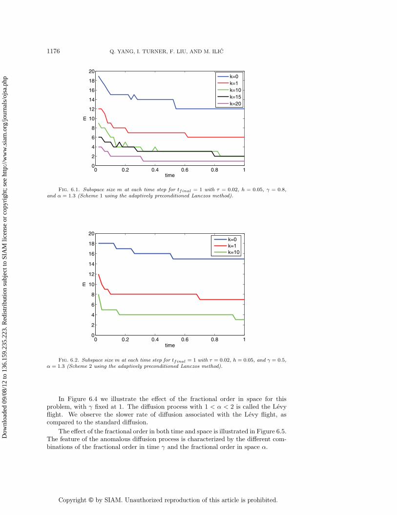
The performance of the preconditioner used in the Lanczos method is highlightedin Figures 6.1 and 6.2. Figure 6.1 is generated using Scheme 1 with the adaptivelypreconditioned Lanczos method for the test problem with tfinal = 1, τ = 0.02, h =0.05, γ = 0.8, α = 1.3. In this figure, we illustrate the impact of the preconditioner onthe size of the Krylov subspace m when k smallest approximate eigenpairs are used.This includes the case where k = 0, where no preconditioning was applied. We seethat the average subspace size m is reduced as we increase the number of eigenpairsfrom k = 1 to k = 20. In Figure 6.2, we see a similar impact of the preconditioner onthe subspace size m for the same test problem using Scheme 2. Another observationthat can be made from these figures is that as time evolves the size of the subspacem is reduced.
To further illustrate the effect of the fractional order in time and space, we presentanother example with the Delta function as the initial condition.
Example 2. Consider the TSFDE-2D (1.1)–(1.4) on the domain [0, 1]× [0, 1] withKα = 1 and u0(x, y) = δ(x− 1
2 , y− 12 ). In this example, we use Scheme 1 to compute
the numerical solution.In Figure 6.3 we illustrate the effect of the fractional order in time for this problem,
with α fixed at 2. The diffusion process with 0 < γ < 1 is called the subdiffusionprocess [26, 43, 17]. It is very interesting to see the appearance of cusps for thedifferent choices of fractional order in time γ, as compared to the standard diffusionwith γ = 1.
Fig. 6.1. Subspace size m at each time step for tfinal = 1 with τ = 0.02, h = 0.05, γ = 0.8,and α = 1.3 (Scheme 1 using the adaptively preconditioned Lanczos method).
0 0.2 0.4 0.6 0.8 10
2
4
6
8
10
12
14
16
18
20
time
m
k=0k=1k=10
Fig. 6.2. Subspace size m at each time step for tfinal = 1 with τ = 0.02, h = 0.05, and γ = 0.5,α = 1.3 (Scheme 2 using the adaptively preconditioned Lanczos method).
In Figure 6.4 we illustrate the effect of the fractional order in space for thisproblem, with γ fixed at 1. The diffusion process with 1 < α < 2 is called the Levyflight. We observe the slower rate of diffusion associated with the Levy flight, ascompared to the standard diffusion.
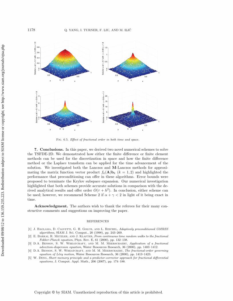
The effect of the fractional order in both time and space is illustrated in Figure 6.5.The feature of the anomalous diffusion process is characterized by the different com-binations of the fractional order in time γ and the fractional order in space α.
Fig. 6.5. Effect of fractional order in both time and space.
7. Conclusions. In this paper, we derived two novel numerical schemes to solvethe TSFDE-2D. We demonstrated how either the finite difference or finite elementmethods can be used for the discretization in space and how the finite differencemethod or the Laplace transform can be applied for the time advancement of thesolution. We investigated both the Lanczos and M-Lanczos methods for approxi-mating the matrix function vector product fk(A)bk (k = 1, 2) and highlighted theperformance that preconditioning can offer in these algorithms. Error bounds wereproposed to terminate the Krylov subspace expansion. Our numerical investigationhighlighted that both schemes provide accurate solutions in comparison with the de-rived analytical results and offer order O(τ + h2). In conclusion, either scheme canbe used; however, we recommend Scheme 2 if α + γ < 2 in light of it being exact intime.
Acknowledgment. The authors wish to thank the referees for their many con-structive comments and suggestions on improving the paper.
REFERENCES
[1] J. Baglama, D. Calvetti, G. H. Golub, and L. Reichel, Adaptively preconditioned GMRESalgorithms, SIAM J. Sci. Comput., 20 (1998), pp. 243–269.
[2] E. Barkai, R. Metzler, and J. Klafter, From continuous time random walks to the fractionalFokker-Planck equation, Phys. Rev. E, 61 (2000), pp. 132–138.
[3] D.A. Benson, S. W. Wheatcraft, and M. M. Meerschaert, Application of a fractionaladvection-dispersion equation, Water Resources Research, 36 (2000), pp. 1403–1412.
[4] D.A. Benson, S. W. Wheatcraft, and M. M. Meerschaert, The fractional-order governingequation of Levy motion, Water Resources Research, 36 (2000), pp. 1413–1423.
[5] W. Deng, Short memory principle and a predictor-corrector approach for fractional differentialequations, J. Comput. Appl. Math., 206 (2007), pp. 174–188.
[6] K. Diethelm, J. M. Ford, N. J. Ford, and M. Weilbeer, Pitfalls in fast numerical solversfor fractional differential equations, J. Comput. Appl. Math., 186 (2006), pp. 482–503.
[7] V. Druskin and L. Knizhnerman, Krylov subspace approximations of eigenpairs and matrixfunctions in exact and computer arithmetic, Numer. Linear Algebra Appl., 2 (1995), pp. 205–217.
[8] M. Eiermann and O. G. Ernst, A restarted Krylov subspace method for the evaluation ofmatrix functions, SIAM J. Numer. Anal., 44 (2006), pp. 2481–2504.
[9] H. C. Elman, D. J. Silvester, and A. J. Wathen, Finite Elements and Fast Iterative Solvers,Oxford University Press, Oxford, UK, 2005.
[10] A. Erdelyi, ed., Tables of Integral Transforms, McGraw–Hill, New York, 1954.[11] J. Erhel, K. Burrage, and B. Pohl, Restarted GMRES preconditioned by deflation, J. Com-
put. Appl. Math., 69 (1996), pp. 303–318.[12] A. Essai, Weighted FOM and GMRES for solving nonsymmetric linear systems, Numer. Algo-
rithms, 18 (1998), pp. 277–292.[13] N. J. Ford and A. C. Simpson, The numerical solution of fractional differential equations:
Speed versus accuracy, Numer. Algorithms, 26 (2001), pp. 333–346.[14] R. Gorenflo, F. Mainardi, E. Scalas, and M. Raberto, Fractional calculus and
continuous-time finance. III. The diffusion limit, in Mathematical Finance (Konstanz, 2000),Birkhauser, Basel, 2001, pp. 171–180.
[15] R. Gorenflo, J. Loutchko, and Y. Luchko, Computation of the Mittag-Leffler function Eα,β
and its derivative, Fract. Calc. Appl. Anal., 5 (2002), pp. 491–518.[16] M. G. Hall and T. R. Barrick, From diffusion-weighted MRI to anomalous diffusion imaging,
Magnetic Resonance in Medicine, 59 (2008), pp. 447–455.[17] B. I. Henry, T. A. M. Langlands, and S. L. Wearne, Fractional cable models for spiny
neuronal dendrites, Phys. Rev. Lett., 100 (2008), 128103.[18] R. Hilfer, Applications of Fractional Calculus in Physics, World Scientific, Singapore, 2000.[19] R. Hilfer, Threefold introduction to fractional derivatives, in Anomalous Transport: Foun-
dations and Applications, R. Klages, G. Radons, and I. M. Sokolov, eds., Wiley-VCH,Weinheim, Germany, 2008, pp. 17–74.
[20] M. Hochbruck and C. Lubich, On Krylov subspace approximations to the matrix exponentialoperator, SIAM J. Numer. Anal., 34 (1997), pp. 1911–1925.
[21] M. Ilic, F. Liu, I. Turner, and V. Anh, Numerical approximation of a fractional-in-spacediffusion equation I, Fract. Calc. Appl. Anal., 8 (2005), pp. 323–341.
[22] M. Ilic, F. Liu, I. Turner, and V. Anh, Numerical approximation of a fractional-in-spacediffusion equation II. With nonhomogeneous boundary conditions, Fract. Calc. Appl. Anal.,9 (2006), pp. 333–349.
[23] M. Ilic, I. Turner, and V. Anh, A numerical solution using an adaptively preconditionedLanczos method for a class of linear systems related with the fractional Poisson equation,J. Appl. Math. Stoch. Anal., (2008), 104525.
[24] M. Ilic, I. W. Turner, and D. P. Simpson, A restarted Lanczos approximation to functionsof a symmetric matrix, IMA J. Numer. Anal., 30 (2010), pp. 1044–1061.
[25] Y. W. Kwon and H. Bang, The Finite Element Method Using MATLAB, CRC Press LLC,Boca Raton, FL, 2000.
[26] T. A. M. Langlands and B. I. Henry, The accuracy and stability of an implicit solutionmethod for the fractional diffusion equation, J. Comput. Phys., 205 (2005), pp. 719–736.
[27] R. B. Lehoucq and D. C. Sorensen, Deflation techniques for an implicitly restarted Arnoldiiteration, SIAM J. Matrix Anal. Appl., 17 (1996), pp. 789–821.
[28] Y. Lin and C. Xu, Finite difference/spectral approximations for the time-fractional diffusionequation, J. Comput. Phys., 225 (2007), pp. 1533–1552.
[29] F. Liu, V. Anh, and I. Turner, Numerical solution of the space fractional Fokker-Planckequation, J. Comput. Appl. Math., 166 (2004), pp. 209–219.
[30] F. Liu, I. Turner, and V. Anh, An unstructured mesh finite volume method for modellingsaltwater intrusion into coastal aquifers, Korean J. Comput. Appl. Math., 9 (2002), pp. 391–407.
[31] L. Lopez and V. Simoncini, Analysis of projection methods for rational function approximationto the matrix exponential, SIAM J. Numer. Anal., 44 (2006), pp. 613–635.
[32] R. Magin, X. Feng, and D. Baleanu, Solving the fractional order Bloch equation, Conceptsin Magnetic Resonance Part A, 34A (2009), pp. 16–23.
[33] M. Matsuki and T. Ushijima, A note on the fractional powers of operators approximatinga positive define selfadjoint operator, J. Fac. Sci. Univ. Tokyo Sect. IA Math., 40 (1993),pp. 517–528.D
[34] M. M. Meerschaert and E. Scalas, Coupled continuous time random walks in finance,Phys. A, 370 (2006), pp. 114–118.
[35] R. Metzler and J. Klafter, Boundary value problems for fractional diffusion equations,Phys. A, 278 (2000), pp. 107–125.
[36] R. Metzler and J. Klafter, The random walk’s guide to anomalous diffusion: A fractionaldynamics approach, Phys. Rep., 339 (2000), pp. 1–77.
[37] I. Podlubny, Fractional Differential Equations, Academic Press, New York, 1999.[38] M. Raberto, E. Scalas, and F. Mainardi, Waiting-times and returns in high-frequency fi-
nancial data: An empirical study, Phys. A, 314 (2002), pp. 749–755.[39] Y. Saad, Analysis of some Krylov subspace approximations to the matrix exponential operator,
SIAM J. Numer. Anal., 29 (1992), pp. 209–228.[40] Y. Saad, Iterative Methods for Sparse Linear Systems, PWS, Boston, MA, 1993.[41] A. I. Saichev and G. M. Zaslavsky, Fractional kinetic equations: Solutions and applications,
Chaos, 7 (1997), pp. 753–764.[42] S. G. Samko, A. A. Kilbas, and O. I. Marichev, Fractional Integrals and Derivatives: Theory
and Applications, Gordon and Breach Science Publishers, Amsterdam, 1993.[43] M. Saxton, Anomalous subdiffusion in fluorescence photobleaching recovery: A Monte Carlo
study, Biophys. J., 81 (2001), pp. 2226–2240.[44] E. Scalas, R. Gorenflo, and F. Mainardi, Fractional calculus and continuous-time finance,
Phys. A, 284 (2000), pp. 376–384.[45] R. B. Sidje, Expokit: A software package for computing matrix exponentials, ACM Trans.
Math. Softw., 24 (1998), pp. 130–156.[46] V. Simoncini and D. B. Szyld, Recent computational developments in Krylov subspace methods
for linear systems, Numer. Linear Algebra Appl., 14 (2007), pp. 1–59.[47] D. Simpson, Krylov Subspace Methods for Approximating Functions of Symmetric Positive
Definite Matrices with Applications to Applied Statistics and Anomalous Diffusion, Ph.D.Thesis, Queensland University of Technology, Brisbane, Australia, 2009.
[48] I. Turner, M. Ilic, and P. Perre, The use of fractional-in-space diffusion equations fordescribing microscale diffusion in porous media, in the Proceedings of the 17th InternationalDrying Symposium (IDS 2010), Magdeburg, Germany, 2010, pp. 432–437.
[49] J. van den Eshof, A. Frommer, T. Lippert, K. Schilling, and H. van der Vorst, Numericalmethods for the QCD overlap operator. I. Sign-function and error bounds, Comput. Phys.Commun., 146 (2002), pp. 203–224.
[50] H. A. van der Vorst, An iterative solution method for solving f(A)x = b using Krylov subspaceinformation obtained for the symmetric positive definite matrix A, J. Comput. Appl. Math.,18 (1987), pp. 249–263.
[51] W. Wyss, The fractional Black-Scholes equation, Fract. Calc. Appl. Anal., 3 (2000), pp. 51–61.[52] Q. Yang, Novel Analytical and Numerical Methods for Solving Fractional Dynamical Systems,
Ph.D. thesis, Queensland University of Technology, Brisbane, Australia, 2010.[53] Q. Yang, F. Liu, and I. Turner, Numerical methods for fractional partial differential equations
with Riesz space fractional derivatives, Appl. Math. Model., 34 (2010), pp. 200–218.[54] S. B. Yuste, L. Acedo, and K. Lindenberg, Reaction front in an A + B –> C reaction-
subdiffusion process, Phys. Rev. E, 69 (2004), 036126.[55] S. B. Yuste and K. Lindenberg, Subdiffusion-limited A + A reactions, Phys. Rev. Lett., 87
(2001), 118301.[56] G. M. Zaslavsky, Chaos, fractional kinetics, and anomalous transport, Phys. Rep., 371 (2002),