NOVEL PACKAGING DESIGNS FOR IMPROVEMENTS IN AIR …

NOVEL PACKAGING DESIGNS FOR IMPROVEMENTS

IN AIR FILTER PERFORMANCE

Except where reference is made to the work of others, the work described in this dissertation is my own or was done in collaboration with my advisory committee.

This dissertation does not include proprietary or classified information.

_____________________________________ Ryan Anthony Sothen

Certificate of Approval: W. Robert Ashurst Bruce J. Tatarchuk, Chair Assistant Professor Professor Chemical Engineering Chemical Engineering Mario R. Eden Daniel Harris Associate Professor Associate Professor Chemical Engineering Mechanical Engineering

George T. Flowers Dean Graduate School

ii


IN AIR FILTRATION PERFORMANCE

Ryan Anthony Sothen

A Dissertation

Submitted to

the Graduate Faculty of

Auburn University

in Partial Fulfillment of the

Requirements for the

Degree of

Doctor of Philosophy

Auburn, Alabama

August 10th, 2009

iii



Ryan Anthony Sothen

Permission is granted to Auburn University to make copies of this dissertation at its discretion, upon request of individuals or institutions and at their expense.

The author reserves all publication rights.

______________________________ Signature of Author ______________________________ Date of Graduation

iv

VITA

Ryan A. Sothen was born and raised by James E. and Lois R. Sothen in

Charleston, West Virginia. He began his collegiate studies in the Department of

Chemical Engineering at Virginia Polytechnic Institute & State University (Virginia

Tech). During his time at Virginia Tech, he worked outside the classroom as an

analytical chemist for Dominion Semiconductor and performed undergraduate research

on polymeric materials for Dr. Donald Baird. Ryan completed his Bachelor of Science in

the Spring of 2004, and subsequently enrolled in the Chemical Engineering Graduate

Program at Auburn University during the Fall of 2004.

v

DISSERTATION ABSTRACT



Ryan Anthony Sothen

Doctor of Philosophy, August 10, 2009 (B.S., Virginia Polytechnic Institute & State University, 2004)

234 Typed Pages

Directed by Bruce J. Tatarchuk

Adsorbent entrapped media, such as microfibrous materials engineered at Auburn

University, provide a novel method to effectively remove harmful airborne contaminants

such as volatile organic compounds and particulate matter from polluted indoor air.

These dual-functioning materials are limited in their use as air filters due to their high

pressure drops and relatively small loading of adsorbent material. Utilization of a pleated

filter design is a common approach in the air filtration industrial to increase the available

media and reduce the pressure drop of a media. A second technique was developed to

greatly increase the capacity and further reduce the pressure drop by employing

numerous pleated filters into a single filter unit known as a Multi-Element Structured

Array (MESA).

vi

A comprehensive pressure drop model was constructed to understand the working

parameter space within these filter designs. The model was formulated on fundamental

fluid dynamics equations such as Bernoulli’s Equation and empirical data obtained on

custom-made filter units. The working models were shown to be successful in replicating

over 1500 data points spanning 20 pleated filters and 32 MESA units.

Several niche filtration designs were envisioned during the development of the

model. These designs were subsequently tested to demonstrate their performance

advantage over standard HVAC pleated designs based on dirt holding and power

consumption. It was determined that MESA architectures can be utilized to provided

equal or superior particulate removal efficiency while operating at only 20% of the power

of a traditional pleated filter.

vii

ACKNOWLEDGMENTS

The author would like to express his sincere gratitude to Dr. Bruce J. Tatarchuk for

his guidance throughout the course of my graduate studies. I would like to acknowledge the

US Army (TARDEC) for funding the research presented in this dissertation. I would also like

to thank my committee members Dr. Mario Eden, Dr. W. Robert Ashurst, Dr. Daniel Harris,

and Dr. Christopher Roy for their time and efforts to ensure the compilation of this work.

Special thanks are in order for all of my past and present CM3 colleagues. In

particular, I would like to acknowledge the members of the filtration group. My upmost

appreciations are in order to Mr. Ron Putt and Mr. Amogh Karwa for their assistance in

helping me with laboratory and theoretical issues as well as Mrs. Yanli “Joyce” Chen for her

assistance with laboratory experimentation over the last six months. I would like to thank the

following members of the Faculty and Staff who have helped me greatly during my time at

Auburn: Mrs. Sue Ellen Abner, Mr. Dwight Cahela, Mrs. Karen Cochran, Mrs. Jennifer

Harris, Dr. Lewis Payton, Dr. Christopher Roberts, Mrs. Megan Schumacher, and Mr. Brian

Scweiker. Lastly, I would like to thank Dr. Donald Baird and Dr. Y. A. Liu for supporting

and encouraging me to continue my education career after complication of my Bachelor of

Science at Virginia Tech.

viii

Style manual or journal used: HVAC & R Research Computer software used: Microsoft Word

ix

TABLE OF CONTENTS

LIST OF FIGURES ......................................................................................................... xiii

LIST OF TABLES.......................................................................................................... xxii

Chapter I: Introduction to Air Filtration ..............................................................................1

I.1 Motivation ..........................................................................................................1

I.2. Microfibrous Media...........................................................................................3

I.3. Influence of Pressure Drop within a HVAC System.........................................5

Chapter II: Background & Experimental for Modeling Initial Pressure Drop ....................8

II.1. Previous Pleated Filter Models ........................................................................8

II.1.1. Chen et al...........................................................................................8

II.1.2. Rivers & Murphy ............................................................................10

II.1.3. Del Fabbro et al ...............................................................................10

II.1.4. Caeser and Schroth..........................................................................11

II.1.5. Tronville and Sala ...........................................................................12

II.1.6. Raber ...............................................................................................13

II.2. Objectives of Current Modeling Efforts.........................................................14

II.3 Theory .............................................................................................................15

II.3.1. Forchheimer-extended Darcy’s Law...............................................16

II.3.2. Mechanical Energy Balance / Bernoulli’s Equation .......................17

II.3.3. Equation of Continuity....................................................................21

II.3.4. Momentum Balance ........................................................................22

x

II.4. Experimental Setups.......................................................................................22

II.4.1. Media Test Rig................................................................................22

II.4.2. Filtration Test Rig ...........................................................................24

II.5. Data Acquisition.............................................................................................30

II.5.1. Media Pressure Drop Curves...........................................................30

II.5.2. Filter Pressure Drop Curves ............................................................30

II.5.3. Media Thickness .............................................................................34

Chapter III: Initial Pressure Drop Modeling of Pleated Filters..........................................35

III.1 Introduction....................................................................................................35

III.1.1. Pleated Filter Schematics...............................................................35

III.1.2. Parameters......................................................................................38

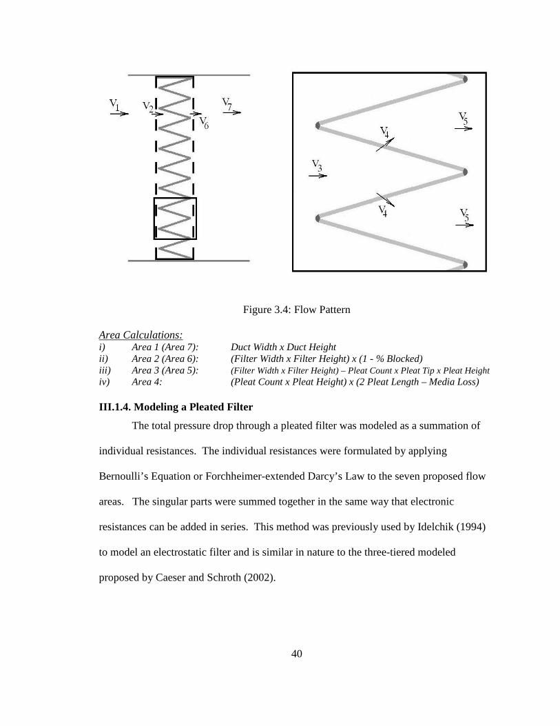
III.1.3 Proposed Flow through a Pleated Filter......................................................39

III.1.4 Modeling a Pleated Filter............................................................................40

III. 2. Identifying the Constants .............................................................................43

III. 2.1. Media Constants & Thickness ......................................................43

III. 2.2. Grating Coefficient of Friction (KG).............................................46

III. 2.3. Pleat Tip Assumption....................................................................50

III. 2.4. Pleat Coefficient of Friction (KP) .................................................51

III. 2.5. Reevaluate the Pleat Tip Contraction and Expansion...................58

III.3. Utilization and Discussion of the Model ......................................................60

III. 3.1. Pleating Curve...............................................................................60

III. 3.2. Location of the Optimal Pleat Count ............................................63

III. 3.3. Influence of Design Parameters ....................................................64

xi

III. 3.4. Limitations of the Model ..............................................................77

Chapter IV. Initial Pressure Drop of Multi-Element Structured Arrays............................78

IV.1. Introduction...................................................................................................78

IV.1.1. Multi-Element Structured Arrays Schematic.................................78

IV.1.2. Parameters......................................................................................80

IV.1. 3. Proposed Flow through a MESA..................................................82

IV.1. 4. Modeling a Multi-Element Structured Arrays..............................84

IV.2. Multi-Filter Bank Experimental ...................................................................85

IV.2. 1. Entrance Coefficient of Friction (KCB) .........................................86

IV.2. 2. Exit Coefficient of Friction (KEB).................................................89

IV.2.3. Slot Coefficient of Friction (KS)....................................................91

IV.3. Discussion Utilizing the Model ....................................................................98

IV.3.1. Achievement of Objectives............................................................98

IV.3.2. The Pleating Curve of a MESA.....................................................99

IV.3.3. Locating the Optimal Pleat Count ...........................................................102

IV.3.4. Influence of Design Parameters...............................................................102

Chapter V: Theory & Experimental for Air Filtration Performance ...............................117

V.1. Introduction..................................................................................................117

V.2. Theory ..........................................................................................................117

V.2.1. Previous Research concerning Dirt Loading of Air Filters...........117

V.2.2. Particulate Removal Efficiency by Fibrous Media .......................119

V.3. Experimental ................................................................................................122

V.3.1. Test Rig and Equipment................................................................122

xii

V.3.2. Experimental Data Acquisition.....................................................130

V.3.2.1. Volumetric Flow ............................................................130

V.3.2.2. Pressure Drop across Filtration Section .........................134

V.3.2.3. Particle Count.................................................................134

V.3.3. Testing Procedures........................................................................136

V.3.3.1. Initial Pressure Drop ......................................................136

V.3.3.2 Testing Procedure for Dirt Loading ................................138

V.3.3.3. Removal Efficiency Testing..........................................141

Chapter VI: Filtration Performance of Novel, Single Element Designs..........................143

VI.1. Introduction.................................................................................................143

VI.2. Materials and Methods ...............................................................................143

VI.3. Results and Discussion ...............................................................................144

VI.3.1. Initial Resistance..........................................................................144

VI.3.2. Dirt Loading.................................................................................147

VI.3.3. Estimations of Useful Lifetime and Power Consumption ...........160

Chapter VII: Filtration performance of Multi-Element Structured Arrays......................165

VII.1. Introduction ...............................................................................................165

VII.2. Particulate Removal Efficiency of a MEPFB............................................165

VII.2.1. Materials.....................................................................................166

VII.2.2. Results and Discussion...............................................................166

VII.3. Dirt Loading of MESA’s...........................................................................170

VII.3.1. Materials.....................................................................................170


xiii

VII.3.2.1. Influence of Pleat Count within an MESA..................170

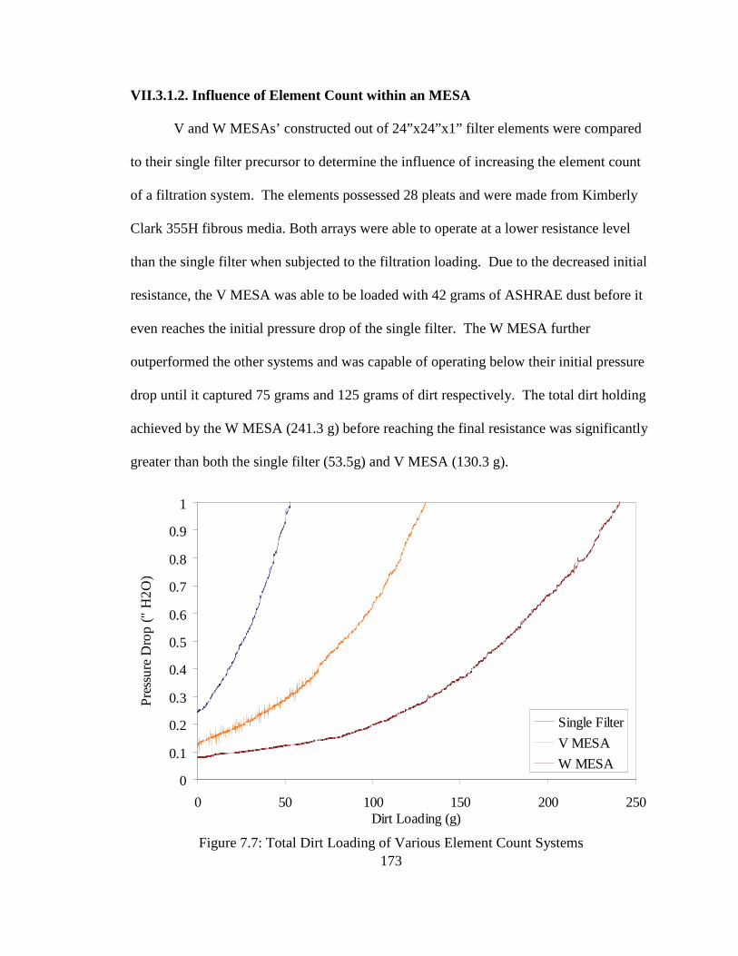
VII.3.2.2. Influence of Element Count ........................................173

VII.3.2.3. Power Consumption Analysis .....................................176

VII.4. Preferential Element Alignment within a MESA......................................177

VII.4.1. Materials and Methods ...............................................................177


VII.4.2.1. Initial Pressure Drop....................................................179

VII.4.2.2. Dirt Loading ................................................................181

Chapter VIII: Conclusions and Future Work...................................................................192

VIII.1. Conclusions..............................................................................................192

VIII.2. Future Work .............................................................................................193

V.III.1. Utilization of Fairings .................................................................194

V.III.2. Media Compression versus Permeability....................................194

V.III.3 Pyramid Filter ..............................................................................195

References........................................................................................................................196

Appendix A......................................................................................................................197

A.1 Rotameter Calibration...................................................................................199

A.2 Calibration of Pressure Transducers .............................................................202

A.3 Construction of Filter Holder........................................................................204

A.4 Construction of MESA Unit .........................................................................204

A.5 Weight Increase of ASHRAE Dust under Atmospheric Conditions ............206

A.6 Observed Flow Channeling due to Pleat Tip Blockage ................................207

A.7 Determination of Ramping Rate ...................................................................208

xiv

Appendix B: Nomenclature .............................................................................................211

B.1 Arabic Symbols .............................................................................................211

B.2 Greek Symbols ..............................................................................................212

B.3. Subscripts .....................................................................................................212

xv

LIST OF FIGURES

Figure 1.1: Typical “U” Pleating Curve ..............................................................................7

Figure 2.1: Sudden Contraction Diagram ..........................................................................19

Figure 2.2: Sudden Expansion Diagram ............................................................................19

Figure 2.3: Gradually Contraction Diagram ......................................................................20

Figure 2.4: Grating Diagram..............................................................................................20

Figure 2.5: Duct Diagrams.................................................................................................21

Figure 2.6: General Schematic of Media Test Rig ............................................................23

Figure 2.7: Control Pressure Drop Curve for Media Test Rig...........................................24

Figure 2.8: General Schematic of Blower Test Rig...........................................................25

Figure 2.9: Flow Distribution at 40 Hz Before (A) and After (B).....................................26

Figure 2.10: Coefficient of Variance .................................................................................28

Figure 2.11: Control Pressure Drop Curve for Filter Test Rig ..........................................29

Figure 2.12: Measurement Path for the Vane Anemometer .............................................31

Figure 2.13: Velocity Measurement Comparison..............................................................33

Figure 2.14: Pressure Measurement Comparison ..............................................................34

Figure 3.1: Pleated Filter Illustration .................................................................................36

Figure 3.2: Illustration of Pleat Dimensions......................................................................37

Figure 3.3: Pleat Tip Illustration........................................................................................38

Figure 3.4: Flow Pattern ....................................................................................................40

xvi

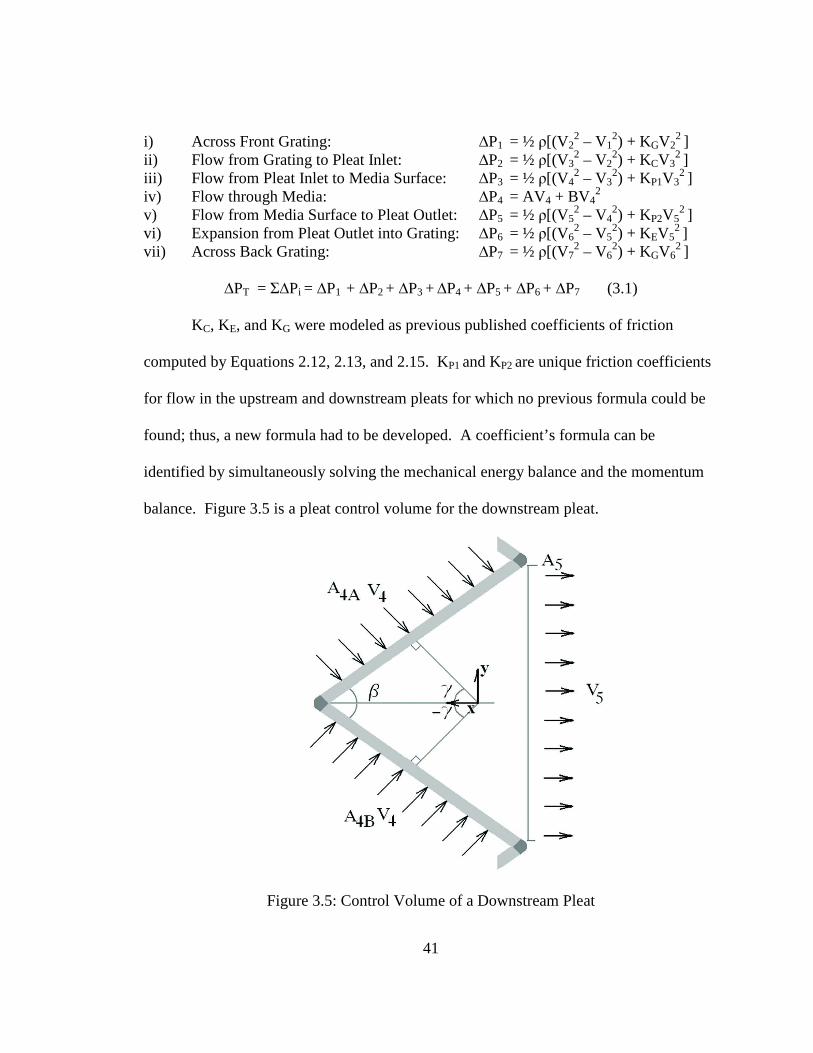
Figure 3.5: Control Volume of a Downstream Pleat .........................................................41

Figure 3.6: Media Resistance Curves ................................................................................44

Figure 3.7: Darcy’s Law Analysis of Media Resistance....................................................46

Figure 3.8: Illustration of Grating Schemes.......................................................................47

Figure 3.9: Pressure Drop Curves for Various Frontal Blockages ....................................47

Figure 3.10: Computed Grating Resistances .....................................................................48

Figure 3.11: Effects of Front Grating Modification...........................................................49

Figure 3.12: Effects of Back Grating Modification ...........................................................50

Figure 3.13: Pressure Drop Curves for a 20”x20”x1” FM1 Filter with 42 Pleats .............52

Figure 3.14: Pleat Coefficient Graph for a 20”x20”x1” FM1 Filter with 42 Pleats ..........53

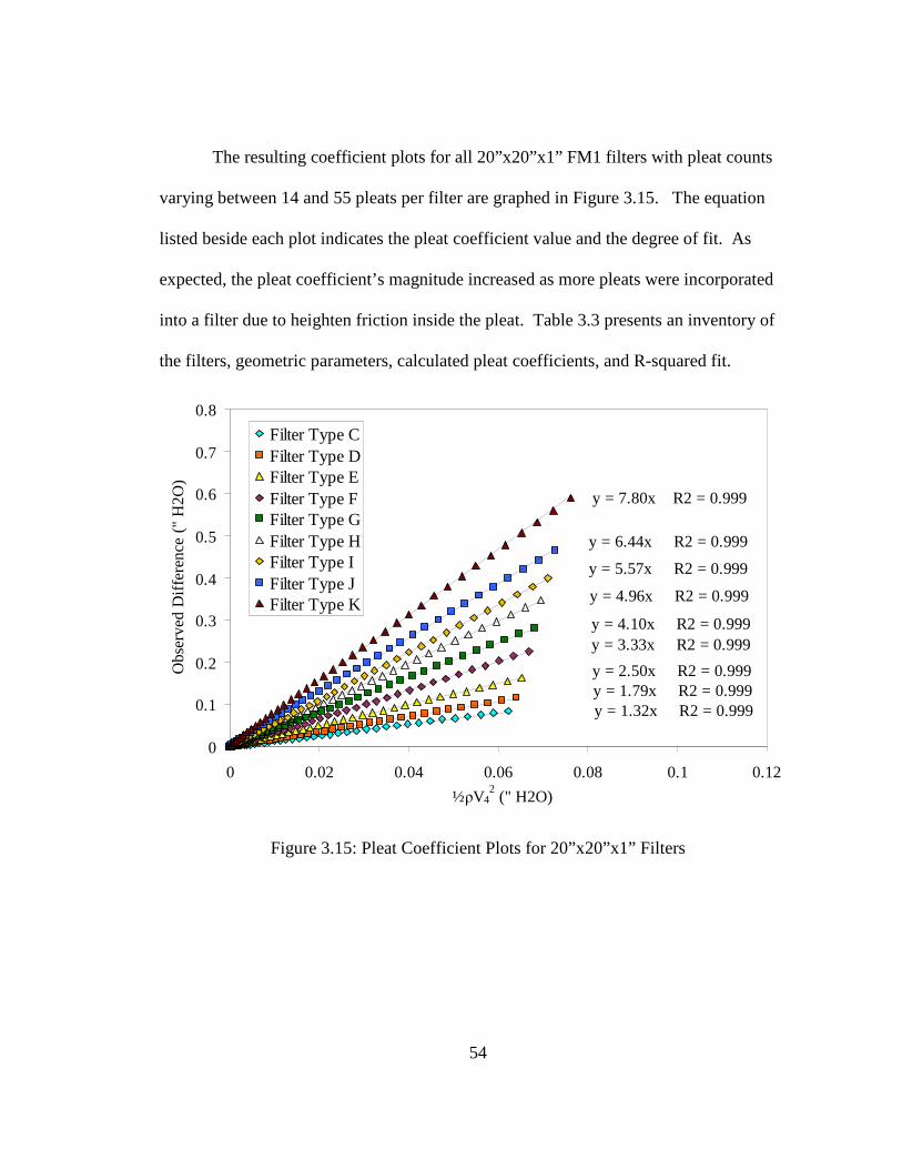
Figure 3.15: Pleat Coefficient Plots for 20”x20”x1” Filters..............................................54

Figure 3.16: Pleat Coefficient Graph .................................................................................56

Figure 3.17: A Linear Pleat Coefficient Plot .....................................................................57

Figure 3.18: Correlation Plot between Empirical and Modeled Pleat Coefficients...........58

Figure 3.19: Modified Correlation Plot .............................................................................59

Figure 3.20: Pleating Curve and Individual Resistances ...................................................61

Figure 3.21: Optimal Pleat Count Location.......................................................................64

Figure 3.22: Effects of Face Velocity on Pleating Curve ..................................................67

Figure 3.23: Effects of Media Thickness on Pleating Curve .............................................68

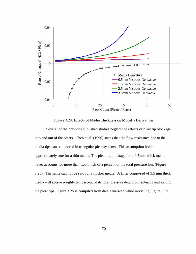
Figure 3.24: Effects of Media Thickness on Model’s Derivatives ....................................70

Figure 3.25: Modeled Pleat Tip Contribution to Total Resistance 20”x20”x1” Filters.....71

Figure 3.26: Modeled Effects of Filter Depth on Pleating Curve......................................72

Figure 3.27: Effects of Filter Depth on Model Derivatives ...............................................73

xvii

Figure 3.28: Effects of Filter Depth on Performance Curve..............................................74

Figure 3.29: Effects of Media Resistance on Pleating Curve ............................................75

Figure 3.30: Effects of Media Resistance on Model’s Derivatives ...................................76

Figure 4.1: General Schematic of a Multi-Element Structured Array...............................79

Figure 4.2: Array Configurations (A) “W” (B) “WV” Configuration (C) “WW” ............80

Figure 4.3: General Diagram of Multi-Filter Array...........................................................82

Figure 4.4: Proposed Flow Profile .....................................................................................83

Figure 4.5: Illustration and Schematic of Flow within a Normal (A) and Contraction Modified Array (B) ..............................................................87

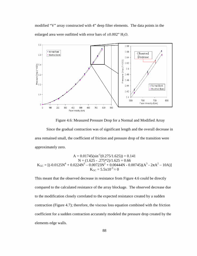
Figure 4.6: Measured Pressure Drop for a Normal and Modified Array...........................88

Figure 4.7: Observed and Modeled Pressure Drop Differences ........................................89

Figure 4.8: Illustration and Schematic of Flow within a Normal (A) and Expansion Modified Array (B) ..........................................................................................90

Figure 4.9: Measured Pressure Drop for a Normal and Modified Array...........................90

Figure 4.10: Observed and Modeled Pressure Drop Differences ......................................91

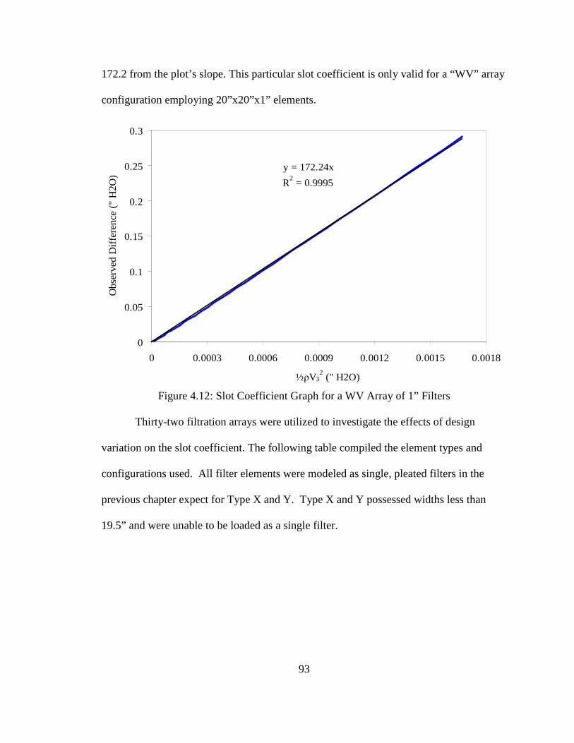
Figure 4.11: Pressure Drop Curves for a WV Array of 1” Filters .....................................92

Figure 4.12: Slot Coefficient Graph for a WV Array of 1” Filters....................................93

Figure 4.13: Slot Coefficient Plots for Various Configurations ........................................95

Figure 4.14: Slot Coefficient Graph...................................................................................97

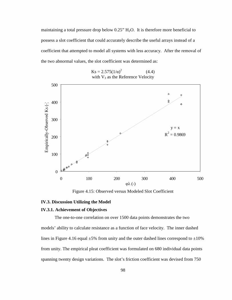
Figure 4.15: Observed versus Modeled Slot Coefficient...................................................98

Figure 4.16: Correlation Plot between Observed and Modeled Data ................................99

Figure 4.17: Multi-element structured array Pleating Curve ...........................................100

Figure 4.18: Percentage Contribution of (A) Single Filter and (B) “W” Array ..............101

Figure 4.19: Effects of Element Count on MESA Pleating Curve ..................................104

xviii

Figure 4.20: Effect of Element Count on Contribution of the pressure drop ..................105

Figure 4.21: Effects of Element Count on MESA Performance Curve...........................106

Figure 4.22: Effects of Element Width on MESA Performance Curve...........................108

Figure 4.23: Effect of Element Width on Contribution ...................................................109

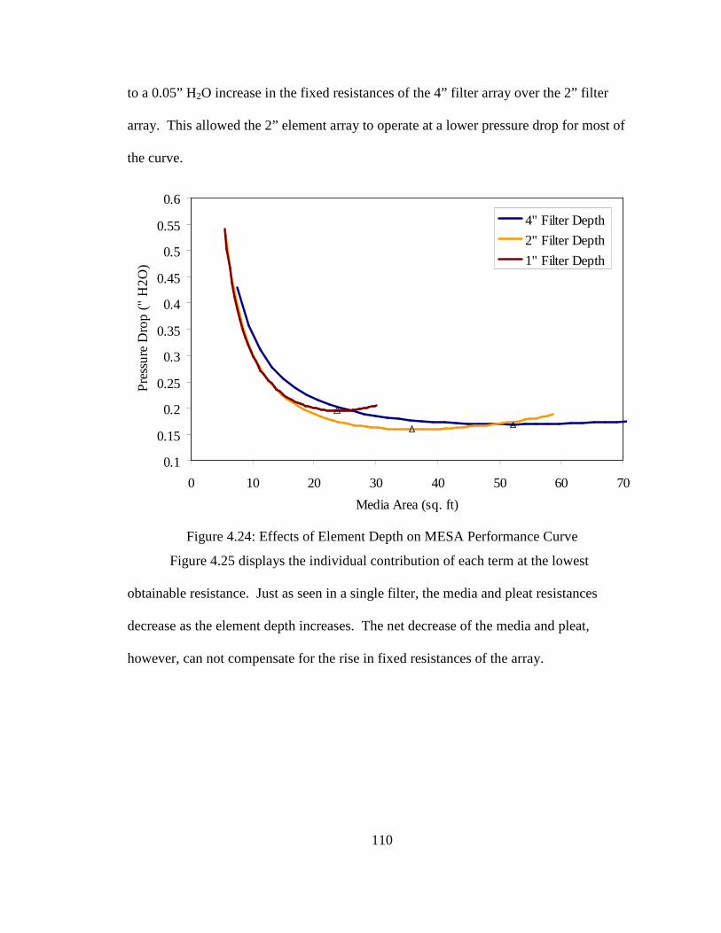
Figure 4.24: Effects of Element Depth on MESA Performance Curve...........................110

Figure 4.25: Effect of Element Depth on Contribution ...................................................111

Figure 4.26: Effects of Media Constants on MESA Pleating Curve ...............................112

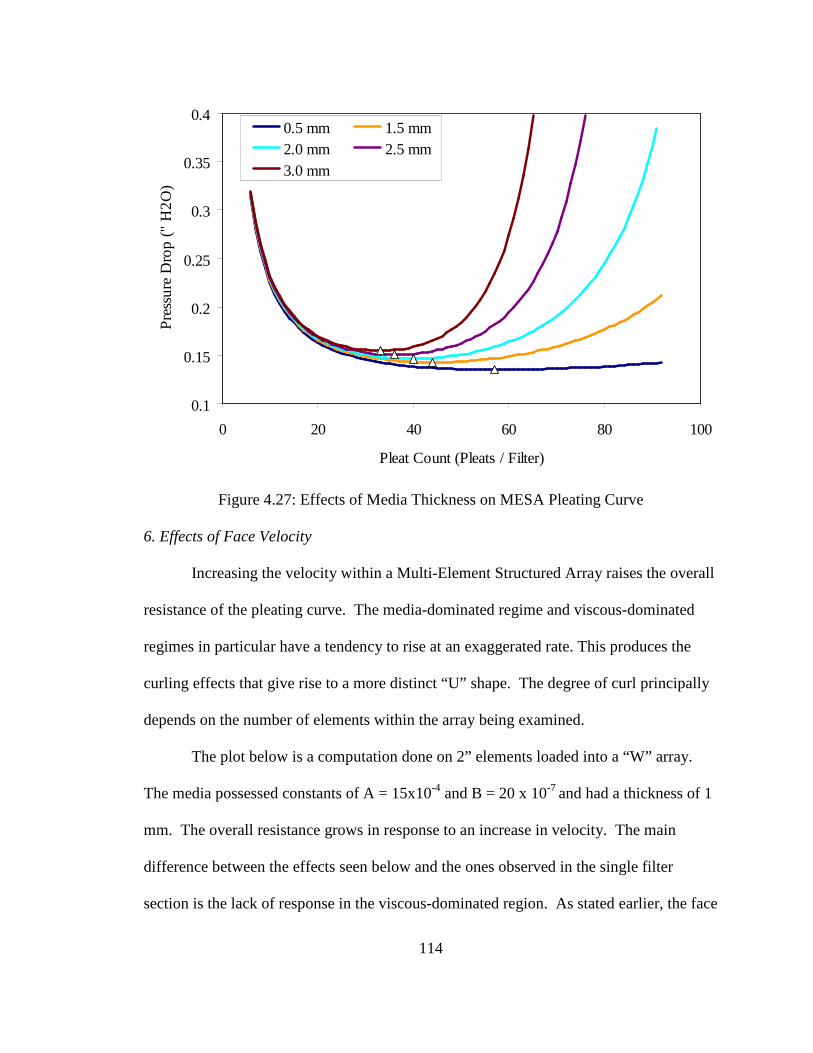
Figure 4.27: Effects of Media Thickness on MESA Pleating Curve...............................114

Figure 4.28: Effects of Velocity on MESA Pleating Curve.............................................115

Figure 5.1: General Trend in Filter Loading....................................................................119

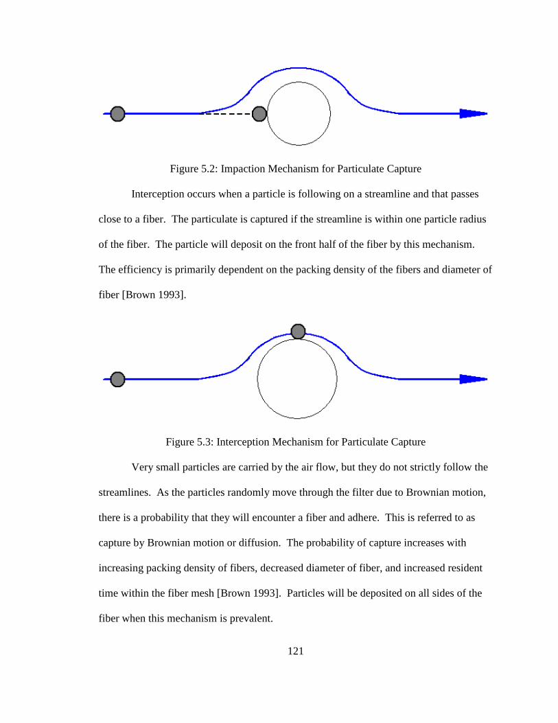
Figure 5.2: Impaction Mechanism for Particulate Capture..............................................121

Figure 5.3: interception Mechanism for Particulate Capture...........................................121

Figure 5.4: Particulate Capture by Brownian Motion......................................................122

Figure 5.5: Schematic of Full Scale Test Rig ..................................................................123

Figure 5.6: upstream Picture of the Test Rig ...................................................................123

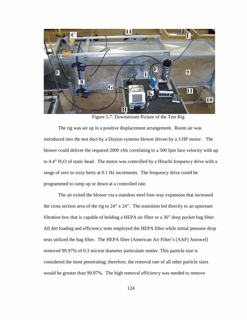
Figure 5.7: Downstream Picture of the Test Rig .............................................................124

Figure 5.8: Removal Efficiency of Upstream Filters.......................................................125

Figure 5.9: TSI 8108 Large Particle Generator Schematic..............................................128

Figure 5.10: Schematic and Picture of Sealing System ...................................................130

Figure 5.11: Blower and Tap Configuration....................................................................133

Figure 5.12 Face Velocity Calibration Curve for Test Rig’s Orifice Plate .....................134

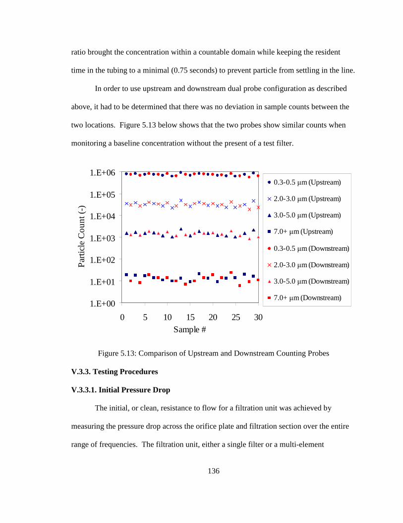
Figure 5.13: Comparison of Upstream and Downstream Counting Probes.....................136

Figure 5.14: Alignment and Clamping System................................................................137

xix

Figure 5.15: Loading Tray with leveling Tool.................................................................140

Figure 6.1: Pleating Curve for 24”x24”x1” Filters at 500 fpm: Filters composed of 411 SF media .............................................................................................145

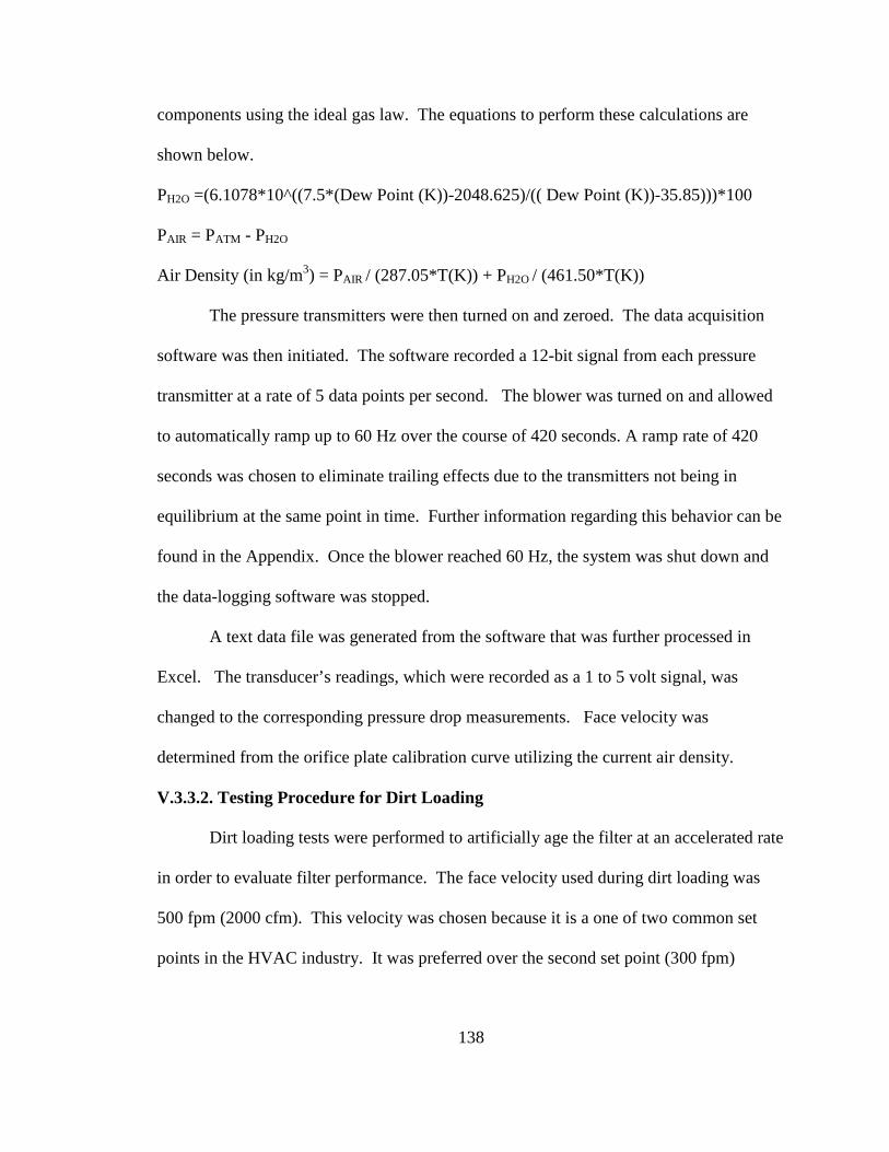
Figure 6.2: Pleating Curve for 24”x24”x2” Filters at 500 fpm: Filters composed of 411 SF media ............................................................................................146 Figure 6.3: Pleating Curve for 24”x24”x4” Filters at 500 fpm Filters composed of 411 SF media.............................................................................................146 Figure 6.4: Dirt Loading for 24”x24”x1” Filters .............................................................148

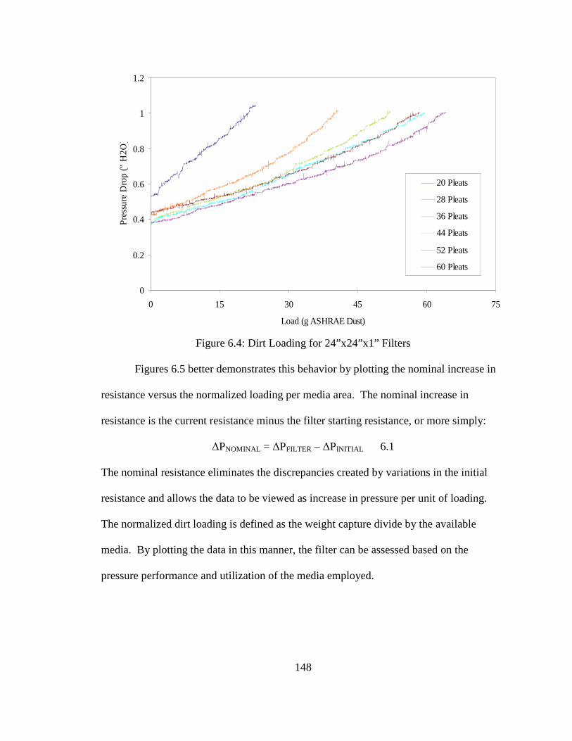
Figure 6.5: Normalized Loading Profiles of 24”x24”x1” Filters ...................................149

Figure 6.6: Depth Filtration Regime for 20 and 28 Pleat Filter......................................150

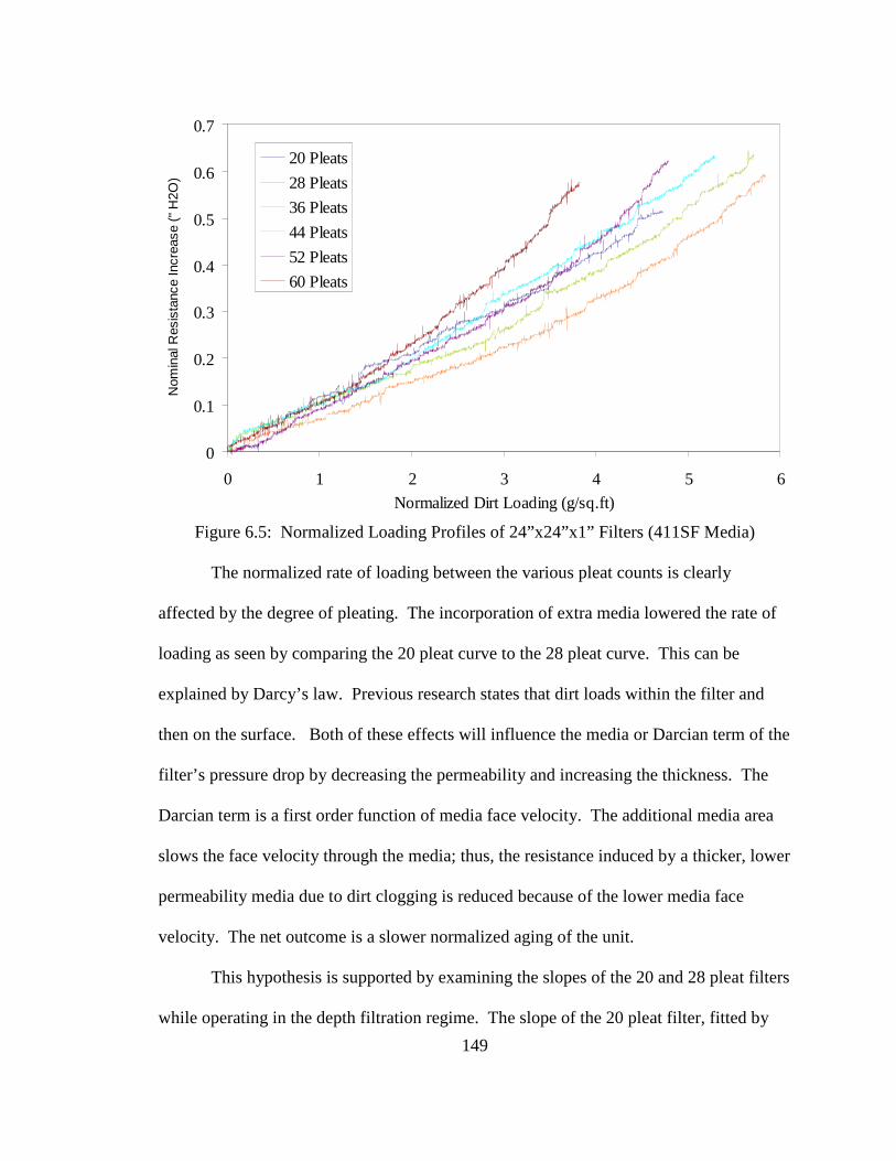
Figure 6.7: Schematic of Preferential Loading. (A) Low and (B) High Beta Angle.......151

Figure 6.8: Normalized Loading Profiles of Select 24”x24”x1” 411SF Filters with Transition Lines ....................................................................................152 Figure 6.9: Normalized Loading Profiles of 24”x24”x1” Filters composed

of 355H Filter Media ....................................................................................153

Figure 6.10: Dirt Loading for 24”x24”x2” Filters ...........................................................154

Figure 6.11: Normalized Dirt Loading for 24”x24”x2” Filters .......................................155

Figure 6.12: Dirt Loading for 24”x24”x4” Filters ...........................................................156

Figure 6.13: Normalized Dirt Loading for 24”x24”x2” Filters .......................................157

Figure 6.14: Relationship between Pleating Angle and Transition Point........................158

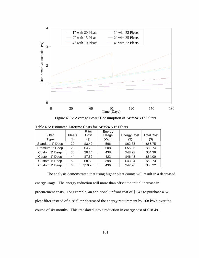
Figure 6.15: Average Power Consumption of 24”x24”x1” Filters..................................161



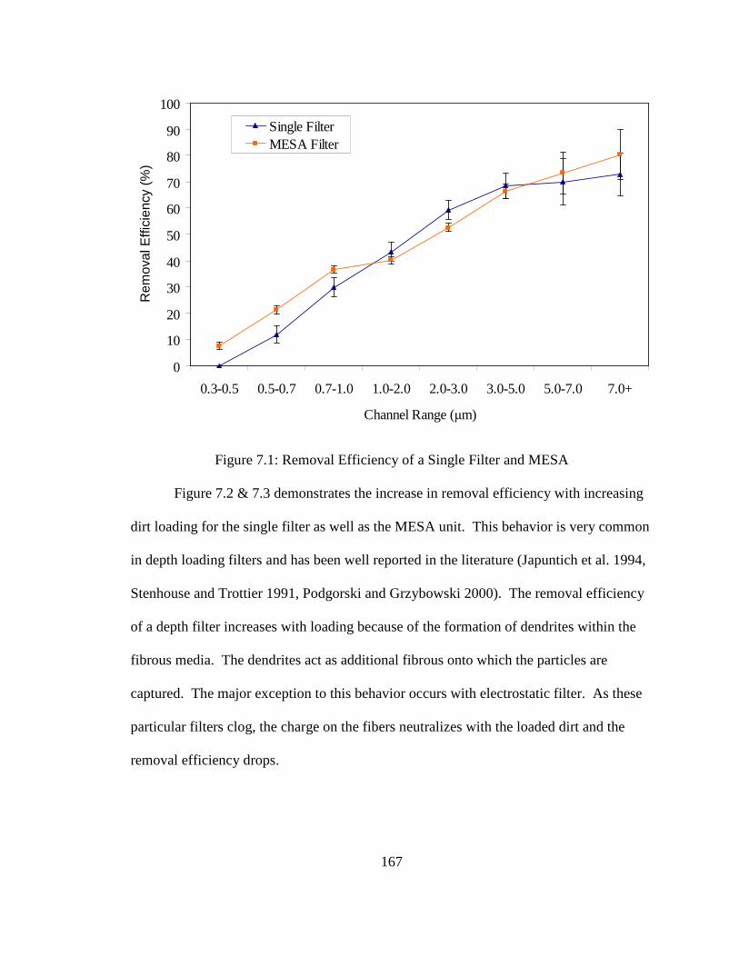
Figure 7.1: Removal Efficiency of a Single Filter and MESA........................................167

Figure 7.2: Removal Efficiency of a Single Element during Loading Conditions..........168

xx

Figure 7.3: Removal Efficiency of a MESA during Loading Conditions .......................168

Figure 7.4: Quality Factor Analysis.................................................................................169

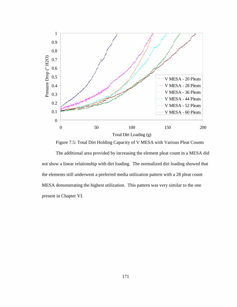
Figure 7.5: Total Dirt Holding Capacity of V MESA with Various Pleat Counts ..........171

Figure 7.6: Normalized Dirt Holding Capacity of V MESA with Various Pleat Counts ............................................................................................................172 Figure 7.7: Total Dirt Loading of Various Element Count Systems ...............................173

Figure 7.8: Normalized Loading Profile of a Various Element Count Systems with emphasis placed on the Depth Loading Regime............................................174 Figure 7.9: Normalized Loading Profile of a Various Element Count Systems with emphasis placed on the Cake Loading Regime .............................................176 Figure 7.10: Power Consumption of MESAs’ and Single Filter .....................................177

Figure 7.11: Horizontally-Oriented (Left) & Vertically-Oriented (Right) Banks ...........178

Figure 7.12: Clean Resistance of DP 4-40 Elements Loaded Vertically and Horizontally into a V MESA Configuration................................................180 Figure 7.13: Clean Resistance of DP 95 Elements Loaded Vertically and Horizontally into a W MESA Configuration ...............................................180 Figure 7.14: Dirt Loading of DP 4-40 Elements Loaded Vertically and Horizontally into a V MESA Configuration................................................182 Figure 7.15: Dirt Loading of DP 95 Elements Loaded Vertically and Horizontally into a W MESA Configuration ...............................................182 Figure 7.16: Schematic of Pleat Nomenclature ...............................................................184

Figure 7.17: View of Inline Loaded pleats ......................................................................185

Figure 7.18: View of Shielded Loaded pleats..................................................................185

Figure 7.19: Air Permeability of Sample Obtained from Vertical MESA ......................186

Figure 7.20: Air Permeability of Sample Obtained from Horizontal MESA ..................187

Figure 7.21: Adhesive Squares and Removed Dirt from top and bottom Pleat Sides of a Horizontally Oriented MESA after Dirt Loading .......................189

xxi

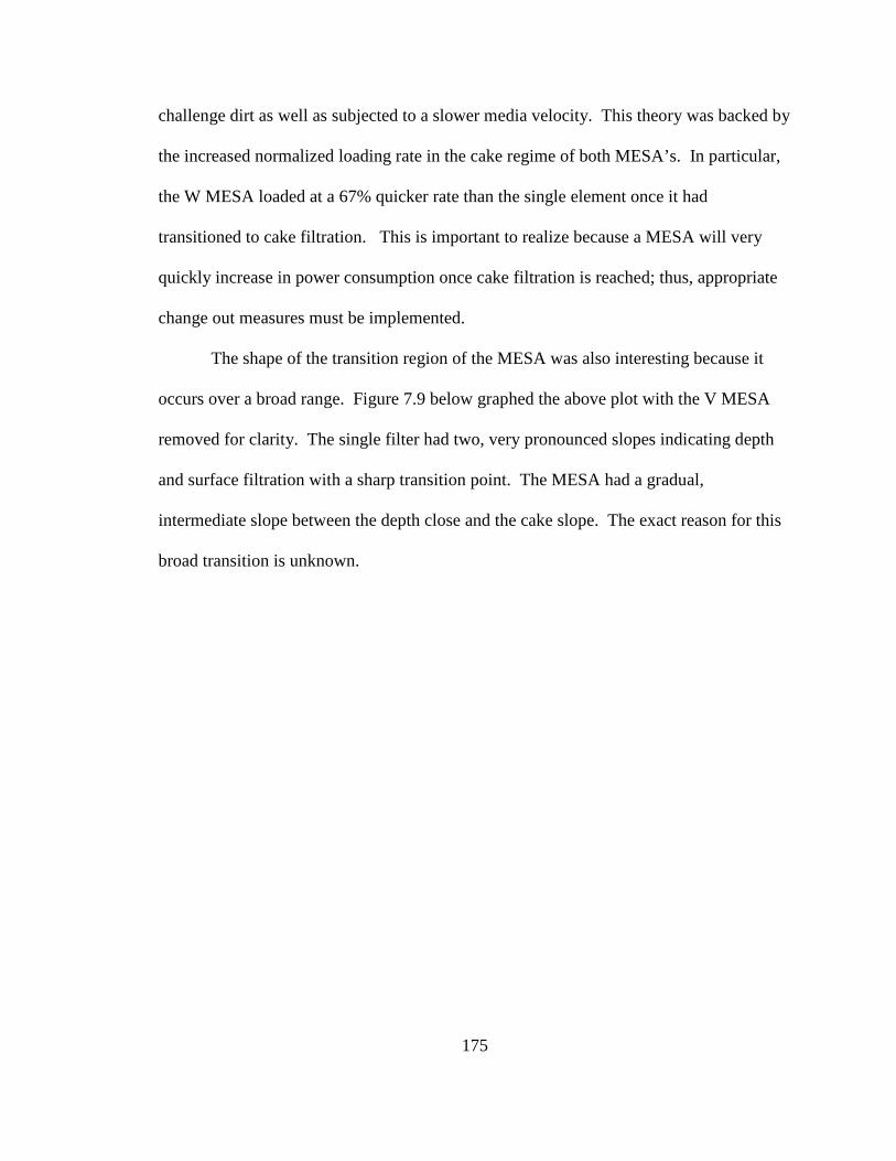
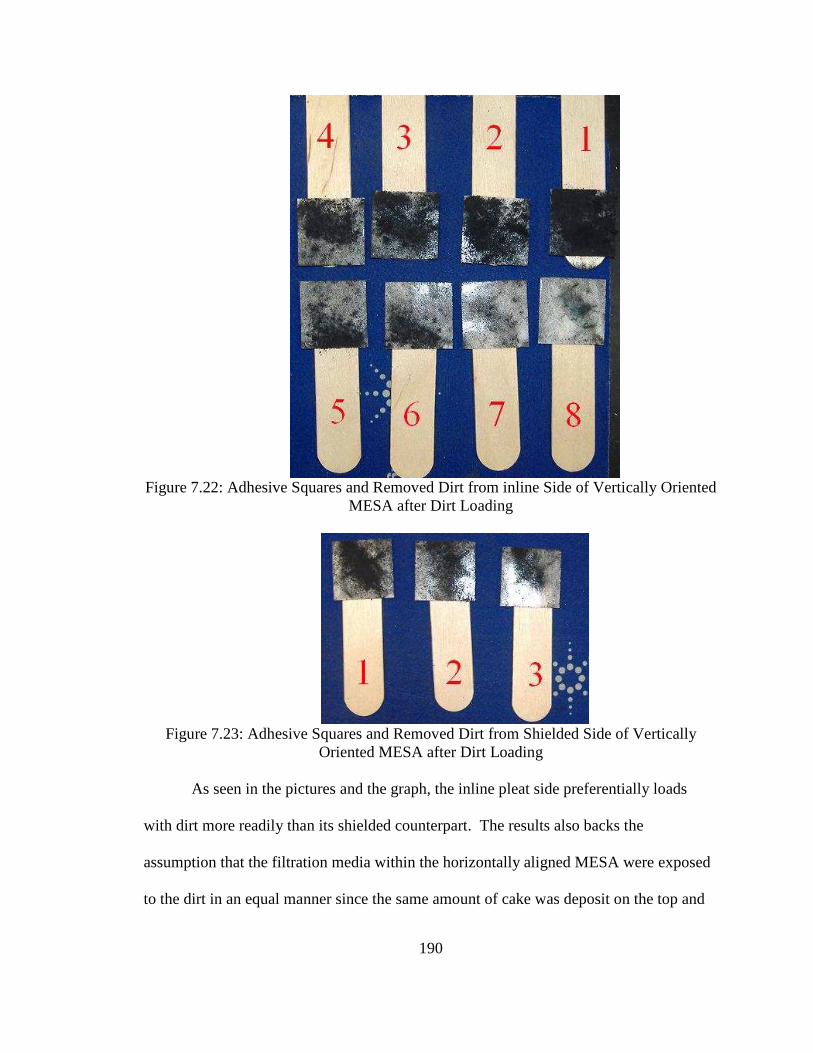
Figure 7.22: Adhesive Squares and Removed Dirt from inline Side of Vertically Oriented MESA after Dirt Loading .............................................................190 Figure 7.23: Adhesive Squares and Removed Dirt from Shielded Side of Vertically Oriented MESA after Dirt Loading .............................................................190 Figure 7.24: Weighed Pulled per Layer of Adhesive Backing .......................................191

Figure A1: Rotameter Calibration Set-Up .......................................................................200

Figure A2: Rotameter Calibration Curve.........................................................................201

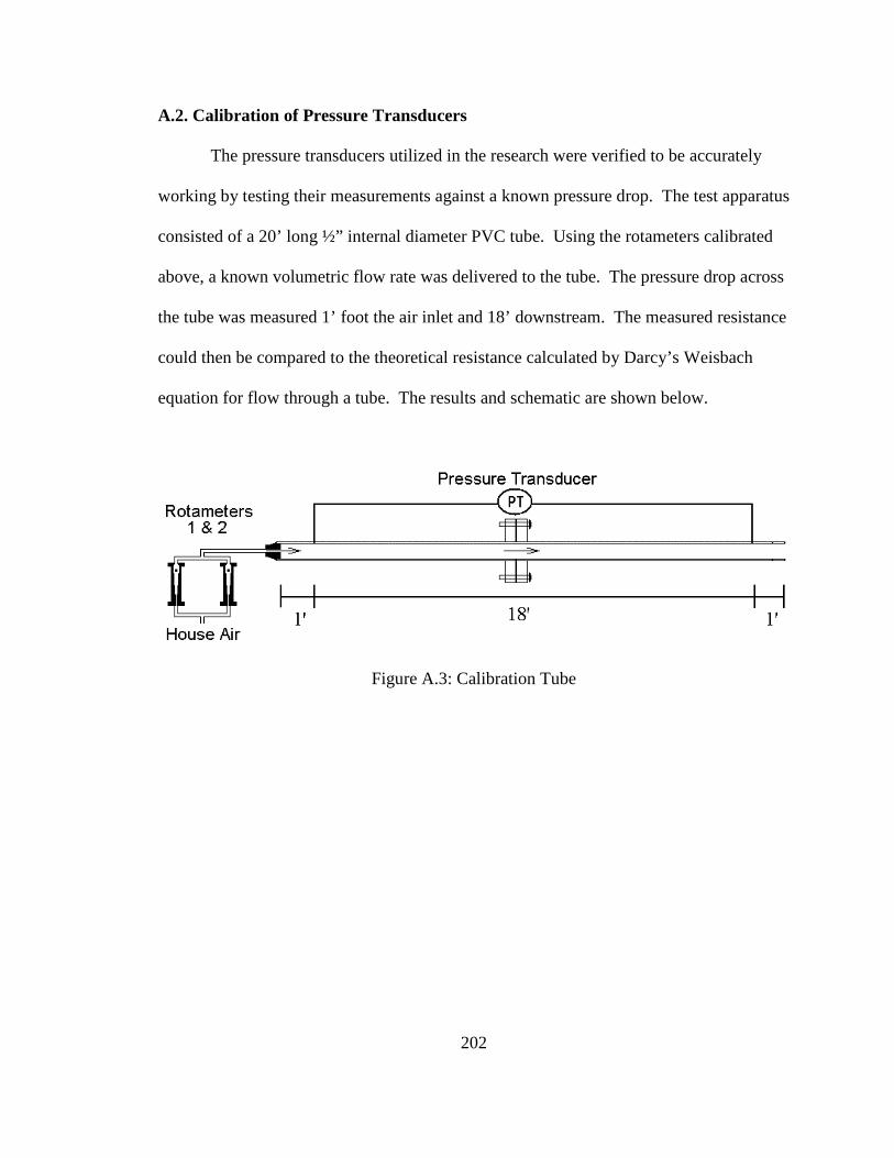
Figure A.3: Calibration Tube...........................................................................................202

Figure A4: Calibration Curve for Pressure Transducer #1 ..............................................203

Figure A5: Calibration Curve for Pressure Transducer #2 ..............................................203

Figure A6: 24”x24”x2” Filter Holder ..............................................................................204

Figure A7: MESA Housing Schematic............................................................................205

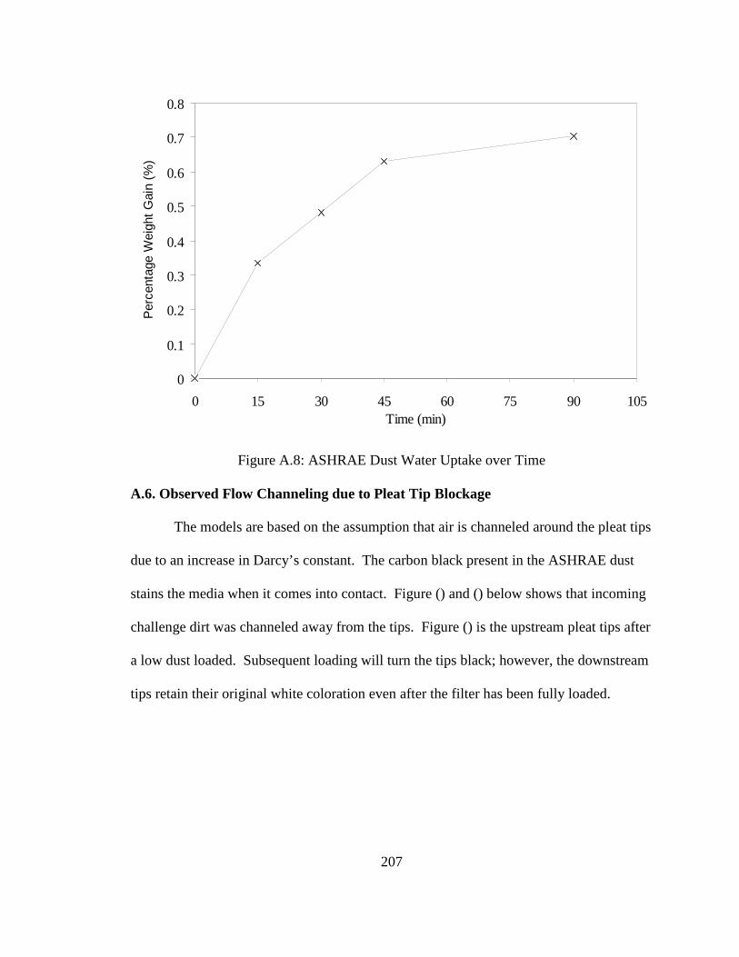
Figure A.8: ASHRAE Dust Water Uptake over Time.....................................................207

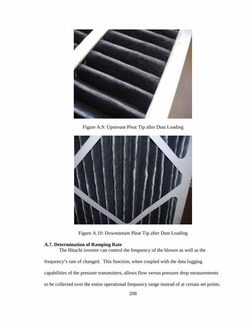
Figure A.9: Upstream Pleat Tip after Dust Loading........................................................208

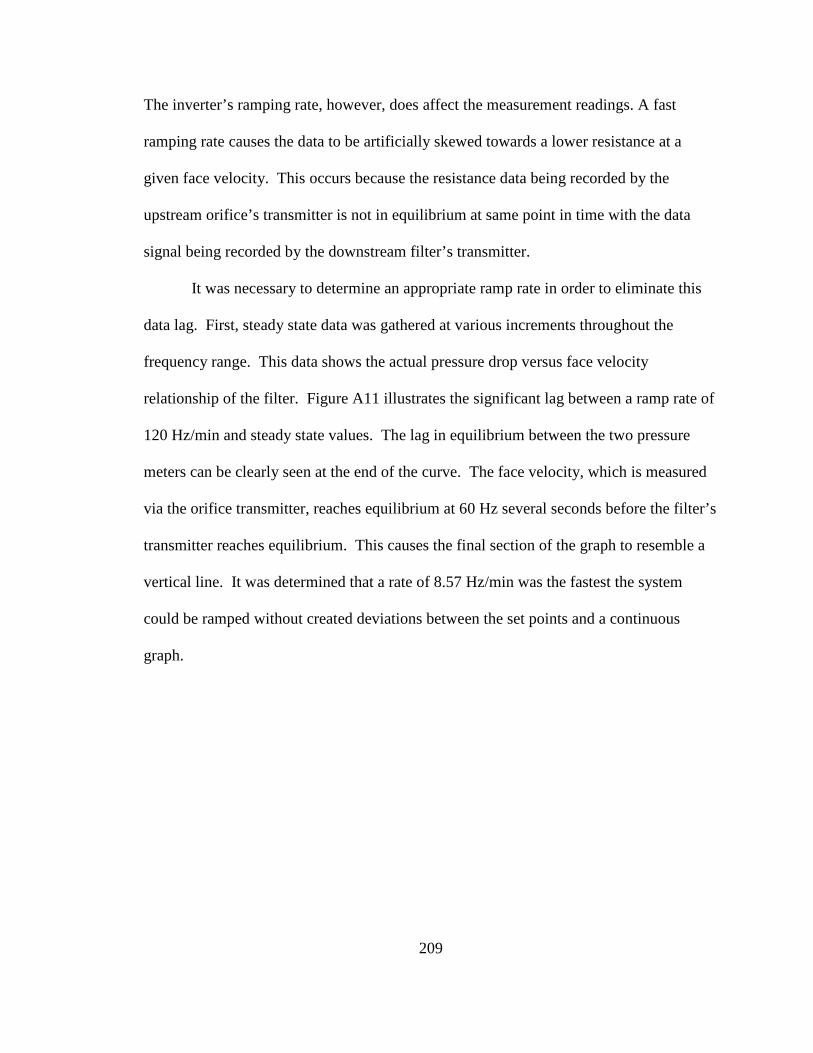
Figure A.10: Downstream Pleat Tip after Dust Loading.................................................208

Figure A.11: Variation in Pressure Measurements due to Incrementing Rate ................210

xxii

LIST OF TABLES

Table 1.1: Minimum Efficiency Removal Value and Typical Filtration Platform..............2

Table 3.1: Summary of Media Constants and Thickness..................................................45

Table 3.2: Summary of Filters Employed..........................................................................53

Table 3.3: Summary of Pleat Coefficients.........................................................................55

Table 4.1: Blockage (FB) Tabulations................................................................................82

Table 4.2: Alpha Tabulations (in radians) .........................................................................82

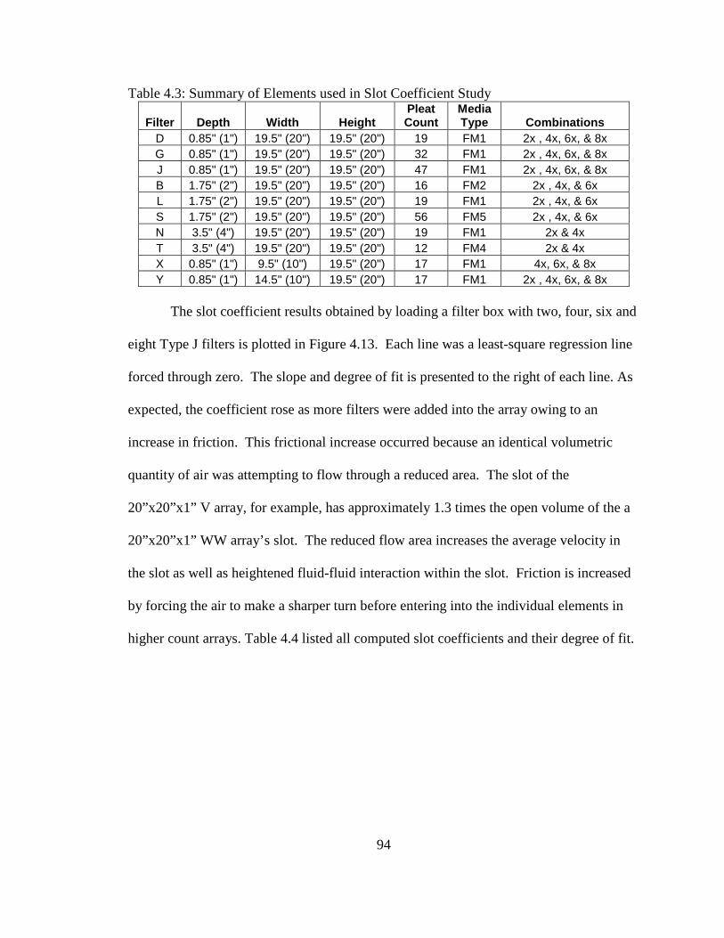
Table 4.3: Summary of Elements used in Slot Coefficient Study .....................................94

Table 4.4: Summary of Observed Slot Coefficients and R2 Fit.........................................96

Table 4.5: MESA vs. Single Filter Comparison ..............................................................106

Table 4.6: Summary of Design Parameters and Effects due to their Increase.................116

Table 5.1: ASHRAE Dust Size Distribution....................................................................127

Table 5.2: Average Velocity and Coefficient of Variation within Test Rig....................128

Table 6.1: Critical Parameters of Filters Utilized ............................................................144

Table 6.2: Interval Loading Rate for 24”x24”x2” 411SF Filter with 15 Pleats ..............159



Table 6.5: Estimated Lifetime Costs for 24”x24”x1” Filters ..........................................161



Table 7.1: Transition Point of V MESA and Single Elements ........................................172

Table 7.2: Associated Costs.............................................................................................177

Table A1: Experimental Data ..........................................................................................201

1

CHAPTER I: INTRODUCTION TO AIR FILTRATION

I.1 Motivation

Adverse health effects stemming from poor indoor air quality (IAQ) has become a

prominent concern since the implementation of energy efficiency buildings in response to

the energy crisis of the 1970s (Kay et al. 1991, Moffat 1997). The decreased exchange

between inside and outside air due to thicker insulation and improved passageway seals

has created an environment were indoor air pollutants can reach levels that are ten times

greater than ambient outdoor conditions (Meckler 1991). The decline in IAQ has been

linked to increases in asthma, allergies, lung/respiratory cancer, and other pulmonary

diseases (Godish 2001). Poor IAQ is also a primary cause for personal discomforts such

as headaches; fatigue; dizziness; nausea; and irritation of skin, eyes, throat, and lungs that

affects the quality of life and worker performance (Moffat 1997). The foremost indoor air

pollutants are volatile organic compounds (VOC’s), ozone, nitrogen oxides, carbon

monoxide, and particulate matter less than 10 microns in diameter (Liu and Lipták 2000).

Since the average American spends an estimated 90% of their time indoor (EPA 2009),

effective air filtration is needed to eliminate these harmful contaminants from human

living environments.

Traditionally, home filters have consisted of a panel units composed of loose

fitting fiberglass fibers. The purpose of these filters was the removal of particles before

they damaged the working machinery of the air handler. Also, the filter prevented the

cooling coils from becoming clogged with dirt which decreases the efficiency of the heat

2

exchangers (Robinson and Ouellet 1999, Waring and Siegel 2008). Panel filters,

however, offer little in terms of removing the serious health affecting particles that are

below 10 micron. Table 1; obtain from the American Society of Heating, Refrigeration,

and Air-conditioning Engineers (ASHRAE) Standard 52.2; highlights some of the

common air filters and their ability to remove particulate matter.

Table 1: Minimum Efficiency Removal Value (MERV) and Typical Filtration Platform

MERV Rating

0.3 to 1.0 Micron

1.0 to 3.0 Micron

3.0 to 10.0 Micron Filter Type

1 n/a n/a < 20% Panel 2 n/a n/a < 20% Panel 3 n/a n/a < 20% Panel 4 n/a n/a < 20% Panel 5 n/a n/a 20 - 35 % Cartridge Filter 6 n/a n/a 35 - 50% Cartridge Filter 7 n/a n/a 50 - 70% Cartridge Filter 8 n/a n/a > 70% Pleated Filter 9 n/a < 50 % > 85% Pleated Filter 10 n/a 50 - 60 % > 85% Pleated Filter 11 n/a 65 - 80 % > 85% Box Filter 12 n/a > 80% > 90% Box Filter 13 <75% > 90% > 90% Bag Filter 14 75 - 85% > 90% > 90% Bag Filter 15 85 - 95% > 90% > 90% Bag Filter 16 > 95% > 95% > 95% Bag Filter

Although higher MERV rated filters excel at removing particulate matter, they

can not remove VOC’s and other airborne molecular contaminants. A second filtration

system, such as a packed bed or monolith, must be employed in order to successfully

remove the non-particulate contaminants. A third option is the utilization of microfibrous

media which has been previously shown to remove many of the airborne molecular

contaminants listed above. Kalluri (2008) demonstrated the ability of microfibrous media

to remove ozone from a polluted air stream. Kennedy (2007) and Queen (2005)

3

employed microfibrous materials in cathode air filters and fire masks for the successfully

removal of VOC’s. Catalyic oxidation of carbon monoxide to the more benign carbon

dioxide has also been achieved through the use of microfibrous media (Karanjjikar 2005).

I.2. Microfibrous Media

Microfibrous Media (MfM) was developed in 1987 for use in chemical and

electrochemical applications by Auburn University’s Department of Chemical

Engineering and the Space Power Institute. The media is a sinter-locked matrix of fibers

with diameters typically ranging between two and twenty microns. Matrices can be

constructed with metal, ceramic, or polymer fibers through a traditional wet-laid paper

manufacturing process. (Tatarchuk et al. 1992, 1994). As the technology developed, the

microfibrous frameworks were used to entrap particles below 300 microns for use in

catalytic and adsorptive applications. The resulting composite structures were known as

Microfibrous Sorbent-Supported Media (MSSM) (Harris et al. 2001).

The ability to be wet-laid and entrap microscopic particles bestows several key

attributes to the media that enhances its utility in sorbent and catalytic processes. The

decreased particle size allows molecules to diffuse into a sorbent’s innermost structure at

a higher rate leading to higher utilization, smaller mass transfer zones, and shorter critical

bed depths compared to packed beds and monoliths (Harris et al. 2001, Kalluri 2008). In

turn, lower amount of costly catalytic material is needed to achieve the same

performance. The wet-lay process creates a homogeneous material that reduces

channeling effects typically associated with the use of sub-millimeter particulate supports

(Kalluri 2008). This assists with preventing the premature breakthrough of the pollutant

4

through the system. The wet-laid process also allows for customizable void volumes

ranging between 30% to 98% (Marrion et al. 1994).

Although MSSM possesses a high contacting efficiency, the drawback to its

utilization as a filtration media is a large pressure drop and relatively low loading

capacity of adsorbent material. The large resistance of the media is due to the

combinational effects of flow through the porous structure and drag forces present on the

embedded particles. The matrix must be composed of micron diameter fibers in order to

entrap the desired range of micro-sized adsorbent particles. The pressure drop of the

media has an inverse quadratic relationship with both fiber radius and particle diameter;

thus, the resistance quickly rises as smaller particles and fibers are employed (Cahela and

Tatarchuk 2001). Capacity of the media remains low due to the thinness of the material

and low concentration of support within matrix. The thickness and support concentration

parameters can be adjusted to increase capacity, but each will cause the pressure drop of

the media to increase in a linear fashion as describe by Darcy’s Law.

Darcy’s Law states that the force required to move a fluid through a porous media

is directly proportional to the media thickness (L), the superficial velocity through the

media (VS), and the permeability constant of the media (Km).

Sm

VK

LghP

µρ =+∆− )( (1.1)

The forces acting on the fluid are pressure (P) and a potential force created on a height of

fluid (h) by the acceleration of gravity (g). The viscosity and density of the fluid flowing

through the media is denoted by µ and ρ respectively. With no elevation change through

the media, the equation can be reduced and rearranged to give the following linear form:

5

Sm

VK

LP

µ=∆ (1.2)

The term µL/Km is known as the Darcy’s constant. Darcy’s Law is generally considered

valid only in the regime of creeping flow (Reynolds Numbers < 1) (Perry and Green

1997). An increase in media thickness or decrease in permeability created by an increase

support concentration will lead to a higher pressure drop of the MSSM material.

I.3. Influence of Pressure Drop within a HVAC System

Proper design of flow resistance is of particular importance in air filtration

applications where a large pressure drop can overload the air handler unit and reduce or

prevent air flow. More importantly, pressure drop is directly related to the energy

consumption of the system. The pressure-volume work of the system can be computed

by (Rudnick 2008):

E = ∆PQt ηB -1 (1.3)

The simple calculation states that the energy (E) required to move the air is the product of

the volumetric flow rate (Q) of air moved, the resistance (∆P), time of operation (t), and

the efficiency of the air handler (ηB). The energy consumption to move the air accounts

for 81% of the total expense in an HVAC system with procurement and additional

operational costs such as labor accounting for the remaining 19% (Arnold et al. 2005). A

significant pressure drop will render a MSSM filtration media impractical due to

substantial operational costs or unfeasible because of the mechanical limitations of the air

handler.

Pleated filters are a platform for improved pressure drop performance and

enhanced capacity of microfibrous materials. The performance enhancements result from

6

transforming the flat material into a three-dimensional, corrugated structure to increase

the available media area. The additional area extends the capacity of a filter as well as

lowers the pressure drop by slowing down the velocity through the porous material. The

addition of each pleat, however, introduces an new source of resistance due to increased

surface-fluid friction. The reduction in pressure drop through the media is steadily

counteracted by a rise in the flow resistance because of increased friction in the pleat.

Due to the exchange of media-induced flow resistance loss for pleat-induced pressure

losses, a pleated filter will experience a minimal resistance corresponding to an optimal

pleat count and media area.

Previous research by Chen et al. (1996), Del Fabbro et al. (2002), Caesar and

Schroth (2002), and Tronville and Sala (2003) each presented plots of pressure drop

versus pleat count that demonstrated this tradeoff behavior (Figure 1.1). Chen labeled the

lower pleat count region to the left of the optimal number as the media-dominated

regime. A filter was listed in the viscosity-dominated regime when it possessed more

than the optimal number of pleats. Although the previous research identified that an

optimal pleat count existed, a detailed understanding of the influential design parameters

and the impact of their variation was not well established.

7

Figure 1.1: Typical “U” Pleating Curve

A need exists for an accurate pressure drop model to assist in designing more

efficient pleated filters. A thorough understanding of the design parameters and their

influence on the overall pressure drop would lead to better predictions regarding the

minimum initial pressure drop or maximum filtration area while maintaining an

acceptable initial resistance that a filter could obtain. A model could be further used to

establish preferred media properties with respect to permeability versus thickness; thus, it

could serve as a design tool for media construction as well. The end benefits to a

filtration design are an increase in dirt holding capacity, improvement in removal

efficiency, and reduction of operational energy costs.

8

CHAPTER II: BACKGROUND AND EXPERIEMTNAL

FOR MODELING INITIAL PRESSURE DROP

II.1. Previous Pleated Filter Models

Various models have been published that calculate the flow resistance

encountered within a pleated filter. Chen et al., Rivers & Murphy, Tronville & Sala,

Caeser & Schroth, Del Fabbro et al., and Raber have each suggested that a pleated filter

can be modeled by the general formula:

∆Pf = KGEOV2F + KMVM (2.1)

The equation states that the total pressure drop across the filter (∆Pf) is a second order

polynomial composed of a geometric and media term. The geometric term is equal to the

squared face velocity into the filter (VF) multiplied by a geometry coefficient (KGEO).

The media term is composed of the media velocity (VM) times the media coefficient

(KM). The media velocity is calculated by dividing the face volumetric flow by the

available filtration area. The following sections briefly discuss each researcher’s work

and their methods to model a pleated filter.

II.1.1. Chen et al.

Chen et al. (1995) calculated the pressure drop of a rectangular pleated filter

through the use of a nine-node finite numerical method. The flow resistance upstream

and downstream was computed by the Navier-Stokes equation. The pressure loss

9

through the media was estimated by Darcy-Lapwood-Brinkman equation with the media

constant (K) experimentally determined.

Co

thMCMf V

P

MPVKPPP µµ

−+=∆+∆=∆

2 ¼ (2.2)

The research proposed that the optimal pleat count existed when the resistance of

the media equaled that of the viscous effects. This computation is displayed by Equation

2.3 and is rearranged into a general correlation as shown. Once the correlation

coefficient (C) is calculated, the optimal pleat count can be computed for a given media.

−+=

∆∆+=

∆∆

3

2

) ½(

811

to

h

M

C

M

fo

MP

P

KC

P

P

P

P (2.3)

Besides experimentally determining the media coefficient (K), all work presented

in the first study was theoretical. When Chen et al. (1996) subsequently investigated the

flow resistance through a triangular pleated filter, the research concluded that the face

velocity explored in the first study [<100 feet per minute (fpm)] was not a reasonable

operational value. The use of Darcy-Lapwood-Brinkman equation was found to be

invalid in the new operational velocity range. The researcher replaced the equation with

a semi-empirical model:

2

o2

o1 ½P

2

½P

21

∆+

∆+=

∆∆

MMM

f

PM

PM

P

P (2.4)

The last term in Equation 2.4 is proposed to account for viscous effects that stem

from the directional flow change inside the pleat. Chen concludes that the angle of

change is influenced by the media’s resistance; therefore, M2 must be empirically solved

for each media type used.

10

II.1.2. Rivers & Murphy

Rivers and Murphy (2000) proposed a modified version of Equation 2.1 that

could be used to model the total pressure drop through any air filter.

∆Pf = KGVNf + f(Vm, µ, αSM, β, Mt, Rf, Kn, M) (2.5)

The work primarily focused on estimating the media’s resistance. In particular, the

research investigated how the compression of an HVAC media led to non-linear rises in

resistance as face velocity was increased. The model provides great detail into predicting

media performance based on the media design parameters of media velocity, viscosity,

volumetric solid fraction, media non-uniformity, media thickness, fiber radius, Knudsen

number, and dust load (denoted in order as Vm, µ, αSM, β, Mt, Rf, Kn, M). To account for

the influence of geometric factors, the model relies on two non-transferable factors

lumped into a bulk term (KGVNf) that must be empirically fit for each filter. The process

first determined ∆Pf versus face velocity for a filter, and then Equation 2.5 was

rearranged into a linear form to solve the constants N and KG. Reported N values varied

from 1.15 to 3.74 while the KG values were not discussed. The model can not be use in a

predictive capacity since the factors must be empirically determined for each filter.

II.1.3. Del Fabbro et al.

Del Fabbro et al. (2002) focused on modeling pressure loss created within a

pleated filter composed of HEPA and low efficiency filter medium. The research initially

attempted to compare experimental data to a computational fluid dynamic (CFD) model.

The CFD model was ultimately deemed too computational expensive and difficult for the

accuracy of results it provided. The study turned to a semi-empirical, dimensionless

model that identified and utilized the following eight critical design parameters: pressure

11

drop, filtration velocity, media resistance, media thickness, density, viscosity, pleat

height, and pleat opening.

The model could theoretically predict pressure drop through a pleated filter if the

critical parameters are known or specified; however, the model was shown to be

incapable of accurately predicting the experimental data presented by Del Fabbro. The

results displayed significant positive and negative deviations between experimental and

modeled data with divergences as large as 100 Pa (0.4” H2O) and 500 Pa (2” H2O).

Beyond the strong deviations, the flow conditions studied were far below a normal filter’s

operating range. The maximum, modeled face velocity of 15 cm/s (30 fpm) was an

order of magnitude below standard operational conditions. The study also failed to

account for the pressure drop associated with the filter’s housing.

II.1.4. Caeser and Schroth

Caeser and Schroth (2002) created a three termed model for predicting pressure

drop in deep-pleated (4 to 12 inches) filters. The three resistances were the influence of

airflow in and out of the pleats, through the pleats, and through the media. The airflow in

and out of the pleats was modeled by a coefficient of friction. A reduced Navier-Stokes

equation was used to compute pressure drop through the pleats. The media’s resistance

was calculated by Darcy’s Law. The total resistance of a filter was the summation of the

three terms.

Although the methodology employed by Caeser and Schroth was unique, the

research overall had several deficiencies. The coefficient of friction listed in the research

resembles a sudden contraction modified by a second parameter. The second parameter

was listed as a function of entry and exit edge sharpness, yet a means to calculate the

12

second parameter was not presented. The study focused on deep-pleated HEPA and

ULPA that are commonly built with metal spacers/combs to keep the pleats from

collapsing, yet the model lacks a method to account for the influence of these additional

structures. Several assumptions are postulated to reduce the Navier-Stokes equation into

a more computationally simple form. The validity of these assumptions was never

proven against experimental data.

II.1.5. Tronville and Sala

Tronville and Sala (2003) expanded on Equation 2.1 by proposing two new

formulas to calculate the coefficients. Following the research of Rivers and Murphy, the

pressure drop for flow through the media (1/Kc) was modeled by the Carmen-Kozeny

equation with the solid mass fraction (α) described by the Natanson – Pich function. The

parameter Dc is the pore hydraulic diameter and ∆z is the thickness of the filter. The

geometric resistance coefficient (1/Kair) was based on the pleat count per unit length (σ)

raised to an empirically determined power N multiplied by the face velocity. Equation

2.6 is the end result of substituting the new coefficients into Equation 2.1. The two

unknowns (N and Dc) can be solved by plotting a second-degree polynomial to

experimental data obtained for a filter.

D

C

NDD U

zD

fUU

KcKairz

P µσ

ασµ

∆+=

+=∆∆−

2

)(211 (2.6)

The research only empirically determined the coefficients for a single filter. The

authors assume that determining the parameter N at one pleat configuration would allow

them to assess geometry resistance effects at all pleat arrangements. The minipleat style

filter in this study possessed 304 pleats per meter, yet the model makes predictions for

13

pleat counts upwards of 1000 pleats per meter. With no supplementary experimental data

to back this claim, the assumption that the model is capable of making this prediction

becomes questionable. Furthermore, the model makes no concessions to account for

filter housing or variations in filter depth.

II.1.6. Raber

Raber (1982) attempted to establish the effects of dirt loading on the flow

resistance within a pleated filter. The media’s resistance was experimentally identified

by testing a small media sample to determine the impact of dust loading on the pressure

drop. The term was found to be a second order polynomial that increased as the sample

was loaded with dirt. The geometric resistances were numerically calculated from the

momentum balance based on a characteristic half-pleat control volume. The half pleat

was divided into five elements, and the total resistance across the half-pleat was

calculated by sequentially solving the momentum balance with the conservation of mass

equation and the media influence polynomial.

To assess the validity of the calculations, Raber built four 24”x24”x12” (HxWxD)

prototype filters that possessed 16 pleats. The filters were tested at a face velocity of 500

fpm and loaded with dust until a final resistance of 1” H2O was reached. The prototypes

were not accurately modeled by the calculation. The initial deviations were

approximately 0.05” H2O to 0.1” H2O and grew beyond 0.2”H2O as the filters were

loaded.

A probable source of error is the elimination of the friction term from the

momentum balance. The research dismisses the friction losses due to the relatively

moderate velocities encountered within the pleat. The moderate velocities, however, are

14

the product of employing 128 square feet of media to reduce the face velocity from 500

fpm to 3.9 fpm. The assumption’s dismissal becomes increasingly debatable when

attempting to model shallower filters with substantially higher pleat velocities.

Although Raber does not incorporate friction losses into his model, he does

outline seven areas that would be associated with friction loss. This outline, described in

Section 3.I.C, serves as the basis for the flow pattern used in this research.

II.2. Objectives of Current Modeling Efforts

The overarching goal of this work is the formulation of a model that meets the

key objectives described below. The study was deemed necessary since the prior models

often fail to achieve two or more of these requirements. The sixth objective is unique to

this research, and no previous work regarding this subject was found.

1. Predictive

The model should be capable of predicting total pressure drop based solely on

geometric design and media properties. The use of non-transferable factors should not be

utilized. In particular, a model should not need empirical pressure drop versus face

velocity data from a fully-constructed filter in order to make predictions.

2. Full Accounting of Design Parameters

The model should meticulously account for all previously identified contributing

design parameters. The inability to properly assess the design parameters results in

misattributed resistances and erroneous predictions. The most commonly ignored design

parameters are the contribution of pleat tips to the overall resistance and the effect of

structural elements within the filter.

15

3. Accurate

The ability to accurately predict a desired behavior is the primary objective of any

modeling endeavor. A model should be able to predict the initial pressure drop of a filter

to within ±10% for a given operational velocity.

4. Experimentally Verified

An empirical model should be based upon observed data covering a wide range of

all design variables. A theoretical model needs to be tested against a similarly diverse

field of design variables.

5. Computationally Benign

The model allows for quick calculations to improve the utility of the model. Long

computation times and exceeding complex mathematics can hinder the usefulness of a

predictive model.

6. Adaptable

The model should be able to make predictions for a single pleated filter as well as

a Multi-Element Structured Arrays (MESA’s). Multi-Element Structured Arrays are a

novel filtration platform that incorporates numerous filter elements together to further

reduce the pressure drop and drastically increase the available media area. The model

should fulfill requirements 1 through 5 for both types of filtration systems.

II.3. Theory

The following equations are used in the research and modeling efforts:

Forchheimer-extended Darcy’s Law, Bernoulli’s Equation, the Equation of Continuity,

and the Momentum Balance. Several previously published coefficients of friction are

employed in conjunction with Bernoulli’s equation.

16

II.3.1. Forchheimer-extended Darcy’s Law

The high operational velocities associated with a particulate air filter often result

in non-linear deviations from Darcy’s Law for flow through the media (Rivers & Murphy

2000, Chen et al. 1996). Rivers & Murphy concluded that the deviations were the

product of media compression due to the air’s inertial force being sufficient to compress

the fibers together. Although Darcy’s Constant should be slightly decreased due to the

overall reduction in length of the porous media, the compression changes the internal

void volume and tortuosity of the media leading to higher superficial velocities,

decreased permeability, and an overall increase in Darcy’s Cconstant.

A practical method to account for the non-Darcian behavior is the addition of a

second-order term to Darcy’s Law (Scheidegger 1974). Equation 2.7 is known as a

Forchheimer-extended Darcy’s law. The “A” term is equivalent to the Darcy’s Law

constant (µL/Km). The “B” constant accounts for the non-linear deviation due to inertial

effects.

∆P = AVM + BVM2 (2.7)

Numerous theoretical equations exist that attempt to relate the physical

significance of the second media constant, but these theories require extensive knowledge

of the media’s fiber dimensions and packing densities (Rivers & Murphy 2000). The

research presented by Rivers and Murphy demonstrates the complexity and difficulty in

accurately modeling media performance with these theories. Since the primary objective

of the research is to identify and determine the resistances created by the geometric

design parameters and not the media formulation, it is preferable to model the media

constants by a quick, empirical approach that will not introduce as much theoretical error.

17

The second order term also allows the model to account for the presence of particle

matter embedded within the fibrous framework.

II.3.2. Mechanical Energy Balance / Bernoulli’s Equation

The mechanical energy balance is a summation of kinetic, potential, mechanical,

compressive, and viscous energy terms. Bernoulli’s Equation is a specialized case of the

mechanical energy balance. Bernoulli’s Equation assumes incompressible, steady-state

flow while maintaining a control volume with stationary, solid boundaries (Perry and

Green 1997). Bernoulli’s Equation is:

P1/ρ + αVV12/2 + gZ1 + δWs = P1/ρ + αVV2

2/2 + gZ2 + Lv (2.8)

Rearranging similar terms:

∆(P/ρ + ½αV2 + gZ) = δWs – Lv (2.9)

Equation 2.5 states the change in pressure, kinetic energy, and potential energy is

equal to the mechanical energy (δWs) added to the system minus the viscous losses (Lv).

The term alpha (αV) is the ratio of velocity cubed over the average velocity cubed. Alpha

assumes a value of unity for turbulent flow. Bernoulli’s Equation can be further

simplified by eliminating elevation change within the control volume and removing all

mechanical work. The following equation results when applied between two points:

∆P = P1 – P2 = ½ρ (V22 – V1

2) + Lv (2.10)

The viscous loss term (Lv) accounts for the change of mechanical energy into

heat due to viscous forces. The term is also referred to as the minor or miscellaneous

losses. Denoting the viscous losses as minor or miscellaneous is misleading because they

are frequently the primary resistance forces within a system (Perry and Green 1997).

There are two methods to account for the losses: equivalent length or velocity head. The

18

later will be used in this dissertation. The Lv term can be reported in equivalent number

of velocity heads.

Lv = ½ρ KV2 (2.11)

The K value is referred to as either the velocity head loss coefficient or the

coefficient of friction. Although the viscous losses can be theoretically computed by

simultaneously solving both the mechanical energy balance and momentum balance for

the given control volume, they are most often determined through experimental

measurements (Bird et al. 2001, Perry and Green 1997). The coefficient is required to be

a dimensionless function of either geometry, Reynolds number, or both. The importance

of the Reynolds number increases in laminar flow due to the rise in friction at the

boundaries (Bird et al. 2001). The V term is an arbitrary, reference velocity on which the

coefficient is based.

The present research makes use of the following five previously researched

friction coefficients: sudden contractions, sudden expansions, gradually contractions,

flow across a perforated plate, and flow through a duct. Each coefficient’s formula,

general control volume schematic, and reference velocities are presented below.

19

1. Coefficient of Friction for a Sudden Contraction

Idelchik (1994)

Figure 2.1: Sudden Contraction Diagram

0.75

1½

−=

LARGE

SMALLC A

AK (2.12)

(Based on downstream velocity)

2. Coefficient of Friction for a Sudden Expansion

Idelchik (1994)

Figure 2.2: Sudden Expansion Diagram

2

1

−=

LARGE

SMALLE A

AK (2.13)

(Based on upstream velocity)

20

3. Coefficient of Friction for a Gradually Contraction

Fried and Idelchik (1989)

Figure 2.3: Gradually Contraction Diagram

KGC = [(-0.0125N4 + 0.0224N3 – 0.00723N2 + 0.00444N - 0.00745)(A3 - 2πA2 – 10A)] (2.14)

A = 0.01745θ (where θ is in radians) N = A2 / A1

(Based on upstream velocity)

4. Coefficient of Friction for Flow Across a Perforated Plate

Idelchik (1994)

Figure 2.4: Grating Diagram

2

707.1−

−=

TOTAL

FREE

TOTAL

FREEG A

A

A

AK (2.15)

(Based on downstream velocity)

21

5. Darcy-Weisbach Equation: Flow in a Duct with Smooth Walls

Idelchik (1994)

Figure 2.5: Duct Diagrams

λ

=

hT D

LK (2.16)

(Based on flow velocity)

l = 64/Re Re < 2000 (Laminar Regime)

( )

−×=

264.1log(Re)8.1

1λ Re > 4000 (Turbulent Regime)

νhVD

=Re (2.17)

Tabular data is available in the Handbook of Hydraulic Resistance (Idelchik

1994) for computing λ in the transitional regime defined by Reynolds number between

2000 and 4000.

II.3.3. Equation of Continuity

The equation of continuity is based on the conservation of mass (Perry and Green

1997). The equation denotes that mass flow entering and leaving a control volume is

equal. When constant density is assumed, the equation can be written as:

V1 A1 = V2 A2 (2.18)

22

II.3.4. Momentum Balance Although not extensively used in the study, the momentum balance is:

mgFuAPuAPuAVuAVdt

dS ++−+−=Γ 22211122

22211

211 ρρ (2.19)

The balance asserts that the change of momentum is the difference between the amount

of momentum carried into the system by the fluid and the pressure acting on the fluid

versus the momentum carried out by the fluid and the pressure acting on the outlet fluid

(Bird et al. 2001). Addition factors such as the force of gravity on the fluid’s mass and

the force of system’s surfaces on the fluid (Fs) are factored into the balance.

II.4. Experimental Setups

Two separate test rigs were constructed and used to measure pressure drop

performance across a media sample and a filtration system. A general description of the

test rigs, control runs, and equipment verification are provided in this section.

II.4.1. Media Test Rig

The media constants were determined using a 1-inch circular diameter duct

powered by house air at 100 psig (Figure 2.6). The duct length to diameter ratio was

sufficiently long (48-to-1) to ensure no entrance effects. A media sample was held in

place by two plates tightened together by four nut and bolt assemblies. A twelve inch

outlet section was located downstream of the media sample to prevent additional pressure

loss due to a sudden expansion out of the tube.

23

Figure 2.6: General Schematic of Media Test Rig

Airflow to the rig was controlled by two rotameters. The rotameters were

connected in series to produce a stable, controllable volumetric flow between 0 and 160

SCFH. This correlated to a maximum superficial velocity of 488.9 fpm within the one

inch test rig. The rotameters were calibrated by a volumetric displacement test (See

appendix for calibration procedure and results). Resistance measurements were obtained

with an Omega Model PX154–010DI differential pressure transmitter connected to a

pressure tap located two inches upstream and five inches downstream of the media

sample. The taps had a one-eighth inch diameter and were drilled flush with the inner

tube diameter to prevent increased friction. The pressure transmitter had a range of -1.0

to 10” H2O with a resolution of 0.001” H2O.

A control test performed on the media test rig resulted in 0.003” H2O of pressure

drop at the maximum volumetric flow. The measured resistance follows the Darcy-

Weisbach Equation (Eq. 2.16) for flow in a circular pipe with a smooth interior. The

measured and calculated values are shown in Figure 2.7. The step-shaped appearance of

24

the measured data was the product of the differential pressure transmitter’s resolution of

0.001” H2O. The slope shifts in the calculated plot were due to the transition from

laminar to turbulent flow.

0

0.001

0.002

0.003

0.004

0.005

0 100 200 300 400 500 600

Face Velocity (fpm)

Pre

ssu

re D

rop

("

H2

O)

Measured Data

Darcy-Weisbach Calculation

Figure 2.7: Control Pressure Drop Curve for Media Test Rig II.4.2. Filtration Test Rig

A general schematic of the filtration test rig is depicted by Figure 2.8. The test rig

was composed of the following eight subunits: (1) blower, (2) blower sleeve, (3) three-

way transition, (4) baffles, (5) air straighteners, (6) main duct, (7) filter box, and (8)

outlet duct. The primary building material was 5/8” thick particle board. The subunits

were fastened by nut and bolt fixtures. All joints were sealed with a polymer glue gun.

The edge of each section was fitted with ¼” foam weather-stripping. After tightening the

bolts to compress the weather-stripping, the resulting seal produced no noticeable leaks.

25

Figure 2.8: General Schematic of Blower Test Rig

The air handler used was a Dayton System with a 15” impellor powered by a 3 Hp

Hitachi motor. The motor was controlled by a Hitachi frequency drive with a range of

zero to sixty hertz at 0.1 Hz increments. The outlet port dimensions for the blower were

16” x 11.5”.

A sleeve served as a connecting segment between the blower and the three-way

transition. The sleeve was attached to the blower’s outlet port. A pressure tap, located

on the sleeve, coupled with a pressure transducer monitored resistance across the blower.

Once inside the three-way transition, the cross-sectional dimensions expanded from 16” x

11.5” to 19.5” x 19.5” (H x W). The three-way transition then connected to the baffles.

The baffles were composed of 4 vertical planks followed by 4 horizontal planks.

This created an outlet composed of twenty-five squares. The allowable flow to each

square was controlled by the position of the vertical and horizontal planks. The baffles

were followed by the flow straighteners. The first straightener was a perforated metal

plate that blocked fifty percent of the cross-sectional area. The second straightener was a

heavy mesh screen. The airflow passed from the straighteners into the main duct. The

main duct was composed of three extensions. It had a length of twelve feet with internal

dimensions of 19.5” x 19.5” (H x W).

26

The baffles, flow straighteners, and main duct served to delivery a uniformly-

distributed airflow into the filter box. The baffles directed large quantities of air to the

desired segments of the duct. The straighteners assisted with leveling the flow by

introducing a considerable resistance into the system. The length of the main duct

allowed the air to evenly disperse. The before-and-after effects of adding these subunits

are highlighted below. The figure was created by measuring velocity at each point

depicted by the 7x7 grid with a hot-wire anemometer (Extech Model # 407123). Without

any duct modifications, the blower delivered a heavily concentrated volumetric flow to

the left-hand side of the ductwork. The distribution system eliminated this “hot spot” and

reduced the variation between the maximum and minimum localized velocity by an order

of magnitude.

Figure 2.9: Flow Distribution at 40 Hz Before (A) and After (B)

Once it had traveled through the main duct, the air entered into the filter box. The

filter box could be loaded with a single filter or a multi-element pleated filter array. The

filter box had the following dimensions: 19.5”x19.5”x 24” (HxWxL). The top of the

filter box contained a window in order to observe that the pleat’s integrity remained intact

27

throughout the experiments. The filter box was followed by the outlet section. The 24”

long outlet section prevented an increase in pressure drop due to sudden expansion out

into the room.

A metal strip was positioned four inches from the front of the filter box to secure

a single filter into position. The strip had a height of 1/8” that allowed it to fit behind the

filter’s housing without interfering with the pressure measurements. For array tests, the

filters were held together and sealed into place using duct tape. No additional support

was needed to keep the filter array in position due to the tight fit of the filter box.

Pressure drop across the filtration section was monitored by a Dywer Mark II

monometer and an Invensys Foxboro IDP10 differential pressure transmitter. The

equipment was connected upstream into the duct by three pressure taps located ten inches

before the filter test box. A 1/8” pressure tap located in the center of the duct was

connected to the manometer. The manometer’s second connection was left open to the

room’s atmosphere. The other two pressure taps were evenly spaced across the top of the

duct. The taps had a 1/4” opening within the duct that reduced to a 1/8” tube fitting. All

taps were drilled flush to the ducts interior wall to prevent additional friction. The two

taps were connected together via a “T” junction. The line was then ran to the differential

pressure transmitter. The transmitter’s outlet was connected to a second “T” junction.

The “T” split lines were connected downstream to pressure taps located six inches before

the duct outlet. The dual tap configuration was a method to average the pressure drop

readings.

Air to the blower was drawn from the room. All tests were performed in an

environment of approximately 20°C (68 °F) and elevation of 215 meters (705 ft) above

28

sea level; therefore, the density of air was assumed to possess a constant valve of 1.16

kg/m3 (0.0725 lb/ft3) throughout the experiments.

The ASHRAE 52.2 Standard provided an outline for certifying an acceptable flow

distribution and pressure drop across an empty test section. The flow distribution test,

outlined in Section 5.2, consisted of a nine-point test at three volumetric flow rates (472,

1970, and 2990 cfm) (ASHRAE 2007). A nine square grid was bracketed off at the

outlet of the duct with a thin metal wire. The average velocity was taken at the center of

each grid square for one minute. The test was repeated three times at each square. The

square’s velocity value was composed of the average from the three tests. The

coefficient of variance was computed between all nine squares at a given volumetric flow

rate. The coefficient of variance was defined as the standard deviation between the nine

points divided by the mean. The coefficient of variance must be less than ten percent to

pass. Data and the coefficients of variance for the ductwork utilized in this study were

presented in Figure 2.10. The velocities units were listed in meter per second (m/s).

Figure 2.10: Coefficient of Variance

Section 5.16.2 of ASHRAE Standard 52.2 states that the pressure drop across the

test section at 1970 cfm (500 fpm in a 2’x2’ duct) shall be less than 0.03” H2O (ASHRAE

29

1999). The test rig’s recorded pressure drop was approximately 0.001” H2O at the

volumetric flow of 1970 cfm.

As with the media test rig, the pressure drop between the pressure taps was

adequately calculated by the Darcy-Weisbach equation. The results of the control run

and the calculated values were presented in Figure 2.11. The step-like distribution of the

measured values was due to the pressure transmitter’s resolution of 0.001” H2O. The

transition from laminar to turbulent flow was not observed in the control plot because it

occurred at 24 fpm. Since the flow was primarily turbulent in the ductwork, the alpha

term in Bernoulli’s Equation equaled unity.

0

0.001

0.002

0.003

0.004

0.005

0 200 400 600 800 1000 1200Face Velocity (fpm)

Pre

ssu

re D

rop

("

H2

O)

Measured DataDarcy-Weisbach Calculation

Figure 2.11: Control Pressure Drop Curve for Filter Test Rig

30

II.5. Data Acquisition

II.5.1. Media Pressure Drop Curves

Three pressure drop runs were performed on each media sample. The first run

consisted of 35 data points, the second run 12 data points, and the third run 11 data

points. A data point consisted of setting the rotameter to a flow rate and recording the

corresponding pressure drop. Each run used a different strategy for incrementing the

rotameters to randomize the data collection.

II.5.2. Filter Pressure Drop Curves

All data collected during a single filter experiment followed the manner described

below unless stated otherwise. The blower frequency was first set at 5 hertz, and the flow

was allowed to equilibrate. The pressure drop across the blower was measured by the

pressure transducer. The pressure drop across the filtration section was measured by the

differential pressure transmitter and manometer. An average velocity was measured with

an Extech Model 451104 vane-anemometer over a thirty second period by uniformly

moving the meter over the path indicated below at the outlet of the test rig. This

measurement technique was based on the ASHRAE 52.2 velocity uniformity test.

31

Figure 2.12: Measurement Path for the Vane Anemometer

The measurements were repeated at the following frequencies in the order listed:

10, 15, 20, 25, 30, 35, 40, 37.5, 32.5, 27.5, 22.5, 17.5, 12.5, and 7.5 hertz. The test was

repeated up to three times on certain filters, but multiple runs were ultimately abandoned

due to time constraints. Frequencies above forty hertz were not measured during single

filter tests because they corresponded to velocities greater than 1000 fpm. Frequencies

below five hertz were not measured in either filter arrangement because the blower was

not able to overcome the initial flow resistance created by the test rig; therefore, there

was no flow in the ductwork.

For the multi-element test, data was collected in the same manner up until 35

hertz. Frequencies larger than 35 hertz corresponded to face velocities greater than 1000

fpm. The frequency was then decreased in a following manner: 33.7, 32.5, 31.3, 28.7,

27.5, 26.3, 23.7, 22.5, 21.3, 18.7, 17.5, 16.3, 13.7, 12.5, 11.3, 8.7, 7.5, and 6. 3 hertz.

Only the pressure drop measurements were recorded as the frequency was decreased.

32

This was done to save time on data recording since the velocity could be accurately

calculated from the blower curve based on pressure drop data (Figure 2.13).

Once the data was collected for a filter or array, a pressure drop curve was created

by plotting pressure drop versus face velocity. A regression line was fitted to each

pressure drop curve for use in data analysis. The fitted line helped alleviate individual

data discrepancies. The Darcy-Weisbach equation was used to remove the background

noise from the measurements.

As stated, the velocity values were computed from the blower curve in multi-filter

tests. The volumetric flow could be calculated based on the pressure drop across the

blower and frequency setting by the following series of equations:

i) RPM = 37.75 x Setting (Hz) Rate per Minute ii) k = RPM / 2265 (Hz) k Factor iii) ∆P60Hz = ∆Pblower / k

2 Pressure Drop at 60 Hz iv) V60 Hz = -25.32∆P60Hz

2 – 389.08∆P60Hz + 5185.5 Volumetric Flow at 60 Hz v) V = kV60 Hz

Volumetric Flow at Setting Once the volumetric flow was known, the face velocity was calculated by dividing the

volumetric flow by allowable flow area. Figure 2.13 was a comparison of 189 velocities

measured by the vane-anemometer and the resulting calculations from the blower curve.

33

y = 0.9816x

R2 = 0.9914

0

100

200

300

400

500

600

700

800

900

1000

0 200 400 600 800 1000

Velocity Computed by Vane Anemometer (fpm)

Vel

ocity

Com

pute

d by

Blo

wer

Cur

ve (

fpm

)

Figure 2.13: Velocity Measurement Comparison

The measurement comparison between the differential pressure transmitter and

the manometer was shown in Figure 2.14. The meters showed a one-to-one

correspondence. The figure developed a plateau-shaped distribution as pressure drop

increased. This was due to the gradual decrease in manometer resolution at readings

above 0.1” H2O.

34

y = 1.0098x

R2 = 0.9978

0

0.2

0.4

0.6

0.8

1

1.2

0 0.2 0.4 0.6 0.8 1 1.2

Differential Pressure Transmitter Measurement (" H2O)

Man

omet

er M

easu

rem

ent

(" H

2O)

Figure 2.14: Pressure Measurement Comparison between Manometer and Transmitter

II.5.3. Media Thickness The media thickness was determined with a micrometer. A given media was

layered twenty times, and the thickness was measured. The test was repeated twice, and

the average thickness of a single layer was calculated from the three tests.

35

CHAPTER III: INITIAL PRESSURE DROP MODELING

OF PLEATED FILTERS

III.1. Introduction

III.1.1. Pleated Filter Schematics

The following schematics (Figure 3.1, 3.2, & 3.3) are provided to familiarize the

reader with the dimensions and nomenclature used throughout the research to describe a

pleated filter. Figure 3.1 is an illustration of a filter with nine pleats. The symbols FD,

FH, and FW stand for filter depth, filter height, and filter width. A filter will often be

referred to as an “X” inch filter. This size dimension denotes the filter depth. The face

dimensions (FH and FW) remain constant throughout the research involving a single

pleated filter. In the orthogonal view, the top of the filter is shown as partially removed

to expose the pleat’s geometry.

36

Figure 3.1: Pleated Filter Illustration

A more detailed view of the pleat structure is presented in Figure 3.2. Because of

the technique use to construct a pleated filter, the pleat length (PL) is the same dimension

as the filter depth. The pleat depth (PD) is therefore shorter than the overall depth of the

filter. The allowable flow area into the pleat is slightly less than the pleat opening (PO)

due to the fractional blockage created by the pleat tip (PT). The pleat pitch, also called

pleat angle, is denoted by the Greek letter Beta. The pleat height, which is not shown,

runs the span of the pleat tip and is equivalent to the filter height.

37

Figure 3.2: Illustration of Pleat Dimensions

Figure 3.3 is an illustration of a pleat tip formation from a flat sheet of media. A

pleat tip is modeled as a rounded peak created by folding the media around a pinch point.

The pinch point is indicated by the square box. The label MT represents the media’s

thickness. The effective flow area blocked by the tip is indicated by label AT (Area of

Pleat Tip). The label ME is the approximate length of material used in the creation of the

pleat tip. The angle γ is solely used in calculations.

38

Figure 3.3: Pleat Tip Illustration

III.1.2. Parameters

Most of the filter’s parameters are defined by the ductwork employed or the end

user. The remaining parameters are dependent on the defined parameters.

Filter Parameters

Filter Height (FH): Dictated by the Duct Height

Pleat Height (PH): Dictated by the Duct Height

Filter Width (FW): Dictated by the Duct Width

Filter Depth (FD): Specified by the User

Pleat Length (PL): Specified by the User (Equivalent to Filter Depth)

Pleat Count: Specified by the User

Grating Blockage: Specified by the User

Media Thickness (MT): Specified by the User (Property of Media)

Permeability: Specified by the User (Property of Media)

39

Pleat Parameters

Pleat Tip = 2sin(γ)Media Thickness

Pleat Opening = Filter Width / Pleat Count

Pleat Pitch [β] = sin-1(½ Pleat Opening / Pleat Length)

Gamma [γ] = π/2 – Pleat Pitch

Media Loss (AT) = 2(Media Thickness) x Gamma

III.1.3. Proposed Flow through a Pleated Filter

The modeling efforts began by defining a pathway for air to flow through a filter.

The pathway chosen, first proposed by Raber (1982), consisted of air traveling through

seven regions of varying cross-sectional area to pass through a pleated filter. A uniform

flow profile is assumed to exist in the upstream duct before the filter. A typical pleated

filter employs a grating that increases the structure integrity of the filter and the pleats.

The flow is contracted by the grating resulting in an increased velocity. The air expands

back out after the grating, yet it is quickly contracted as it is channeled around the pleat

tips and into the pleats.

Once in the filter’s pleats, the air begins to split and change directions to allow

entrance into the media at an angle perpendicular to the media’s surface. The air expands

out onto the media’s surface area after the directional change. The proposed flow pattern

through the filter’s pleats is very similar to the flow in a converging or diverging wye.

The fourth region is the media’s accessible surface area. The area does not

include the small portion of the media that will be pinched shut in the pleat tips. The air

flow then follows a similar, albeit reversed, path out of the filter system into the

downstream duct after flowing through the media.

40

Figure 3.4: Flow Pattern Area Calculations: i) Area 1 (Area 7): Duct Width x Duct Height ii) Area 2 (Area 6): (Filter Width x Filter Height) x (1 - % Blocked) iii) Area 3 (Area 5): (Filter Width x Filter Height) – Pleat Count x Pleat Tip x Pleat Height iv) Area 4: (Pleat Count x Pleat Height) x (2 Pleat Length – Media Loss)

III.1.4. Modeling a Pleated Filter

The total pressure drop through a pleated filter was modeled as a summation of

individual resistances. The individual resistances were formulated by applying

Bernoulli’s Equation or Forchheimer-extended Darcy’s Law to the seven proposed flow

areas. The singular parts were summed together in the same way that electronic

resistances can be added in series. This method was previously used by Idelchik (1994)

to model an electrostatic filter and is similar in nature to the three-tiered modeled

proposed by Caeser and Schroth (2002).

41

i) Across Front Grating: ∆P1 = ½ ρ[(V22 – V1

2) + KGV22 ]

ii) Flow from Grating to Pleat Inlet: ∆P2 = ½ ρ[(V32 – V2

2) + KCV32 ]

iii) Flow from Pleat Inlet to Media Surface: ∆P3 = ½ ρ[(V42 – V3

2) + KP1V32 ]

iv) Flow through Media: ∆P4 = AV4 + BV42

v) Flow from Media Surface to Pleat Outlet: ∆P5 = ½ ρ[(V52 – V4

2) + KP2V52 ]

vi) Expansion from Pleat Outlet into Grating: ∆P6 = ½ ρ[(V62 – V5

2) + KEV52 ]

vii) Across Back Grating: ∆P7 = ½ ρ[(V72 – V6

2) + KGV62 ]

∆PT = Σ∆Pi = ∆P1 + ∆P2 + ∆P3 + ∆P4 + ∆P5 + ∆P6 + ∆P7 (3.1)

KC, KE, and KG were modeled as previous published coefficients of friction

computed by Equations 2.12, 2.13, and 2.15. KP1 and KP2 are unique friction coefficients

for flow in the upstream and downstream pleats for which no previous formula could be

found; thus, a new formula had to be developed. A coefficient’s formula can be

identified by simultaneously solving the mechanical energy balance and the momentum

balance. Figure 3.5 is a pleat control volume for the downstream pleat.

Figure 3.5: Control Volume of a Downstream Pleat

42

Momentum Balance dΓ/dt = [V4W4

+ P4 A4] Ui –[V5W5 + P5 A5]U i + Fs->f + mg

Force of Fluid on the Solid

Forces in y-Direction Fy = ½ (V4W4

+ P4 A4)cos(β) + ½ (V4W4 + P4 A4) cos(-β) - 0 = 0

Forces in x-Direction

Fx = (V4W4 + P4A4)sin(β) – (V5W5

+ P5A5) Fx = ρV4

2A4(A5/ A4) + P4 A4(A5/ A4)

– ρV52A5- P5 A5

Fx = ρ(V42 – V5

2)A5 - (P5 – P4)A5

Ff->s = (Fx2 + Fy2)½ Assuming Ff->s is zero

0 = ρ(V42 – V5

2)A5 - (P5 – P4)A5

(P5 – P4) = ρ(V42 – V5

2) Mechanical Energy Balance ½ (V5

2 – V42) + (1/ρ)(P5 – P4) + Lv = 0

Lv = ½ (V42 – V5

2) – (1/ρ)(P5 – P4) Substituting in Momentum Balance Solution

Lv = ½ (V42 – V5

2) – (1/ρ)[ ρ(V42 – V5

2)] Lv = ½ (V5

2 – V42) V4

2 = (V5A5/ A4)2

Lv = ½ V52 (1-(A5/A4))

k ≈ [1 - (A4/ A5)2] ≈ [1 - (1/β)2] where the reference velocity is V4

The solution indicates that the coefficient is a function of the pleat pitch (β). As

will be shown in Section 3.II.D, the solution does not directly correspond to the observed

data. Possible sources of error can be found in two simplifying assumptions. First, the

force of the fluid on the surface (Ff->s) can not be readily neglected as proposed. Second,

assuming air will enter and exit the media at a strictly perpendicular angle is

questionable.

The pleat coefficients were determined in an empirical manner since the two

balances could not be simultaneously solved. Experimentally, the individual

contributions of KP1 and KP2 could not be separated and analyzed due to the upstream and

downstream pleat symmetry. The two coefficients were therefore combined into a single

43

coefficient (KP) since they share identical geometries and experience the same velocities.

The newly formed pleat coefficient was then substituted in their place.

With the equation of continuity assumed valid, the series can be simplified by

replacing all downstream velocities with their reciprocal upstream velocities. The seven

terms can be summed and rearranged into the following model:

∆PF = ½ ρ [(2KG)V22 + (KC + KE

+ KP)V32] + AV4 + BV4

2 (3.2)

The first four terms represent the geometric contribution and the last two terms denote the

media influence; thus, the equation can be rewritten to resemble Equation 2.1.

III.2. Identifying the Constants

The objective of the experimental program was to verify the validity of utilizing

previously published coefficients to model particular aspects of the filter design as well

as to empirically determine a new coefficient for friction encountered in the pleat. Since

the media constants will be unique and vary with the media used in the filter, the

approach began by measuring the media constants (A & B) and thickness of the materials

utilized in the research. The previous published coefficients (KG, KC, and KE) were then

shown to be applicable. The pleat coefficient for a single filter was empirically

determined from empirical ∆PT versus face velocity data. This technique was based on

Rivers and Murphy’s approach to identify the constants N and KG from their model. A

more universal coefficient was developed by determining KP for a multitude of filter

designs.

III.2.1. Media Constants & Thickness

The research utilized five types of media. For future identification purposes, the

media types will be referred to in this dissertation by FM1, FM2, FM3, FM4, or FM5.

44

Figure 3.6 presents the flow resistance versus face velocity results obtained from flat

media sheets. The points on the graph represent the experimentally collected data. The

lines are second-order polynomials fitted by Excel by applying a least-square regression

line.

0

0.2

0.4

0.6

0.8

1

1.2

1.4

1.6

1.8

2

0 100 200 300 400 500

Media Velocity (fpm)

Pre

ssu

re D

rop

("

H2

O)

Media 1 (FM1)

Media 2 (FM2)

Media 3 (FM3)

Media 4 (FM4)

Media 5 (FM5)

Figure 3.6: Media Resistance Curves

The media constants were determined from the polynomial fits. A table of each

media parameters and degree of fit is shown below. As previously observed by Chen et

al. (1996), the second order coefficient B is sufficiently smaller than the first order

coefficient. The average thickness of each media type is also listed in Table 3.1.

45

Table 3.1: Summary of Media Constants and Thickness Media Thickness A x 10-4 B x 10-7 R2

(-) (in) / [mm] (" H2O * min / ft) ("H2O * min2 / ft2) (-)

FM1 0.0193 / [0.5 mm] 4.09 x 10-4 8.94 x 10-7 0.9990

FM2 0.0194 / [0.5mm] 4.87 x 10-4 11.59 x 10-7 0.9988

FM3 0.0625 / [1.6 mm] 9.73 x 10-4 17.28 x 10-7 0.9983

FM4 0.0398 / [1 mm] 15.89 x 10-4 19.18 x 10-7 0.9989

FM5 0.0417 / [1.1 mm] 32.88 x 10-4 29.25 x 10-7 0.9990 Figure 3.7 shows how the utilization of Darcy’s Law to describe the media

resistance at the typical operational velocities will result in modeling errors. Darcy’s

Law remains valid at low velocities as seen in Graph A, but deviations begin to arise

between observed and predicated values when face velocities extended beyond

approximately 150 fpm. It is commonplace for the media velocity to be above 150 fpm

since HVAC filters often operate at 500 fpm face velocity. A pleating factor greater than

3.33 would be needed in order to lower the face velocity of a 20”x20” filter below 150

fpm. Graph B is an attempt to fit the linear Darcy’s Law to the entire velocity range for

FM1 and FM5 media. Both attempts show an R-square value below the average value of

0.999 observed in Figure 3.6 when utilizing Forchheimer’s Equation.

46

Figure 3.7: Darcy’s Law Analysis of Media Resistance

III.2.2. Grating Coefficient of Friction (K G)

The Handbook of Hydraulic Resistance computes the coefficient of friction for

fluid flowing through a shaped, perforated plate by Equation 2.14. In order to verify that

the filter housing could be modeled by the same formula, the frame was mechanistically

altered and the corresponding measured pressure deviation was compared to the

calculated deviation.

The filter utilized in the grating experiments consisted of a FM2 media with 22

pleats per filter and nominal dimensions of 20”x20”x1”. The filter’s standard housing

was composed of a diamond grid that blocks 34.5% of the flow area. Additional grating

was uniformly added to the filter’s front to increase the blocked flow area from 34.5% to

59.4%. Subsequently, the filter’s grating was removed resulting in only 16.0% of the

flow area blocked. The appearance of the different grating schemes is visible below.

47

Figure 3.8: Illustration of Grating Schemes

(A) Normal Filter (B) High Blockage Filter (C) Low Blockage Filter

A pressure drop versus face velocity curve was experimentally observed for each

grating configuration. The curves were plotted in Figure 3.9. The markers represented

the observed data and the solid lines were Excel-fitted regression lines.

0

0.2

0.4

0.6

0.8

1

0 150 300 450 600 750 900Face Velocity (fpm)

Pre

ssu

re D

rop

("

H2

O)

Normal Filter (34.5% Blocked)

Plated Filter (59.4% Blocked)

Bare Filter (16.0% Blocked)

Figure 3.9: Pressure Drop Curves for Various Frontal Blockages

The validity of using Equation 2.14 was proven by comparing the increase in

resistance of the observed system (Figure 3.9) to the increase in resistance of the

48

computed system (Figure 3.10). Figure 3.10 was constructed by using Equation 2.11

with the following Kg values to estimate the resistance created by the grating by itself:

For Normal Blockage: KG = (1.707 – 0.655)/(0.655)-2 = 2.50 For Low Blockage: KG = (1.707 – 0.840)/(0.840)-2 = 1.23 For High Blockage: KG = (1.707 – 0.406)/(0.406)-2 = 7.89

0.00

0.10

0.20

0.30

0.40

0.50

0.60

0.70

0 200 400 600 800 1000

Face Velocity (fpm)

Pre

ssu

re D

rop

("

H2

O)

Low Blockage (16.0 % Blocked)

Normal Blockage (34.5 % Blocked)

High Blockage (59.4% Blocked)

Figure 3.10: Computed Grating Resistances

The observed pressure increase between the curves in Figure 3.9 was generated

solely by the grating modification since the same filter was utilized in all three tests. The

magnitude of the increase was quantified by using the Low Blockage curve as a

reference. Likewise, the resistance increase in Figure 3.10 was the product of an equal

percentage blockage increase. The extent of the increase was gauged using the Low

Blockage as a baseline. If Equation 2.14 adequately described the resistance created by

the grating, then the resistance rise in both systems would be identical. As portrayed in

Figure 3.11, the overlap of the observed and computed pressure drop rises indicated that

49

Equation 2.11 in conjunction with Equation 2.14 properly predicted the resistance

behavior of the grating.

0

0.1

0.2

0.3

0.4

0.5

0.6

0 200 400 600 800 1000Face Velocity (fpm)

Pre

ssu

re D

rop

("

H2

O)

Observed Difference Between Normal and Stripped Blockage

Observed Difference Between Plated and Stripped Blockage

Calculated Difference Between Normal and Stripped Blockage

Calculated Difference Between Plated and Stripped Blockage

Figure 3.11: Effects of Front Grating Modification

A similar test was performed by modifying the grating on the back of a filter. The

results from the back modification test are shown in Figure 3.12. The markers again

designated the observed pressure difference while the solid line denoted the calculated

predictions. As shown, modification of the housing at the back of the filter produced a

nearly identical result.

50

0

0.1

0.2

0.3

0.4

0.5

0.6


Pre

ssu

re D

rop

("

H2

O)

Observed Difference Between Normal and Stripped Blockage

Observed Difference Between Plated and Stripped Blockage

Calculated Difference Between Normal and Stripped Blockage

Calculated Difference Between Plated and Stripped Blockage

Figure 3.12: Effects of Back Grating Modification

III.2.3. Pleat Tip Assumption

The contraction and expansion into and out of the pleats is assumed to be

accurately modeled by Equation 2.11 using friction coefficients computed by Equations

2.12 and 2.13. It is exceedingly difficult to experimentally alter a pleat tip and analyze

the resulting contribution to flow resistance without inadvertently affecting other

resistances. The assumption that a pleat tip acts as a non-porous wall is based on Darcy’s

Law. When a media is pleated, the porous material is folded on top of itself creating a

pleat tip of increased thickness and/or decreased permeability. Either an increase in

media thickness or a decrease in permeability will result in a path of greater flow

resistance according to Darcy’s constant. Air flow through the pleat tip is therefore

assumed to be blocked due to this heightened resistance and will be channeled around the

51

tips and into the pleats. This assumption was previously incorporated into the research of

Caesar and Schroth (2002) and stated by Raber (1982).

III.2.4. Pleat Coefficient of Friction (KP)

The pleat coefficient for a specific filter was determined by obtaining ∆PT versus

face velocity data over a range of velocities. The model was rearranged into the

following linear form:

∆PT - ½ ρ [(2KG)V22 + (KC + KE)V3

2] + BV4 + AV42 = ½ ρKPV3

2 (3.3)

V i values were computed from the face velocity using the equation of continuity. The

coefficients KG, KC, KE, A, and B were calculated by methods previously discussed. The

friction created by the pleating was empirically determined by subtracting all known flow

resistances from the experimentally measured total pressure drop. The resulting

difference was then plotted verses the reference velocity term (½ ρV32). The pleat

coefficient can then be inferred from the slope.

Figure 3.13 graphically showcases this methodology for a FM1 filter with 42

pleats and nominal dimensions of 20” x 20”x 1”. The dashed line is a least-squared

regression fitted to the experimentally measured pressure drop versus face velocity data.

The solid line is a model compilation of the known pressure drops due to the flow

through the media, blockage created by the filter grating, and the channeling due to pleat

tip contraction and expansion. The hyphenated line represents the observed difference

between the least-squared regression and the modeled line. It is equivalent to the left-

hand side of Equation 3.3.

52

R2 = 0.9963

0

0.1

0.2

0.3

0.4

0.5

0.6

0.7

0.8

0.9

1

0 250 500 750 1000

Face Velocity (fpm)

Pre

ssu

re D

rop

("

H2

O)

Measured Data

Fitted Line

Model of Known Terms

Observed Difference

Figure 3.13: Pressure Drop Curves for a 20”x20”x1” FM1 Filter with 42 Pleats

A linear trend resulted when plotting the observed difference versus ½ρV3

2 for the

filter (Figure 3.14). A regression line forced through zero was fitted using Excel. The

slope of the line equated to the pleat coefficient of friction. The resulting coefficient is

only valid for a filter with identical design parameters. In order to acquire a more

universal coefficient for the model, the pleat coefficient needed to be determined for a

wide range of parameter space covering various pleat counts, filter depths, media

thicknesses, permeability, and face velocities. The following table itemized the twenty

filter variations used to determine the pleat coefficient. The pleat coefficient for each

filter was determined by the same method outlined above. All filters used in this study

were manufactured by Quality Filters, Inc. in Robertsdale, Alabama.

53

y = 83.206x

R2 = 0.9999

0

0.05

0.1

0.15

0.2

0.25

0.3

0.35

0.4

0.45

0 0.001 0.002 0.003 0.004 0.005

½ρV32 (" H2O)

Obs

erve

d D

iffer

ence

(" H

2O)

Figure 3.14: Pleat Coefficient Graph for a 20”x20”x1” FM1 Filter with 42 Pleats.

Table 3.2: Summary of Filters Employed

Filter Depth Width Height Pleat Count Media Type

A 0.85" (1") 19.5" (20") 19.5" (20") 22 FM2 B 1.75" (2") 19.5" (20") 19.5" (20") 16 FM2 C 0.85" (1") 19.5" (20") 19.5" (20") 14 FM1 D 0.85" (1") 19.5" (20") 19.5" (20") 19 FM1 E 0.85" (1") 19.5" (20") 19.5" (20") 23 FM1 F 0.85" (1") 19.5" (20") 19.5" (20") 28 FM1 G 0.85" (1") 19.5" (20") 19.5" (20") 32 FM1 H 0.85" (1") 19.5" (20") 19.5" (20") 37 FM1 I 0.85" (1") 19.5" (20") 19.5" (20") 42 FM1 J 0.85" (1") 19.5" (20") 19.5" (20") 47 FM1 K 0.85" (1") 19.5" (20") 19.5" (20") 55 FM1 L 1.75" (2") 19.5" (20") 19.5" (20") 19 FM1 M 1.75" (2") 19.5" (20") 19.5" (20") 34 FM1 N 3.5" (4") 19.5" (20") 19.5" (20") 19 FM1 O 0.85" (1") 19.5" (20") 19.5" (20") 19 FM3 P 0.85" (1") 19.5" (20") 19.5" (20") 32 FM3 Q 1.75" (2") 19.5" (20") 19.5" (20") 19 FM3 R 1.75" (2") 19.5" (20") 19.5" (20") 32 FM3 S 1.75" (2") 19.5" (20") 19.5" (20") 56 FM5 T 3.5" (4") 19.5" (20") 19.5" (20") 12 FM4

54

The resulting coefficient plots for all 20”x20”x1” FM1 filters with pleat counts

varying between 14 and 55 pleats per filter are graphed in Figure 3.15. The equation

listed beside each plot indicates the pleat coefficient value and the degree of fit. As

expected, the pleat coefficient’s magnitude increased as more pleats were incorporated

into a filter due to heighten friction inside the pleat. Table 3.3 presents an inventory of

the filters, geometric parameters, calculated pleat coefficients, and R-squared fit.

y = 1.79x R2 = 0.999y = 2.50x R2 = 0.999

y = 3.33x R2 = 0.999y = 4.10x R2 = 0.999

y = 4.96x R2 = 0.999

y = 5.57x R2 = 0.999

y = 6.44x R2 = 0.999

y = 7.80x R2 = 0.999

y = 1.32x R2 = 0.999

0

0.1

0.2

0.3

0.4

0.5

0.6

0.7

0.8

0 0.02 0.04 0.06 0.08 0.1 0.12

½ρV42 (" H2O)

Obs

erv

ed

Diff

ere

nce

("

H2O

)

Filter Type CFilter Type DFilter Type EFilter Type FFilter Type GFilter Type HFilter Type IFilter Type JFilter Type K

Figure 3.15: Pleat Coefficient Plots for 20”x20”x1” Filters

55

Table 3.3: Summary of Pleat Coefficients

Filter Pleats PO PD PL PH Beta Kp R2 (-) (-) (ft) (ft) (ft) (ft) (rad) (-) (-) A 22 0.074 0.061 0.071 1.625 0.521 2.083 0.9761 B 16 0.102 0.137 0.146 1.625 0.348 1.893 0.9498 C 14 0.116 0.042 0.071 1.625 0.819 1.329 0.9991 D 19 0.086 0.057 0.071 1.625 0.604 1.791 0.9998 E 23 0.071 0.062 0.071 1.625 0.499 2.501 0.9998 F 28 0.058 0.065 0.071 1.625 0.410 3.335 0.9995 G 32 0.051 0.067 0.071 1.625 0.358 4.104 0.9998 H 37 0.044 0.068 0.071 1.625 0.310 4.960 0.9997 I 42 0.039 0.068 0.071 1.625 0.273 5.573 0.9999 J 47 0.035 0.069 0.071 1.625 0.244 6.442 0.9998 K 55 0.030 0.070 0.071 1.625 0.209 7.802 0.9997 L 19 0.086 0.140 0.146 1.625 0.293 2.311 0.9794 M 34 0.048 0.144 0.146 1.625 0.164 5.867 0.9974 N 19 0.086 0.289 0.292 1.625 0.147 3.506 0.9992 O 19 0.086 0.059 0.071 1.625 0.604 1.837 0.9932 P 32 0.051 0.067 0.071 1.625 0.358 3.938 0.9737 Q 19 0.086 0.140 0.146 1.625 0.293 2.466 0.9612 R 32 0.051 0.144 0.146 1.625 0.174 5.116 0.9979 S 56 0.029 0.145 0.146 1.625 0.099 10.066 0.9906 T 12 0.135 0.284 0.292 1.625 0.232 1.881 0.9850

Based on this data, an empirical coefficient of friction for flow through a pleat

was formulated. Coefficients of friction are functions of Reynolds number,

dimensionless geometric ratios, or both. Reynolds number has a prominent effect on the

coefficient only when laminar flow is present. The flow was almost always turbulent for

the test conditions encountered; therefore, the Kp coefficient was based solely on

geometric configuration.

From the partial solution to the momentum and mechanical energy balanced

provided earlier, the pleat coefficient should be related to the function (1/β)2. Figure 3.16

is a plot of each experimentally-determined coefficient versus the function. The function

does not have a direct correlation to the observed coefficients. In particular, three distinct

56

trends were observed indicating an additional factor must be included. This discrepancy

is to be expected due to simplifying assumptions that were made in order to

simultaneously solve the mechanical and momentum balances. A general power law

trend was visualized between the function and the pleat coefficients. The dashed lines

were functions possessing the generic formula y=mx0.67.

0

2

4

6

8

10

0 10 20 30 40 50

(1/β)2 (-)

Em

piri

cally

-Det

erm

ined

Kp

(-)

Figure 3.16: Pleat Coefficient Graph

The formula was reduced to contain only the 1/β term in order to simplify the

modeled coefficient. The scaling component Z was chosen to be 4/3 (x2 * x0.67 ≈ x4/3) to

eliminate the power law fit. For future reference, the function (1/β)4/3 will be referred to

by the Greek letter χ. The plotted data was further refined by indicating the data points

that corresponded to 1”, 2”, and 4” deep filters. Figure 3.17 was the resulting graph.

57

y = 1.1076x

R2 = 0.9953

y = 0.5539x

R2 = 0.997

y = 0.3107x

R2 = 0.9971

0

2

4

6

8

10

0 5 10 15 20

(1/β)1.26 (-)

Em

piri

cally

-Det

erm

ined

Kp

(-)

1" Filters

2" Filters

4" Filters

Figure 3.17: A Linear Pleat Coefficient Plot

Figure 3.17 indicates that the depth of the filter is an influential factor in

determining the pleat coefficient. Unlike the one inch filters, the pleat coefficients for the

two and four inch are greatly overestimated by χ alone. It is hypothesized that χ

corresponds to the resistance created by the turn and separation of air in the pleat, but it

does not fully account for the area available to make this maneuver. Due to the

increased spacing within the two and four inch filters, the air flow is allowed to gradually

slow and expand which reduces friction. This in turn leads to a lower pleat coefficient.

The pleat coefficient is accurately modeled by adding a dimensionless coefficient η to

account for the available area for the pleats to occupy.

Kp = ηχ (3.4) χ = (1/β)4/3 (3.5) η = 0.11(FHD/FD) (3.6)

FHD = (2FHFD) / (FH + FD) (3.7)

58

y = 0.996x

R2 = 0.9956

0

2

4

6

8

10

12

0 2 4 6 8 10 12ηχ (-)

Em

piri

cally

-Det

erm

ined

Kp

(-)

Figure 3.18: Correlation Plot between Empirical and Modeled Pleat Coefficients III.2.5. Reevaluate the Pleat Tip Contraction and Expansion

The model assumed the contraction and expansion created by the pleat tip was

adequately modeled by Equation 2.12 & 2.13. The model and experimental data were

reanalyzed while ignoring the pleat tip contribution. Returning to the proposed model

(Equation 3.2), exclusion of the pleat tips removes the coefficients KC and KE as well as

the velocities into the pleats (V3) and out of the pleats (V5). The reformulated model can

be written as:

∆PT = ½ ρ [(2KG + KP)V22 ] + AV3+ BV3

2 (3.8)

Using same method as described in Section D, the model was rearranged into a

linear form and the pleat coefficient of friction was empirically-determined for a given

filter based on experimental resistance data. The most accurate coefficient of friction

formula was determined to be:

59

Kp = 0.07903(FHD/FD)( 1/β)1.29 (3.9)

The following graph shows the results between the empirically-determined and modeled

pleat coefficients.

y = x

R2 = 0.9164

0

2

4

6

8

10

12

14

16

18

0 2 4 6 8 10 12 14 16 18

0.079(FH/FD)0.935

(1/β)1.29

(-)

Em

pir

ica

lly-D

ete

rmin

ed

Kp

(-)

Figure 3.19: Modified Correlation Plot

The pleat coefficient could not be properly fitted after the pleat tips were

excluded. A telling aspect was found in the three points denoted with an “X”. These

three markers showed the largest deviation from the model. These markers correspond to

filters type P, R, and S (going left to right on the graph). These filters possessed the

largest pleat tip blockage. Filters P and R were built with the thicker FM3 media and had

a pleat count of 32. Filter S used the 1 mm thick FM5 media with 56 pleats. Since the

effects of the pleat tip were being adsorbed into the pleat coefficient, it was natural to

observe a higher than average pleat coefficients in filters with a larger pleat tip blockage.

60

This result furthered strengthened the assumption that pleat tips play an active role in the

pressure drop.

During the subsequent research presented in Chapter V through VII, the channel

of particulate matter around the pleat tip can be visualized when a filter is subjected to

dust loading. This indicates that the air flow is diverging around the material and not

passing through the tip. The Appendix showcases the occurrence of the channeling

through a series of photographs.

III.3. Utilization and Discussion of the Model

III.3.1. Pleating Curve

A conventional pleating “U” curve was generated by modeling the 20”x20”x1”

filters with FM1 media constants. The graph, Figure 3.20, was calculated by holding

velocity constant at 500 fpm and varying the pleat count from twelve to sixty pleats per

filter. The model predictions were plotted as lines while the circles represent the

observed total pressure drop for filter types C through K. The modeled resistances due to

the pleat contraction and expansion were left off the graph for clarity because their

contribution was very small (< 0.002” H2O). The observed pressure losses were fitted

with error bars signaling plus or minus five percent of their value. The total modeled

resistance fell within the error bars of the experimental data.

61

0

0.05

0.1

0.15

0.2

0.25

0.3

0.35

0.4

0.45

0.5

10 15 20 25 30 35 40 45 50 55 60

Pleat Count (Pleats / Filter)

Pre

ssur

e D

rop

(" H

2O)

Measured Filter Resistance

Housing LossesMedia Losses

Pleat LossesModeled Filter Resistance

Figure 3.20: Pleating Curve and Individual Resistances

The modeling results of Figure 3.20 confirm previously published general trends

regarding pleated filters. The resistance versus pleat count graph clearly indicates a

lowest obtainable resistance (LOR) corresponds to an optimal pleat count. The LOR

occurred due to the tradeoff of media resistances for viscous resistances as the pleat count

was increased. The graph also partly corroborated with Chen’s assertion that pleat tip

blockage could be ignored; however, FM1 was a thin media (~ 0.5mm) and the same

claim can not be made for all media types.

A novel feature of the model is the inclusion of a distinct term for the housing

losses. Previous research usually ignores the housing effects or their influence is masked

because they are simply combined in with the geometric losses. This has a two-fold

disadvantage from a filter design perspective. First, the housing resistance is wrongfully

attributed to other geometric design parameters such as pleat height or pleat pitch. This

62

artificially augments the actually influence of these geometric parameters leading to

errors in design estimates. Second, the nature of the housing resistance acts in a different

manner than the other geometric losses. The structural pressure drop serves as a fixed

resistance and does not change with pleat count. All other geometric resistances increase

with pleat count. A small increase due to the incorporation of the grating losses into the

geometric resistances becomes further skewed as pleat count rises. By identifying and

separating the grating contribution, the model provides a better understanding of the

individual resistances allowing enhanced analysis, improved design, and increased

performance.

The model also identifies various design strategies that could minimize material

costs, minimize energy consumption, or maximize a filter’s useful life while maintaining

an acceptable initial pressure drop. Figure 3.20 indicates the presence of a semi-flat

valley between 27 and 47 pleats where these design goals can be exploited. The initial

pressure drop hovers around the acceptable starting resistance of 0.25” H2O in this valley.

At the low pleat count end, a filter with 27 pleats can be constructed that will perform at

an adequate pressure drop without incurring a higher production cost due to increased

material costs. This is the traditional design point of most filter manufacturers. A more

energy efficient filter can be constructed by increasing pleat count to the LOR of 36

pleats. By increasing the pleat count further, the high end count of the valley offers the

largest filtration area that can be incorporated into the filter without sufficiently

increasing the initial pressure drop. The ability to locate and work within this valley

demonstrates the utility of an accurate pressure drop model to a filter designer.

63

III.3.2. Location of the Optimal Pleat Count

Although it can be used as a general heuristic, the optimal pleat count does not

simply exist where the media and geometric resistances are equal. The optimal pleat

count in Figure 3.20 is 36 pleats, yet the media and pleat resistances are equal at 38

pleats. The lowest obtainable resistance and the optimal pleat count occur when the total

pressure drop’s rate of change with respect to pleat count is zero. Since Equation 3.2 is

composed of polynomials, the model can be broken down into individual terms and the

first derivative with respect to pleat count can be readily computed.

1st Derivative:

( ) ( ) ( ) ( ) ( ) ( )CCC

P

C

E

C

C

C

G

C

F

P

BV

P

AV

P

VK

P

VK

P

VK

P

VK

P

P

∂∂

+∂

∂+

∂∂

+∂

∂+

∂∂

+∂

∂=

∂∆∂ 2

442

3212

3212

3212

1 ρρρρ

(3.10)

654321 TermTermTermTermTermTermP

P

C

T +++++=∂∆∂

The grating contribution’s (Term 1) first derivative is zero because it is not a

function of pleat count. The first derivative of the viscous/geometric effects (Terms 2, 3,

and 4) are always positive while the media resistances (Terms 5 and 6) have continuously

negative first derivatives with respect to pleat count. Since the left hand side of Equation

3.10 equals zero at the optimal pleat count, it can be rearranged to give Equation 3.11.

Equation 3.11 and Figure 3.21 clearly indicates the balance between viscous and media-

dominated resistances.

( ) ( )CC

PEC

P

BVAV

P

VKVKVK

∂+∂

=

∂++∂

−2

442

32

32

32

1ρ

ρ (3.11)

64

-0.04

-0.035

-0.03

-0.025

-0.02

-0.015

-0.01

-0.005

0

0.005

0.01

0 10 20 30 40 50 60 70 80


Rat

e o

f Ch

ang

e ("

H2

O /

Ple

at)

Geometric DerivativesMedia DerivativesTotal Pressure Derivative

Figure 3.21: Optimal Pleat Count Location

III.3.3. Influence of Design Parameters

The model has established the ability to accurately portray the cause and effect

relationship of adding more pleats to a filter design. It can also be used to calculate the

optimal pleat count and determine the magnitude of the viscous and media derivatives.

Pleat count, however, is just one of the many design factors that can be manipulated in a

filter. Previous models identified the following design variables within a pleated filter:

pleat count, face velocity, filter height, filter width, filter depth, fluid density, fluid

viscosity, solid volume fraction, media thickness, fiber radius, Knudsen number, media

permeability, and dirt loading. In this section, the model will be employed to investigate

the influence of face velocity, filter depth, media thickness, and media constants. The

remaining variables were not directly examined due to reasons described below.

65

Solid volume fraction, fiber radius, Knudsen number, and media permeability

were lumped together as general media constants in this research. The individual effects

of each variable can be related to the empirical constants through theoretical equations

such as the Carmen-Kozeny (Rivers and Murphy 2000) or the porous media permeability

(PMP) equation (Cahela and Tatarchuk 2001). By studying the response of the generic

media constants, one can deduce the effects these parameters would have on the overall

performance.

The influence of density and viscosity can also be readily factored in, but their

effects were not analyzed in this study. A change in these fluid properties has an

identical influence on both the viscous and media terms, and thus shifts the whole “U”

curve up or down. Furthermore, it would be more beneficial to study the effect of

temperature on performance since density and viscosity are dependent on the temperature

of the fluid. Although this was not explored either, a general assessment would be a rise

in temperature will result in a decrease in air density and as thus a decrease in the overall

flow resistance of a filtration system. This observation was previously made in Filters

and Filtration Handbook (Dickenson 1992). The model could also theoretically be

utilized to study pleated filters in other filtration projects with different fluids such as

water or oils. Last, the effect of dirt loading will discussed in Chapters 5 through 7.

1. Effects of Face Velocity

Face velocity universally influences both the viscous and media terms much like

air density and viscosity. Unlike the fluid properties, face velocity is an operational

condition that is more readily controlled by the system user. HVAC systems primarily

run at a set velocity of 300 fpm for residential homes or 500 fpm for commercial

66

buildings, but other applications that utilize pleated filter operate at different ranges.

Cathode air filters, for example, typically run at 0 to 200 fpm depending on the fuel cell

power output. It is intuitive from Equation 2.1 that increasing the face velocity will result

in a higher resistance; however, the general impacts of face velocity on the pleating curve

have not previously been reported.

The effects of face velocity were study by modeling a 20”x20”x1” FM1 media

filter as air speeds rose from 100 fpm up to 700 fpm. At low face velocities, the curve

resembles more of a line than the traditional “U” shape. The curve gains its distinctive

profile by increasing face velocity that in turn heightens both viscous and media effects.

The optimal pleat count is shifted to a lower pleat count because the viscous terms are

second order functions of velocity; thus, they are able to overtake the media effects in a

lower pleat count regime.

67

0

0.15

0.3

0.45

0.6

0.75

10 20 30 40 50 60Pleat Count (Pleats / Filter)

Pre

ssu

re D

rop

("

H2

O)

100 fpm 200 fpm300 fpm 400 fpm500 fpm 600 fpm700 fpm

Figure 3.22: Effects of Face Velocity on Pleating Curve

Common blowers typically operate at set face velocity, but energy efficient

variable air volume (VAV) HVAC systems will cycle between 100 and 700 fpm

throughout the course of the day. In a similar fashion, compressors on fuel cells will

ramp up and down based on the required power load. Since the optimal pleat count varys

with face velocity, the model can be used as a design tool to construct a filter with a pleat

count corresponding to the lowest energy cost over the course of the operation.

2. Effects of Media Thickness

To examine the effects of various media thicknesses on the pressure drop

behavior of a pleated filter, individual pleating curves were generated for various

thicknesses between 0.5 and 3.5 mm while holding the other design parameters constants.

The model makes predictions based on a set flow rate (500 fpm), pleat length (2”

68

nominal), and fixed resistance through the media. A fixed resistance means the overall

resistance for flow across the media is constant. Idealistically, this occurs when an

increase in thickness is counteracted by increase in permeability to maintain a set

pressure drop across the media according to Darcy’s Law. A fixed resistance can simply

be modeled by keeping the media constants steady (A=10x10-4 and B=17.5x10-7) since

Darcy’s Law is not utilized. Modeling a fixed resistance system allows the individual

effect of media thickness to be discerned without observing additional phenomena. The

“∆” marks the optimal pleat count for each plot.

0

0.2

0.4

0.6

0.8

1

0 10 20 30 40 50 60


Pre

ssur

e D

rop

(" H

2O)

0.5 mm1.5 mm2.5 mm3.5 mm

Figure 3.23: Effects of Media Thickness on Pleating Curve

An increased media thickness steepens the viscous-regime and raises the overall

resistance of the U curve due to a two-prong effect. The obvious reason for the shift is a

thicker media creates a larger pleat tip blockages and higher resistances. The more

69

influential effect, however, is a heightened rate of closure for the pleat opening. A

thicker media occupies more space within a filter and allows fewer pleats to be placed

into a filter before the pleat openings become constrained. The synergy of these two

influences sizably increases the magnitude of the geometric terms leading to the sharp

rise in the viscous-dominated region. This causes the optimal pleat count to occur at a

much lower available media. Since optimal pleating occurs at a lower count, the filter

can not amass a sufficient filtration area to decrease the media velocity. The

corresponding heighten pressure drop through the media causes the overall resistance to

remain high.

The leftward shift of the optimal pleat count and the overall increase in the lowest

obtainable pressure drop can be visualized by studying the derivatives of Figure 3.23.

Figure 3.24 shows the sizable increase of the viscous derivatives as thicker media is

employed. Only one media derivative is presented because media thickness barely

affects the media terms. A slightly change in the media terms does occur from the

increased media area consumed to make the thicker pleat tips, but this negligible effect

can be seen by the convergence of each plot’s media-dominated section in Figure 3.23.

70

-0.04

-0.02

0

0.02

0.04

5 15 25 35 45 55Pleat Count (Pleats / Filter)

Rat

e of

Cha

nge

(" H

2O /

Ple

at)

Media Derivative0.5mm Viscous Derivative1.5mm Viscous Derivative2.5mm Viscous Derivative3.5mm Viscous Derivative

Figure 3.24: Effects of Media Thickness on Model’s Derivatives

Several of the previous published studies neglect the effects of pleat tip blockage

into and out of the pleats. Chen et al. (1996) states that the flow resistance due to the

media tips can be ignored in triangular pleat systems. This assumption holds

approximately true for a thin media. The pleat tip blockage for a 0.5 mm thick media

never accounts for more than two-thirds of a percent of the total pressure loss (Figure

3.25). The same can not be said for a thicker media. A filter composed of 3.5 mm thick

media will accrue roughly ten percent of its total pressure drop from entering and exiting

the pleat tips. Figure 3.25 is compiled from data generated while modeling Figure 3.23.

71

0

1

2

3

4

5

6

7

8

9

10

5 15 25 35 45 55 65


Con

trib

utio

n to

Tot

al R

esis

tanc

e (%

) 0.5 mm

1.5 mm

2.5 mm

3.5 mm

Figure 3.25: Modeled Pleat Tip Contribution to Total Resistance

20”x20”x1” Filters at 500 fpm

3. Effects of Filter Depth

The model was employed to study the effects created by varying the filter depth

while holding constant the flow rate (500 fpm), media constants (A = 10x10-4; B =

17.5x10-7), and media thickness (0.5 mm). Increasing filter depths directly translates to

increasing pleat length. The results presented in Figure 3.26 indicate that increasing filter

depth decreases the optimal pleat count and lowest obtainable resistance. This

observation was previously made in Chen’s research.

72

0

0.1

0.2

0.3

0.4

0.5

0.6

0.7

0.8

0.9

1

0 10 20 30 40 50 60


Pre

ssu

re D

rop

("

H2

O) 1" Filter Depth

2" Filter Depth

4" Filter Depth

Figure 3.26: Modeled Effects of Filter Depth on Pleating Curve

A variation of filter depth impacts both the media and the viscosity terms. The

additional pleat length increases the available filtration area and quickly removes the

influence of the media term at a low pleat count. This leads to a decreased LOR because

the viscous terms’ magnitudes are relatively small at the low pleat counts. As pleat count

rises, the growth of pleat resistance in deeper filters outpaces the shallower filters due to

heighten friction. This contributes to the steeper pressure rise in the viscosity-dominated

region.

73

-0.03

-0.025

-0.02

-0.015

-0.01

-0.005

0

0.005

0.01

0 10 20 30 40 50 60 70


Rat

e of

Cha

nge

(" H

2O /

Ple

at)

1" Media Derivative1" Viscous Derivative2" Media Derivative2" Viscous Derivative

4" Media Derivative4" Viscous Derivative

Figure 3.27: Effects of Filter Depth on Model Derivatives

Although the influences of filter design variables on total pressure drop are

conventionally plotted versus pleat count, it is beneficial to compare resistances versus

available filtration area when dealing with variations in filter depth. The real design issue

centers not on the number of pleats that can be incorporated into a filter but on the

available filtration area of the filter. Pleat count usually directly translated to available

filtration area, but this is not true in filters of different depths. The same pleat count in a

4” deep filter translates to four times the area of its 1” counterpart.

74

0

0.1

0.2

0.3

0.4

0.5

0.6

0.7

0.8

0.9

1

0 10 20 30 40 50 60

Filtration Area (sq. ft)

Pre

ssu

re D

rop

("

H2

O) 1" Filter Depth

2" Filter Depth

4" Filter Depth

Figure 3.28: Effects of Filter Depth on Performance Curve

As seen in Figure 3.28, increasing filter depth reduces total pressure drop while

greatly increasing the available filtration area. The previous plot is misleading in the fact

that it appears that a 1” and 2” filter, given the right number of pleats, can operates at a

lower resistance than a 4” filter. The 4” filter is clearly able to operate at a lower

pressure drop over the entire range of available media area.

4. Effects of Media Constants

Figure 3.29 was generated by varying the media constants at a fixed flow rate

(500 fpm), media thickness (0.0032 ft [1 mm]), and pleat length (1.75 inches nominal)

while increasing pleat count. The “∆” marks the optimal pleat count.

75

0

0.25

0.5

0.75

1

1.25

1.5

0 15 30 45 60 75


Pre

ssu

re D

rop

("

H2

O)

A = 1 x 10^-4; B = 1 x 10 -̂7

A = 5 x 10^-4; B = 5 x 10 -̂7

A = 10 x 10 -̂4; B = 10 x 10 -̂7A = 20 x 10 -̂4; B = 20 x 10 -̂7

A = 30 x 10 -̂4; B = 30 x 10 -̂7

Figure 3.29: Effects of Media Resistance on Pleating Curve

Figure 3.29 indicates that an increase in the media constants results in a higher

optimal pleat count and higher optimal resistance. A change in the media resistance

solely influences the media term and has no bearing on the filter’s viscous terms unlike

media thickness, face velocity, and pleat length. The media term’s derivative is therefore

greatly increased while the viscous term remains the same (Figure 3.30). The optimal

pleating arrangement must be shifted right to allow room for the magnitude of the

viscosity’s derivative to counteract the increase in the media derivative. Even though this

shift increases the available filtration space, it still does not provide sufficient area to

reduce the media velocity and the overall media resistance. The result is an increase in

optimal resistance. It should be noted that the plots begin to converge in the viscosity-

76

dominated region. This is expected because the media term eventually approaches zero

as pleat count increases; thus, eliminating the effects of media resistance from the plots.

-0.05

-0.04

-0.03

-0.02

-0.01

0

0.01

0.02

0 15 30 45 60 75

Pleat Count (Pleats/Filter)

Rat

e of

Cha

nge

(" H

2O/P

leat

)

Geometric DerivativeMedia Derivative (A = 1 x 10-4; B = 1x10-7)Media Derivative (A = 5 x 10-4; B = 5x10-7)Media Derivative (A = 10 x 10-4; B = 10x10-7)Media Derivative (A = 20 x 10-4; B = 20 x10-7)Media Derivative (A = 30 x 10-4; B = 30x10-7)

Figure 3.30: Effects of Media Resistance on Model’s Derivatives

An interesting media design paradox occurs between media permeability and

media thickness. A decrease in media thickness leads to a smaller LOR as shown in the

media thickness section. In order to create a thinner media, the material must be

compressed. Compression leads to a decrease in media permeability and an increase in

the media constants. An increase in media constants results in a rise in the LOR. Thus, it

is uncertain if compressing the media will lead to an overall reduction or increase in the

lowest obtainable resistance. Future research will be performed to study the impact of

media compression on media constants.

77

III.3.4. Limitations of the Model

Although constructed over a wide range of parameter space, it should be noted

that there are limitations to the accuracy of the model as a design tool. The pleat

coefficient is based on experimental data obtained for 20” x 20” face dimensions. The

model, in theory, should be applicable to other filter dimensions but additional research

needs to be conducted. Filter with depths greater than four inches were not studied. Only

general estimations of viscous effects created by filters with depths greater than four

inches can be made based on observed trends. The same statement can be said about

pleat counts above 60 per filter and media thickness above 2 mm. The experimental data

upon which the research was based did not explore face velocities above 1000 fpm, yet

HVAC filters do not typically operate above 500 fpm so this is only a minor limitation.

78

CHAPTER IV: INITITAL PRESSURE DROP OF

MULTI-ELEMENT STRUCTURED ARRAYS

IV.1. Introduction

Multi-Element Structured Arrays (MESA’s) are a novel platform that integrates

multiple pleated filter elements into a single filtration system. The MESA’s concept is an

extension of the pleated filter design. A pleated filter extends the media area and reduces

the resistance by transforming a flat material into a three dimensional filter. The MESA

takes a flat, pleated filter and turns it into a three dimensional array of filters to further

extend the filtration area and reduce the pressure drop. The idea is a derivation of the

common V-Bank filtration systems utilized to house mini-pleat filtration media. Unlike

V-Banks, MESA’s use off-the-shelf filter element that can be inserted into the array’s

framework.

IV.1.1. Multi-Element Structured Array Schematic

Figure 4.1 showcases the major dimensions and parameters of a Multi-Element

Structured Array. All parameters associated with a single filter remain unchanged. A

triangular “slot” is created when the filters are angled into place. The slot’s dimensions

depend on the number of elements used. A general schematic of a two element array is

shown below, but the same nomenclature can be applied to arrays with additional

elements. Included in Figure 4.1 is a photograph of two elements loaded into a clear,

polycarbonate filter box.

79

Figure 4.1: General Schematic of a Multi-Element Structured Array

The schematic above depicts a filter box loaded with two 20”x20”x2” filter

elements. An array constructed with two filters will be referred to as possessing a “V”

configuration. Three additional array configurations were utilized in this chapter. For

future reference, arrays configurations will be designated based on their appearance as

illustrated in Figure 4.2.

80

Figure 4.2: Array Configurations (A) “W” (B) “WV” Configuration (C) “WW”

IV.1.2. Parameters

The system parameters of a Multi-Element Structured Array are specified by the

user’s needs or dictated by the ductwork. The pleat parameters are calculated in the same

manner outlined in Chapter 3. The slot parameters are functions of the system

parameters and can be solved by a system of equations.

System Parameters

Filter Height (FH): Dictated by the Duct Height

Pleat Height (PH): Dictated by the Duct Height

Filter Width (FW): Dictated by the User

Slot Height (SH): Dictated by the User (equal to Filter Width)

Filter Depth (FD): Specified by the User

Pleat Length (PL): Specified by the User (equal to Filter Depth)

Pleat Count: Specified by the User

Grating Blockage: Specified by the User

Media Thickness (MT): Specified by the User (Property of Media)

Permeability (A & B): Specified by the User (Property of Media)

Element Count (EC) Specified by the User

81

Slot Parameters

Edge Blockage (FB) Solved by System of Equation

Slot Pitch [α] Solved by System of Equation

Slot Opening (SO) = Duct Width / # Filters – 2 x Edge Blockage

Slot Depth (SD) = sin-1(½Slot Opening / Filter Width)

Blockage System of Equations

Figure 4.3 is a general V array schematic used to solve the system of equations.

The element count, the duct’s dimension, and the depth of each filter element are known.

The remaining dimensions of the array can be simultaneously solved by the following set

of equations.

Known: Duct Width (DW) Element Count (EC)

Filter Depth (FD) Filter’s Width (FW)

Computed: Opening (BO) = Duct Width / # Filters

Unknown: Slot Pitch (α ) Element Blockage (FB) Space Variable (FE)

Three equations: (I) cos(α) = FB / FD

(II) cos( ½π - α) = FB / FE (III) sin (α) = ½ BO / (FW + FE)

82

Figure 4.3: General Diagram of Multi-Filter Array

Table 4.1: Blockage (FB) Tabulations

Element Width Element Depth V Array W Array WV Array WW Array 19.5" 1" 0.0628' 0.0693' 0.0703' 0.0706' 19.5" 2" 0.1324' 0.1439' 0.1454' n/a 19.5" 4" 0.2753' 0.2909' n/a n/a 14.5" 1" 0.0552' 0.0680' 0.0698' 0.0704' 9.5" 1" n/a 0.0639' 0.0685' 0.0698'

Table 4.2: Alpha Tabulations (in radians)

Element Width Element Depth V Array W Array WV Array WW Array 19.5" 1" 0.479 0.209 0.124 0.082 19.5" 2" 0.447 0.259 0.169 n/a 19.5" 4" 0.337 0.073 n/a n/a 14.5" 1" 0.677 0.284 0.167 0.110 9.5" 1" n/a 0.432 0.162 0.078

IV.1.3. Proposed Flow through a Multi-element structured array

In order to develop the model, a pathway for airflow through the array had to be

proposed. The path consisted of eleven areas of varying accessibility for air to flow

through a MESA (Figure 4.4). The upstream flow in the duct is assumed uniform. The

air velocity increases at the front of the array due to the contraction created by the

83

element’s edges. The air is channeled around the edges and into the array’s slot(s). In

the slot, the air diverges and expands as it reaches the face of each filter element.

While in the filter element, the air is assumed to flow in an identical path outlined

in the single filter flow profile (Chapter III.1.3). The air is contracted due to the filter

housing and pleat tip blockage. It then travels down the filter’s pleats before entering the

media. The air passes through the media and out of the filter element in a reverse

manner. The air converges as it exits the elements and enters into the downstream slot.

The exit from the array causes a further increase in area and velocity decrease. The air

finally uniformly redistributes in the downstream duct.

Figure 4.4: Proposed Flow Profile

84

Area Calculations: Area 1 (Area 11):

Duct Width x Duct Height Area 2 (Area 10):

(Duct Width x Duct Height) – (Edge Blockage x Element Height x # Element) Area 3 (Area 9):

Element Width x Element Height x #Element Area 4 (Area 8):

[Element Width x Element Height x (1 -% Blockage)] x #Element Area 5 (Area 7):

[(Element Wid. x Element Ht.) – # Pleat x Pleat Tip x Pleat Height] x # Element Area 6:

[(Pleat Count x Pleat Height) x (2 Pleat Length – Media Loss)] x # Element

IV.1.4. Modeling a Multi-Element Structured Array

The MESA model was developed as an extension of the single pleated filter

model. The total flow resistance through a Multi-Element Structured Array was

compiled as a summation of eleven discrete resistances. The individualistic resistances

were formulated by applying Bernoulli’s equation or Forchheimer-extended Darcy’s Law

to each of the eleven flow sections.

Flow into Slot: ∆P1 = ½ ρ[(V 22 – V1

2) + KCBV22 ]

Flow from Slot Inlet to Filter Face: ∆P2 = ½ ρ[(V 32 – V2

2) + KS1V32 ]

Across Front Grating: ∆P3 = ½ ρ[(V 42 – V3

2) + KGV32 ]

Flow from Grating to Pleat Inlet: ∆P4 = ½ ρ[(V 52 – V4

2) + KCPV52 ]

Flow from Pleat Inlet to Media Surface: ∆P5 = ½ ρ[(V 62 – V5

2) + KP1V52 ]

Flow through Media: ∆P6 = AV6 + BV62

Flow from Media Surface to Pleat Outlet: ∆P7 = ½ ρ[(V 72 – V6

2) + KP2V72 ]

Expansion from Pleat Outlet into Grating: ∆P8 = ½ ρ[(V 82 – V7

2) + KEPV72 ]

Across Back Grating: ∆P9 = ½ ρ[(V 92 – V8

2) + KGV92 ]

Flow from Filter Face to Slot Outlet: ∆P10 = ½ ρ[(V 102 – V9

2) + KS2V102 ]

Flow out of Slot: ∆P11 = ½ ρ[(V 112 – V10

2) + KEBV112 ]

∆PT = Σ∆Pi = ∆P1 + ∆P2 + ∆P3 + ∆P4 + ∆P5 + ∆P6 + ∆P7 + ∆P8 + ∆P9 + ∆P10 + ∆P11

(4.1)

85

Terms ∆P3 through ∆P9 were previously identified and verified in the single filter

section. (Of note: the nomenclature for coefficients KC and KE were changed to KCP and

KEP to indicate the sudden contraction or expansion due to the pleat tips). KCB and KEB

also referred to a sudden contraction and expansion, but these coefficients referenced the

flow change in and out of the array.

The new coefficients KS1 and KS2 accounted for friction encountered in the slot(s)

upstream and downstream of the filters. The slot(s) can be thought of as macro-pleats

due to their similar geometry; therefore, it is not surprising that the momentum and

mechanical energy balance could not be simultaneously solved for the slot(s) geometry

either. The partial solution to the balances indicated the coefficient should be a function

of slot pitch (α).

An empirical approach was taken to distinguish the coefficients due to the

inability to theoretically solve for them. The two constants were merged into one

coefficient (KS) since the individual influences of KS1 and KS2 could not be separated and

discerned. After making the appropriate substitutions and utilizing the

upstream/downstream symmetry, the series of equations were reduced and re-written into

the following Multi-Element Structured Array model:

∆PT = ½ ρ[(KCB + KEB )V2

2 + (2KG+ KS)V32 + (KCP + KEP

+ KP)V52] + AV6 + BV6

2

(4.2)

IV.2. MESA Experimental

The experimental objective was to verify the use of the nine parameters that

comprise the Multi-Element Structured Array model. A, B, KG, KCP, KEP, and KP were

proven valid or empirical determined by the research presented in the previous chapter.

The present objective was to establish the model’s remaining three terms: KCB, KEB, and

86

KS. The coefficients KCB and KEB were proven to be accurately model by a sudden

contraction or a sudden expansion coefficient by mechanistically altering an array’s

blockage and measuring the responding deviation in pressure. The slot coefficient (KS)

was empirically developed by an analogous methodology used to formulate the pleat

coefficient. The process examined 32 arrays employing assorted media types, element

depths, element widths, pleat counts, and element counts to devise a robust coefficient.

IV.2.1. Entrance Coefficient of Friction (KCB)

The added resistance for entering the array can accurately be calculated by

Equation 2.11 using a friction coefficient computed by Equation 2.12. This assessment

was authenticated by modifying the blockage created by the front edge of the elements

and comparing the corresponding resistance to the computational predications. Unlike the

experimental approach used to verify the filter grating, the contraction created by the

array’s edge could not be modified by adding extra blockage. Several modifications to

increase the flow blockage were envisioned, yet each modification had secondary

influences that skewed other resistances or geometries. Instead of trying to increase the

blockage and monitor the responding pressure increase, the effects of the blockage were

removed and the decrease in resistance was observed.

The array’s entrance blockage was eliminated by adding a long, gradual

contraction to the front of the array. The gradual slope of the contraction removed the air

friction normally encountered when reducing the allowable flow area. Thus, the sudden

contraction and the resistance of the contraction were removed from the total pressure

drop. The overall drop in resistance was then compared to the expected resistance

87

computed by the sudden contraction coefficient (Equation 2.12) with the ratio

AFREE/ATOTAL equal to A2/A1.

Figure 4.5 illustrates a normal array configuration and the modified design. The

transition was created by adding a 19.5” (H) by 23” (W) board to each front edge. The

boards are highlighted below in blue. The boards were taped to the duct walls and the

element’s front edge to eliminate additional friction due to uneven surfaces. The filter

array had to be slightly positioned into the outlet section of the test rig to accommodate

the additional length of the front transitional boards, yet all elements of the system

remained between the pressure taps.

Figure 4.5: Illustration and Schematic of Flow within a Normal (A) and Contraction Modified Array (B)

The experimental procedure was similar in manner to the one used in the grating

coefficient tests. A pressure drop curve was first recorded for the normal array geometry,

and then a second pressure drop curve was measured for the modified array entrance.

The test was conducted on a “V” configuration array using elements with depths of two

and four inches. Figure 4.6 graphs the experimentally recorded data for a normal and

88

modified “V” array constructed with 4” deep filter elements. The data points in the

enlarged area were outfitted with error bars of ±0.002” H2O.

Figure 4.6: Measured Pressure Drop for a Normal and Modified Array

Since the gradual contraction was of significant length and the overall decrease in

area remained small, the coefficient of friction and pressure drop of the transition were

approximately zero.

A = 0.01745(sin-1(0.275/1.625)) = 0.141 N = (1.625 - .275*2)/1.625 = 0.66

KGC = [(-0.0125N4 + 0.0224N3 – 0.00723N2 + 0.00444N - 0.00745)(A3 - 2πA2 – 10A)] KGC = 5.5x10-3

≈ 0

This meant that the observed decrease in resistance from Figure 4.6 could be directly

compared to the calculated resistance of the array blockage. The observed decrease due

to the modification closely correlated to the expected resistance created by a sudden

contraction (Figure 4.7); therefore, the viscous loss equation combined with the friction

coefficient for a sudden contraction accurately modeled the pressure drop created by the

elements edge walls.

89

0

0.002

0.004

0.006

0.008

0.01

0.012

0.014

0.016

0.018

0.02

0 150 300 450 600 750 900 1050Face Velocity (fpm)

Pre

ssu

re D

iffer

entia

l ("

H2

O)

Computed Resistance [2" Deep Elements]

Computed Resistance [4" Deep Elements]

Observed Decrease [2" Deep Elements]

Observed Decrease [4" Deep Elements]

Figure 4.7: Observed and Modeled Pressure Drop Differences

IV.2.2. Exit Coefficient of Friction (K EB)

An analogous test was preformed to verify the use of a sudden contraction

(Equation 2.11) to model the pressure loss when air exits from the filter array. A normal

pressure drop curve was measured followed by a second pressure drop curve for a

modified design. The modified outlet design changed the sudden expansion into a

gradually transition. Since the same array is used in both experiments, the observed

difference between the two configurations can be compared to the calculated pressure

drop expected by a sudden expansion. The array was modified by adding a tail fin

composed of two 19.5” (H) by 23” (W) boards to the back of the filter’s edges. Figure

4.8 provides a general set-up for the experiment while Figure 4.9 presents the results.

90

Figure 4.8: Illustration and Schematic of Flow within a Normal (A) and Expansion Modified Array (B)

Figure 4.9: Measured Pressure Drop for a Normal and Modified Array

The experiment was performed on a “V” array loaded with 4 inch filters. Figure

4.10 indicates that the expansion out of the array can accurately be modeled by a sudden

expansion coefficient due to the good correlation between the computed and observed

pressure differences.

91

0.000

0.003

0.006

0.009

0.012

0.015


Pre

ssu

re D

rop

("

H2

O)

Observed DecreaseComputed Resistance

Figure 4.10: Observed and Modeled Pressure Drop Differences

IV.2.3. Slot Coefficient of Friction (KS)

The slot friction coefficient was formulated through the use of empirical data

spanning 32 MESA systems. Equation 4.2 was reorganized into the following form:

{∆PT - ½ ρ [(KC1 + KE2)V22 + (2KG)V3

2 + (KC2 + KE1 + KP)V5

2] + BV6 + AV62} = K S

(½ρV32) (4.3)

Data relating ∆PT versus face velocity data was acquired for a specific array. All

velocities in the above equation were calculated from the face velocity using the equation

of continuity. The friction coefficients were calculated based on known geometric

dimensions, and the media constants were experimentally determined. The slot

coefficient for a particular array was solved by plotting the calculated values on the left-

92

hand side versus the reference velocity term (½ρV32). The process was repeated for

various element types to improve the versatility of the coefficient.

The following graph demonstrated the procedure for a filtration array loaded with

six, 20”x20”x1” elements. Each element contained 32 pleats and was constructed with

FM1 media (Filter Type G). The black circles marked experimentally measured pressure

drop versus velocity data. The dashed line was a least-squared fit to the experimentally

measured data. The solid, black line was the modeled pressure loss due to known

coefficients. The hyphenated line represented the unaccounted pressure drop. It was

created by subtracting the solid line from the dashed line.

0

0.05

0.1

0.15

0.2

0.25

0.3

0.35

0.4


Pre

ssu

re D

rop

("

H2

O)

Measured DataRegression LineModel of Known TermsObserrved Difference

Figure 4.11: Pressure Drop Curves for a WV Array of 1” Filters

The hyphenated line was plotted versus ½ρV3

2 in Figure 4.12 below. A linear

line forced through the origin was fitted by Excel. The slot coefficient was calculated as

93

172.2 from the plot’s slope. This particular slot coefficient is only valid for a “WV” array

configuration employing 20”x20”x1” elements.

y = 172.24x

R2 = 0.9995

0

0.05

0.1

0.15

0.2

0.25

0.3

0 0.0003 0.0006 0.0009 0.0012 0.0015 0.0018

½ρV32 (" H2O)

Obse

rved D

iffere

nce

("

H2O

)

Figure 4.12: Slot Coefficient Graph for a WV Array of 1” Filters

Thirty-two filtration arrays were utilized to investigate the effects of design

variation on the slot coefficient. The following table compiled the element types and

configurations used. All filter elements were modeled as single, pleated filters in the

previous chapter expect for Type X and Y. Type X and Y possessed widths less than

19.5” and were unable to be loaded as a single filter.

94

Table 4.3: Summary of Elements used in Slot Coefficient Study

Filter Depth Width Height Pleat Count

Media Type Combinations

D 0.85" (1") 19.5" (20") 19.5" (20") 19 FM1 2x , 4x, 6x, & 8x G 0.85" (1") 19.5" (20") 19.5" (20") 32 FM1 2x , 4x, 6x, & 8x J 0.85" (1") 19.5" (20") 19.5" (20") 47 FM1 2x , 4x, 6x, & 8x B 1.75" (2") 19.5" (20") 19.5" (20") 16 FM2 2x , 4x, & 6x L 1.75" (2") 19.5" (20") 19.5" (20") 19 FM1 2x , 4x, & 6x S 1.75" (2") 19.5" (20") 19.5" (20") 56 FM5 2x , 4x, & 6x N 3.5" (4") 19.5" (20") 19.5" (20") 19 FM1 2x & 4x T 3.5" (4") 19.5" (20") 19.5" (20") 12 FM4 2x & 4x X 0.85" (1") 9.5" (10") 19.5" (20") 17 FM1 4x, 6x, & 8x Y 0.85" (1") 14.5" (10") 19.5" (20") 17 FM1 2x , 4x, 6x, & 8x

The slot coefficient results obtained by loading a filter box with two, four, six and

eight Type J filters is plotted in Figure 4.13. Each line was a least-square regression line

forced through zero. The slope and degree of fit is presented to the right of each line. As

expected, the coefficient rose as more filters were added into the array owing to an

increase in friction. This frictional increase occurred because an identical volumetric

quantity of air was attempting to flow through a reduced area. The slot of the

20”x20”x1” V array, for example, has approximately 1.3 times the open volume of the a

20”x20”x1” WW array’s slot. The reduced flow area increases the average velocity in

the slot as well as heightened fluid-fluid interaction within the slot. Friction is increased

by forcing the air to make a sharper turn before entering into the individual elements in

higher count arrays. Table 4.4 listed all computed slot coefficients and their degree of fit.

95

y = 175.09x

R2 = 0.9997

y = 56.229x

R2 = 0.9989y = 8.1489x

R2 = 0.9953

y = 444.65x

R2 = 0.9996

0

0.05

0.1

0.15

0.2

0.25

0.3

0.35

0.4

0.45

0 0.002 0.004 0.006 0.008 0.01 0.012 0.014 0.016

½ρV32 (" H2O)

Diff

ere

nce

("

H2

O)

Two Type J Filters

Four Type J Filters

Six TypeJ Filters

Eight Type J Filters

Figure 4.13: Slot Coefficient Plots for Various Configurations

96

Table 4.4: Summary of Observed Slot Coefficients and R2 Fit

System Element Count

Slot Opening

Slot Length

Slot Depth Alpha Ks R2

(-) (ft) (ft) (ft) (rad) (-) (-) D - V 2 1.499 1.625 1.442 0.479 7.658 0.9980 D - W 4 0.674 1.625 1.590 0.209 49.620 0.9998

D - WV 6 0.401 1.625 1.613 0.124 153.890 0.9975 D - WW 8 0.265 1.625 1.620 0.082 399.590 0.9982

G -V 2 1.499 1.625 1.442 0.479 8.435 0.9996 G - W 4 0.674 1.625 1.590 0.209 56.966 0.9990

G - WV 6 0.401 1.625 1.613 0.124 172.190 0.9995 G - WW 8 0.265 1.625 1.620 0.082 408.040 0.9977

J - V 2 1.499 1.625 1.442 0.479 8.449 0.9956 J - W 4 0.674 1.625 1.590 0.209 56.529 0.9990

J - WV 6 0.401 1.625 1.613 0.124 175.400 0.9997 J - WW 8 0.265 1.625 1.620 0.082 444.960 0.9996 B - V 2 1.360 1.625 1.476 0.432 9.020 0.9901 B- W 4 0.525 1.625 1.604 0.162 93.882 0.9967

B - WV 6 0.251 1.625 1.620 0.077 388.000 0.9985 L - V 2 1.360 1.625 1.476 0.432 11.270 0.9990 L - W 4 0.525 1.625 1.604 0.162 105.760 0.9995

L - WV 6 0.251 1.625 1.620 0.077 439.850 1.0000 S - V 2 1.360 1.625 1.476 0.432 6.859 0.9999 S - W 4 0.525 1.625 1.604 0.162 80.104 0.9967

S - WV 6 0.251 1.625 1.620 0.077 386.710 0.9987 N - V 2 1.074 1.625 1.534 0.337 22.591 0.9985 N - W 4 0.231 1.625 1.621 0.071 390.700 0.9997 T - V 2 1.074 1.625 1.534 0.337 20.765 0.9893 T - W 4 0.231 1.625 1.621 0.071 344.317 0.9970 X - W 4 0.685 0.792 0.714 0.447 14.479 0.9999

X - WV 6 0.405 0.792 0.765 0.258 40.558 0.9999 X - WW 8 0.267 0.792 0.780 0.169 93.643 0.9993

Y- V 2 1.515 1.208 0.231 0.677 3.418 0.9974 Y - W 4 0.676 1.208 0.716 0.284 26.593 0.9999

Y - WV 6 0.402 1.208 0.766 0.167 89.383 0.9987 Y - WW 8 0.265 1.208 0.780 0.110 218.180 0.9987

The partial solution to the mechanical and momentum balances for a slot was

used as a starting point for modeling the slot coefficient. The solution (1/α)2 was plotted

below versus the empirically-determined coefficients.

97

y = x

R2 = 0.9865

0

100

200

300

400

500

0 100 200 300 400 500

10.26(SL/SO)2(-)

Em

piric

ally

-Obs

erve

d K

s (-

)

Figure 4.14: Slot Coefficient Graph

The modeled formula showed a linear relationship to the empirically-observed

coefficient. An oddity occurred involving both observed slot coefficients for array

systems consisting of four, 4” elements. Each array possessed an unusually low

coefficient. These coefficients were tagged by the solid, black diamonds. One possible

reason for the divergence was that by loading four, 4” filters into a box an abnormal flow

pattern was created due to approximately 70% of the duct being blocked by the array’s

front edges. The extreme flow pattern could have been inducing other unforeseen effects

within the system that was not able to be accounted for by the model.

The slot coefficient was reevaluated with the two abnormal values removed. The

main reason for this was the impracticality of packaging 4” filters into a “W” array. The

average pressure loss in such a configuration at 500 fpm was 0.6” H2O. The same

amount of media could be loaded into an array utilizing 1” or 2” deep elements while

98

maintaining a total pressure drop below 0.25” H2O. It is therefore more beneficial to

possess a slot coefficient that could accurately describe the useful arrays instead of a

coefficient that attempted to model all systems with less accuracy. After the removal of

the two abnormal values, the slot coefficient was determined as:

Ks = 2.575(1/α)2 (4.4) with V3 as the Reference Velocity

y = x

R2 = 0.9869

0

100

200

300

400

500

0 100 200 300 400 500φλ (-)

Em

piri

cally

-Ob

serv

ed K

s (-

)

Figure 4.15: Observed versus Modeled Slot Coefficient IV.3. Discussion Utilizing the Model

IV.3.1. Achievement of Objectives

The one-to-one correlation on over 1500 data points demonstrates the two

models’ ability to calculate resistance as a function of face velocity. The inner dashed

lines in Figure 4.16 equal ±5% from unity and the outer dashed lines correspond to ±10%

from unity. The empirical pleat coefficient was formulated on 680 individual data points

spanning twenty design variations. The slot’s friction coefficient was devised from 750

99

data points encompassing thirty different array architectures. The models accounted for

all known pleated filter parameters and are fully capable of making predictions based

solely on empirical data pertaining to the media constants. All geometric coefficients are

based on physical design variables without the use of non-transferable factors.

Theoretical equations relating media constants to media properties such as fiber diameter

and void volume could readily be incorporated to make the model fully independent of

empirical data. The model is composed entirely of polynomials allowing for quick

analysis and estimations times.

y = 0.9982x

R2 = 0.997

0

0.25

0.5

0.75

1

1.25

0 0.25 0.5 0.75 1 1.25

Modeled Pressure Drop (" H2O)

Ob

serv

ed P

ress

ure

Dro

p (

" H

2O

)

Figure 4.16: Correlation Plot between Observed and Modeled Data

IV.3.2. The Pleating Curve of a Multi-Element Structured Array

The array model was employed to study the effects created by increasing pleat

count within a multi-element array. Figure 4.17 displays a “W” array configuration

loaded with 20”x20”x1” FM1 media filter elements to illustrate the resistances

100

encountered within an array. The red circles were experimentally observed values with

error bars of ±5 %. The individual plots for pleat contraction, pleat expansion, array

contraction, and array expansion were removed for clarity. Since each term by itself

contributed less than 0.003” H2O of resistance, they were summed and plotted as the

cumulative resistance entitled “Miscellaneous.”

0

0.04

0.08

0.12

0.16

10 25 40 55 70Pleat Count (Pleats / Filter)

Pre

ssu

re D

rop

("

H2

O)

Miscellaneous ResistancesGrating ResistancePleat ResistanceSlot ResistanceMedia ResistanceTotal ResistanceObserved Resistanaces

Figure 4.17: Multi-element structured array Pleating Curve

The resistance behavior of a Multi-Element Structured Array partially mimics the

trends observed in a single filter’s pleating curve, yet the overall magnitude of the

pressure drop and the contributing factors are substantially different. Foremost, the total

flow resistance is between one-third to one-half the resistance of a single 20”x20”x1”

FM1 media filter over the same range of pleat counts. The pleat and media terms no

longer serve as the primary contributor to pressure drop. Likewise, the impact of the

101

grating has been heavily reduced. The slot resistance now accounts for the bulk of the

overall resistance. Just like the grating term, the slot term acts as a fixed resistance and is

not a function of pleat count. The contraction and expansion into and out of the MESA

also act as fixed resistances. The filtration system still trades media losses for pleat

induced resistances, and the optimal pleat count is dependent upon these terms. Below is

a graphical representation of the percentage contribution to the total resistance from each

resistance term. The chart was compiled from data obtained at the optimal pleat count in

Figures 3.20 and 4.17.

Figure 4.18: Percentage Contribution of (A) Single Filter and (B) “W” Array

The reduction in the grating, pleat, and media term are the product of

incorporating multiple filters to reduce the face velocity into each element. Since the

grating and pleat terms are second order polynomial functions of face velocity,

decreasing the airflow into each element by one-fourth results in a 16-fold decrease in

their resistance. A one-fourth reduction in face velocity results in a 4 to 16-fold reduction

of the media term depending on the media constants. Likewise, the utilization of eight

elements would result in a 64-fold decrease in elemental resistances.

102

Slowing the face velocity into the elements grants an array a unique range of

benefits. MESA’s can serve as a platform to house high-resistance media that would be

otherwise impractical to use. Furthermore, an array can employ any media type and

operate at a vastly decreased resistance over a traditional pleated filter. With the

reduction of the element’s viscous effects, the individual filters can be pleated to a much

higher extent before reaching a limiting resistance.

IV.3.3. Locating the Optimal Pleat Count

The MESA model is simply an extension of the single filter’s model. The three

terms italicized below are new additions, but the remaining terms are all present in the

single’s filter model. The contraction into the array (KCB), expansion out of the array

(KEB), and resistance through the slot(s) (KS) are all functions of element count and not

functions of pleat count. Thus, the optimal pleat count is computed in the same manner

as presented in Chapter III.

∆PT = ½ ρ[(KCB + KEB )V2

2 + KSV32 + 2KGV3

2 + (KCP + KEP + KP)V5

2] + AV6 + BV62

IV.3.4. Influence of Design Parameters

The model was employed to examine the variation of parameters and the resulting

effects on resistance in order to better understand the design space and behaviors of a

MESA. Media constants, media thickness, filter depth, and face velocity were identified

as important design parameters in the single filter section. These factors remain critical

in the MESA design as well as factors unique to MESAs such as element width and

number of elements.

103

1. Effects of Filter Element Count

The filter element count is the most important design factor in a Multi-Element

Structured Array. An array’s main resistance is created by flow through the slot as seen

in Figure 4.18B. This resistance is primarily a function of element count. The element

count also has a significant influence on the impact of other design parameters. The

incorporating of two to eight elements will reduce the face velocity into each individual

element by 50% to 87.5% respectfully. This substantial reduction in velocity allows an

array to essentially eliminate or considerably hinder any influence created by pleat count,

grating contribution, media thickness, or media constants.

The model was used to study various element counts by calculating resistance

data for 20”x20”x1” deep filter elements in five configurations. Media properties were

set at a thickness of 1.5 mm with constants A = 10x10-4 and B = 15 x 10-7. The results

were plotted in Figure 4.19.

104

0

0.15

0.3

0.45

0.6

0.75

0 25 50 75 100 125 150 175 200Pleat Count (Pleats/ Filter)

Pre

ssu

re D

rop

("

H2

O)

V Bank

W Bank

WV Bank

WW Bank

Single Filter

Figure 4.19: Effects of Element Count on MESA Pleating Curve

The pleating curves lose their distinctive “U” shape and adopted an “L” shape as

the total number of filter elements increased due to the reduction of the face velocity

encountered by each element. The presence of the media-dominated regime in higher

element arrays was essentially removed due to the array’s ability to incorporate a

substantial media area even at low pleat counts. The viscous-dominated regime still

existed; however, the pleating had to be taken to an unusually high count before the

viscosity-induced resistance could become relevant.

The optimal pleat count shifted right as element count increased since the

viscosity resistances were more impeded in higher element arrays. The lowest obtainable

resistance experienced a minimum and then began to rise (see Figure 4.20). This rise was

due to the incremental increase in the fixed resistances. Each additional element further

105

enhanced the friction for flow within the slots as well as increased the resistances created

by a larger expansion and contraction within the array. After the “WV” configuration,

the minor decrease in media and pleat resistances were not able to compensate for the

subsequent increase in fixed resistances. The charts below present each term’s individual

contribution to the total pressure drop as the number of elements increased.

0.000

0.050

0.100

0.150

0.200

0.250

0.300

0.350

0.400

0.450

Single Element V Bank W Bank WV Bank WW Bank

Pre

ssu

re D

rop

(" H

2O

)

Bank Contraction/Expansion

Slot Resistance

Grating Resistance

Pleat Resistance

Media Resistance

Total

Figure 4.20: Effect of Element Count on Contribution

Although the extra elements help to reduce the operational pressure drop, the

major advantage of the MESA designs was the vast increase in available filtration area.

The pressure drop data from Figure 4.19 was plotted below versus their corresponding

available filtration area. Table 4.5 presents the optimal pleat count of each system,

available filtration area, and lowest obtainable resistance (LOR). Each array was

compared to the available filtration area and LOR of the 20”x20”x1” filter system

106

composed of an identical media. The arrays, at the very minimum, were able to double

the available filtration area while operating at fifty percent of the pressure drop.

0

0.15

0.3

0.45

0.6

0.75

0 50 100 150 200 250 300 350Available Filtration Area (sq. ft)

Pre

ssu

re D

rop

("

H2

O)

V BankW BankWV BankWW BankSingle Filter

Figure 4.21: Effects of Element Count on MESA Performance Curve

Table 4.5: MESA vs. Single Filter Comparison

System Optimal Count Media Area Lowest ∆P Area Increase ∆P Reduction (-) (Pleats/Filter) (sq. ft) (" H2O) (%) (%)

Single 38 8.0 0.410 n/a n/a V 44 19.0 0.176 237.9 42.9 W 52 44.9 0.109 561.2 26.5

WV 57 73.7 0.106 921.8 25.9 WW 61 105.2 0.123 1314.4 30.1

The orange circle represents the most area that can be incorporated into a system

before going over the 0.25” H2O mark. This mark is heuristically considered the

maximum acceptable starting resistance of an HVAC filter. A single 20”x20”x1” filter

composed of this media would not be constructed due to its high pressure drop. The

107

media would be manufactured into a 2” or 4” deep filter. Employing the single filter

model for a quick computation, a 4” filter with 27 pleats could be built with the same

media and maintain a resistance of 0.25” H2O. The filter would possess slightly less than

25 square feet of available filtration area. A “WW” array would still be able to

incorporate nine times the media and operate at the same resistance.

2. Effects of Filter Element Width

Filters with shorter widths were modeled as MESA’s to study to the impact of

shallower slots depths. Theses systems mimic the commercially available products such

as V-Banks. Arrays composed of shorter element widths provide a lower obtainable

resistance than their wider counterparts at low filtration areas, but lose their competitive

advantage at higher media areas due to increased pleat resistances. The shallower slot

depth decreased the coefficient of friction for flow within the slot and decreased the fixed

resistances of the system. The shorter-width filters were unable to handle the additional

material as pleat count and the amount of packaged media increased. The pleat openings

essentially close and the friction within the pleat rose. The filter elements with longer

widths were able to better accommodate the additional pleats leading to increased

filtration area.

The effects of element width were observed while constructing Figure 4.22.

Three widths were modeled at 500 fpm using “WV” arrays composed of 20”x20”x1”

depth element. Each element was modeled with 1mm thick media and constants of A =

15x10-4 and B = 20 x 10-7.

108

0

0.05

0.1

0.15

0.2

0.25

0.3

0 25 50 75 100 125Available Filtration Area (sq. ft)

Pre

ssu

re D

rop

("

H2

O)

19.5" Filter Width

14.5" Filter Width

9.5" Filter Width

Figure 4.22: Effects of Element Width on MESA Performance Curve

The plot’s behavior for arrays composed with shorter filter widths acted as a

hybrid between single filters and 19.5” width arrays. A shallow array had more of the

traditional “U” shape than the deeper slotted arrays. As the width of the elements

increase, the graph began to flatten out as more of the overall pressure drop was

comprised from fixed resistance instead of media and pleat pressure drops. Below was a

plot of the contribution of each terms resistance to the total pressure drop at the optimal

pleat count. The pleat and media terms were the dominate resistances in the single filter

accounting for nearly eighty percent of the total pressure drop combined. They remained

the prevalent resistances in the 9.5” width array, but as the widths were further increased

their effects were reduced to less than thirty percent of the total pressure drop in 19.5”

wide arrays.

109

0

0.05

0.1

0.15

0.2

0.25

0.3

0.35

0.4

Single Filter 9.5" Width 14.5" Width 19.5" Width

Pre

ssu

re D

rop

("

H2

O)

Bank Contraction Resistance

Bank Expansion Resistance

Grating Resistance

Pleat Resistance

Slot Resistance

Media Resistance

Total Resistance

Figure 4.23: Effect of Element Width on Contribution

3. Effects of Filter Element Depth

A larger filter depth equated to a lower pressure drop and a higher available

filtration area in single filter, yet the same did not hold true for Multi-Element Structured

Arrays. Naturally, deeper elements increase the blockage resistance by creating a larger

contraction and expansion into and out of the array. More significant though is the

increase in slot resistance due to the decrease of the slot’s pitch. The slot’s pitch has to

be decreased in order to accommodate the deeper elements into the array. The synergy of

these effects leads to an increase in the fixed resistances that rendered a deeper element

array less efficient.

Figure 4.24 and 4.25 were composed to illustrate these claims by modeling a “V”

array configuration of various elements depths at 500 fpm. Each element was modeled

with 1 mm thick media and constants of A = 15x10-4 and B = 20 x 10-7. The effects lead

110

to a 0.05” H2O increase in the fixed resistances of the 4” filter array over the 2” filter

array. This allowed the 2” element array to operate at a lower pressure drop for most of

the curve.

0.1

0.15

0.2

0.25

0.3

0.35

0.4

0.45

0.5

0.55

0.6

0 10 20 30 40 50 60 70

Media Area (sq. ft)

Pre

ssu

re D

rop

("

H2

O)

4" Filter Depth

2" Filter Depth

1" Filter Depth

Figure 4.24: Effects of Element Depth on MESA Performance Curve

Figure 4.25 displays the individual contribution of each term at the lowest

obtainable resistance. Just as seen in a single filter, the media and pleat resistances

decrease as the element depth increases. The net decrease of the media and pleat,

however, can not compensate for the rise in fixed resistances of the array.

111

0

0.02

0.04

0.06

0.08

0.1

0.12

0.14

0.16

0.18

0.2

1" Elements 2" Elements 4" Elements

Pre

ssu

re D

rop

("

H2

O) Contraction/Expansion

ResistanceGrating Resistance

Pleat Resistance

Slot Resistance

Media Resistance

Total Resistance

Figure 4.25: Effect of Element Depth on Contribution

Although not the case for V MESA’s modeled above, 1” deep filter elements

typically outperform deeper-element arrays at higher element counts because they

minimize contraction/expansion resistances and possess larger slot pitches. These

geometric advantages reduce the fixed resistances that serve as the primary resistance in

higher-element count arrays. Two and four inch deep elements are only able to package

more media at a lower resistance than the 1” elements when the element count is low.

5. Effects of Media Constants

An increase in the media constants within a Multi-Element Structured Array will

heighten the resistance of the media and raise the overall pressure drop of the system, but

the magnitude of resistance rise depends heavily on the number of elements. The effects

of media constants on a MESA are similar to those seen in a single filter, but the overall

extent of their influence is diminished.

112

The lowest obtainable resistance of a 2” deep single pleated filter varied from

0.13” H2O to 0.46” H2O as the media constants changed from A=1x10-4 and B=1x10-7 to

A=30x10-4 and B=30x10-7. Figure 4.26 modeled the same filter elements (2” deep and 1

mm thick media) in a V configuration at 500 fpm. The LOR changed from 0.09” H2O at

A=1x10-4 and B=1x10-7 to 0.21” H2O at A=30x10-4 and B=30x10-7. The media-

dominated regime showed a large increase, yet an array should not be constructed in this

regime. Since the onset of pleat resistances are delayed in a MESA, the system was

ultimately able to incorporate a large quantity of pleats to reduce the high-resistance

media effects. The same outcome could have been obtained by employing an array with

more elements. This makes MESAs an appealing platform for high resistance materials

since their resistances can be eliminated by various design techniques.

0

0.1

0.2

0.3

0.4

0.5

0.6

0.7

0.8

0 10 20 30 40 50 60

Pleat Count (Pleat / Filter)

Pre

ssu

re D

rop

("

H2

O)

A = 1x10 -̂4; B = 1x10 -̂7

A = 5x10 -̂4; B = 5x10 -̂7

A = 10x10^-4; B = 10x10 -̂7

A = 20x10^-4; B = 20x10 -̂7

A = 30x10^-4; B = 30x10 -̂7

Figure 4.26: Effects of Media Constants on MESA Pleating Curve

113

5. Effects of Media Thickness

Media thickness has a unique ability to influence the viscous-dominated region of

the pleating curve and possesses the potential to hinder the maximum available filtration

area of an array. The resistance in the viscous-dominated regime increases as additional

tip blockage is added and as the flow in the pleats becomes constrained. A thicker media

accelerates both of these factors, but the constricted flow due to a bulkier media is the

major inhibiting effect. This hastens the rate of pleat closure and limits the quantity of

pleats that can be incorporated into an array. The overall effect of a thicker media shifts

the viscous-dominated regime from a quasi-flat line into a more traditional, steep slope.

To illustrate the effects of media thickness, Figure 4.27 was composed by

modeling various media thickness within a “W” array at a face velocity of 500 fpm. The

array housed 2” elements containing media with constants of A = 15x10-4 and B = 20 x

10-7. Similar to the results obtained for a single filter, a thicker media shifts the optimal

pleat count left and to a higher lowest obtainable resistance.

114

0.1

0.15

0.2

0.25

0.3

0.35

0.4

0 20 40 60 80 100


Pre

ssu

re D

rop

("

H2

O)

0.5 mm 1.5 mm2.0 mm 2.5 mm3.0 mm

Figure 4.27: Effects of Media Thickness on MESA Pleating Curve

6. Effects of Face Velocity

Increasing the velocity within a Multi-Element Structured Array raises the overall

resistance of the pleating curve. The media-dominated regime and viscous-dominated

regimes in particular have a tendency to rise at an exaggerated rate. This produces the

curling effects that give rise to a more distinct “U” shape. The degree of curl principally

depends on the number of elements within the array being examined.

The plot below is a computation done on 2” elements loaded into a “W” array.

The media possessed constants of A = 15x10-4 and B = 20 x 10-7 and had a thickness of 1

mm. The overall resistance grows in response to an increase in velocity. The main

difference between the effects seen below and the ones observed in the single filter

section is the lack of response in the viscous-dominated region. As stated earlier, the face

115

velocity in a “W” array is reduced by one-fourth resulting in a one-sixteenth reduction in

the resistance of viscous terms. The media-regime may experience anywhere from a one-

fourth to a one-sixteenth reduction depending on the magnitude of A and B. Thus, a

large increase in velocity does not have the same pronounced effect on the viscous terms

in an array as it does in a single pleated filter. The face velocity’s ability to curl the

media and viscous regions would be further enhanced when fewer elements are utilized

and diminished when more filters are employed.

0

0.1

0.2

0.3

0.4

0.5

0.6

0.7

0.8

0.9

0 15 30 45 60 75


Pre

ssu

re D

rop

("H

2O)

200 fpm 400 fpm600 fpm 800 fpm1000 fpm

Figure 4.28: Effects of Velocity on MESA Pleating Curve

7. Influence Summary

Table 4.6 was compiled based on data and observations made during simulations

ran with the model. The table is a general reference to indicate the net effect (“+”:

increased resistance;

116

“-”: decrease in resistance) that an increase in the design parameter will have on a

particular resistance. A single filter can be optimized with respect to pleat count by

balancing the media and viscous terms. A MESA can be optimized with respect to

element count, element width, and element depth. The optimization arises from

balancing the traditional pleat and media resistances versus the fixed resistances of the

system.

Table 4.6: Summary of Design Parameters and Effects due to their Increase

Design Variable Array Edges Slot Pleat Tip Pleat Media Element Count + + - - - Element Width + (minor) + - - - Element Depth + + - - - Media Thickness n/a n/a + + - (minor) Media Constants n/a n/a n/a n/a + Pleat Count n/a n/a + + -

117

CHAPTER V: THEORY AND EXPERIMENTAL

FOR AIR FILTRATION PERFORMANCE

V.1. Introduction

The previous chapters identified novel packaging designs such as higher pleat

counts and utilization of multiple elements that provided a means to increase the

available media area while maintaining or lowering the initial resistance. The aim of the

remaining chapters is to investigate these pleating and design arrangements to determine

the influence of increasing pleat count, pleat height, and element count on initial pressure

drop, aging profiles, and removal efficiency. This was accomplished by testing

commercially available and custom-order 24”x24” filters with an in-house rig modeled

after the ASHRAE 52.2 Standard (ASHRAE 2007). The filtration designs were then

analyzed for energy consumption, quality factor, and useful lifetime based on the

empirical data. The background information provide in this chapter will highlight key

terms and models of filtration theory as well as equipment and procedures to carry out the

experimentations.

V.2. Theory

V.2.1. Previous Research concerning Dirt Loading of Air Filters

The initial pressure drop of a filter only serves as the baseline for the overall

power consumption. A reduction in the initial resistance is important because it translates

into a net reduction of energy across the lifetime of the filter, yet it at times represents

118

only a fraction of the overall working pressure drop. The filter’s pressure drop increases

due to the accumulation of dirt over its operational lifetime. The capture of dirt is

referred to as aging or loading of the filter while the pressure increase per weight of dirt

catch is known as the aging or loading rate. The operational pressure drop and power

consumption will therefore be a function of the initial pressure drop and the dirt loading

[Novick et al. 1992.]

∆Pfilter = ∆Pinitial + ∆Pload (5.1)

The rate of filter resistance increase with dirt loading has been the subject of

extensive research [Novick et al. 1992, Lebedev & Kirisch 1995, Walsh et al. 1996,

Japuntich et al. 1997, Davis and Kim 1999, Bémer and Callé 2000]. As a filter is

challenged with particulate matter, the pressure drop will undergo two distinct regions of

aging. Initially, the filter’s resistance will increase marginally with the additional of dirt.

This region is known as the depth filtration region because the dirt is being accumulated

within the depth of the fibers during this period. The dirt, at first, acts as single particles

adhered to the surface of the fibers. Subsequent particles will then begin to adhere to the

initial particles forming agglomerate chains on the surface of the fibers. These dendrite

chains act as secondary fibers capable of capturing additional dirt. Eventually, the pores

of the filter become clogged and particles no longer load within the depths of the fibrous

material [Thomas et al. 1999, Song et al. 2006].

119

Figure 5.1: General Trend in Filter Loading

At this point, the filter transitions from the depth loading to surface loading.

Surface loading is characterized by a steep increase in resistance per weight of particles

loaded. A layer, known as the cake, is formed on the surface of the filter since the dirt is

no longer able to penetrate into the filter. Subsequent particles load onto the cake causing

the thickness of the filtering media to increase. By Darcy’s Law, the resistance will

increase proportionally with the thickness of the porous media [Thomas et al.1999].

V.2.2. Particulate Removal Efficiency by Fibrous Media

A filtration system’s foremost responsibility is the removal of particulate matter

from the air stream. Medium and high efficiency filters accomplish this through a series

of mechanisms that act in conjunction to remove particles much smaller than the average

pore size of the filtration medium. These mechanisms are as followed: sieving, inertial

impaction, interception, Brownian motion, electrostatic deposition, and settling [Davis

120

1973, Brown 1993]. The probability of a particle passing through a filter of thickness (h)

composed of fibers with length (L) and radius (R) can be modeled from the single fiber

theory as:

Penetration = 100exp(-2 η LRh) (5.2)

The collection efficiency of the fiber (η) is a summation of the individual collection

efficiency of each mechanism. Sieving and settling are only effective at removing large

particle from the air stream, and particles of this size usually settle out in the ductwork

before reaching the filter. Electrostatic deposition is of importance in filters employing a

charged surfactant coating to draw particles out of the air streams. Impaction,

interception, and Brownian motion account for the majority of particle removal; thus, the

collection efficiency can be described as (Davis1973):

η = η DIFFUSION + η IMPACTION + η INTERCEPTION (5.3)

The theories behind each mechanism are quite complex and not precisely understood.

Discussion of the multitude of theories is beyond the scope of this research, yet a general

assessment of each mechanism is presented below.

Inertial impaction is used to describe particulate capture by means of physical

contact with the filtration fiber due to deviations from the streamlines. As the air flow

approaches a filter fiber, the streamlines will diverge and flow will be channel around the

fiber. Larger particle with significant momentum are not capable of making this direction

change. The particle’s inertia causes it to deviate from the streamline and collide with the

front side of the fiber. The efficiency of this mechanism increases with larger particle

size and faster approach velocities [Brown 1993]. The mechanism is sketched as:

121

Figure 5.2: Impaction Mechanism for Particulate Capture

Interception occurs when a particle is following on a streamline and that passes

close to a fiber. The particulate is captured if the streamline is within one particle radius

of the fiber. The particle will deposit on the front half of the fiber by this mechanism.

The efficiency is primarily dependent on the packing density of the fibers and diameter of

fiber [Brown 1993].

Figure 5.3: Interception Mechanism for Particulate Capture

Very small particles are carried by the air flow, but they do not strictly follow the

streamlines. As the particles randomly move through the filter due to Brownian motion,

there is a probability that they will encounter a fiber and adhere. This is referred to as

capture by Brownian motion or diffusion. The probability of capture increases with

increasing packing density of fibers, decreased diameter of fiber, and increased resident

time within the fiber mesh [Brown 1993]. Particles will be deposited on all sides of the

fiber when this mechanism is prevalent.

122

Figure 5.4: Particulate Capture by Brownian Motion

V.3. Experimental V.3.1. Test Rig and Equipment

Performance for 24” x 24” face dimension filtration units were conducted on a

test rig modeled after the ASHRAE 52.2 Standard [ASHRAE 2007]. Modifications were

made to reduce the cost, simplify the overall design, and remain compatible with

previously purchased in-house equipment and materials. The system was engineered to

delivery 2000 cfm of specifically tailored air for evaluation of air-cleaning devices in

regards to pressure drop, particulate removal efficiency, and dirt holding capacity.

Provided below was a full schematic of the rig, a general description of the equipment,

and an overview of the test procedures used throughout the remainder of the dissertation.

123

Figure 5.5: Schematic of Full Scale Test Rig

Figure 5.6: Upstream Picture of the Test Rig

124

Figure 5.7: Downstream Picture of the Test Rig

The rig was set up in a positive displacement arrangement. Room air was

introduced into the test duct by a Dayton systems blower driven by a 3 HP motor. The

blower could deliver the required 2000 cfm correlating to a 500 fpm face velocity with up

to 4.4” H2O of static head. The motor was controlled by a Hitachi frequency drive with a

range of zero to sixty hertz at 0.1 Hz increments. The frequency drive could be

programmed to ramp up or down at a controlled rate.

The air exited the blower via a stainless steel four-way expansion that increased

the cross section area of the rig to 24” x 24”. The transition led directly to an upstream

filtration box that is capable of holding a HEPA air filter or a 36” deep pocket bag filter.

All dirt loading and efficiency tests employed the HEPA filter while initial pressure drop

tests utilized the bag filter. The HEPA filter [American Air Filter’s (AAF) Astrocel]

removed 99.97% of 0.3 micron diameter particulate matter. This particle size is

considered the most penetrating; therefore, the removal rate of all other particle sizes

would be greater than 99.97%. The high removal efficiency was needed to remove

125

background contamination and provide a uniform baseline during efficiency testing.

Figure 5.5 below demonstrates the removal efficiency of the HEPA compared to the

MERV 15 bag filter (AAF DriPak 2000).

1.E+00

1.E+01

1.E+02

1.E+03

1.E+04

1.E+05

1.E+06

0.3-0.5 0.5-0.7 0.7-1.0 1.0-2.0 2.0-3.0 3.0-5.0 5.0-7.0 7.0+

Particle Size Range (µm)

Nu

mb

er o

f Par

ticle

s (-

)

HEPA Filter

MERV 15 Bag Filter

Background Air

Figure 5.8: Removal Efficiency of Upstream Filters

The bag, or pocket, filter was used when large volumetric flow rates were needed,

yet high purity background air was not necessary. The pocket filter allowed the system to

achieve higher face velocities because of its low pressure drop (0.45” H2O at 500 fpm).

The filter prevented background air from artificially aging the test filter while being

capable of supplying a sufficient volume of air that a HEPA filter would not allow.

The clean air passed from the filtration box into the aerosol inlet section. The rig

was capable of challenging filters with particulate matter ranging from 0.01 µm to 100

µm. In order to create challenge particles spanning three orders of magnitude, the system

126

was equipped with a TSI 8108 Large Particle Generator and a Blue Heaven custom-built

dust loader.

The TSI 8108 system was built to output a polydispersed challenge of KCl salt

particles in the range of 0.1 to 10 µm. The particles were created by pumping a 30% KCl

solution at1.2mL/min into a spray nozzle where it was mixed with 1 cfm of atomizing air.

The nebulized particles were dispersed into a 12” diameter by 5’ high plenum where the

droplets were dried with 4 cfm of preheated air. A Kr- air ionizer neutralized any charges

present on the aerosol. Charge removal was necessary to prevent the particle from being

artificially captured by electrostatic deposition within the ductwork or the test filter. The

KCl particles exited the plenum via a 1.5” NPT pipe. The pipe delivered the particles

into the center of the ductwork facing the direction of flow. Distribution was enhanced

by introducing the particles in this manner. The manufacturer’s schematic is below.

Figure 5.9: TSI 8108 Large Particle Generator Schematic

127

The generator produced a stable concentration of 600 particle/cm3 of 1 micron

and 10 particle/cm3 of 10 micron aerosol when nebulizing the KCl solution. The unit can

also be employed to nebulized other material such as monodisperesed polystyrene latex

(PSL) spheres in the size range of 0.01 to 20 microns.

Unlike the TSI 8108, the Blue Heaven unit was designed to artificially age the test

filter with a high concentration of particulate matter. The loader was designed to meet

the ASHRAE 52.2 Standard, and the critical dimension for the unit may be found there

[ASHRAE 2007]. The loader was designed to introduce dirt into the rig by a venturi

pump. House air was sent through a desiccant bowl to dry the air to a dew point of -45°F

before being supplied to the unit at 80 PSI. The air throttling through the venturi pump

caused a vacuum to be formed on the feed tray. The belt driven feed tray brought the

challenge dirt into proximity of the vacuum at a steady linear rate of 0.5 ft/min. The

height of the challenge on the feed tray determined the particulate concentration in the

test rig.

A common artificial aging material is ASHRAE synthetic test dirt. ASHRAE dirt

is a conglomeration of ASTM ISO fines (73%), carbon black (23%), and milled cotton

linters (4%). ASTM ISO fines are a mixture of alumina oxide and silica dioxide. The

carbon black is Raven 411 and is commonly used in toner ink. Table 5.1 denotes the

manufacturer’s reported size distribution for the ISO fines. The carbon black cotton

linters both possessed dimensions larger than 10 microns.

128

Table 5.1: ASHRAE Dust Size Distribution

Particle Size Composition micron % Less Than

1 2.5 - 3.5 2 10.5 - 12.5 3 18.5 - 22.0 4 25.5 - 29.5 5 31.0 - 36.0 7 41.0 - 46.0 10 50.0 - 54.0 20 70.0 - 74.0 40 88.0 - 91.0 80 99.5 - 100 120 100

The challenge particulates were mixed and distributed throughout the cross

section of the system by the upstream static mixer. The three-part mixer began by

contracting and concentrating the loaded air with a 12” circular opening orifice plate. To

expanded and distributed the mixed air, a 12” circular disk built from a 50% blocked

perforated stainless steel was located one foot behind the orifice plate. A 50% blocked

perforated stainless steel ring (outside diameter of 18” with inner diameter of 12”)

followed six inches behind the disk and further distributed the loaded air. The test air

reached the filtration system via two, four foot long sections designed to allow the air to

further distribute and self correct. The mixer, in conjunction with the upstream duct,

provided a uniform flow into the filtration test section. Table 5.2 shows that the

coefficient of variances (CoV) for delivered airflow to the filtration section was less than

10% as mandated by ASHRAE Standard 52.2. The CoV measurements were performed

with an Extech vane-anemometer using the method highlighted in Section II.5.1.

129

Table 5.2: Average Velocity and Coefficient of Variation within Test Rig Setting (Hz) 15 20 30 40 50 60

Average Velocity (m/s) 1.05 1.39 2.04 2.80 3.49 4.22 Standard Deviation 0.06 0.11 0.11 0.21 0.29 0.32

Coefficient of Variance 6.18 8.03 5.52 7.53 8.32 7.60 The upstream duct also houses an isokinetic probe used during removal efficiency

testing. The probe was located 12 inches in front of the filtration unit positioned in the

center of the ductwork.

The test section was an adjustable region that can accommodate filtration units up

to 36” in depth. This was accomplished through a linear motion track created out of

80/20 aluminum extrusion on which the downstream ductwork and final filter rest. The

filtration units were custom built for each filter design. Further information concerning

their construction can be found in the Appendix.

The air passed through the test section and traveled into the downstream

ductwork. The downstream duct was an 8’ long section that housed a second isokinetic

probe. The final filter, a 36” 95% efficiency pocket filter (AAF DriPak 2000), was

located at the end of the duct work to capture any challenge particulate that passed

through the tested filter.

The transitions between sections were outfitted with a clamping system to seal the

rig and prevent the loss of volumetric flow and challenge particulates. Each section

possessed a 3 inch wide flanged joining plate. Closed cell foam with a thickness of 3/8”

was added to the width of each flange. The seal between the sections was created by

compressing the foam to a minimum of 75% of its original thickness. The compression

was created by outfitting the flange with bolt assemblies and specialized tracks. The

extruded aluminum U-channel tracks doubled as a second enclosing mechanism and ran

130

the width of the flange. A schematic and picture of the sealing mechanism is shown

below.

Figure 5.10: Schematic and Picture of Sealing System

V.3.2. Experimental Data Acquisition

The rig was designed to measure pressure drop, face velocity, and

upstream/downstream particle count for a given filter unit. From these measurements,

the filter’s performance could be assessed for power consumption, dirt holding capacity,

and particle removal efficiency. The following sections detail how each individual

measurement was made as well as the general procedure for each test.

V.3.2.1.Volumetric Flow

Volumetric flow measurements were derived from the pressure drop across the

orifice plate. The resistance to flow created by the orifice can be directly related to the

face velocity by the following equation (Perry and Green 1997).

V = ((2∆P / ρCd))½ (5.3)

131

The pressure drop across the orifice plate was measured by an Invsys differential

pressure transmitter. The meter has a programmable span to include differential

pressures up to 30.00” H2O. The span was set at 3.500” H2O because this was slightly

higher than the maximum achievable resistance across the orifice with the current blower

configuration. The meter transmits a 4-20 mA signal which was converted to a 1-5 V

signal via a precision resistor. The voltage drop across the resistor was monitor by a

Personal Measurement System PMS1208LS data logger. The data logger communicated

with a PC through a USB cord where the TracerDAQ software recorded the signal.

The differential pressure was measured 6 inches upstream and downstream of the

plate. To minimize error associated with flow misdistribution, a four tap configuration

was employed. Each tap was located 90 degrees apart from one another and was

stationed flush to the test rig. The lines running from each tap were connected together

via a manifold.

The positioning of the taps included the resistance created by the flow distributors

as well. This meant that previous published coefficient of discharge (Cd) could not be

used; thus, the coefficient had to be determined experimentally. Experimental

determination of the coefficient was achieved by creating a calibration curve formulated

through two methods. The first method utilized a vane-anemometer to gather face

velocity measurements at set frequencies. The coefficient was calibrated against these

measurements. For thoroughness, a second calibration method was employed based on

the manufacturer’s blower curves.

The vane anemometer method was based on the ASHRAE 52.2 Standard

technique for verifying flow distribution within a duct. The outlet to the filtration rig was

132

sectioned off into a 3x3 grid. The blower was set to the desired frequency, and the face

velocity was allowed to equilibrate. An Extech vane anemometer was positioned at one

the nine points and was allowed to reach a steady velocity. The anemometer’s recorder

was turned on, and a running average of the face velocity through that point was gathered

over a one minute period. The procedure was conducted three times for all nine points,

and an average face velocity for this technique (VT) was computed. This value can then

be used with the resistance measured at the orifice plate to compute the coefficient value

calculated by:

Cd = ½ ρVT2 / ∆PORIFICE (5.4)

The second method to verify the flow rate utilized the manufacturer supplied

blower curves to compute the face velocity over the range of blower frequencies. An

Omega pressure transducer measured the pressure differential at the inlet to the blower

and the immediate outlet of the blower as shown below.

133

Figure 5.11: Blower and Tap Configuration

The pressure at the blower’s outlet was measured by a four-tap configuration.

Each tap was located 90 degrees apart from each previous tap. The taps were connected

together by a manifold to get an average resistance at the exit of the blower.

The volumetric flow rates were calculated for each frequency based on the

recorded pressure drop at the blower and the blower curve equations presented in Chapter

II.5.1. The coefficient was computed using Equation 5.4 and a face velocity (VT) derived

from the blower curve equations. The graph below is the calibration curve created for the

orifice plate based on both the vane anemometer readings and the computed blower curve

values. The coefficient of discharge was determined to be 44.

134

0

1

2

3

4

5

0 10 20 30 40 50 60 70

Frequency (Hz)

Fac

e V

elo

city

(m

/s)

Computed via Orifice EquationComputed from Blower CurvesMeasured by Vane Anemometer

Figure 5.12 Face Velocity Calibration Curve for Test Rig’s Orifice Plate

V.3.2.2. Pressure Drop across Filtration Section

The pressure drop across the filtration test section was measured with a second

Invsys differential pressure transmitter. The meter also had a programmable span to

include differential pressures up to 30.00” H2O. The span was set at 1.500” H2O because

this represented the upper working limit for most air filters. The transmitter possessed a

resolution of 0.001” H2O and transmitted to the data logger in the same manner as

discussed before. A two tap system was employed with mountings located on the right

and left walls six inches before and after the test section. The taps were fashioned

flushed with the ductwork to prevent eddies from forming at the point of measurement.

Each pair of taps was then joined by a tee junction before being connected to the pressure

transducer. The length of tubing used to connect each tap to the tee and each tee to the

135

meter were identical in length. The two tap configuration was employed to minimize

error associated with flow misdistribution. A 4-tap configuration was unneeded since

flow misdistribution should be at a minimal with a CoV for the rig being less than 10%

over all flow rates.

V.3.2.3. Particle Count

Particle Counting was conducted with a Lighthouse Solair 3100+ light scattering

optical particle counter. The system pulled a constant 1 cfm of sample air into the unit

via a vacuum pump. Based on the light scattering principle, the equipment sized and

counted the airborne particulate matter into the following eight distributions: 0.3-0.5 µm,

0.5 – 0.7 µm, 0.7-1.0 µm, 1.0 – 2.0 µm, 2.0-3.0 µm, 3.0- 5.0 µm, 5.0 -7.0 µm, and 7.0+

µm.

Samples were pulled from the isokinetic probes located at the center line of the

ductwork 1 foot before and 4 feet behind the test section. The isokinetic probes were

connected via Bev-a-Line XX tubing to a three way valve. Bev-a-Line XX tubing was

chosen because of its low occurrence of particle adhesion in the line. The three-way

valve allows samples to be taken from the upstream and downstream probes without

moving the particle counter.

The incoming sample had to be diluted down with clean, house air before being

counted because the TSI 8108 generated an overall particle concentration (107 particle/ft3)

well beyond the counting limit of the Solair 3100+. Clean air was obtained by running

compressed air through two, inline HEPA filters and a desiccant dryer. The clean air was

mixed with the sample air from the ductwork before being connected to the particle

counter. The dilute ratio was chosen as 21 LPM clean air and 7 LPM challenge air. This

136

ratio brought the concentration within a countable domain while keeping the resident

time in the tubing to a minimal (0.75 seconds) to prevent particle from settling in the line.

In order to use upstream and downstream dual probe configuration as described

above, it had to be determined that there was no deviation in sample counts between the

two locations. Figure 5.13 below shows that the two probes show similar counts when

monitoring a baseline concentration without the present of a test filter.

1.E+00

1.E+01

1.E+02

1.E+03

1.E+04

1.E+05

1.E+06

0 5 10 15 20 25 30Sample #

Par

ticle

Co

un

t (-)

0.3-0.5 µm (Upstream)



7.0+ µm (Upstream)

0.3-0.5 µm (Downstream)



7.0+ µm (Downstream)

Figure 5.13: Comparison of Upstream and Downstream Counting Probes

V.3.3. Testing Procedures

V.3.3.1. Initial Pressure Drop

The initial, or clean, resistance to flow for a filtration unit was achieved by

measuring the pressure drop across the orifice plate and filtration section over the entire

range of frequencies. The filtration unit, either a single filter or a multi-element

137

structured array, was first loaded into its appropriate housing unit. The housing was

secured within the test rig by bolt assemblies and quick-grip clamps. When tighten, the

bolts aligned perpendicular to the flanges. This allowed the filtration units to

reproducibly mate with the flanges in the desired, flushed position to ensure the

elimination of flow disturbances due to misalignment. The 8 quick grip clamps were

positioned equal-distance around the perimeter of the test section. Each clamp provided

300 pounds of force equating to 15.7 PSI of pressure on the foam seals.

Figure 5.14: Alignment and Clamping System

The room temperature, dew point, and atmospheric pressure were recorded with

an Extech 445815 Hygrometer and a Conex JDB1 digital barometer. Based on the dew

point, the partial pressure of water (PH2O) in the air was computed. The partial pressure

of the air (PAIR) was calculated using the computed partial pressure of water and the

barometric pressure (PATM). The air density was calculated from the ratio of the

138

components using the ideal gas law. The equations to perform these calculations are

shown below.

PH2O =(6.1078*10^((7.5*(Dew Point (K))-2048.625)/(( Dew Point (K))-35.85)))*100

PAIR = PATM - PH2O

Air Density (in kg/m3) = PAIR / (287.05*T(K)) + PH2O / (461.50*T(K))

The pressure transmitters were then turned on and zeroed. The data acquisition

software was then initiated. The software recorded a 12-bit signal from each pressure

transmitter at a rate of 5 data points per second. The blower was turned on and allowed

to automatically ramp up to 60 Hz over the course of 420 seconds. A ramp rate of 420

seconds was chosen to eliminate trailing effects due to the transmitters not being in

equilibrium at the same point in time. Further information regarding this behavior can be

found in the Appendix. Once the blower reached 60 Hz, the system was shut down and

the data-logging software was stopped.

A text data file was generated from the software that was further processed in

Excel. The transducer’s readings, which were recorded as a 1 to 5 volt signal, was

changed to the corresponding pressure drop measurements. Face velocity was

determined from the orifice plate calibration curve utilizing the current air density.

V.3.3.2. Testing Procedure for Dirt Loading

Dirt loading tests were performed to artificially age the filter at an accelerated rate

in order to evaluate filter performance. The face velocity used during dirt loading was

500 fpm (2000 cfm). This velocity was chosen because it is a one of two common set

points in the HVAC industry. It was preferred over the second set point (300 fpm)

139

because the larger particles in the ASHRAE dust tend to settle in the ductwork due to

longer resident times.

The procedure began by weighing the test filter element(s) with a DENVER

Instruments S2002 scale. The scale has a top capacity of 2000 g with a resolution of

0.01g. The filter elements were prepped for the dirt loading test in the same manner as

the initial resistance. The specially design filter encasements and clamps held and

positioned the filer element in the correct arrangement. Pressure transmitters were zeroed

and atmospheric conditions recorded. The blower was initiated and set to deliver 1985

cfm of house air into the rig.

The clean air was mixed with a known concentration of dirt introduced into the

system by the Blue Heaven dust loader. The concentration was fixed by assuring that a

uniform height of dirt was evenly distributed across the tray. This was accomplished

with a leveling tool shown below. Challenge dirt was first dried out in an oven at 110°C

(230°F) for 30 minutes to promote dispersion of the material when subjected to the

shearing forces of the venturi pump. The dirt was then loaded into the feed tray and

gradually spread out to achieve a uniform layer.

140

Figure 5.15: Loading Tray with leveling Tool

The tray was loaded to a height of 0.25” with a tray width of 4.5”. The chain feed

rate was 0.5 linear inches per minute. This equated to 0.56 in3 of challenge per minute.

When picked up and mixed with the 15 cfm of air supplied by the venturi pump and the

1985 cfm of clean air, the volumetric concentration delivered to the filter was 1.6 x10-7

ft3 dirt per ft3 air. A fully loaded tray (272.0 cm3 volumetric loading dirt) was

experimentally determined to weigh 82.9 grams. This equated to an apparent packing

density of 0.30 g / cm3 of tray volume. The mass load to the rig was computed to be 2.81

g / min equating to a delivered concentration of 1.4 x 10-3 g ASHRAE dust per ft3 air.

Data acquisition took place by turning on the pressure transmitter when the dirt

loader was turned on. There was a one minute lag between the time the dirt load started

and when the tray delivered the first amount of challenge dirt to the venturi pump. This

lag could easily be identified and removed from the gathered data.

141

Although the rig loaded the filter at a uniform rate, the blower will not continue to

output the desired volumetric flow. The blower’s volumetric output steadily dropped as

the static head in the system increased due to the filter’s loading. In order to keep the

blower set at 1985 cfm, the frequency drive was manually incremented to maintain a set

point resistance across the orifice plate. The rate at which the filter loads was quite low;

thus, it was very easy to maintain the flow within +- 20 cfm.

The filter was aged with ASHRAE dirt until a resistance of 1.0” H2O across the

filter unit was achieved. The test was stopped and the filter unit was removed and

weighed to determine the amount of dirt loaded. It was possible to periodically pull and

weigh the filter, but it was determine to be unnecessary for data processing since the

system loads at a uniform rate. Chapter VI showcases the uniformity of the loading rate

in context with other results. Periodically pulling the filter introduces errors into the data

collection due to potential disturbances of the cake formation on the filter’s surface.

Additionally, it ran the risk of dropping the filter and ruining the test.

V.3.3.3. Removal Efficiency Testing

A filtration removal efficiency test was performed to identify the ability of the

filter to remove particles based on their diameter. The test began by loading the desired

filters into their respectful filtration unit. The units were then clamped and sealed within

the ductwork in the same manner described for the initial resistance testing and loading

test. The blower was initiated and allowed to reach a face velocity of 500 fpm. The TSI

nebulizer was then started and the challenge KCl particle concentration was allowed to

equilibrate over a five minute period before data collection started.

142

Data collection was conducted with a Solair 3100+ particle counter. The process

was initialized by taking a 20 second sample count from the upstream isokinetic probe.

The three-way valve was then switched to allow a sample from the downstream

isokinetic probe to be obtained. Before the downstream sample was gathered, the counter

performed a 10 second self-purge to remove any remaining particles out of the line from

the previous sample. The counter then measured a 20 second count of the downstream

particles. The process was repeated until 50 counts were taken from the upstream and

downstream probes.

The data from the Solair 3100+ was downloaded via Lighthouse LMS Exchange

software. The data was transferred to Microsoft Excel were it was further processed.

The removal efficiency for a given size range was calculated based on the differential of

the downstream count to the average of the before and after upstream count. This is

shown in the formula below:

Penetration = [0.5(Ui-1 + Ui+1) – Di]/ [0.5(Ui-1 + Ui+1)] 5.5

143

CHAPTER VI: FILTRATION PERFORMANCE OF NOVEL,

SINGLE FILTER DESIGNS

VI.1. Introduction

Section III.3 showed that by pleating beyond the initial acceptable resistance, a

filter could be constructed that incorporates more media while decreasing the initial

pressure drop. The capture of dust and debris by the filter increases the resistance of the

media and power consumption of the filter. Common notation would assume that an

increase in media area would result in a reduction of the rate that the filter loads and an

extension of the useful operational life of the filter. This assumption must be verified

before these novel designs can be utilized to their maximum potential. The following

chapter examines these packaging designs to determine how the additional media area

translates into enhanced energy performance.

VI.2. Materials and Methods

The filters utilized during this project were specially order from Quality Filters in

Robertsdale, AL. The elements possessed depths between 1” and 4” and employ pleating

strategies that span the media- and viscous-dominated regimes of the U curve. The

media used was Kimberly Clark Intrepid® 411SF and Type 355H. The following table

lists the filters, dimensions, and pleat counts. The filters were loaded with ASHRAE dirt

purchased from Blue Heaven Technology. Each filter was analyzed for initial resistance

and subjected to a loading test as outline before.

144

Table 6.1: Critical Parameters of Filters Utilized Filter Depth Width Height Pleat Count Media Type

1 13/16" (1") 23.75" (24") 23.75" (24") 20 411 SF 2 13/16" (1") 23.75" (24") 23.75" (24") 28 412 SF 3 13/16" (1") 23.75" (24") 23.75" (24") 36 413 SF 4 13/16" (1") 23.75" (24") 23.75" (24") 44 414 SF 5 13/16" (1") 23.75" (24") 23.75" (24") 52 415 SF 6 13/16" (1") 23.75" (24") 23.75" (24") 60 416 SF 7 1.75" (2") 23.375" (24") 23.375" (24") 15 417 SF 8 1.75" (2") 23.375" (24") 23.375" (24") 20 418 SF 9 1.75" (2") 23.375" (24") 23.375" (24") 25 419 SF 10 1.75" (2") 23.375" (24") 23.375" (24") 30 420 SF 11 1.75" (2") 23.375" (24") 23.375" (24") 35 421 SF 12 1.75" (2") 23.375" (24") 23.375" (24") 40 422 SF 13 3.5" (4") 23.375" (24") 23.375" (24") 10 423 SF 14 3.5" (4") 23.375" (24") 23.375" (24") 16 424 SF 15 3.5" (4") 23.375" (24") 23.375" (24") 22 425 SF 16 3.5" (4") 23.375" (24") 23.375" (24") 28 426 SF 17 13/16" (1") 23.75" (24") 23.75" (24") 20 355 H 18 13/16" (1") 23.75" (24") 23.75" (24") 28 356 H 19 13/16" (1") 23.75" (24") 23.75" (24") 36 357 H 20 13/16" (1") 23.75" (24") 23.75" (24") 44 358 H 21 13/16" (1") 23.75" (24") 23.75" (24") 52 359 H 22 13/16" (1") 23.75" (24") 23.75" (24") 60 360 H

VI.3. Results and Discussion

VI.3.1. Initial Resistance of 411SF Filters

Figure 6.1 through 6.3 demonstrated the initial “U” curves for each set of filter

depths composed of 411SF media. In additional, the model presented in Chapter III was

utilized to predict the initial resistance. The model was able to estimate the resistance

quite well without the need for modification factors. One of the limitations discussed in

Chapter IV was the potential inability to apply the model to filtration systems with face

dimensions different than 20”x20”. The figures show that this is not the case for filter

with dimensions of 24”x24”.

145

0

0.1

0.2

0.3

0.4

0.5

0.6

0.7

0.8

0.9

10 20 30 40 50 60 70

Pleat Count (Pleats/Filter)

Pre

ssu

re D

rop

("

H2

O)

Model Predictions

Observed Results

Figure 6.1: Pleating Curve for 24”x24”x1” Filters at 500 fpm

Filters composed of 411 SF media

Minor discrepancies where observed when modeling the 24”x24”x2” filters;

however, the valves for the most part fell within the ± 5% error bars. Of particular note,

the pressure drop of the 24”x24”x2” filter with 35 pleats could most certainly be

attributed to improper construction. The pleating was erratic with several of the pleats

very tightly spaced while others remained open. The deviation of the 24”x24”x4” 15

pleat filter is attributed to the variation in element housing. Quality filters constructed

this filter with a different filter housing which possessed combs and a higher degree of

blockage than the other 24”x24”x4” filters. The combs were removed prior to testing,

but the filter still had a additional housing effects that could not be removed.

146

0

0.1

0.2

0.3

0.4

0.5

0.6

5 10 15 20 25 30 35 40 45 50


Pre

ssu

re D

rop

("

H2

O)

Model Predictions

Observed Results



0

0.1

0.2

0.3

0.4

0.5

0.6

0 5 10 15 20 25 30 35


Pre

ssur

e D

rop

(" H

2O)

Model Predictions

Observed Values



147

VI.3.2. Dirt Loading

Figure 6.4 presents the dirt loading results obtained on the 24”x24”x1” deep

filters. It was presumed that the additional filtration media would allow an element to

hold more dirt. It can be seen that the higher pleat counts do hold more dirt than the

lower pleat counts. The 20, 28, 36, 44, 52, and 60 pleat filter were able to catch 22.8,

40.7, 52.0, 59.5, 64.0, and 58.4 grams of dirt respectfully before reaching their final

resistance of 1.0” H2O.

The ability to capture more particulate matter, however, did not have a linear

relationship with increasing available media. The effect can be seen when comparing the

52 pleat element to the 60 pleat element. The 60 pleat element not only started at a

higher resistance, but it remained at a higher resistance over the course of the filter aging.

If the dirt holding increased linearly with media, the 60 pleat should age slower and

eventually operate at a lower resistance.

148

0

0.2

0.4

0.6

0.8

1

1.2

0 15 30 45 60 75

Load (g ASHRAE Dust)

Pre

ssu

re D

rop

(" H

2O

)

20 Pleats

28 Pleats

36 Pleats

44 Pleats

52 Pleats

60 Pleats

Figure 6.4: Dirt Loading for 24”x24”x1” Filters

Figures 6.5 better demonstrates this behavior by plotting the nominal increase in

resistance versus the normalized loading per media area. The nominal increase in

resistance is the current resistance minus the filter starting resistance, or more simply:

∆PNOMINAL = ∆PFILTER – ∆PINITIAL 6.1

The nominal resistance eliminates the discrepancies created by variations in the initial

resistance and allows the data to be viewed as increase in pressure per unit of loading.

The normalized dirt loading is defined as the weight capture divide by the available

media. By plotting the data in this manner, the filter can be assessed based on the

pressure performance and utilization of the media employed.

149

0

0.1

0.2

0.3

0.4

0.5

0.6

0.7

0 1 2 3 4 5 6

Normalized Dirt Loading (g/sq.ft)

Nom

inal

Res

ista

nce

Incr

ease

("

H2O

)20 Pleats

28 Pleats

36 Pleats

44 Pleats

52 Pleats

60 Pleats

Figure 6.5: Normalized Loading Profiles of 24”x24”x1” Filters (411SF Media)

The normalized rate of loading between the various pleat counts is clearly

affected by the degree of pleating. The incorporation of extra media lowered the rate of

loading as seen by comparing the 20 pleat curve to the 28 pleat curve. This can be

explained by Darcy’s law. Previous research states that dirt loads within the filter and

then on the surface. Both of these effects will influence the media or Darcian term of the

filter’s pressure drop by decreasing the permeability and increasing the thickness. The

Darcian term is a first order function of media face velocity. The additional media area

slows the face velocity through the media; thus, the resistance induced by a thicker, lower

permeability media due to dirt clogging is reduced because of the lower media face

velocity. The net outcome is a slower normalized aging of the unit.

This hypothesis is supported by examining the slopes of the 20 and 28 pleat filters

while operating in the depth filtration regime. The slope of the 20 pleat filter, fitted by

150

Excel as shown below, was calculated at 0.1068” H2O per g/ft2 loaded. The slope of the

28 pleat filter was determined to be 0.0735” H2O per g/ft2 loaded. The normalized

loading rate was thus reduced by 30%. The face velocity through the 20 pleat filter is

calculated to be 93.3 fpm. The inclusion of extra 8 pleats into the design reduced the face

velocity to 66.6 fpm. This equated to a 29% decrease in face velocity.

y = 0.1068x

R2 = 0.9892

y = 0.0735x

R2 = 0.9953

0

0.05

0.1

0.15

0.2

0.25

0.3

0 0.5 1 1.5 2 2.5 3


Nom

ial R

esis

tan

ce I

ncre

ase

(" H

2O) 20 Pleats

28 Pleats

Figure 6.6: Depth Filtration Regime for 20 and 28 Pleat Filter

By this approach, increasing the pleat count further should result in an even

greater reduction in media face velocity and subsequently normalized aging rate of the

filter. Again, this was not observed. Counter intuitively, the normalized aging rate

begins to increase after the 28 pleat filter. Although the 36 pleat filter still possessed a

lower aging rate than the 20 pleat, all pleat counts above 36 have a faster normalized

aging rate than the 20 pleat filter.

151

The one of two hypotheses for this effect is preferential blockage of the material

brought on by an increase in the pleating angle beta (β). The media is more exposed to

the incoming dirt challenge at lower pleating angles. An increase in the angle aligns the

fibers to be more directly behind their upstream neighbor. Large particles, such as those

found in ASHRAE dirt, cannot follow the streamlines and preferentially load on the

surface fibers of the filter. This blocks the inner portions of the filter from subsequent

particles, and the filter prematurely transitions to cake formation. Figure 6.7

demonstrates this hypothesis. The green circles represent the array of fibers within the

filtration media. The black dots are large particulates that are captured by impaction or

interception. The blue line represents the flight path of the particle. As can be seen in

this simple schematic, the higher angled media eliminates the interiors of the media from

being accessed by the particles. A shell builds on the front of the fiber causing the media

to prematurely transition from depth to cake filtration.

Figure 6.7: Schematic of Preferential Loading. (A) Low Beta Angle (B) High Beta Angle

152

Figure 6.8, which only re-graphs three of the six filters for clarity, indicates a

premature transition from depth filtration to cake filtration does occur. The normalized

loading rate of the 20 pleat filter is a linear line; thus, no transition occurs over the

loading ranges explored (0 to 4.5 g/sq.ft). The 28 pleat filter shows a transition from

depth to cake filtration at approximately 4 g/sq.ft. The higher angled 60 pleat filter

transitions very quickly from depth to cake filtration at 1.75 g/sq.ft. Although difficult, it

can also be deuced from Figure 6.5 that the transitions from depth to cake for the 36, 44,

and 52 pleated filter occurs at 3.5, 3.0, and 2.75 g/ sq.ft respectfully

y = 0.075x

y = 0.1064x

0

0.1

0.2

0.3

0.4

0.5

0.6

0 1 2 3 4 5 6 7


No

min

al

Res

ista

nce

In

crea

se (

" H

2O

)

20 Pleats

28 Pleats

60 Pleats

20 Pleat Depth Loading

28 Pleat Depth Loading

28 Pleat Cake Loading

60 Pleat Cake Loading

Figure 6.8: Normalized Loading Profiles of Select 24”x24”x1”

411SF Filters with Transition Lines. The loading results of filter composed of type 355H media were very similar to

the results obtain with filter composed of type 411SF media. High pleat count filters

153

demonstrated a decrease in the normalized loading rate in the depth regime, yet transition

to cake loading prematurely.

The second hypothesis proposes that the premature transition to cake filtration is

caused by the reduction in face velocity through the filter. The reduction allows the

uppermost fiber layers to filter the incoming air with a higher efficiency. The topmost

layers thus become clogged more rapidly.

0

0.1

0.2

0.3

0.4

0.5

0.6

0.7

0.8

0 1.5 3 4.5 6 7.5Normialized Loading (g/ sq.ft)

Nom

inal

Res

ista

nce

Incr

ease

("

H2O

)

20 Pleats

28 Pleats

36 Pleats

44 Pleats

52 Pleats

60 Pleats

Figure 6.9: Normalized Loading Profiles of 24”x24”x1” Filters (355H Media)

The results were also similar when the analysis was performed on deeper pleated

filters. In Figure 6.10, higher pleat counts display more dirt holding capacity than their

lower pleat count counterparts. The only except is the 35 pleat count filter; however, this

is most likely a result of its poor construction. The benefits of pleating into the viscous-

dominate regime can be visualized by comparing the 30 pleat count to the 40. Although

154

the 40 pleat filter has a higher initial resistance, the overall pressure drop is lower

throughout most the course of operation.

0

0.2

0.4

0.6

0.8

1

1.2

0 20 40 60 80 100 120 140 160Dirt Loading (G ASHRAE Dirt)

Pre

ssu

re D

rop

("

H2

O)

15 Pleats

20 Pleats

25 Pleats

30 Pleats

35 Pleats

40 Pleats

Figure 6.10: Dirt Loading for 24”x24”x2” Filters (411SF Media)

Looking at the normalized dirt loading of the 2” filters, all higher pleated filters

show a slightly slower rate of aging in the depth filtration regime; however, all of these

filters transition to the cake regime sooner than 15 pleat filter. This observance correlates

to the discussion above. The 15, 20, 25, 30, 35, and 40 pleat filters transition out of the

depth regime respectfully at the 5.5, 4.5, 4.0, 3.75, 2.5, and 3.0 g/ sq.ft

155

0

0.1

0.2

0.3

0.4

0.5

0.6

0.7

0.8

0.9

0 1.5 3 4.5 6 7.5 9

Normialized Dirt Loading (g / sq.ft)

No

mia

l Res

ista

nce

In

crea

se (

" H

2O

)

15 Pleats

20 Pleats

25 Pleats

30 pleats

35 pleats

40 Pleats

Figure 6.11: Normalized Dirt Loading for 24”x24”x2” Filters (411SF Media)

Figure 6.12 and 6.13 shows that the 4 inch deep filters exhibit the same trends.

Another interesting behavior is well displayed in the normalized dirt loading of the 4 inch

filters. The slope of the aging rate is nearly identical during the depth filtration regime;

however, once the filters transition to the cake regime their slopes become much greater

at higher pleat counts. The 10 pleat filter shows a cake slope of 0.28” H2O increase per

g/sq.ft loaded. The 28 pleat filter shows an increase of 0.46” H2O per g/sq.ft. Thus, it is

very important when utilizing higher pleat counts to change the filter sooner after the

transition has occurred.

156

0

0.2

0.4

0.6

0.8

1

1.2

1.4

1.6

0 20 40 60 80 100 120 140 160

Dirt Loading (g ASHRAE DIrt)

Pre

ssu

re D

rop

("

H2

O)

10 Pleats

16 Pleats

22 Pleats

28 Pleats

Figure 6.12: Dirt Loading for 24”x24”x4” Filters (411SF Media)

157

0

0.2

0.4

0.6

0.8

1

1.2

0 1 2 3 4 5 6 7 8 9

Normialized Dirt Loading (g/ sq.ft)

No

mia

l Res

ista

nce

Incr

ease

("

H2

O)

10 Pleats

16 Pleats

22 Pleats

28 Pleats

Figure 6.13: Normalized Dirt Loading for 24”x24”x2” Filters (411SF Media)

Figure 6.14 examines all 22 filters to see if there is a relationship between the

transition point and the pleating angle. The data indicates that there is a general trend

between increasing pleat angle and delaying the onset of the transition point. The graph

also indicates that the depth of the filter plays a role with the onset of the transition point.

In general, filters with deeper pleats transition at a higher media utilization for a given

pleating angle.

158

Figure 6.14: Relationship between Pleating Angle and Transition Point

Initially, there was some concern that the observed results were actually an

artifact of the measurement process. Filters, unlike sieve trays, can not capture 100% of

the test dirt. The two media (411SF and 355H) types utilized in this experimentation are

only rated for removing >95% and >90% of ASHRAE dust. As discussed, a filter

becomes more efficient at removing dirt as it ages. Since the filters were only weighed at

the start and end of the test and believed to load at a uniform rate, in theory the majority

of dirt could have been captured in the cake regime when the filtration efficiency is at its

highest. This would artificially skew the results so that the steep increase in resistance

looks to be the caused by only a small amount of dirt.

To eliminate this possibility, the 24”x24”x2” 411SF filter were not loaded

continuously from start to finish. The filters were loaded from their initial resistance

159

until a resistance of 0.5” H2O was reached. The filters were removed, weighed, and

reinserted to be loaded again. This process was continued with stopping points of 0.75

and 1.0” H2O. The results of the loading rates for the 15, 20, and 40 pleated filters are

shown in Tables 6.2 through 6.4.

Table 6.2: Interval Loading Rate for 24”x24”x2” 411SF Filter with 15 Pleats

Time Filter Weight Loading Interval Loading Load Rate (min) (g) (min) (g) (g/min)

0 383.52 n/a 0 n/a 11.41 411.08 11.41 27.56 2.42 20.06 435.63 8.65 24.55 2.84 26.42 452.28 6.36 16.65 2.62



0 462.79 n/a 0 n/a 19.91 516.06 19.91 53.27 2.68 30.44 543.32 10.53 27.26 2.59 37.34 561.15 6.9 17.83 2.58



0 701.92 n/a 0 n/a 24.99 773.16 24.99 71.24 2.85 45.37 825.25 20.38 52.09 2.56 56.69 853.52 11.32 28.27 2.50

The three filters showed that they did not age at a faster rate as they were loaded

with dirt and their efficiency increased. The average loading rate for each filter was 2.62,

2.62, and 2.63 g/min with coefficients of variance of 8.1, 2.0, and 7.2 %.

160

VI.3.3. Estimations of Useful Lifetime and Power Consumption

Based on the loading data obtained, estimations for the useful lifetime and the

average energy consumption of these filters were made. The analysis had to make

several assumptions before the values could be calculated. A filter was assigned a useful

life of 6 months or until 1” H2O pressure drop was reached. The filter was changed at

this point. The operational conditions were set at 2000 cfm with an average run time of

12 hours per day.

The total atmospheric dust concentration was estimated to be 30 ug/m3 of air with

the filter capturing a third of the dirt concentration. Total atmospheric dirt concentration

will very widely based on the environment. Remote conditions can possess less than 5

ug/m3. At the other end of the spectrum, dirt concentrations of 100 ug/m3 and above have

been recorded in urban settings (Bouchertall 1989, Kim et al. 2002). The rate of loading

is highly dependent on the composition of the incoming particle challenge, but it was

assumed that the loading rate based on the previously presented data held valid. The

national average power cost was taken from the Department of Energy’s Energy

Information Agency website as $0.11/kWh (April 2009 estimate). Energy consumption

only accounted for the pressure volume work to move air across the filter. The blower

efficiency and the losses due to power conversion were estimated at 70%. Filter costs

listed below were price paid to procure the filters from Quality Filters during the Fall of

2007. The power and energy analysis shown in Figure 6.15 through 6.17 and Tables 6.5

through 6.7 were prepared base on these assumptions.

161

0

1

2

3

4

0 30 60 90 120 150 180Time (Days)

Filt

er P

ower

Con

sum

ptio

n (W

)

1" with 20 Pleats 1" with 52 Pleats2" with 15 Pleats 2" with 35 Pleats4" with 10 Pleats 4" with 22 Pleats

Figure 6.15: Average Power Consumption of 24”x24”x1” Filters

Table 6.5: Estimated Lifetime Costs for 24”x24”x1” Filters

Filter Pleats Filter Cost

Energy Usage Energy Cost Total Cost

Type (#) ($) (kWh) ($) ($) Standard 1" Deep 20 $3.42 566 $62.33 $65.75 Premium 1" Deep 28 $4.79 508 $55.95 $60.74 Custom 1" Deep 36 $6.14 438 $48.22 $54.36 Custom 1" Deep 44 $7.52 422 $46.48 $54.00 Custom 1" Deep 52 $8.89 398 $43.84 $52.73 Custom 1" Deep 60 $10.26 436 $47.96 $58.22

The analysis demonstrated that using higher pleat counts will result in a decreased

energy usage. The energy reduction will more than offset the initial increase in

procurement costs. For example, an additional upfront cost of $5.47 to purchase a 52

pleat filter instead of a 28 filter decreased the energy requirement by 168 kWh over the

course of six months. This translated into a reduction in energy cost of $18.49.

162

0

0.5

1

1.5

2

2.5

3

3.5

4

4.5

0 30 60 90 120 150 180Time (Days)

Filt

er P

ower

Con

sum

ptio

n (W

)

15 Pleats20 Pleats25 Pleats30 Pleats35 Pleats40 Pleats


The power analysis preformed on the 24”x24”x2” demonstrated the benefit of

simply adding a marginal amount of additional media. The increase in media area from

15 to 20 pleats is enough to maintain the filter in the depth filter regime during the full six

months of operation. This results in a reduction of 80 kWh in energy.


Filter Pleats Filter Cost Energy Usage Energy Cost Total Cost

Type (#) ($) (kWh) ($) ($) Commercial 2" Deep 15 $4.65 468 $51.49 $56.14

Custom 2" Deep 20 $6.20 389 $42.84 $49.04 Custom 2" Deep 25 $7.44 307 $33.87 $41.31 Custom 2" Deep 30 $9.25 276 $30.44 $39.69 Custom 2" Deep 35 $10.85 264 $29.08 $39.93 Custom 2" Deep 40 $12.40 266 $29.27 $41.67

163

The employment of an even deeper-pleated filters results in a further reduction in

energy consumption. The best case energy scenario for a 1” and 2” deep filter has

estimated consumptions of 398 kWh and 264 kWh, yet a 4” filter can operate as low as

196 kWh over the same time span.

0

0.5

1

1.5

2

2.5

3

3.5

4

4.5

0 30 60 90 120 150 180Time (Days)

Filt

er P

ower

Con

sum

ptio

n (W

)

15 Pleats20 Pleats25 Pleats30 Pleats35 Pleats40 Pleats



Filter Pleats Filter Cost

Energy Usage Energy Cost Total Cost

Type (#) ($) (kWh) ($) ($) Standard 4" Deep 10 $6.40 340 $37.49 $43.89 Custom 4" Deep 16 $10.24 237 $26.08 $36.32 Custom 4" Deep 22 $14.09 200 $21.96 $36.05 Custom 4" Deep 28 $17.92 196 $21.63 $39.55

The above analysis shows the effectiveness of the novel design in reducing the

energy consumption of a filtration unit. By utilizing a custom pleated 24”x24”x4” deep

filter over a standard 24”x24”x1” (Table 6.5), the energy consumption is reduced by 66%

164

resulting in an estimated energy savings of almost $40. The net upfront cost to procure

the 4” filter is a mere $11.08 more.

A 66% reduction in HVAC Pressure-Volume work would have a major impact on

the annual energy consumption of the United States. The Department of Energy

estimates that 60 million American households utilize some form of central air. These

households consume 356 billion kWh annually to power these air units (DOE 2009). Of

that 356 billion kWh, roughly 15% goes to the Pressure-Volume work required to move

air across the filter units. The deployment of a more efficiently designed filter would

reduce this consumption and could lead to a 35.7 billion kWh reduction in annual energy

consumption within the United States.

165

CHAPTER VII: FILTRATION PERFORMANCE OF MULTI-ELEMEN T

STRUCTURED ARRAYS

VII.1. Introduction

Multi-Element Structured Arrays are capable of decreasing the initial pressure

drop of a filtration system by incorporating numerous filter element into a single

configuration thereby decreasing the face velocity through each element. The reduction

in resistance is often greater than 50% when compared to the precursor single elements.

As with a single filter, the initial pressure drop is just one of many criteria on which

performance can be based. The aspects of removal efficiency and dirt loading must be

assessed in order to evaluate the overall performance of a MESA. The following chapter

performs head-to-head comparison between MESA’s and the single elements that

comprise them to determine the deviations in removal efficiency and dirt holding

capacity. Modifications within the MESA design are also tested to verify enhancements

on the overall filtration performance.

VII.2. Particulate Removal Efficiency of a MEPFB

Since the removal efficiency of a filter is primarily dependent on the media design

and particulate challenge, a MESA should not suffer from any major reduction in its

ability to capture particles. There is a concern though that a MESA might decrease the

removal efficiency of the impaction mechanism due to the large reduction in media

velocity. If a MESA is not capable of removing particulate matter at the same efficiency

as the elements from which it is built, then the overall benefit of the unit will be greatly

166

decreased. This assessment depends entirely on the MESA being properly sealed into

place.

VII.2.1. Materials

A particulate removal evaluation was performed on a single 24”x24”x1” pleated

filter and on a V bank built with identical 24”x24”x1” elements. The filter elements used

were commercially available from Quality Filters. Each element possessed 28 pleats and

was composed of Kimberly Clark Intrepid® filtration media (Type 355H). A general

description of the test rig and procedure used for the experimental can be found in

Chapter V.

VII.2.2. Results and Discussion

The MESA filtration unit demonstrated a removal efficiency that was comparable

with the single filter’s removal efficiency. Figure 7.1 was the observed results for the

removal efficiency testing. The removal efficiencies of the two systems essentially

overlapped or fell within the standard deviation error bars for particulate sizes greater

than 1 micron. Of note, the removal efficiency of the MESA units in the sub-micron

regime was higher than the single filter. The primary removal mechanism for particles

of this size range is Brownian diffusion. Since the air velocity through the MESA’s

media was one-half the value of the single filter, the resident time in the filter was

increased. It was quite reasonable to expect the removal efficiency to improve in this

regime since capture by Brownian motion increased with increased resident time.

167

0

10

20

30

40

50

60

70

80

90

100

0.3-0.5 0.5-0.7 0.7-1.0 1.0-2.0 2.0-3.0 3.0-5.0 5.0-7.0 7.0+

Channel Range (µm)

Rem

oval

Effi

cien

cy (

%)

Single FilterMESA Filter

Figure 7.1: Removal Efficiency of a Single Filter and MESA

Figure 7.2 & 7.3 demonstrates the increase in removal efficiency with increasing

dirt loading for the single filter as well as the MESA unit. This behavior is very common

in depth loading filters and has been well reported in the literature (Japuntich et al. 1994,

Stenhouse and Trottier 1991, Podgorski and Grzybowski 2000). The removal efficiency

of a depth filter increases with loading because of the formation of dendrites within the

fibrous media. The dendrites act as additional fibrous onto which the particles are

captured. The major exception to this behavior occurs with electrostatic filter. As these

particular filters clog, the charge on the fibers neutralizes with the loaded dirt and the

removal efficiency drops.

168

0

10

20

30

40

50

60

70

80

90

100

0.3-0.5 0.5-0.7 0.7-1.0 1.0-2.0 2.0-3.0 3.0-5.0 5.0-7.0 7.0+

Channel Range (µm)

Rem

oval

Effi

cien

cy (

%)

Clean0.5" H2O0.75" H2O1.0" H2O

Figure 7.2: Removal Efficiency of a Single Element during Loading Conditions

0

10

20

30

40

50

60

70

80

90

100

0.3-0.5 0.5-0.7 0.7-1.0 1.0-2.0 2.0-3.0 3.0-5.0 5.0-7.0 7.0+Channel Size (µm)

Rem

oval

Effi

cien

cy (

%)

Clean0.5" H2O0.75 " H2O1.0 " H2O

Figure 7.3: Removal Efficiency of a MESA during Loading Conditions

169

Both filter systems were capable of removing particles 2.0 micron and larger with

an efficiency of >90 % once loaded. The single filter, however, significantly lagged

behind the MESA’s efficiency in the lower micron regime. In particular, the single filter

was never able to successfully remove particles in the 0.3 to 0.5 micron range.

The real benefit of a MESA style unit can be seen when comparing the systems

with a performance versus costs filters metric such as the quality factor. The quality

factor is the log removal efficiency divided by the pressure drop [Brown 1993, Matteson

and Orr 1987].

QF = ln(η) / ∆P 7.1

The chart below compared the MESA to a single filter based on this parameter. The

MESA’s boosted a quality factor at least double that of the single filter’s factor over the

parameter spaced explored.

0

5

10

15

20

25

30

35

40

0.3-0.5 0.5-0.7 0.7-1.0 1.0-2.0 2.0-3.0 3.0-5.0 5.0-7.0 7.0+

Channel Size (micron)

Qua

lity

Fac

tor

(% p

er "

H2O

)

Single Filter

MESA

Figure 7.4: Quality Factor Analysis

170

VII.3. Dirt Loading of MESA’s

MESA’s have been demonstrated to perform at an equal or better removal

efficiency compared to single filter element, yet they do so at a reduced initial pressure

drop while providing additional available media. Chapter VI demonstrated that an

increase in media area did not automatically translate into an increase in dirt holding

capacity. MESA comprised of various elements and pleat counts were investigated to

obtain a working knowledge of their dirt holding capacities. The results of the tests were

use to evaluated MESA for useful lifetime, power consumption, percent media

utilization, and performance enhancement over single filters.

VII.3.1. Materials

The experimentation utilized custom ordered 24”x24”x1” purchased from Quality

Filters. The filters were constructed with Kimberly Clark Intrepid® filtration media Type

355H. The filters were subjected to a loading analysis with ASHRAE synthetic dirt

procured from Blue Heaven Technologies.


VII.3.1.1. Influence of Pleat Count within an MESA

V MESA units were employed to study the effect of increasing the element pleat

count while holding all other variables constant. The result (Figure 7.5 and 7.6) showed

that the general trends observed were similar in nature to the trends observed in the single

filter elements. MESA’s constructed with higher pleated element demonstrated the

capacity to hold more dirt before reaching their final resistance of 1.0” H2O.

171

0

0.1

0.2

0.3

0.4

0.5

0.6

0.7

0.8

0.9

1

0 50 100 150 200

Total Dirt Loading (g)

Pre

ssu

re D

rop

("

H2

O)

V MESA - 20 Pleats

V MESA - 28 Pleats

V MESA - 36 Pleats

V MESA - 44 Pleats

V MESA - 52 Pleats

V MESA - 60 Pleats

Figure 7.5: Total Dirt Holding Capacity of V MESA with Various Pleat Counts

The additional area provided by increasing the element pleat count in a MESA did

not show a linear relationship with dirt loading. The normalized dirt loading showed that

the elements still underwent a preferred media utilization pattern with a 28 pleat count

MESA demonstrating the highest utilization. This pattern was very similar to the one

present in Chapter VI.

172

0

0.1

0.2

0.3

0.4

0.5

0.6

0.7

0.8

0.9

1

0 1.5 3 4.5 6 7.5 9Normialized Dirt Loading (g/sq. ft)

Nom

inal

Res

ista

nce

Incr

ease

("

H2O

)

V MESA - 20 Pleats

V MESA - 28 Pleats

V MESA - 36 Pleats

V MESA - 44 Pleats

V MESA - 52 Pleats

V MESA - 60 Pleats

Figure 7.6: Normalized Dirt Holding Capacity of V MESA with Various Pleat Counts

Table 7.1 was constructed by locating the transition point of all pleat counts of the

V Mesa and the precursor single elements that were ensemble into the MESA’s. As seen,

the lower pleat count elements of each designs showed similar utilization of the media

before transitioning out of the depth regime. This trend did not continue as the elements

are pleated higher. Higher pleated MESA showed a lower media utilization than their

single element counterparts.

Table 7.1: Transition Point of V MESA and Single Elements

Pleating Single Filter Transition V MESA Transition Pleats / Element (g / sq. ft) (g / sq. ft)

20 3.0 3.0 28 2.8 2.8 36 2.75 2.5 44 2.5 1.75 52 2.25 1.75 60 2.0 1.5

173

VII.3.1.2. Influence of Element Count within an MESA

V and W MESAs’ constructed out of 24”x24”x1” filter elements were compared

to their single filter precursor to determine the influence of increasing the element count

of a filtration system. The elements possessed 28 pleats and were made from Kimberly

Clark 355H fibrous media. Both arrays were able to operate at a lower resistance level

than the single filter when subjected to the filtration loading. Due to the decreased initial

resistance, the V MESA was able to be loaded with 42 grams of ASHRAE dust before it

even reaches the initial pressure drop of the single filter. The W MESA further

outperformed the other systems and was capable of operating below their initial pressure

drop until it captured 75 grams and 125 grams of dirt respectively. The total dirt holding

achieved by the W MESA (241.3 g) before reaching the final resistance was significantly

greater than both the single filter (53.5g) and V MESA (130.3 g).

0

0.1

0.2

0.3

0.4

0.5

0.6

0.7

0.8

0.9

1

0 50 100 150 200 250Dirt Loading (g)

Pre

ssu

re D

rop

("

H2

O)

Single Filter

V MESA

W MESA

Figure 7.7: Total Dirt Loading of Various Element Count Systems

174

The MESA did not show the same aging rate or media utilization that a single

element displays. In the depth filtration regime, the V and W MESA aged at a slower

rate (0.042” H2O per g/ft2 and 0.02” H2O per g/ft2) than the single filter (0.064” H2O per

g/ft2). This corresponded to a 34% and 69% reduction in the aging rate while in the depth

regime. The most likely explanation for the decreased loading rate was the 50% and 75%

reduction of face velocity achieved with utilizing more elements within the MESAs’.

0

0.1

0.2

0.3

0.4

0.5

0.6

0.7

0.8

0.9

1

0 2 4 6 8 10Normialized Dirt Loading (g/sq.ft)

Nom

ina

l Res

ista

nce

Incr

eas

e (

" H

2O)

Single Filter

V MESA

W MESA

Single Filter Depth Loading

V MESA Depth Loading

W MESA Depth Loading

Figure 7.8: Normalized Loading Profile of a Various Element Count Systems with emphasis placed on the Depth Loading Regime

The transition to cake filtration occurred at approximately 2.8 g/ft2 for both the

single element and the V MESA, yet the W MESA transitions sooner at 2.2 g/ft2. Based

on the hypothesis of preferential surface loading postulated for the single filter element,

this was expected since the elements are aligned more directly with the incoming

175

challenge dirt as well as subjected to a slower media velocity. This theory was backed by

the increased normalized loading rate in the cake regime of both MESA’s. In particular,

the W MESA loaded at a 67% quicker rate than the single element once it had

transitioned to cake filtration. This is important to realize because a MESA will very

quickly increase in power consumption once cake filtration is reached; thus, appropriate

change out measures must be implemented.

The shape of the transition region of the MESA was also interesting because it

occurs over a broad range. Figure 7.9 below graphed the above plot with the V MESA

removed for clarity. The single filter had two, very pronounced slopes indicating depth

and surface filtration with a sharp transition point. The MESA had a gradual,

intermediate slope between the depth close and the cake slope. The exact reason for this

broad transition is unknown.

176

0

0.1

0.2

0.3

0.4

0.5

0.6

0.7

0.8

0.9

1

0 1.5 3 4.5 6 7.5 9Normialized Dirt Loading (g/sq.ft)

Nom

inal

Res

ista

nce

Incr

ease

("

H2O

) Single Filter

W MESA

Single Filter Depth Loading

W MESA Depth Loading

Single Filter Cake Loading

W MESA Cake Loading

Figure 7.9: Normalized Loading Profile of a Various Element Count Systems with emphasis placed on the Cake Loading Regime

VII.3.1.3. Power Consumption Analysis

A power consumption analysis similar to the one performed in Chapter VI was

reused to demonstrate the power consumption and associated cost of a MESA system

compared to a single filter. Over the six month period, both MESAs’ were able to

operate significantly below the initial power consumption of the single filter. The

employment of a V MESA instead of a traditional, flat filter resulted in a 40% reduction

in energy consumption. The saving to the end user was an estimated $19.83 over the six

month period. A W MESA, with its decreased loading rate in the depth regime, barely

aged and had a power consumption that was essentially a function of its initial pressure

177

drop. The net decrease in energy consumption was almost 80% resulting in a savings of

$38.96.

0

0.5

1

1.5

2

2.5

3

3.5

4

4.5

5

0 30 60 90 120 150 180Time (Days)

Filt

er

Po

we

r C

on

sum

pti

on

(W

)

Single FilterV MESAW MESA

Figure 7.10: Power Consumption of MESAs’ and Single Filter

Table 7.2: Associated Costs

Filter Pleats Filter Cost Energy Usage Energy Cost Total Cost Type (#) ($) (kWh) ($) ($)

Std. 1" Deep 28 $3.98 462 $50.81 $58.77 V MESA 28 $7.96 281 $30.98 $38.94 W MESA 28 $15.92 107 $11.85 $27.77

VII.4. Preferential Element Alignment within a MESA

Pleated filter elements can be loaded into a MESA in two manners: horizontally-

oriented pleats (left side) or vertically-oriented pleats (right side). The effect of

alignment on performance was examined since the variation could affect the pressure

drop, dirt loading capacity, and aging profile of an array.

178

Figure 7.11: Horizontally-Oriented (Left) & Vertically-Oriented (Right) Banks

VII.4.1. Materials and Methods

Two filter types employed in MESA architectures were utilized to determine if

there was a performance deviation between the different pleat alignments corresponding

to a preferred configuration. Each MESA was evaluated for initial pressure drop and

loading profile. The first MESA unit was composed of DP 4-40 air filters from Airguard.

DP 4-40 elements possessed dimensions of 24”x24”x4” (23.375”x23.375”x3.75”) and

were rated as MERV 8 filters. The filters were tested in a vertical and horizontal

alignment pattern within a V MESA housing. The second MESA unit employed

Airguard DP 95 filters. The 24”x24”x2” (23.375”x23.375”x1.75”) filters were loaded

into a W MESA. The manufacturer’s reported MERV rating for the DP 95 unit was 13.

It was necessary that all elements used in this experiment were identically made

because defects within a single element can translate into misperceived performance

variations between the pleat alignments when loaded into a bank. It was assumed that all

elements purchased from a commercial manufacturer would have similar initial

resistances and be free from defects. This assumption was verified by testing each filter

179

for initial pressure drop while oriented perpendicular to flow. Only slight variations

totally less than 5% were observed in the clean resistances and no physical defects were

seen among the filter sets.


VII.4.2.1. Initial Pressure Drop

The initial pressure drop of the DP 4-40 and DP 95 MESA’s with pleats aligned

in both configurations are shown in Figure 7.12 and 7.13. Figure 7.12 demonstrates that

there were only minor variations within the initial resistance of the MESA units

composed of DP 4-40 filter. The horizontally-aligned MESA did operate at a slightly

reduced resistance above 500 fpm, but the magnitude of the decrease was small. This

also occurred in a flow rate regime in which filters traditionally do not operate. The

MESA composed of DP 95 filters displays no difference in initial resistance except for

some minor fluctuations due to noise in the measurement devices. These observances

were to be expected because air can access the same amount of media in both

configurations.

180

0

0.05

0.1

0.15

0.2

0.25

0.3

0 100 200 300 400 500 600 700 800

Face Velocity (fpm)

Pre

ssur

e D

rop

(" H

2O

)Horizontally-Oriented Pleats

Vertically-Oriented Pleats

Figure 7.12: Clean Resistance of DP 4-40 Elements Loaded Vertically and Horizontally

into a V MESA Configuration

0

0.25

0.5

0.75

1

0 100 200 300 400 500 600 700 800

Face Velocity (fpm)

Pre

ssure

Dro

p (

" H

2O

)

Vertically Oriented pleats

Horizontally Oriented pleats

Figure 7.13: Clean Resistance of DP 95 Elements Loaded Vertically and Horizontally

into a W MESA Configuration

181

VII.4.2.2. Dirt Loading

Although the initial resistance did not indicate much benefit between the two

alignments, the MESA’s with horizontally-oriented pleats did show a slight improvement

in filtration performance over the vertically aligned under dirt loading conditions. These

results can be seen in Figures 7.14 and 7.15.

In the case of the DP 4-40 filters, the performance was roughly the same

throughout the test; however, the vertically-oriented filter transitioned from depth-to-cake

filtration regime slightly sooner than in the horizontally-oriented filter. For the DP 95

filter based MESA’s, the horizontally oriented filter units showed a slower rate of growth

across the entire loading curve. The gap between the two orientations grew as the filters

were further aged. Of note, the filters were not able to transition from depth to cake

filtration because of the high initial resistance resulting in a shorten lifetime. Further

loading of the DP 95 units could have possibly indicated a larger deviation in the units’

performance; however, the test had to be stopped because of blower limitations.

182

Figure 7.14: Aging of DP 4-40 Elements Loaded Vertically and Horizontally into a V MESA Configuration

0

0.2

0.4

0.6

0.8

1

1.2

0 20 40 60 80 100

Dirt Loaded (g ASHRAE Dirt)

Pre

ssu

re D

rop

("

H2

O)

Vertically-Oriented Pleats

Horizontally-Oriented Pleats

Figure 7.15: Dirt Loading of DP 95 Elements Loaded Vertically and Horizontally into a

W MESA Configuration

183

It was postulated that the horizontally align bank elements achieve this slight

performance advantage over the vertically align elements because of the media being

preferentially loaded. The horizontally-oriented elements have both sides of the pleats

equally exposed to the incoming dirt challenge. The vertical-oriented pleats were not

equally exposed to the challenge dirt. The front side of the pleat was more inline with the

dirt as shown in Figure 7.12. For future reference, the pleat shaded grey below will be

referred to as the “inline side” and the blue pleats are known as the “shielded side”.

184

7.16: Schematic of Pleat Nomenclature

Although a preferential cake formation could be visually seen, it was very

difficult to quantitatively assess its influence and presence. The cake could not be

photographed because the opacity of the carbon black in the ASHRAE dirt obscured any

distinguishing contrasts or shadows. Figure 7.17 and 7.18 below were the best

representations that could be captured with the available digital camera. The inline side

pleats were solid black indicating complete coverage of the filtration media with the

185

carbon black. The shielded side pleats were primary black indicating that challenge dirt

was reaching the media, but small portions of the filter media remained the original green

color.

Figure 7.17: View of Inline Loaded pleats

Figure 7.18: View of Shielded Loaded pleats

186

To determine the degree of loading, two techniques were attempted. The initial

approach was to obtain basis weights at various intervals. This approach proved

inadequate because the media could not be dissected without distributing the cake

formation. Although the cake layer was destroyed, an air permeability test was still

conducted on the samples cut. The air permeability was conducted using the calibration

rig discussed in the Appendix.

y = 0.0027x

R2 = 0.9958

y = 5E-07x2 + 0.0026x

R2 = 0.9974

0

0.5

1

1.5

2

2.5

3

3.5

4

4.5

5

0 200 400 600 800 1000 1200 1400 1600Face Velocity (fpm)

Pre

ssu

re D

rop

("

H2

O)

Shielded #1

Shielded #2

Inline #1

Inline #2

Figure 7.19: Air Permeability of Sample Obtained from Vertical MESA

187

y = 7E-07x2 + 0.0029x

R2 = 0.9887

y = 5E-07x2 + 0.003x

R2 = 0.9974

0

0.5

1

1.5

2

2.5

3

3.5

4

4.5

5

5.5

0 200 400 600 800 1000 1200 1400 1600

Face Velocity (fpm)

Pre

ssu

re D

rop

("

H2

O)

Top #1

Top #2

Bottom #1

Bottom #2

Figure 7.20: Air Permeability of Sample Obtained from Horizontal MESA

Figure 7.19 and 7.20 were created by dissecting the DP 4-40 filters and running

two samples from each filter. Figure 7.19 demonstrates that the pleat’s inline with the

incoming dirt showed a higher resistance than the pleats that have been shielded. This

would indicate that the filter was being loading unequally on the inline side. The samples

obtained from the horizontally aligned unit show resistances that were very similar. The

Excel-fitted trendlines indicated that the top and bottom pleats aged by the same degree.

A comparison between the two plots showed that the equally loaded horizontal

pleats had a higher resistance than both the inline and shielded pleats of the vertical

MESA. This was unique because the horizontal MESA operated at a lower resistance;

however, the result is most likely due to errors in the measurement technique. It would

be expected that the shield pleats have a higher permeability than the horizontal pleats

188

because they received less loading. The inline pleat, by the same mindset, should have a

lower permeability due to additional dirt loading. This was not seen because the cake

layer present on the inline side was disturbed when the samples were cut. It was believe

the inline pleat’s permeability was much lower during operating because of the cake layer

that accumulates on the surface. Thus, this technique was not valid.

The next approach adopted was to measure the flow resistance in situ at select

location to determine the magnitude of loading without disturbing the cake layer. This

technique proved unusable because of difficulties aligning a pressure probe within the

pleats as well as obtaining a good seal for an accurate measurement. Future work should

focus on improving the viability of the technique.

The third approach, known as the peeling technique, gently dissected the filtration

media utilizing adhesive squares (Thomas et al. 1999). Each square possessed two sides

of equal adhesive material. The square was attached to a wooden backing and an initial

weight as measured using a Citizen CX265 scale. The scale had a top weight of 60 g and

a precision of 0.0001 g. The square was then situated above the desire test spot, and

then pressed down with a 10 pound-force clamp. The clamp was then loosed, and the

square was then reweighed to determine the amount of dirt removed. The process was

continued until the square began to pull the fibers from the filter. Unlike the other

techniques, the cake layer was captured and removed from the surface in a manner gentle

enough to maintain its structural integrity.

The layering technique was preformed twice for each pleat side configuration.

Figure 7.21 through 7.23 showed the resulting squares after the analysis was performed

189

on the different pleat sides. Figure 7.24 graphed the averaged removed dirt per layer of

adhesive square.

Figure 7.21: Adhesive Squares and Removed Dirt from top and bottom Pleat Sides of a

Horizontally Oriented MESA after Dirt Loading

190

Figure 7.22: Adhesive Squares and Removed Dirt from inline Side of Vertically Oriented

MESA after Dirt Loading

Figure 7.23: Adhesive Squares and Removed Dirt from Shielded Side of Vertically

Oriented MESA after Dirt Loading As seen in the pictures and the graph, the inline pleat side preferentially loads

with dirt more readily than its shielded counterpart. The results also backs the

assumption that the filtration media within the horizontally aligned MESA were exposed

to the dirt in an equal manner since the same amount of cake was deposit on the top and

191

bottom pleats. It was odd that the degree of difference between the quantities of dirt

loaded in the two orientations translates into a rather small difference in actual filtration

performance. The cake formation of the inline pleat surface was roughly ten times greater

than the shielded counterpart and five times greater than the horizontally oriented pleat

sides. Future research needs to be performed in order to more readily identify the flow

patterns and loading profiles within the two MESA orientations.

0

0.01

0.02

0.03

0.04

0.05

0 1 2 3 4 5 6 7 8 9

Layer # (-)

Wei

ght R

emov

ed (

g)

Vertical MESA (Inline Pleat)

Vertical MESA (Shielded Pleat)

Horizontal MESA (Top Pleat)

Horizontal MESA (Bottom Pleat)

Figure 7.24: Weighed Pulled per Layer of Adhesive Backing

192

VIII. CONCLUSIONS AND FUTURE WORK

VIII.1. Conclusions

Novel packaging designs created by incorporate more pleats, elements, or deeper

pleats demonstrated a substantial boost in energy performance over traditional filter

designs. The incremental upfront cost to procure the filters is easily offset by the

reduction of energy cost associated with operation. These design could be operated on

the same maintenance schedule and essentially show no signs of aging before they are

replaced.

The addition of more pleats and elements each showed an optimal count resulting

in the lowest energy consumption. This optimal is brought about due to a gradually

decline in media utilization as more pleats and elements are sequentially used. For single

pleated filters, this optimal setting corresponded to a pleat count slightly higher than the

optimal count needed to obtain the lowest initial resistance. Further experimentation and

modeling efforts need to be employed to verify if this is a general trend among all filters

or a coincidence within these filter sets.

The most unique aspect of the aging test was the prematurely transitioning from

depth-to-cake as more pleats and element were added to the system. This is extremely

important because most filtration research assumes that the results obtained on a flat

piece of media will directly correlate to the performance characteristics when pleated. An

example of this is Raber (1982) who was unsuccessfully in attempting to model the aging

193

evolution of filter by extending the results deduced on the loading of a flat sheet to the

loading of a pleated filer. Location of the transition point is a high priority of interest to

the engineering community because it marks the time that the filter needs to be changed.

During the depth regime, the rise in pressure drop is low thus the filter is operating at a

high quality factor. Once the filter transition to cake region, the quality factor quickly

drops and the filter needs to be replaced.

VIII.2. Future Work

The robust worldwide market and the IAQ demands driving its growth provide a

strong incentive for further exploration of multi-element structured arrays as a platform

for dual-functioning microfibrous media. The recommendation for future work centers on

continuation of the current research as well as potential areas of deployment of

microfibrous media within newly devised packaging designs.

The utilization of microfibrous media as a dual functioning media needs to be

accessed in a full scale experimentation to determine the influence of fiber diameter,

particulate size, and porosity on pressure drop, particle removal efficiency, support

retention, dirt holding capacity, breakthrough time for a given contaminant, and

degradation of breakthrough time due to dirt blinding. A few potential areas of

deployment are cathode air filters for solid oxide or PEM fuel cells; air filtration masks

for biological or fire personal protection; remove of particulate matter and chemicals due

to cigarette smoke; and utilization in clean room or semiconductor environment.

As an extension of the current work, additional experimentation is foremost

needed to determine the exact mechanism causing the premature transition of the pleated

filters and MESA’s. Further investigation should also be conducted to determine the

194

influence of increasing element count in MESA composed of deeper pleated elements.

All experimentation preformed to this point could be further investigated through the use

of CFM modeling as well as flow visualization employing fluorescent tracers

particulates.

VIII.2.1 Utilization of Fairings

MESA modifications, such as the addition of fairings to reduce eddies created by

the front edge, should be investigated to lower the initial resistance of the system and

potentially extend the useful lifetime. Chapter IV demonstrates that the addition of a

gradual contraction to the front of the bank and a gradual expansion out of the bank

should eliminate the pressure drop associated with the blockage. Figure 4.20 indicated

that the addition of the fins should reduce a WW configured MESA’s initial pressure

resistance by approximately 10%. The effect on dirt capacity and removal efficiency

should be negligible, but this needs to be assessed.

VIII.2.2 Media Compression versus Permeability

Although unconventional for a pleated filter design standpoint, a MESA unit

might be better served by compressing the media and incurring a higher media resistance.

Once beyond the media-dominated regime, the only drawback to increasing the pleat

count is the heighten resistance due to flow in tighter pleats and additional pleat tip

blockage. The utilization of a thin media reduces both of these resistance influences. A

bank can then be built with a higher pleat count leading to a low media velocity and

higher filtration areas. The heighten media resistance will be offset by the substantially

lowered media velocity given ample media area. Thus, a bank can be packaged with more

media without drastically increasing the overall pressure drop.

195

VIII.2.3 Pyramid Filter Higher element MESAs suffer from increased fixed resistance due to front edge

blockage. The utilization of fairing might offset this resistance; however, a second

approach is to design the filter units with a pyramid shape. The pyramid design would

effectively remove all resistance created by flow blockage. In addition, it also has the

potential to load more media into a give volume of ductwork than a MESA.

196

REFERENCES

Arnold, B.D, Matela, D., and Veeck, A. 2005. Life-Cycle Costing of Air Filtration. ASHRAE Journal 47: 30-32 ASHRAE. 2007. Method of Testing General Ventilation Air-Cleaning Devices for Removal Efficiency by Particle Size. ASHRAE Standard 52.2-1999. Atlanta: American Society Bémer, D., Callé, S. 2000. Evolution of the Efficiency and Pressure Drop of a Filter Media with Loading. Aerosol Science &.Technology 33: 427-439 Bird, R., Stewart, W., and Lightfoot, E. 2001. Transport Phenomena 2nd Edition New York: John Wiley & Sons, Inc. Bouchertall, Fathallah. 1989. Concentration and Size Distribution of Atmospheric Particle Matter at a Costal Site on the Baltic Sea. Atmospheric Environment. 23(10): 2241-2248 Caesar, T., Schroth, T. 2002. The influence of Pleat Geometry on the Pressure Drop in Deep-pleated Cassette Filters. Filtration and Separation 39: 48-54 Cahela, Donald, Tatarchuk, Bruce. 2001. Permeability of Sintered Microfibrous Composites for Heterogeneious Catalysis and other Chemical Processing Opportunities. Catalysis Today. 69: 33-39 Chen D.R., Pui, D., and Tang, Y.M.1996. Filter Pleating Design for Cabin Air Filtration 960944 In:SAE Technical Paper Series pp 93-100 SAE Publications Group Chen, D.R., Pui, D., and Liu, Y.H. 1995. Optimization of Pleated Filters Designs Using a Finite-Element Numerical Model. Aerosol Science &.Technology. 23:579-590. Del Fabbro, L., Laborde, J.C., Merlin, P., and Ricciardi, L. 2002. Air Flows and Pressure Drop Modeling for Different Pleated Industrial Filters. Filtration and Separations 39: 34-40 Department of Energy (DOE). 2009. Energy Information Agency. http://www.eia.doe.gov/

197

Dickenson, T. Christopher. 1992. Filters and filtration handbook. Oxford, U.K.: Elsevier Advanced Technology Environmental Protection Agency (EPA). 2009. Indoor Environmental Asthma Triggers. www.epa.gov/asthma/triggers.html Fried, Erwin, Idelchik, I.E.1989. Flow resistance : A Design Guide for Engineers. New York: Hemisphere Pub. Co. Godish, Thad. 2001. Indoor Environmental Quality. Boca Raton: Lewis Publishers Harris, Daniel, Cahela, Donald, Tatarchuk, Bruce. 2001. Wet layup and sintering of metal-containing microfibrous composites for chemical processing opportunities. Composites. 32: 1117-1126 Idelchik, I.E. 1994. Handbook of Hydraulic Resistance 3rd Edition. Boca Raton: CRC Press, Inc. Japuntich, D.A., Stenhouse, J.I.T., Liu, B.Y.H. 1994. Experimental results of Solid Monodisperse particle Clogging of Fibrous Filters. Journal of Aerosol Science. 25 (2): 385-393 Lebedev, M. N., Kirsch, A.A. 1995. Pressure Drop of Loaded Fibrous Filters. Journal of Aerosol Science. 26 (S1): S735-S736 Lee, J., Kim, S. Liu, B.Y.H. 2001. Effect of Bi-Modal Aerosol Mass Loading on the Pressure Drop for Gas Cleaning Industrial Filters. Aerosol Science &.Technology 35: 805-814 Liu, David H.F., Lipták, Béla G. 2000. Air Pollution. Boca Raton: Lewis Publishers Kalluri, R. 2008. Microfibrous Entrapped Catalyst and Sorbents: Microstructured Heterogeneous Contacting Systems with Enhanced Efficiency. Doctoral Dissertation. Auburn University, Auburn, AL Kay, Jack, Keller, George, Miller, Jay 1991. Indoor Air Pollution: Radon, Bioaerosols, and VOC’s. Chelsea: Lewis Publishers Karanjjikar, M. 2005. Low Temperature Oxidation of Carbon Monoxide Using Microfibrous Entrapped Catalysts for Fire Escape Mask Application. Doctoral Dissertation. Auburn University, Auburn, AL Kennedy, Daniel. 2007. Fuel Cell Cathode Air Filters: Methodologies for Design and Optimization. Masters Thesis. Auburn University, Auburn, AL

198

Kim, S., Shen, S., Sioutas, C., Zhu, Y., and Hinds, W., (2002) Size Distribution and Diurnal and Seasonal Trends of Ultrafine Particulate in Sources and Receptor Sites the Los Angeles Basin. Journal of Air and Waste management. 52: 297-307. Marrion, Christopher J., Cahela, Donald R., Ahn, Soonho, Tatarchuk, Bruce J. 1994. Composite fiber structures for catalysts and electrodes. Journal of Power Sources. 47: 297-302 Matteson, Michael J., Orr, Clyde. 1987. Filtration Principles and Practices 2nd Edition. New York: Marcel Dekker, Inc. Meckler, Milton 1991. Indoor Air Quality Design Guidebook. Lilburn: The Fairmont Press, Inc Moffat, Donald W. 1997. Handbook of Indoor Air Quality Management. Englewood Cliffs: Prentice Hall Novick, V.J., Monson, P.R., Ellison, P.E. 1992. The effect of Solid Particle Mass Loading on the Pressure Drop of HEPA Filters. Journal of Aerosol Science. 23 (6): 657-665 Perry, Robert H., Green, Don W. 1997. Perry’s Chemical Engineers’ Handbook 7th Edition. New York: McGraw-Hill Podgorski, A. Grzybowski, P. 2000. Loading of Mechanical Fibrous Filters with Solid Polidysperse Aerosols: Mathematical Model and Experimental Verification. Journal of Aerosol Science. 31 (S1): S458-S459 Queen, A.P. 2005. High efficiency adsorption filter via packed bed and polishing sorbent architexture for regenrable collective protection equipment. Masters Thesis. Auburn University, Auburn, AL Raber, Robert. 1982. Pressure Drop Optimization and Dust Capacity Estimation for a Deep-Pleated Industrial Air Filter Using Small Sample Data. Filtration and Separation 19:508-511 Rivers, R., Murphy D. 2000. Air Filter Performance Under Variable Air Volume Conditions In: ASHRAE Transactions Vol. 106, Part 2 pp 131-144 Robinson, T. J., Ouellet, A. E. 1999. Filters and Filtration. ASHRAE Journal 41: 65-70 Rudnick, S. 2004. optimizing the Design of Room Air Filters for the Removal of Submicrometer Particles. Aerosol Science &.Technology 38: 861-869

199

Scheidegger, A. 1974. The physics of flow through porous media 3rd Edition. Toronto: University of Toronto Press Stenhouse, J.I.T., Trottier, R. 1991. The Loading of Fibrous Filters with Submicron Particles. Journal of Aerosol Science. 22 (S1): S777-S780 Tatarchuk, B.J. 1992. Method of Optimizing Composite Preparation for Electrical Propoeriutes: Maximum Capacitance Electrodes. US Patent #5,102,745. Tatarchuk Bruce J., Rose M.R, Krishnagopalan, A., Zabasajja, J.N. Kohler D. 1992. Mixed Fiber Composite Structures. US Patent #5,096,663. Tatarchuk Bruce J., Rose M.R, Krishnagopalan, A., Zabasajja, J.N. Kohler D. 1992. Preparation of Mixed Fiber Composite Structures. US Patent #5,080,963. Tatarchuk Bruce J.,Rose M.R, Krishnagopalan, A., Zabasajja, J.N. Kohler D. 1994. Mixed Fiber Composite Structures High Surfaces Area High Conductivity Mixtures US Patent #5,304,330. Thomas, D., Contal, P., Renaudin, V., Penicot, P., Leclerc, D., Vendel, J. 1999. Modelling Pressure Drop in HEPA Filters during Dynamic Filtration. Journal of Aerosol Science. 30 (2): 235-246 Tronville, P., Sala, R. 2003. Minimization of Resistance in Pleat-Media Air Filter Designs: Empirical and CFD Approaches. HVAC&R Res 9: 95-106 Valmari, T., Lehtimaki, M. Taiple, A. 2006. Filter Clogging by Bimodal Aerosol. Aerosol Science &.Technology 40: 255-260 Walsh, D.C., Stenhouse, J.I.T., Scurrah, K.L., Graef, A. 1996. The Effect of Solid and Liquid Aerosol particle Loading on Fibrous Filter Material Performance. Journal of Aerosol Science. 27 (S1): S617-S618 Waring, M.S., Siegel, J. A. 2008. Particle Loading Rates for HVAC filters, heat exchangers, and ducts. Indoor Air 18:209-224

200

APPENDIX A

A.1. Rotameter Calibration

The rotameters used to supply air to the media test rig were calibrated by a timed,

volumetric displacement technique. A container of known volume (9.2 liters) was

submerged in a large basin of water. The rotameters were set to the desired volumetric

flow rate. The rotameters’ discharge was then positioned into the submerged container,

and the time to displace the 9.2L of water from the container was record. The volumetric

flow rate could be calculated by dividing the container’s volume by the recorded time to

displace the water. Fifteen different rotameters setting were examined, and the test was

performed twice at each setting. The rotameters were showed to be properly calibrated.

Figure A1: Rotameter Calibration Set-Up

201

y = 1.0055x

R2 = 0.9974

0

20

40

60

80

100

120

140

160

180

0 20 40 60 80 100 120 140 160 180Rotameter Setting (SCFH)

Obs

erve

d V

olum

etric

Flo

w (

SC

FH

)

Figure A2: Rotameter Calibration Curve Table A1: Experimental Data

R1 R2 Total Flow Time 1 Time 2 Observed Flow Deviation (scfh) (scfh) (scfh) (s) (s) (scfh) (%)

0 0 0 0 0 0.00 0.00 15 0 15 72.14 72.05 16.22 7.54 20 0 20 55.59 55.48 21.06 5.04 25 0 25 46.07 45.95 25.42 1.66 30 0 30 38.6 38.73 30.25 0.83 35 0 35 33.41 33.3 35.07 0.19 40 0 40 30.5 30.12 38.59 3.66 0 40 40 28.63 28.03 41.29 3.11 20 40 60 18.28 18.1 64.30 6.69 40 40 80 14.2 14.16 82.48 3.01 0 80 80 14.05 14.41 82.19 2.67 20 80 100 11.15 11.16 104.85 4.63 40 80 120 9.51 9.53 122.86 2.33 0 120 120 9.68 9.63 121.14 0.94 20 120 140 8.57 8.5 137.04 2.16 40 120 160 7.5 7.5 155.95 2.60

202

A.2. Calibration of Pressure Transducers The pressure transducers utilized in the research were verified to be accurately

working by testing their measurements against a known pressure drop. The test apparatus

consisted of a 20’ long ½” internal diameter PVC tube. Using the rotameters calibrated

above, a known volumetric flow rate was delivered to the tube. The pressure drop across

the tube was measured 1’ foot the air inlet and 18’ downstream. The measured resistance

could then be compared to the theoretical resistance calculated by Darcy’s Weisbach

equation for flow through a tube. The results and schematic are shown below.

Figure A.3: Calibration Tube

203

0

0.25

0.5

0.75

1

1.25

1.5

1.75

0 20 40 60 80 100 120 140

Volumetric Flow Rate (cfm)

Pre

ssu

re D

rop

("

H2

O)

Measured Resistance

Theortical Resistance

Figure A4: Calibration Curve for Pressure Transducer #1

0

0.5

1

1.5

2

2.5

3

3.5

4

0 20 40 60 80 100 120 140 160 180 200

Volumetric Flow Rate (cfm)

Pre

ssu

re D

rop

("

H2

O)

Measured Resistance

Theortical Resistance

Figure A5: Calibration Curve for Pressure Transducer #2

204

A.3.Construction of Filter Holders Single 24”x 24” filter holders were constructed out of aluminum bars cut to

precisely fit the nominal dimensions of the filter. Three units were constructed to fit the

three filter deeps used in this dissertation. The bars where outfitted with upstream and

downstream flanges that partial blocked the filter’s grating. The flanges were equipped

with closed cell foam creating a solid seal and preventing edge leak around the filter.

Reinforcing brackets were added to prevent the flanges from deforming when subjected

to the pressure of the clamps.

Figure A6: 24”x24”x2” Filter Holder

A.4. Construction of MESA Unit

MESA units were constructed primarily out of 5/8” particle board. The boards

were obtained as 48” x 24” rectangular pieces. They were then cut down into 24”x 24”

and 28”x24” sections. The 28”x24” squares serve as the top and bottom walls for the

MESA. The 24” x24” side walls were positioned into place using 24” spacer molds, and

205

then they were fastened to the extended squares using drywall screws. L brackets were

added to all eight corner to further strength the MESA unit.

Figure A7: MESA Housing Schematic

The units were outfitted with 1.5” flanges in order to mate up with the ductwork

and form a tight seal. The flanges were reinforced with 1” wide strips of particle board.

The reinforcing brackets were necessary to prevent the flanges from failing when

subjected to the 1800 pounds of force created by the clamping system. All cracks and

joints were sealed with RTV silicone gasket sealant. The flexible RTV gasket was both

air and water impermeable.

The filter elements were held in the MESA units by a combination of

mechanisms. The front edges were created by custom cutting aluminum or plastic

206

extruded U channel. The U channel fit tightly between the top and bottom walls to serve

as an anchor for the filter element. L channel were add to the top and bottom walls to

serve as support and provided additional seals for the filters. A solid seal is created

between the L bracket and the MESA unit through the use of closed-cell foam.

A.5. Weight Increase of ASHRAE Dirt under Atmospheric Conditions

The ASHRAE dirt is dried in an oven at 110°C (230°F) for 30 minutes prior to

being placed onto the dirt loader. The dust is dried to prevent agglomerations from

forming. The dirt is composed of three materials (AL2O3, SiO2, and Carbon black )

usually associated with high surface area. This could lead to water adsorption over the

course of the test would cause the errors in the associated weight of dirt loading. The

constituents of ASHRAE dirt, however, have very low pore volume to negate this

phenomenon from occurring. The graph below demonstrates the average uptake of the

synthetic challenge dust over the course of 90 minutes. Ninety minutes was chosen

because it represents the maximum time from leaving the oven to end weighing.

207

0

0.1

0.2

0.3

0.4

0.5

0.6

0.7

0.8

0 15 30 45 60 75 90 105Time (min)

Per

cent

age

Wei

ght

Gai

n (%

)

Figure A.8: ASHRAE Dust Water Uptake over Time

A.6. Observed Flow Channeling due to Pleat Tip Blockage The models are based on the assumption that air is channeled around the pleat tips

due to an increase in Darcy’s constant. The carbon black present in the ASHRAE dust

stains the media when it comes into contact. Figure () and () below shows that incoming

challenge dirt was channeled away from the tips. Figure () is the upstream pleat tips after

a low dust loaded. Subsequent loading will turn the tips black; however, the downstream

tips retain their original white coloration even after the filter has been fully loaded.

208

Figure A.9: Upstream Pleat Tip after Dust Loading

Figure A.10: Downstream Pleat Tip after Dust Loading A.7. Determination of Ramping Rate

The Hitachi inverter can control the frequency of the blower as well as the

frequency’s rate of changed. This function, when coupled with the data logging

capabilities of the pressure transmitters, allows flow versus pressure drop measurements

to be collected over the entire operational frequency range instead of at certain set points.

209

The inverter’s ramping rate, however, does affect the measurement readings. A fast

ramping rate causes the data to be artificially skewed towards a lower resistance at a

given face velocity. This occurs because the resistance data being recorded by the

upstream orifice’s transmitter is not in equilibrium at same point in time with the data

signal being recorded by the downstream filter’s transmitter.

It was necessary to determine an appropriate ramp rate in order to eliminate this

data lag. First, steady state data was gathered at various increments throughout the

frequency range. This data shows the actual pressure drop versus face velocity

relationship of the filter. Figure A11 illustrates the significant lag between a ramp rate of

120 Hz/min and steady state values. The lag in equilibrium between the two pressure

meters can be clearly seen at the end of the curve. The face velocity, which is measured

via the orifice transmitter, reaches equilibrium at 60 Hz several seconds before the filter’s

transmitter reaches equilibrium. This causes the final section of the graph to resemble a

vertical line. It was determined that a rate of 8.57 Hz/min was the fastest the system

could be ramped without created deviations between the set points and a continuous

graph.

210

0

0.1

0.2

0.3

0.4

0.5

0.6

0 100 200 300 400 500 600 700 800 900

Face Velocity (fpm)

Pre

ssu

re D

rop

("

H2

O)

120 Hz/min

8.57 Hz/min

Steady State Points

Figure A.11: Variation in Pressure Measurements due to Incrementing Rate

Figure A.11 was generated by performing consecutive runs on the same filter

arrangement. The 95% efficiency pre-filter ensured that the filter did not age over the

course of the experimental tests. Before and after weight on the filter confirm this

statement. The tests were conducted by setting the inverter to the desired ramping rate

and allowing the system to auto-ramp to 60 Hz while the pressure transmitters data-

logged the measurements. The following ramping rates were investigated: 120 Hz/min,

60 Hz/min, 30 Hz/min, 20 Hz/min, 15 Hz/min, 12 Hz/min, 10 Hz/min, 8.57 Hz/min, 7.5

Hz/min, and 6 Hz/min. The additional data was not plotted for clarity reasons. The set

points were gathered by setting the frequency to a desired point, and then allowing the

system to remain static over the course of 30 seconds. The data for the last tens seconds

was gathered, processed, and then plotted.

211

APPENDIX B: NOMENCLATURE B.1. Arabic Symbols

A i = Area at Point i, ft2 A = Media (Darcy’s) Constant, ” H2O•min/ft AT = Pleat Tip Media Loss, ft2 B = Media Constant, ” H2O•min2/ft2 Dc = Pore Hydraulic Diameter, ft DH = Duct Height, ft Dh = Hydraulic Diameter, ft Di = Downstream Particle Count at time i, - DW = Duct Width, ft E = Energy, W•hr EC = Element Count, - FB = Front Edge Blockage, ft2 FD = Filter Depth, ft FH = Filter Height, ft Fi, = Force in Direction i, lbf Fs = Force of surfaces on fluid, lbf

FW = Filter Width, ft g = Gravity, ft/min2 h = Height, ft K i, = Friction Coefficient, - Kn = Knudsen number, - L = Length, ft Lv = Viscous Losses, W•hr m = mass, lbm M = Dust Load, lbm MT = Media Thickness, ft N = Empirical Constant, Pi = Pressure at Point i, ” H2O Pc = Pleat Count, - PH = Pleat Height, ft PL = Pleat Length, ft ∆P = Pressure Drop Q = Volumetric Flow Rate, ft3/min QF = Quality Factor, %/”H2O R = Fiber Radius, ft Re = Reynolds number, -

212

SO = Slot Opening, ft SD = Slot Depth, ft SH = Slot Height, ft t = Time, min Ui = Upstream Particle Count at time i, - ui = Vector in Direction I, - V i = Velocity at Point I, ft/min W = Mass Flow Rate, lbm/s ∆z = Filter Thickness, ft

B.2. Greek Symbols

α = Slot Pitch, radian αV = Velocity Ratio, - αSM = Solid Mass Fraction, - β = Pleat Pitch, radian γ = Gamma Pleat Angle, radian δWs = Mechanical Energy Added, W•hr Γ = Momentum, lbm•ft/min η = Pleat Coefficient Term, - ηi = Efficiency of Term I, - l = Tube Friction Coefficient, - µ = Viscosity, Pa•s ρ = Density, lbm/ft3 σ = Pleat Count, - χ = Pleat Coefficient Term, -

B.3. Subscripts

geo – geometry m – media f – filter g – grating e – expansion c – contraction t – tube p – pleat s – slot a – array d – discharge T – technique B – blower

Date post:	29-Jan-2022
Category:	Documents
Upload:	others
View:	3 times
Download:	0 times

NOVEL PACKAGING DESIGNS FOR IMPROVEMENTS IN AIR …

Documents