Novel Schemes for Hyperbolic PDEs UsingOsmosis Filters from Visual Computing

Kai Hagenburg, Michael Breuß, Joachim Weickert, and OliverVogel

Mathematical Image Analysis Group,Faculty of Mathematics and Computer Science,

Building E1.1, Saarland University, 66041 Saarbrucken, Germany,{hagenburg,breuss,weickert,vogel}@mia.uni-saarland.de

http://www.mia.uni-saarland.de

Abstract. Recently a new class of generalised diffusion filters calledosmosis fil-ters has been proposed. Osmosis models are useful for a variety of tasks in visualcomputing. In this paper, we show that these filters are also beneficial outsideimage processing and computer graphics: We exploit their use for the construc-tion of better numerical schemes for hyperbolic partial differential equations thatmodel physical transport phenomena.Our novel osmosis-based algorithm is constructed as a two-step, predictor-correctormethod. The predictor scheme is given by a Markov chain modelof osmosis thatcaptures the hyperbolic transport in its advection term. Bydesign, it also incorpo-rates a discrete diffusion process. The corresponding terms can easily be identi-fied within the osmosis model. In the corrector step, we subtract a stabilised ver-sion of this discrete diffusion. We show that the resulting osmosis-based methodgives correct, highly accurate resolutions of shock wave fronts in both linear andnonlinear test cases. Our work is an example for the usefulness of visual comput-ing ideas in numerical analysis.

Key words: diffusion filtering, osmosis, diffusion-advection, drift-diffusion, hy-perbolic conservation laws, finite difference methods, predictor-corrector schemes,stabilised inverse diffusion

1 Introduction

Hyperbolic differential equations (HDEs) model physical wave propagation and trans-port processes. An important feature of solutions to such partial differential equations(PDEs) is the formation of discontinuities, also called shocks. In image processingshocks correspond to edges. Therefore, it seems natural that concepts from the numeri-cal approximation of HDEs can be useful for constructing discrete filters that deal withthe sharpening or evolution of edges. Rudin and Osher [1, 2] have exploited this idea todefine edge-enhancing processes. They use the same mechanism as in HDEs to modelso-called shock filters. When dealing with noisy images, oneoften aims at preserving orenhancing edges, while in homogeneous image regions a smoothing should take place.Corresponding to this idea, combinations of shock filters with mean curvature motion[3] or with nonlinear diffusion [4] have been developed. Also, the concept of stabilised

2 Kai Hagenburg, Michael Breuß, Joachim Weickert, and Oliver Vogel

inverse diffusion (SID) has inspired interesting developments, both in a linear [5, 6] anda nonlinear setting [7–9]. In particular, concepts from thenumerics of HDEs such assuitable combinations of one-sided differences have been applied to stabilise discretisa-tions of inverse diffusion [5, 9]. Similar ideas from the numerics of HDEs dealing withan improved shock resolution have also been used for opticalflow computations [10].

While the influence of ideas from the numerics of HDEs on the field of imageprocessing is undeniable, up to now there are not many works that use techniques fromimage analysis for improving numerical methods for HDEs. In[11–13] higher orderdiscretisations of HDEs that give a sharp shock resolution but suffer from oscillationsare combined with anisotropic diffusion filtering. There, anisotropic diffusion is used tosmooth oscillations without destroying the shocks. As an alternative procedure, one mayemploy a classic first-order scheme featuring diffusive errors to capture the hyperbolictransport. Then, in a second step, the artificial blurring can be removed by linear ornonlinear SID. This methodology is actually older than the SID-approach in imageprocessing, and it is called flux-corrected transport (FCT)[14]. Modern variations of ithave been developed for applications in image processing [15–17] and the numerics ofHDEs [18].

Our Contribution. The discussion above shows that so far only diffusion or inversediffusion processes have been used to correct numerical errors in schemes for HDEs.The goal of the present paper is to propose a novel construction of predictor-correctorschemes for HDEs that introduces a different mechanism. To this end, we make useof the recently introduced class of osmosis filters for visual computing problems [19].They can be regarded as nonsymmetric generalisation of diffusion filters that involvea hyperbolic advection term which allows numerous applications beyond classic diffu-sion filtering. In contrast to all previous works, we do not correct the numerical errorsof a classic HDE scheme by a diffusion filter, but we employ thehyperbolic term of theosmosis process for predicting the hyperbolic transport inthe HDE. The Markov chainmodel corresponding to osmosis filters also includes a diffusion component. In the con-text of HDEs, this is a reasonable feature, since it is well-known that numerical schemesmust incorporate a diffusive mechanism to approximate nonlinear shocks at the correctposition, cf. [20]. However, since this diffusion also blurs shocks, we supplement ina corrector step SID to counter this undesired diffusion. Asa benefit of the osmosismodel, we can do this in a straight forward fashion on a completely discrete basis; see[16] for a similar use of this technique. In linear and nonlinear test cases, we com-pare our method to a classic second-order MUSCL-Hancock scheme [21, 22] whichgives typical results for solvers in the field of HDEs. However, while the MUSCL-Hancock scheme has a similar predictor-corrector format asour proposed method, ourapproach is substantially easier to implement and much moreefficient. We confirm thatour osmosis-based algorithm is not only competitive in quality to the MUSCL-Hancockscheme, it even gives much sharper approximations at shocks.

Paper Organisation.In Section 2, we briefly review diffusion filtering and its gen-eralisation to osmosis filters. Then we show in Section 3 how to use osmosis models todesign novel predictor-corrector schemes for a fundamental class of HDEs, namely hy-perbolic conservation laws. In Section 4, we present numerical experiments. The paperis finished with a conclusion in Section 5.

Novel Schemes for Hyperbolic PDEs Using Osmosis Filters from Visual Computing 3

2 Diffusion Filters and Osmosis

Diffusion filters. Let a continuous-scale 1-D signalu(x, t) be given where we associatex andtwith space and time. The diffusion PDE with positive diffusivity functiong(x, t)reads in 1D as

∂tu = ∂x (g ∂xu) . (1)

It has to be supplemented with an initial conditionu(x, 0) := f(x), and in case of abounded domain also with boundary conditions.

In a discrete setting, we use a spatial mesh widthh and define the pixel locationxi

byxi := (i−1/2)h for i ∈ {1, . . . , N}. Analogously, we introduce a time discretisationtk = kτ , so that we obtain a discrete signaluk

i ≈ u(xi, tk). Then a standard finitedifference discretisation of (1) is given by the explicit scheme

uk+1i − uk

i

τ=

1

h

(

gki+1/2

uki+1 − uk

i

h− gk

i−1/2

uki − uk

i−1

h

)

(2)

wheregki+1/2 denotes the diffusivity between the computational cellsi andi+ 1.

Using the mesh ratior := τh2 , our scheme can be rewritten as

uk+1i = uk

i − rgki+1/2u

ki − rgk

i−1/2uki + rgk

i+1/2uki+1 + rgk

i−1/2uki−1. (3)

It is convenient to express this as a matrix-vector multiplication of the formuk+1 =Qkuk, whereQk is an(N ×N)-matrix with entries

qki,j :=

1 − rgki−1/2 − rgk

i+1/2 (j = i)

rgki−1/2 (j = i− 1)

rgki+1/2 (j = i+ 1)

0 (else).

(4)

Let us briefly review some important properties of the matrixQk; cf. [23]. Obviously,the matrix is symmetric. Stability of the iterative scheme (3) can be shown if the entriesof Qk are nonnegative. Since the diffusivity is positive, all off-diagonals contain non-negative entries, leaving only the diagonal entries without proper clarification. There-fore, for all diagonal entries it must hold that

qki,i = 1 − rgk

i−1/2 − rgki+1/2 ≥ 0. (5)

This implies a stability condition on the time step sizeτ .In order to implement homogeneous Neumann boundary conditions∂xu = 0, we mod-ify the entries forqk

1,1 andqkN,N such that

qk1,1 := 1 − rgk

3/2 and qkN,N := 1 − rgk

N−1/2. (6)

This can be interpreted as setting the missing termsgk1/2 andgk

N+1/2 to 0. It shouldbe mentioned that it is also possible to implement Dirichletboundary conditions orperiodic boundary conditions.

4 Kai Hagenburg, Michael Breuß, Joachim Weickert, and Oliver Vogel

i − 1 i i + 1

1 − rgki−1/2 − rgk

i+1/2

rgki−1/2

rgki−1/2 rgk

i+1/2

rgki+1/2

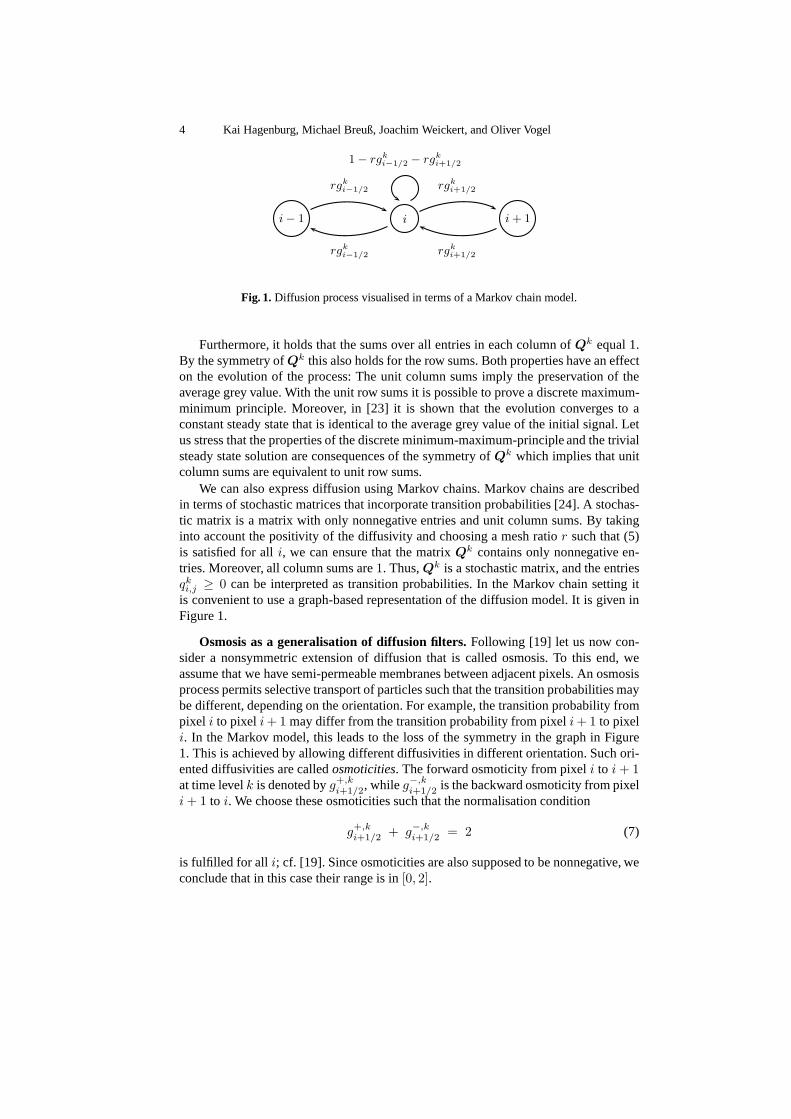
Fig. 1. Diffusion process visualised in terms of a Markov chain model.

Furthermore, it holds that the sums over all entries in each column ofQk equal 1.By the symmetry ofQk this also holds for the row sums. Both properties have an effecton the evolution of the process: The unit column sums imply the preservation of theaverage grey value. With the unit row sums it is possible to prove a discrete maximum-minimum principle. Moreover, in [23] it is shown that the evolution converges to aconstant steady state that is identical to the average grey value of the initial signal. Letus stress that the properties of the discrete minimum-maximum-principle and the trivialsteady state solution are consequences of the symmetry ofQk which implies that unitcolumn sums are equivalent to unit row sums.

We can also express diffusion using Markov chains. Markov chains are describedin terms of stochastic matrices that incorporate transition probabilities [24]. A stochas-tic matrix is a matrix with only nonnegative entries and unitcolumn sums. By takinginto account the positivity of the diffusivity and choosinga mesh ratior such that (5)is satisfied for alli, we can ensure that the matrixQk contains only nonnegative en-tries. Moreover, all column sums are1. Thus,Qk is a stochastic matrix, and the entriesqki,j ≥ 0 can be interpreted as transition probabilities. In the Markov chain setting it

is convenient to use a graph-based representation of the diffusion model. It is given inFigure 1.

Osmosis as a generalisation of diffusion filters.Following [19] let us now con-sider a nonsymmetric extension of diffusion that is called osmosis. To this end, weassume that we have semi-permeable membranes between adjacent pixels. An osmosisprocess permits selective transport of particles such thatthe transition probabilities maybe different, depending on the orientation. For example, the transition probability frompixel i to pixel i+ 1 may differ from the transition probability from pixeli+ 1 to pixeli. In the Markov model, this leads to the loss of the symmetry inthe graph in Figure1. This is achieved by allowing different diffusivities in different orientation. Such ori-ented diffusivities are calledosmoticities. The forward osmoticity from pixeli to i+ 1at time levelk is denoted byg+,k

i+1/2, whileg−,ki+1/2 is the backward osmoticity from pixel

i+ 1 to i. We choose these osmoticities such that the normalisation condition

g+,ki+1/2 + g−,k

i+1/2 = 2 (7)

is fulfilled for all i; cf. [19]. Since osmoticities are also supposed to be nonnegative, weconclude that in this case their range is in[0, 2].

Novel Schemes for Hyperbolic PDEs Using Osmosis Filters from Visual Computing 5

i − 1 i i + 1

1 − rg−,ki−1/2

− rg+,ki+1/2

rg−,ki−1/2

rg+,ki−1/2

rg+,ki+1/2

rg−,ki+1/2

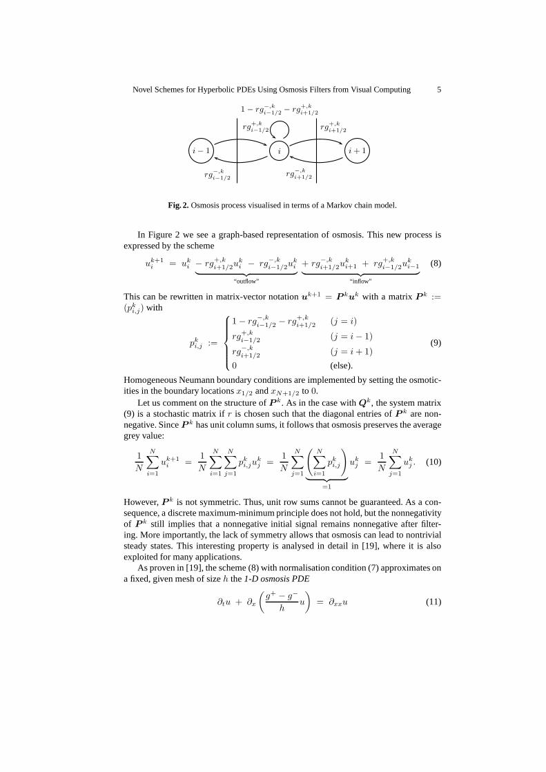
Fig. 2. Osmosis process visualised in terms of a Markov chain model.

In Figure 2 we see a graph-based representation of osmosis. This new process isexpressed by the scheme

uk+1i = uk

i − rg+,ki+1/2u

ki − rg−,k

i−1/2uki

︸ ︷︷ ︸

“outflow”

+ rg−,ki+1/2u

ki+1 + rg+,k

i−1/2uki−1

︸ ︷︷ ︸

“inflow”

(8)

This can be rewritten in matrix-vector notationuk+1 = P kuk with a matrixP k :=(pk

i,j) with

pki,j :=

1 − rg−,ki−1/2 − rg+,k

i+1/2 (j = i)

rg+,ki−1/2 (j = i− 1)

rg−,ki+1/2 (j = i+ 1)

0 (else).

(9)

Homogeneous Neumann boundary conditions are implemented by setting the osmotic-ities in the boundary locationsx1/2 andxN+1/2 to 0.

Let us comment on the structure ofP k. As in the case withQk, the system matrix(9) is a stochastic matrix ifr is chosen such that the diagonal entries ofP k are non-negative. SinceP k has unit column sums, it follows that osmosis preserves the averagegrey value:

1

N

N∑

i=1

uk+1i =

1

N

N∑

i=1

N∑

j=1

pki,ju

kj =

1

N

N∑

j=1

(N∑

i=1

pki,j

)

︸ ︷︷ ︸

=1

ukj =

1

N

N∑

j=1

ukj . (10)

However,P k is not symmetric. Thus, unit row sums cannot be guaranteed. As a con-sequence, a discrete maximum-minimum principle does not hold, but the nonnegativityof P k still implies that a nonnegative initial signal remains nonnegative after filter-ing. More importantly, the lack of symmetry allows that osmosis can lead to nontrivialsteady states. This interesting property is analysed in detail in [19], where it is alsoexploited for many applications.

As proven in [19], the scheme (8) with normalisation condition (7) approximates ona fixed, given mesh of sizeh the1-D osmosis PDE

∂tu + ∂x

(g+ − g−

hu

)

= ∂xxu (11)

6 Kai Hagenburg, Michael Breuß, Joachim Weickert, and Oliver Vogel

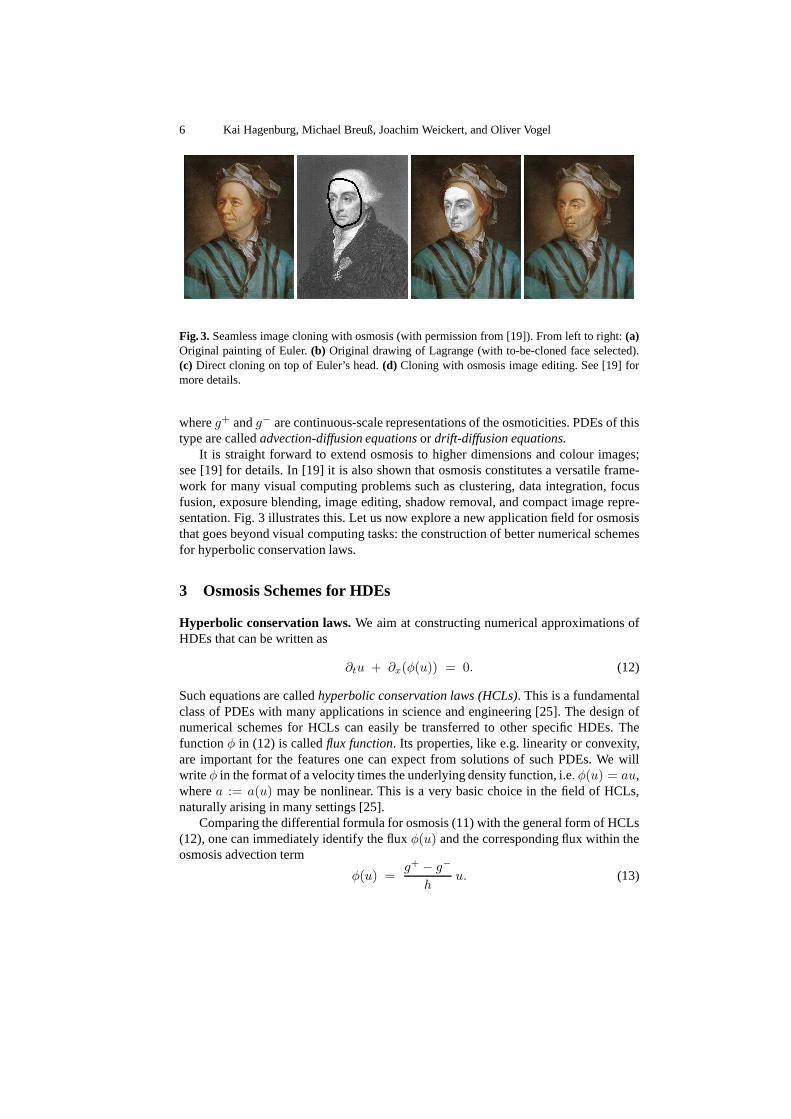
Fig. 3. Seamless image cloning with osmosis (with permission from [19]). From left to right:(a)Original painting of Euler.(b) Original drawing of Lagrange (with to-be-cloned face selected).(c) Direct cloning on top of Euler’s head.(d) Cloning with osmosis image editing. See [19] formore details.

whereg+ andg− are continuous-scale representations of the osmoticities. PDEs of thistype are calledadvection-diffusion equationsor drift-diffusion equations.

It is straight forward to extend osmosis to higher dimensions and colour images;see [19] for details. In [19] it is also shown that osmosis constitutes a versatile frame-work for many visual computing problems such as clustering,data integration, focusfusion, exposure blending, image editing, shadow removal,and compact image repre-sentation. Fig. 3 illustrates this. Let us now explore a new application field for osmosisthat goes beyond visual computing tasks: the construction of better numerical schemesfor hyperbolic conservation laws.

3 Osmosis Schemes for HDEs

Hyperbolic conservation laws.We aim at constructing numerical approximations ofHDEs that can be written as

∂tu + ∂x(φ(u)) = 0. (12)

Such equations are calledhyperbolic conservation laws (HCLs). This is a fundamentalclass of PDEs with many applications in science and engineering [25]. The design ofnumerical schemes for HCLs can easily be transferred to other specific HDEs. Thefunctionφ in (12) is calledflux function. Its properties, like e.g. linearity or convexity,are important for the features one can expect from solutionsof such PDEs. We willwriteφ in the format of a velocity times the underlying density function, i.e.φ(u) = au,wherea := a(u) may be nonlinear. This is a very basic choice in the field of HCLs,naturally arising in many settings [25].

Comparing the differential formula for osmosis (11) with the general form of HCLs(12), one can immediately identify the fluxφ(u) and the corresponding flux within theosmosis advection term

φ(u) =g+ − g−

hu. (13)

Novel Schemes for Hyperbolic PDEs Using Osmosis Filters from Visual Computing 7

In addition, there is the diffusion term∂xxu. The general idea we pursue in the followingis to determine useful expressions forg+ andg−, so that we can capture the hyperbolictransport by the osmosis model.

Selection of the osmoticities.For the general construction of osmosis-based algo-rithms, we stick for simplicity to the 1-D situation. The methodology can be extendedto the 2-D case in a straight forward fashion.

In order to approximate the fluxφ(u) = a(u)u of the hyperbolic transport containedin (11), we choose as osmoticities

g+,ki+1/2 := 1 +

h aki+1/2

2and g−,k

i+1/2 := 1 −h ak

i+1/2

2(14)

with velocitiesaki+1/2 defined at pixel borders. This setting makes the osmotic transport

identical to the desired formata(u)u. Let us discuss two examples.

– Example 1: Osmoticities for linear advection.The linear advection equation

∂tu + α ∂xu = 0 (15)

is a standard example of HDEs, defined viaφ(u) := αu with α ∈ R. In order toapproximate (15), we set all velocitiesak

i+1/2 to the same valueα.

– Example 2: Osmoticities for Burgers’ equation.Burgers’ equation is a classic test case for nonlinear HDEs:

∂tu + ∂x

(1

2u2

)

= 0, i.e. φ(u) =1

2u2. (16)

Rewriting the flux in the formatφ(u) = a(u)u leads to the discrete expression

aki+1/2 = a(uk

i , uki+1) :=

1

2

uki + uk

i+1

2(17)

after approximating the densityuki+1/2 at the border between pixelsi andi+ 1 by

averaging.

Subtracting the diffusion. Our osmosis scheme contains the diffusive term∂xxuwhich leads to an additional smoothing of the signal. In order to compensate for thiseffect, we apply a method similar to the fully discrete SID step in [17].

If we use our definitions ofg±i±1/2 from (14) within the osmosis filter (8) and carryout further computations, we obtain

uki = uk

i −τ

h

(

aki+1/2

uki+1 + uk

i

2− ak

i−1/2

uki + uk

i−1

2

)

︸ ︷︷ ︸

(A)

+ r (uki+1 − 2uk

i + uki−1)

︸ ︷︷ ︸

(B)

. (18)

8 Kai Hagenburg, Michael Breuß, Joachim Weickert, and Oliver Vogel

The term (A) corresponds to the update formula of an explicitscheme for discretisingthe hyperbolic transport, while (B) is a discretisation of atime step performed withlinear diffusion. It should be noted that (18) varies from the standard Lax-Friedrichsscheme by controlling the diffusive part (B) with the same time step sizeτ as the trans-port term (A), see also [25–27].

Let us now subtract the effect of the latter by performing a SID step in the samestyle as in [16, 17]. This gives the total, corrected result

uk+1i := uk

i − cki+1/2 + cki−1/2 (19)

wherecki±1/2 denote the fluxes of the stabilised inverse diffusion:

cki+1/2 := minmod(

uki − uk

i−1, ηki+1/2

(uk

i+1 − uki

), uk

i+2 − uki+1

)

(20)

with the minmod function

minmod(a, b, c) :=

max(a, b, c) if a > 0 andb > 0 andc > 0min(a, b, c) if a < 0 andb < 0 andc < 00 else.

(21)

Thereby,ηki+1/2 := r is the antidiffusion coefficient, as identified in (B). The other

arguments of the minmod function serve as stabilisers.

The complete algorithm.Now we can summarise our method in a nutshell.

Osmosis-based Method for Approximating∂tu+ ∂x(φ(u)) = 0.Step 1:Determine the velocity functiona for a given flux function

φ(u) = a(u)u.Step 2:Compute the osmoticities according to (14).Step 3:Perform one predictor step by applying the osmosis scheme (18).Step 4:Perform the corrector step (19).Step 5:Repeat steps 2 to 4 until the stopping time is reached.

4 Numerical Experiments

We illustrate the quality of our osmosis-based algorithm with several standard examplesfrom the field of HDEs. Thereby, we focus our attention on the shocks that are the mostinteresting features of hyperbolic PDEs.

For comparison with standard methods for HDEs, we employ a second-order high-resolution MUSCL-Hancock method [21, 22]. This classic method gives typical resultsfor high-resolution solvers in this field.

Linear advection in 1D. In our first experiment we consider the linear advectionequation (15) withα = 1 and periodic boundary conditions. We apply it for transportinga box-like initial signal

f(x) :=

{1 (10 ≤ x < 30)0 (else).

(22)

Novel Schemes for Hyperbolic PDEs Using Osmosis Filters from Visual Computing 9

0

0.2

0.4

0.6

0.8

1

50 60 70 80 90 100 110

Linear Advection Experiment at t=100

MUSCL-Hancocknovel scheme

true solution

0

0.2

0.4

0.6

0.8

1

80 85 90 95 100

Linear Advection Experiment at t=100 (Close-up)

MUSCL-Hancocknovel scheme

true solution

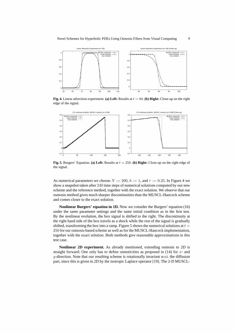
Fig. 4.Linear advection experiment.(a) Left: Results att = 60. (b) Right: Close-up on the rightedge of the signal.

-0.1

0

0.1

0.2

0.3

0.4

0.5

0.6

0 50 100 150 200

2-D nonlinear problem, MUSCL solution at t=1000

MUSCL-Hancocknovel scheme

true solution

-0.1

0

0.1

0.2

0.3

0.4

0.5

0.6

140 145 150 155 160

2-D nonlinear problem, MUSCL solution at t=1000 (Close-up)

MUSCL-Hancocknovel scheme

true solution

Fig. 5. Burgers’ Equation.(a) Left: Results att = 250. (b) Right: Close-up on the right edge ofthe signal.

As numerical parameters we chooseN := 200, h := 1, andτ := 0.25. In Figure 4 weshow a snapshot taken after240 time steps of numerical solutions computed by our newscheme and the reference method, together with the exact solution. We observe that ourosmosis method gives much sharper discontinuities than theMUSCL-Hancock schemeand comes closer to the exact solution.

Nonlinear Burgers’ equation in 1D. Now we consider the Burgers’ equation (16)under the same parameter settings and the same initial condition as in the first test.By the nonlinear evolution, the box signal is shifted to the right. The discontinuity atthe right hand side of the box travels as a shock while the restof the signal is graduallyshifted, transforming the box into a ramp. Figure 5 shows thenumerical solutions att =250 for our osmosis-based scheme as well as for the MUSCL-Hancock implementation,together with the exact solution. Both methods give reasonable approximations in thistest case.

Nonlinear 2D experiment. As already mentioned, extending osmosis to 2D isstraight forward: One only has to define osmoticities as proposed in (14) forx- andy-direction. Note that our resulting scheme is rotationallyinvariant w.r.t. the diffusionpart, since this is given in 2D by the isotropic Laplace operator [19]. The 2-D MUSCL-

10 Kai Hagenburg, Michael Breuß, Joachim Weickert, and Oliver Vogel

0 10 20 30 40 50 60 70 80 90 100 0 10

20 30

40 50

60 70

80 90

100

-1

-0.5

0

0.5

1

1.5

2-D nonlinear problem, MUSCL solution at t=250

-1.5

-1

-0.5

0

0.5

1

1.5

2

0 10 20 30 40 50 60 70 80 90 100 0 10

20 30

40 50

60 70

80 90

100

-1

-0.5

0

0.5

1

1.5

2-D nonlinear problem, novel scheme solution at t=250

-1.5

-1

-0.5

0

0.5

1

1.5

2

0 10 20 30 40 50 60 70 80 90 100

0 10

20 30

40 50

60 70

80 90 100

-1

-0.5

0

0.5

1

1.5

2-D nonlinear problem, MUSCL solution at t=250

-1.5

-1

-0.5

0

0.5

1

1.5

2

0 10 20 30 40 50 60 70 80 90 100

0 10

20 30

40 50

60 70

80 90 100

-1

-0.5

0

0.5

1

1.5

2-D nonlinear problem, novel scheme solution at t=250

-1.5

-1

-0.5

0

0.5

1

1.5

2

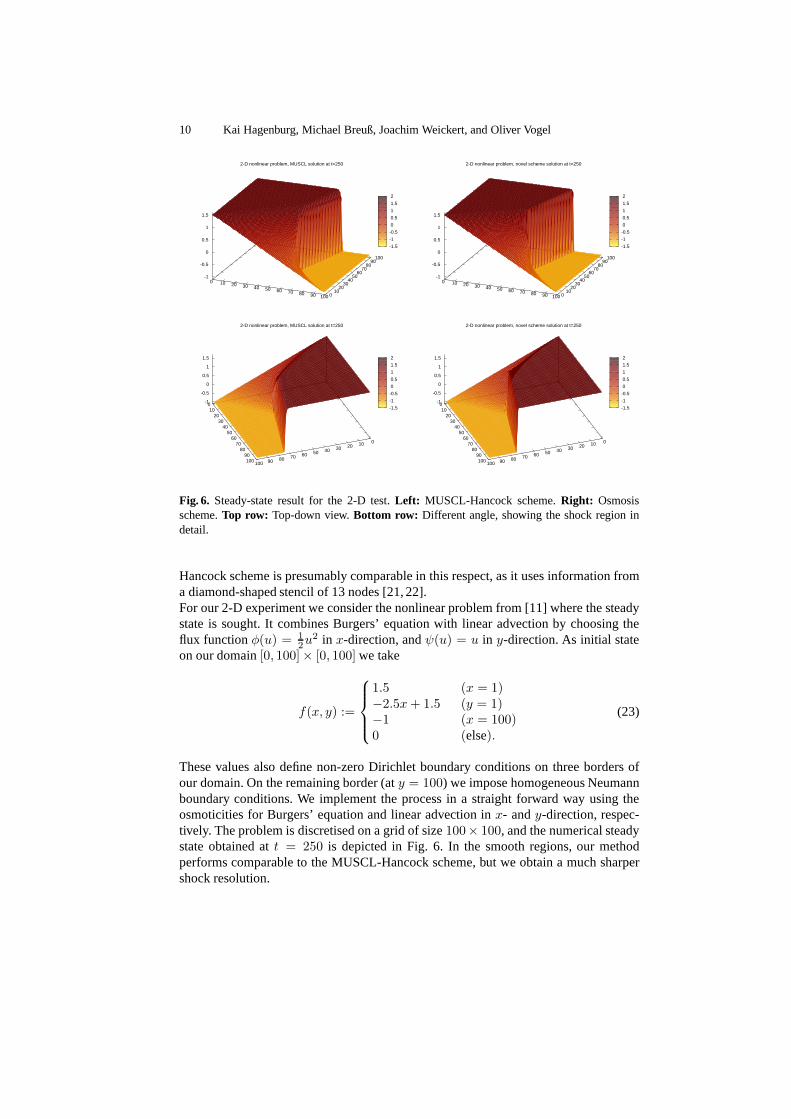
Fig. 6. Steady-state result for the 2-D test.Left: MUSCL-Hancock scheme.Right: Osmosisscheme.Top row: Top-down view.Bottom row: Different angle, showing the shock region indetail.

Hancock scheme is presumably comparable in this respect, asit uses information froma diamond-shaped stencil of 13 nodes [21, 22].For our 2-D experiment we consider the nonlinear problem from [11] where the steadystate is sought. It combines Burgers’ equation with linear advection by choosing theflux functionφ(u) = 1

2u2 in x-direction, andψ(u) = u in y-direction. As initial state

on our domain[0, 100]× [0, 100] we take

f(x, y) :=

1.5 (x = 1)−2.5x+ 1.5 (y = 1)−1 (x = 100)0 (else).

(23)

These values also define non-zero Dirichlet boundary conditions on three borders ofour domain. On the remaining border (aty = 100) we impose homogeneous Neumannboundary conditions. We implement the process in a straightforward way using theosmoticities for Burgers’ equation and linear advection inx- andy-direction, respec-tively. The problem is discretised on a grid of size100× 100, and the numerical steadystate obtained att = 250 is depicted in Fig. 6. In the smooth regions, our methodperforms comparable to the MUSCL-Hancock scheme, but we obtain a much sharpershock resolution.

Novel Schemes for Hyperbolic PDEs Using Osmosis Filters from Visual Computing 11

5 Conclusion

We have developed a novel class of schemes for approximatingHCLs. They combinerecently developed osmosis filters for resolving transportwith a stabilised inverse dif-fusion step. We have shown the strength of our approach for resolving solutions withshocks, which are important features in the fields of hyperbolic differential equations.

Quite frequently, new results in visual computing benefit from the use of moderntechniques from numerical analysis. Our work is an example for a fertilisation in theinverse direction. Note that the key for obtaining the results in our paper is the use of avery recent technique from visual computing. However, we donot only propose a novelconstruction of numerical schemes for HDEs, we also introduce a new application ofosmosis filters. Therefore, this paper is an example for the useful interaction of visualcomputing ideas and numerical analysis. In our future work we will investigate if alsoother modern PDE-based methods from image analysis can be used with benefit innumerical analysis.

Acknowledgments. The authors gratefully acknowledge the funding given by theDeutsche Forschungsgemeinschaft(DFG), grant We2602/8-1.

References

1. Rudin, L.I.: Images, Numerical Analysis of Singularities and Shock Filters. PhD thesis,California Institute of Technology, Pasadena, CA (1987)

2. Osher, S., Rudin, L.I.: Feature-oriented image enhancement using shock filters. SIAMJournal on Numerical Analysis27 (1990) 919–940

3. Alvarez, L., Mazorra, L.: Signal and image restoration using shock filters and anisotropicdiffusion. SIAM Journal on Numerical Analysis31 (1994) 590–605

4. Kornprobst, P., Deriche, R., Aubert, G.: Image coupling,restoration and enhancement viaPDEs. In: Proc. 1997 IEEE International Conference on ImageProcessing. Volume 4., Wash-ington, DC (October 1997) 458–461

5. Osher, S., Rudin, L.: Shocks and other nonlinear filteringapplied to image processing. InTescher, A.G., ed.: Applications of Digital Image Processing XIV. Volume 1567 of Proceed-ings of SPIE. SPIE Press, Bellingham (1991) 414–431

6. Breuß, M., Welk, M.: Analysis of staircasing in semidiscrete stabilised inverse linear diffu-sion algorithms. Journal of Computational and Applied Mathematics206(2007) 520–533

7. Pollak, I., Willsky, A.S., Krim, H.: Image segmentation and edge enhancement with stabi-lized inverse diffusion equations. IEEE Transactions on Image Processing9(2) (February2000) 256–266

8. Gilboa, G., Sochen, N.A., Zeevi, Y.Y.: Forward-and-backward diffusion processes for adap-tive image enhancement and denoising. IEEE Transactions onImage Processing11(7)(2002) 689–703

9. Welk, M., Gilboa, G., Weickert, J.: Theoretical foundations for discrete forward-and-backward diffusion filtering. In Tai, X.C., Mørken, K., Lysaker, M., Lie, K.A., eds.: Scale-Space and Variational Methods in Computer Vision. Volume 5567 of Lecture Notes in Com-puter Science. Springer, Berlin (2009) 527–538

10. Breuß, M., Zimmer, H., Weickert, J.: Can variational models for correspondence problemsbenefit from upwind discretisations? Journal of Mathematical Imaging and Vision39(5)(2011) 230–244

12 Kai Hagenburg, Michael Breuß, Joachim Weickert, and Oliver Vogel

11. Grahs, T., Meister, A., Sonar, T.: Image processing for numerical approximations of conser-vation laws: nonlinear anisotropic artificial dissipation. SIAM Journal on Scientific Comput-ing 23(5) (2002) 1439–1455

12. Grahs, T., Sonar, T.: Entropy-controlled artificial anisotropic diffusion for the numericalsolution of conservation laws based on algorithms from image processing. Journal of VisualCommunication and Image Representation13(1/2) (2002) 176–194

13. Wei, G.: Shock capturing by anisotropic diffusion oscillation reduction. Computer PhysicsCommunications144(2002) 317–342

14. Boris, J.P., Book, D.L.: Flux corrected transport. I. SHASTA, a fluid transport algorithm thatworks. Journal of Computational Physics11(1) (1973) 38–69

15. Burgeth, B., Pizarro, L., Breuß, M., Weickert, J.: Adaptive continuous-scale morphology formatrix fields. International Journal of Computer Vision92(2) (2011) 146–161

16. Breuß, M., Weickert, J.: A shock-capturing algorithm for the differential equations of dilationand erosion. Journal of Mathematical Imaging and Vision25 (2006) 187–201

17. Breuß, M., Weickert, J.: Highly accurate schemes for PDE-based morphology with generalstructuring elements. International Journal of Computer Vision92(2) (2011) 132–145

18. Breuß, M., Brox, T., Sonar, T., Weickert, J.: Stabilizednonlinear inverse diffusion for ap-proximating hyperbolic PDEs. In Kimmel, R., Sochen, N., Weickert, J., eds.: Scale-Spaceand PDE Methods in Computer Vision. Volume 3459 of Lecture Notes in Computer Science.,Berlin, Springer (2005) 536–547

19. Weickert, J., Hagenburg, K., Vogel, O., Breuß, M., Ochs,P.: Osmosis models for visualcomputing. Technical report, Department of Mathematics, Saarland University, Saarbrucken,Germany (2011)

20. LeVeque, R.J.: Numerical Methods for Conservation Laws. Birkhauser, Basel (1992)21. van Leer, B.: Towards the ultimate conservative difference scheme, V. A second order sequel

to Godunov’s method. Journal of Computational Physics32(1) (1979) 101–13622. Toro, E.F.: Riemann Solvers and Numerical Methods for Fluid Dynamics - A Practical

Introduction. 2nd edn. Springer, Berlin (1999)23. Weickert, J.: Anisotropic Diffusion in Image Processing. Teubner, Stuttgart (1998)24. Seneta, E.: Non-negative Matrices and Markov Chains. Springer Series in Statistics.

Springer, Berlin (1980)25. LeVeque, R.J.: Finite Volume Methods for Hyperbolic Problems. Cambridge University

Press, Cambridge, UK (2002)26. Breuß, M.: The correct use of the Lax-Friedrichs method.ESAIM: Mathematical Modeling

and Numerical Analysis38(3) (2004) 519–54027. Breuß, M.: An analysis of the influence of data extrema on some first and second order

central approximations of hyperbolic conservation laws. ESAIM: Mathematical Modelingand Numerical Analysis39(5) (2005) 965–993