1. Introduction Observing the current pace of economic activity is crucial to policy-makers and other
decision makers as it can affect, for example, the implementation of counter-cyclical
policies or near-term production decisions. However, the most important measure of
economic activity, GDP growth, is released with a two-month lag and is subject to
substantial revision. For this reason, policy-makers require reliable nowcasts (i.e.,
current-period estimates) of GDP growth in order to monitor economic conditions.
The literature on nowcasting has evolved rapidly in the last few years, although it has
a long history, beginning with the work of Mitchell and Burns (1938), who classified
hundreds of variables as leading, coincident or lagging indicators. This NBER-type
study on indicators was regularly updated for the next thirty years, but then waned
around the seventies. Stock and Watson (1989, 1991) subsequently renewed interest
in coincident indicators via the construction of simple indexes. More recent studies
(e.g. Nunes (2005), Camacho and Perez-Quiros (2008)) have focused on the
construction of models primarily for very short-term forecasting, while others (e.g.
Andreou, Ghysels and Kourtellos (2010)) have focused on methodological
contributions aimed at improving the incorporation of variables measured at
different frequencies within a single model. A related strand of literature aims at
constructing high-frequency indexes capable of capturing turning points in the
business cycle in a timely manner (e.g. Aruoba, Diebold and Scotti (2009)).
The main contribution of the present study is in investigating a broadening of the
information set at the disposal of nowcasters. We have compiled, and examine the
utility of, a database on the payments system in Canada, providing us with
information on the values and volumes of debit and credit card transactions, as well
as of cheques that clear through the banking system. Apart from providing new
proxies for household and business spending, these data have the benefit of being
compiled electronically, thereby being available on a timely basis, as well as being
virtually free of measurement error.
2
The data on debit and chequing transactions were constructed by aggregating the
various payments that clear through the members of the Canadian Payments
Association (CPA) on a daily basis. With the payments data being organized by
transactions between the different CPA members, and also by type of payment and
by region, each monthly observation on debit or chequing transactions that we
computed required aggregating the information in a 120,000-row spreadsheet.
Meanwhile, credit card transactions were obtained from the Canadian Bankers’
Association, which aggregates Visa and MasterCard transactions on a monthly basis.
Several previous studies have used electronic payments data on a limited basis,
usually within an empirical industrial organization context (e.g. Shankar and Bolton
2004), while others have used scanner data to understand price movements (e.g.
Silver and Heravi 2001, Burstein, Eichenbaum and Rebelo 2005). However, to our
knowledge, a study using such a broad range of payments data to nowcast GDP
growth has not been undertaken for any country.
Methodologically, this study follows Giannone, Reichlin and Small (2008) in that we
track GDP nowcast improvements over time. Specifically, we assess the marginal
contribution of payments data over a five-month span, which extends from the first
day of a quarter until the month of the data's eventual release. The prima facie
evidence suggests that payments data typically lower nowcast errors, but the degree
of reduction is variable and, in the small sample sizes inevitable in dealing with
quarterly GDP data, there is not sufficient power to obtain any statistically significant
reduction.
Nonetheless, it is noteworthy that even relatively small nowcast errors can generate
negative publicity for policy makers. For example, the following quotation appeared
in the financial press on Monday, June 4, 2012, following the release of 2012Q1 GDP
growth on Friday, June 1:
3
On Friday, we learned that the Canadian economy grew just 1.9 per cent
at an annual pace in the first quarter, making a mockery of the Bank of
Canada’s forecast of 2.5 per cent growth. Indeed, markets appear to be
enjoying a good chuckle at the expense of the Bank of Canada these
days. The yield on the Government of Canada 10-year bond fell below
1.62 per cent last week, marking its lowest level since at least 1950. The
threat of rate hikes usually sends bond yields higher, not lower.1
The context of the above quotation is that the Bank had begun hinting at a rate
increase with the release of its April Monetary Policy Report. Economic momentum
appeared to be picking up, given that it revised its forecast for 2012Q1 GDP growth
up to 2.5 per cent on 18 April, 2012, from 1.8 per cent, which had been its forecast
for 2012Q1 published on 18 January, 2012. Consequently, although the Bank
appeared to be preparing markets for rate increases, it later appeared that markets
were dictating that the policy rate should instead fall.
This recent example illustrates several points: (1) Policy credibility can be gained or
lost with nowcasts; (2) nowcasts can have an impact on expected policy decisions,
and thus bond yields; (3) nowcasts for a given quarter can evolve over time,
sometimes substantially; and (4) a lot of emphasis is placed on the accuracy of a
nowcast relative to the first release of GDP growth, even though it is well known that
GDP growth is subsequently revised.2
The present paper will track nowcasts produced at different points in time for a
given quarter, and demonstrate how nowcast performance varies with updated data,
and whether electronic payments can contribute to improving nowcast performance,
while taking into consideration revisions to monthly GDP growth.
1 Berman, D. (2012) “Rate Hikes? Rate Cuts More Likely.” The Globe and Mail, June 4, 2012.
2 We find that the mean absolute revision to annualized quarterly GDP growth in Canada from 2005 to 2009
is 0.63 percentage points, so the 0.60 percentage point deviation between the Bank’s nowcast and the initial
release for 2012Q1 could eventually simply be explained by a subsequent upward revision of GDP growth
by Statistics Canada.
4
In the next section we describe the payments data that, as we noted above, are being
used for the first time in this context, as well as the variables used in our base-case
model. In Section 3 we present the model used for our GDP nowcasting exercise,
which accounts for the release dates of our various indicators. In Section 4 we
conduct our nowcasting exercise on Canadian GDP growth, while Section 5
concludes.
2. Data
2.1 Payments Data
In the last fifteen years Canadians have increasingly adopted cashless means of
payment. They are among the world’s most intensive users of debit cards, with more
than 100 transactions per person per year, while credit cards account for about 25
percent of all transactions in the economy, roughly equivalent to the percentage of
transactions using cash. Although cheques account for less than 1% of all
transactions, the average value of small (under $50,000) cheques that clear through
the payments system is over $1,100, reflecting the fact that they are used for large
infrequent transactions, such as rent payments, tuition fees, income and property
taxes, or the purchase of big-ticket items such as automobiles.
These transactions are recorded, and the aggregated values are available rapidly.
The corresponding payments system variables, which we have compiled at a monthly
frequency from January 2000 through December 2009, are the following:
1. Debit: we capture point-of-sale (POS) payments that clear between two
institutions. This involves a debit from the consumer’s bank account and a
credit to the merchant’s account. This captures more than 80 percent of all
debit card transactions in the economy, with a national average of more than
100 transactions per second, 24 hours per day. We aggregate all debit
5
transactions for the members of the Canadian Payments Association (CPA),
who graciously provided the data. We have data on both the aggregate value
and volume of all debit transactions.
2. Credit: Visa and MasterCard dominate the Canadian credit card market,
accounting for about 90 percent of all credit card transactions in the economy.
These cards are issued by Canadian banks. We aggregate the monthly value of
all combined Visa and MasterCard transactions. These data were obtained
from the Canadian Bankers Association (CBA).
3. Cheques: as with debit cards, we capture all small cheques that clear between
banks. We choose to focus on cheques valued under $50,000, as these would
often be used for payments of goods and services, whereas larger-valued
cheques are typically used for financial transactions, which are less relevant
for an analysis of GDP movements. These data were obtained from the CPA.
As a general rule, debit cards are used for small- to medium-sized transactions, and
average about $48 per transaction; credit cards are typically used for larger
purchases, and average about $110; and cheques, while infrequently used, average
over $1,100. In Figure 1a we plot the average values of all three payment types from
2000 to 2009. We observe that each has regular seasonal peaks, and that cheques
and credit transactions tend to have a greater upward trend than average debit
transactions. Business-day payments system data are reported only for Monday
through Friday, excluding also public holidays. As a result, weekend and holiday
transactions must be recorded with the data of a weekday, typically but not
invariably Tuesday. In aggregating as we do to a monthly frequency, however, this
limitation is of no effect.
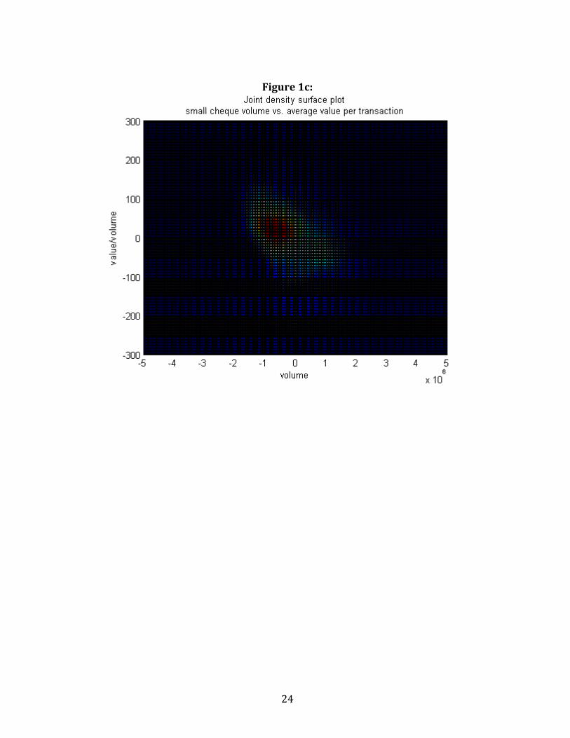
The CPA data record both value and volume of transactions for debit, small cheque
and large cheques. The ability to compare value and volume gives additional insight
into the interpretation of the data presented above; Figures 1b-1d describe the joint
distributions of volume and average value for each of the three means of payment.
6
Each of the Figures 1b-1d plots a joint density of volume of transactions per business
day, and average value per transaction (colour represents height according to the
usual convention; the density is estimated by kernel methods with bandwidth chosen
by cross-validation). The data plotted are residuals from a simple quadratic trend
model with a dummy variable for days on which aggregated weekend or holiday
transactions are reported.
The three means of payment display quite different patterns. For debit purchases,
higher volume of transactions is clearly associated with higher average value per
transaction; this may reflect larger volume and average value around holidays, for
example. For small cheques, there is some negative association, although there
appears to be little association in the most concentrated region. For large cheques,
there is very little association between average value and volume (most of the
probability mass is approximately parallel to the volume axis). Of course, the degree
of association between value and volume affects the potential value of including both
in a forecasting equation.
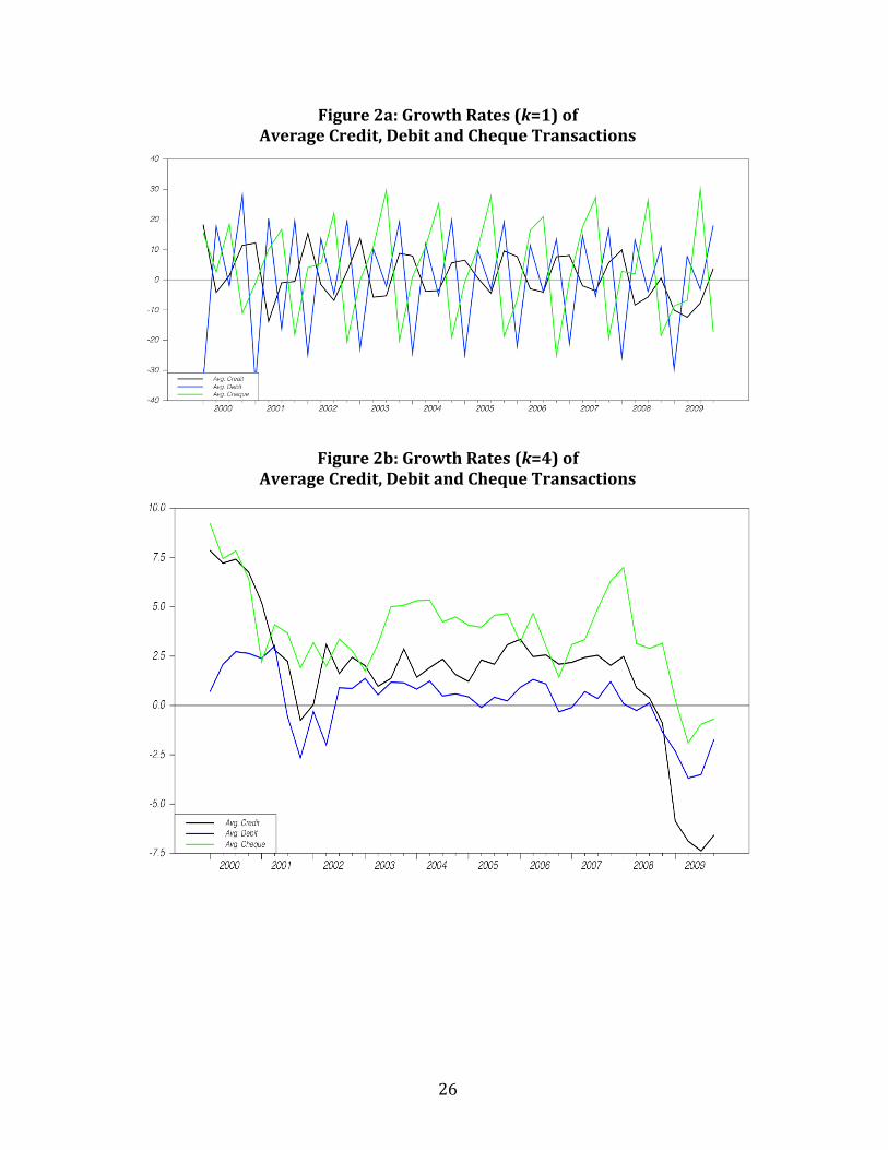
Since we are interested in nowcasting GDP growth, we will also have to study the
growth rates of these series. The annualized growth rate of any payments variable xt
is computed over k quarters as:
(1)
Ý x t logxt
xtk
400
k
In Figures 2a and 2b we plot, respectively, the quarter-over-quarter (k=1) and the
year-over-year (k =4) annualized growth rates of these three series. We plot both
since we are interested in both quarterly and annual GDP growth, and so will require
a different transformation of the payments variables for each growth rate studied.
Figure 2a reveals the strong seasonal patterns of these payments data. Interestingly,
the peaks and troughs of these data occur in different periods. Specifically, cheques
tend to peak in Q3, debit cards in Q4 and credit cards in Q4 or Q1. Although we make
7
no attempt in this paper to model the choice of payments instrument by consumers,
Galbraith and Tkacz (2013) found that daily debit card transactions accelerated in
both value and volume during the four weeks prior to Christmas; with bank accounts
depleted during the holidays, households may therefore increasingly rely on credit
cards while they rebuild their savings in Q1. Meanwhile, cheques may be peaking in
Q3 to reflect infrequent transactions that occur that quarter, such as property tax or
tuition payments. Regardless of the exact causes, having all three payments types at
our disposal allows us to control for any substitution effects between these payments
methods, thereby allowing us to isolate better the impact of these variables on GDP
growth. For example, a consumer choosing to switch to a credit card from a debit
card for grocery purchases would result in a growth in credit card transactions and a
fall in debit transactions. For this reason, using any series in isolation could lead to
false signals about economic activity, whereas using all of them in a model would
endogenize a consumer’s choice of payment technology, thereby providing better
signals about economic activity.
However, if households display “payments inertia” and infrequently switch between
payments methods, then having all payments methods in a model will not necessarily
produce better nowcasts, as some payments methods may display more sensitivity to
economic conditions than others. For instance, debit card transactions may fall more
rapidly than credit card transactions during a recession, as the former cannot be
used once savings are depleted, while the latter may still be used even if savings are
zero and one’s job has been lost. As a result, determining which to include in a model
is an empirical question, and so we will consider various payments methods
combinations in our nowcasting exercise.
The year-over-year growth rates (Figure 2b) are smoother, and reveal a clearer
picture of the business cycle. The recession of 2008-09 appears as sharp drops in all
three payments variables, while the slowdown in 2001Q3 (which met the technical
definition of a recession in the United States but was only a single quarter of negative
growth in Canada) is clearly visible, and also reveals a slowdown in the growth of
8
average payments. In that period, which includes the attacks of 9/11, we observe
that both average debit and credit transactions showed negative growth rates.
To control for seasonal effects, we seasonally adjust our payments data using the
X11-ARIMA process, which is the same used for adjusting GDP in the National
Accounts. In Section 4 we repeatedly seasonally adjust the payments data as we
update our sample through the out-of-sample nowcasting exercise in order to ensure
that we replicate the data that would have been available to analysts in the past.
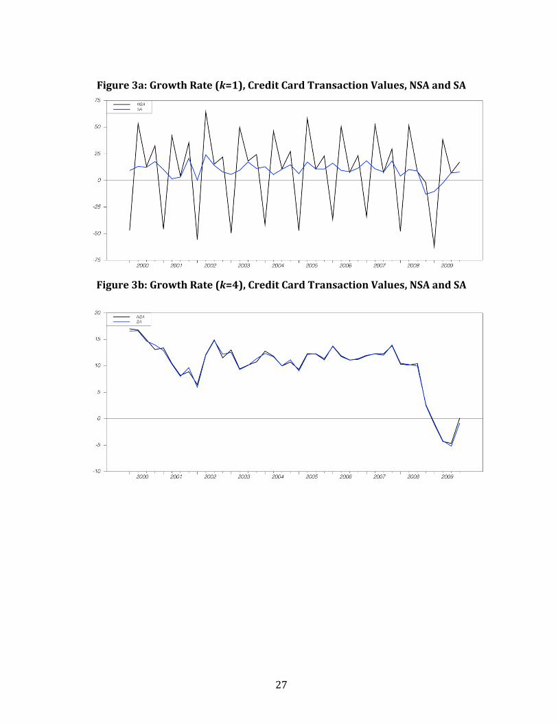
However, for exposition purposes we present in Figures 3a and 3b the non-
seasonally-adjusted (NSA) and seasonally-adjusted (SA) quarterly and year-over-
year growth rates of credit card values. In Figure 3a we observe that many of the
wide credit card fluctuations are largely due to seasonal factors, as the adjusted
series is much smoother. In Figure 3b the original series shows virtually no seasonal
features. This follows from the manner in which this series is constructed, as it
compares the level in the current quarter to that of the similar quarter one year
prior. In our empirical work we will be using the SA series for nowcasting both
quarterly and annual GDP growth, although for the latter case there is little
difference between SA and NSA data.
A notable payments technology absent from our list of payments methods is cash,
and this follows for two reasons. First, all our models incorporate the growth of
narrow money, which is one component of the Composite Leading Index, which we
use as a control variable and discuss further below. Second, cash is most often used
for “small” transactions, and so cash purchases would be least correlated with
aggregate spending fluctuations, which are most affected by consumer spending
decisions on larger discretionary items. According to Arango, Huynh and Sabetti
(2011), debit and credit cards account for about 89% of the value of retail
transactions above $50, while cash is used for the remaining 11%. Cash is most
widely used for transactions under $15, with 59% of the value of all such
transactions being made using cash. By contrast cheques are almost never used for
retail purchases in Canada, although as mentioned above they capture large,
9
infrequent payments that could crowd out discretionary purchases made using debit
and credit, and so are worth retaining for this purpose.
2.2 Basecase Indicators
Although a visual inspection of Figure 2b leads one to suspect that payments
variables are correlated with the business cycle, more careful scrutiny suggests that
we need to assess the information content of these variables relative to indicators
that are already regularly compiled and monitored. In other words, we need to
assess whether they provide any new information at the margin.
Apart from lagged GDP growth, we experimented with several candidate variables3
that could be useful for nowcasting, but only one was retained, as it helped achieve
the lowest nowcast errors, was available on a timely basis, and already captures
movements in several other variables. The Composite Leading Index (CLI), is
constructed by Statistics Canada as a simple average of ten different variables that
capture movements in the business cycle from various sectors, and standardized
such that its mean and standard deviation correspond to that of GDP growth. The ten
variables that comprise the CLI are:
Group 1: Leading Indicators
Housing index (housing starts and MLS housing sales)
Business and personal services employment
TSX stock index
Narrow money supply (real)
U.S. CLI
Group 2: Manufacturing
Average work week (hours)
3 We considered the unemployment rate, various interest rates and interest rate spreads, stock prices, and the
exchange rate. Many of these variables proved useful for longer-term forecasts, but were not as useful for
nowcasting purposes.
10
New orders, durables
Shipments/inventories of finished goods
Group 3: Retail Trade
Furniture and appliance sales
Other durable goods sales
Once all the data are compiled, the CLI for a given month t is released around the
third week of month t+1.
The key benefits of the CLI are that (1) this variable captures movements in a broad
range of sectors in a single number; and (2) it is released in a relatively timely
manner. However, within the CLI some of the components are measured with a lag,
as they rely on survey data. This is the case for the Retail Trade variables, as well as
new orders of durables and shipments/inventories of finished goods in the
Manufacturing group; for the CLI of a given month t, data for these components
actually reflect observations for month t-2. In addition, the U.S. CLI would reflect
month t-1.
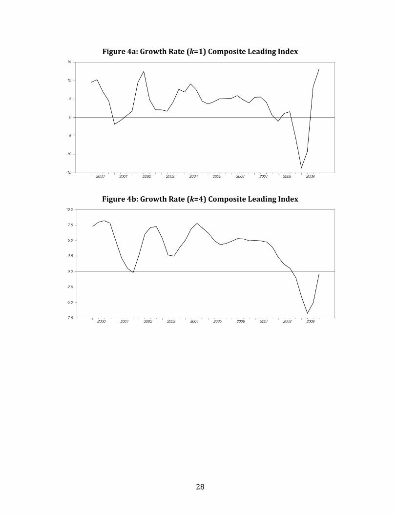
When using the CLI in our nowcasting equations we convert it to either quarterly or
year-over-year growth rates and plot these growth rates in Figures 4a and 4b. We
observe that the CLI also tends to follow a pattern that would correspond to the
business cycle of the last ten years, picking up in particular the recession of 2008-09
and the slowdown of 2001.
The remainder of this study is concerned with studying whether payments variables
add any relevant information that is not already captured by the CLI and lagged GDP
growth. However, to make fair comparisons we need to ensure that the relevant base
case model only incorporates information available at the time a nowcast is made. As
new information accrues over time, the models would then incorporate the new data,
and presumably the nowcasts would be converging to the “true” GDP growth rate. In
11
the next section we explain how we account for revisions to GDP growth, update our
models over time, and what data are available at each point in time.
2.3 Monthly GDP Growth
Our interest lies in nowcasting quarterly GDP growth, as this is the headline number
around which major policy decisions and announcements are made. For example, the
Bank of Canada’s Fixed Announcement Dates (FADs) are timed such that policy rate
decisions take into account recent GDP numbers. The quarterly release also reflects
complete updates to the income and expenditure accounts as GDP components are
updated at this time as well.
In between the quarterly National Accounts, Statistics Canada also releases estimates
of GDP by industry on a monthly basis, so this is a variable that can serve as an
important input into any quarterly nowcast. The quarterly number is simply an
average of the monthly numbers, so having knowledge of the growth rates of the first
two months of a quarter implies that two-thirds of a quarter is already known.
However, the monthly numbers are only released two months after the end of a given
month, so care must be taken when performing the GDP nowcasting exercise to
ensure that one uses only GDP observations that are actually available.
Apart from timeliness, as with quarterly GDP growth, the monthly observations are
also subject to revision. Tkacz (2010) found that year-over-year GDP growth in
Canada was revised on average by 0.25 percentage points. This number is not overly
large by international standards, but it is also not negligible. As a result, when using
monthly GDP to nowcast quarterly GDP it is important to use the vintage that would
have been available at the time a nowcast would have been produced.
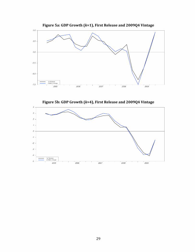
No public sources of real-time monthly Canadian GDP exist, so we constructed our
own using historical issues of Statistics Canada publications (Catalogue Number 15-
001X). In Figures 5a and 5b we plot the first and “final” (i.e. the 2009Q4) vintages of
12
quarterly and annual GDP growth rates. From Figure 5a we observe that revisions
tend to make peaks higher and troughs deeper, with the trough of the recession in
2009Q1 being revised down by almost a full percentage point. Note that the first-
release and “final” observations are the same in 2009Q4, since the first release of the
2009Q4 vintage was of course not yet revised at that time. In our out-of-sample
forecast horizon (2005 to 2009), the mean absolute revision for quarterly GDP
growth between the first-release and the 2009Q4 GDP vintage is 0.63 percentage
points, while for year-over-year GDP growth it is 0.23 percentage points.
Given the disparities between the first and final releases, we can compute GDP
nowcast errors for either of these two series, as there would be some interest in
both. However, we expect nowcasts to be more accurate for the first-release data, as
nowcasts would be conditional on first-release data. Furthermore policy decisions
are often based, and credibility gauged, on recently released data. For this reason our
RMSEs will be computed using the first-release data as the series to be nowcast. In
the Appendix we present some analogous results in which the final release of GDP is
the variable to be nowcast.
3. Nowcasting Equations and the Timing of Data Releases
From the discussion in Section 2, we can write
(2)
y f (lagged y,CLI,PAY)
where y is output growth; CLI the growth rate of the Composite Leading Index; PAY is
a vector of payments variables, which may include the value and volume of debit,
credit and chequing transactions.
The functional relationship may take various forms. We consider models that
aggregate information from the various predictors via OLS regression, model
13
averaging methods which combine results from numerous models having different
regressors (Hansen 2007), and dimension reduction methods which use principal
components of a regressor matrix and compare all information sets on a common
number of regressors (see Galbraith and Hodgson 2012 for an exposition of the latter
two classes of method). Because the results from the different methods were
qualitatively similar, we report here only the simplest least-squares forecast results.
Growth rates are computed as quarter-over-quarter or year-over-year, and we
present results for each case. Our “base case” model omits the payments variables;
we then consider five alternative models which respectively contain (i) the growth
rates of the value and volume of debit card transactions; (ii) the growth rates of the
value and volume of credit card transactions; (iii) the growth rates of the value and
volume of cheque transactions; (iv) the growth rates of the value and volume of debit
and credit transactions; and (v) the growth rates of the values and volumes of debit
cards, credit cards and cheques.
We have omitted from (2) time subscripts, as these would vary according to the
precise time at which an analyst would be required to generate a nowcast. However,
for estimation and nowcasting purposes we need to specify the appropriate datings.
In what follows we assume that one is required to generate a nowcast of GDP growth
for quarter t. The first nowcast is generated on the first day of the quarter, and a new
nowcast is generated on the first day of each subsequent month until the official
growth rate is released, which would be at the end of the second month of quarter
t+1.
For example, the third quarter of a year occurs in the months of July, August and
September, and the actual growth rate for Q3 would be released around November
30. Thus, an analyst would produce a nowcast for Q3 on July 1st, August 1st,
September 1st, October 1st and November 1st, for a total of five nowcasts. We would
expect that as time passes and new data become available, the nowcast will become
more precise as its production date is closer to the actual release date. With five
14
different nowcast production dates, and with new monthly data becoming available
for each one, the time subscripts on the explanatory variables in (2) would vary for
each production point within the quarter.
The release dates for GDP and the CLI are regular and known in advance. GDP is
always released two months after a given month, and the CLI around the third week
after a given month.
Since payments data are recorded electronically, they are in principle available at a
daily frequency, and released the next business day. For example, the Interac
Organization studies daily movements in debit card transactions, and regularly
compares year-over-year growth rates for transactions on specific days. Galbraith
and Tkacz (2013) in fact use daily debit transactions to assess the impact of extreme
events, such as 9/11 and the SARS pandemic, on economic activity. Similarly, credit
card companies precisely track their daily transactions, and often issue press
releases in the days leading up to Christmas to pinpoint the busiest transaction day
of the year. For this reason, should the demand exist, payments data for a given
month t can be available on the first day of month t+1, making these data extremely
timely relative to other spending indicators.
Given the release dates above, we can specify the five variants of (2) that an analyst
can estimate for each of the five different nowcasting points for a given quarter t.
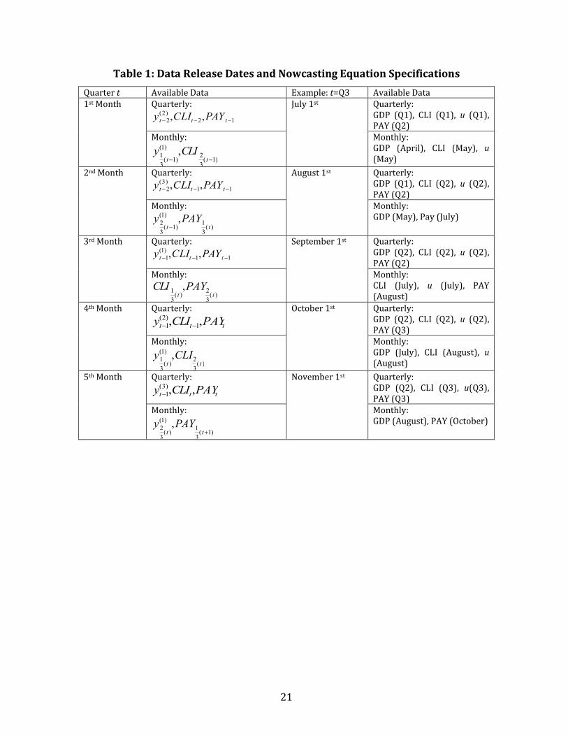
These time subscript specifications are provided in Table 1, and to facilitate the
discussion we provide an illustration using t=Q3. Superscripts denote the particular
vintage of GDP growth that is known at each point in time.
In each case we use whatever quarterly data is available. The monthly data is
incorporated into the nowcast by using the available monthly data to compute
average observations for the incomplete quarter. For example, when a nowcast is
generated on July 1st, an analyst would have CLI data for May. The growth rate of
these variables for April and May relative to January and February (i.e the first two
15
months of Q1) is used as a proxy growth rate for these variables for Q2. The more
data available for a quarter, the closer our estimate of the final value for that quarter,
and therefore the more accurate our nowcast.
4. Nowcasting Canadian GDP Growth
Our full sample begins in 2000Q1 and ends in 2009Q4, for a total of 40 quarterly
observations. In our nowcasting exercise we use the first 20 observations for initial
estimation of parameters, which are then used to produce a nowcast for 2005Q1. The
sample is updated by one quarter, parameters are re-estimated and a nowcast
produced for 2005Q2. This process is repeated until we obtain nowcasts for 2009Q4.
Given the different time subscripts associated with the variables in Table 1, we treat
each of the five specifications as a different model, and so we track the nowcasting
performance of each specification over the full nowcasting sample. For example, for
the specification in which a nowcast is produced during the first month of each
quarter, we track the accuracy of nowcasts produced on January 1st, April 1st, July 1st
and October 1st i.e. the first month of each quarter. The next specification uses the
data available at the beginning of the second month, and so a new set of nowcasts is
produced on February 1st, May 1st, August 1st and November 1st. We repeat this for
each of the five periods for which a nowcast for quarter t is required, as discussed in
Section 3.
In Figures 6a and 6b we plot the nowcasts of quarterly and year-over-year GDP
growth using the basecase model (i.e. without the payments variables), using the
data available at the beginning of each month. We can visually observe that the
nowcasts produced at the beginning of the quarter (i.e. the 1st month) are the least
accurate. Notably, they miss many of the turning points in GDP growth, and miss the
timing of the recession that began in 2008Q4. However, as more data become
available during the quarter, we see that the nowcasts approach actual GDP growth.
By the 5th month a nowcast for GDP growth is produced with knowledge of the
16
growth rates for the first two months of the quarter, so it is easier to nowcast the full
quarter.
Interestingly, it appears that by around the fourth nowcast of the quarter analysts
should be able to predict the turning points in GDP growth. For example, the trough
in GDP growth was accurately captured as 2009Q1, so by July 2009 (the fourth
month of 2009Q2), analysts should have been predicting an improvement in
economic activity using the basecase model. Meanwhile, the nowcasts produced in
the first two months do not appear to capture many turning points; only when lagged
quarterly GDP growth appears in the information set (month 3) does some ability to
pick up turning points appear.
In Figures 7a and 7b we plot a new set of nowcasts generated by the model
augmenteded with debit card transactions (both values and volumes). As with
Figures 6a and 6b we notice the improvements in nowcasting accuracy that accrue
over time, with those generated in the 1st month being least accurate, and those
generated in the 5th month being most accurate. However, it is not clear by visually
comparing Figures 6 and 7 whether the payments variables contribute to lowering
nowcast errors in a substantial manner. For this purpose we can study the root
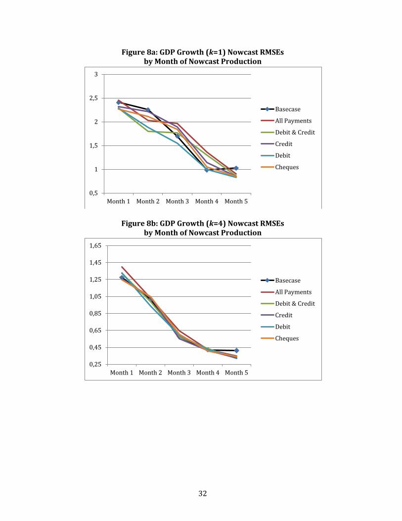
mean squared (nowcast) errors (RMSEs), which are presented in Figures 8a and 8b.
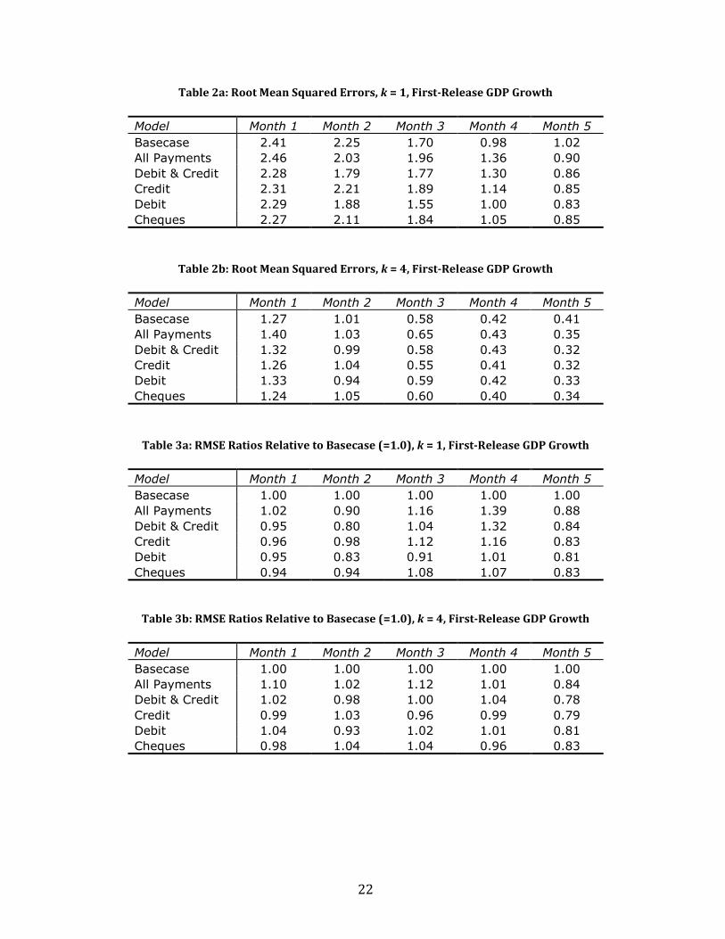
These graphs plot the RMSEs produced by the six different specifications at five
different points in time. As previously discussed, we assume that the series we are
attempting to nowcast accurately is the first release of GDP growth; results using the
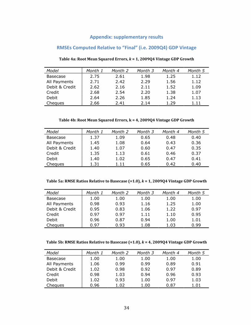
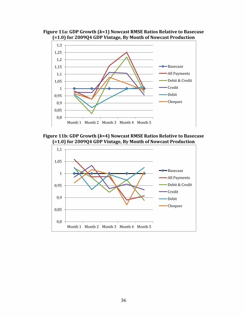
final GDP vintage may be found in the Appendix.
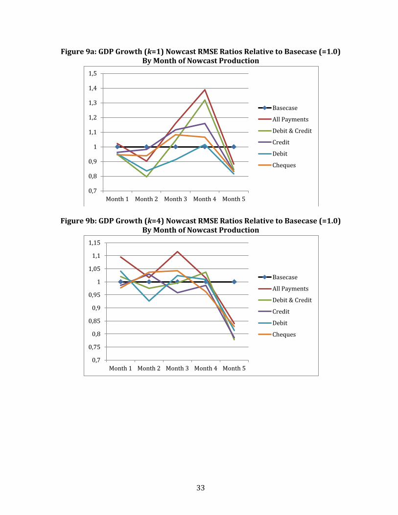
The base case RMSEs are denoted in black, with a diamond denoting the precise
values. Series below this line show improvements in nowcast accuracy. We see that
the base case RMSE drops from about 2.5 at month 1 to 1.0 in months 4 and 5. The
largest marginal improvements occur between Months 2 and 3 (when lagged
17
quarterly GDP growth first enters the information set) and Months 3 and 4 (when the
first monthly GDP observation for the quarter being nowcast is observed).
Payments variables tend show lower RMSE for the first two months, and also at
month 5. These improvements can be more clearly seen in Figures 9a and 9b. Largest
improvements involve lowering the RMSE by at most 20 per cent, and for quarterly
GDP growth this is achieved with the presence of debit card transactions in the
model. For the year-over-year growth rate, the largest improvement occurs at month
5, i.e. notable improvements in accuracy occur in the month immediately preceding
the release of the observation being nowcast.
It is the nature of GDP forecasting, or nowcasting, that there are few observations,
implying little statistical power to discriminate among rival models. Here, the out-of-
sample period includes only 20 observations.4 It is not possible to establish that any
of the point differences are statistically significant. However, given that this sample
contains the sharpest quarterly drop in economic activity ever observed in Canada,
the observed improvements in nowcasting accuracy do suggest the possibility that
payments variables could be of use in detecting downturns more rapidly.
5. Conclusion
Nowcasts matter for many decision-makers, and the present study documents the
degree to which the accuracy of nowcasts varies with the amount of information
available to an analyst: in these data the average nowcast error is approximately 60
per cent lower if produced just prior to a data release (month 5) compared with one
produced at the beginning of a quarter (month 1).
We assess how electronic payments, which are available on a timely basis, can
contribute to producing nowcasts. We find some evidence of improvement in
4 A forecast-encompassing test for nested models with data subject to revision, such as that of Clark and
McCracken (2009), could be performed, but results are unlikely to be statistically significant for such a
small sample.
18
nowcast accuracy when payments variables, particularly debit card payments, are
included in a model, especially when nowcasts are produced early or late in a
quarter. This suggests that the marginal contributions of such variables vary over a
quarter: they contain different amounts of information relative to other publicly
available data, at different points in time.
A desirable further development of this research would be to combine electronic
transactions with other data that can be measured with some accuracy at a daily
frequency, and a framework can be established that would automate the generation
of nowcasts on a daily basis as new data is observed. In this context we can also find
more effective methods for combining data at different frequencies within a single
model. The state space approach used by Armah (2011) could be one avenue worth
pursuing, as could a MIDAS mixed-frequency regression approach (e.g. Andreou,
Ghysels and Kourtellos (2010)).
19
References Andreou, E., E. Ghysels and A. Kourtellos (2010) “Regression Models with Mixed Sampling Frequencies.” Journal of Econometrics 158, 246-261. Arango, C., K. Huynh and L. Sabetti (2011) “How Do You Pay? The Role of Incentives at the Point-of-Sale.” Working Paper 2011-23, Bank of Canada. Armah, N. (2011) “Predictive Densities and State Space Nowcasting.” Working Paper, Bank of Canada. Aruoba, S. B., F. X. Diebold and C. Scotti (2009) “Real-Time Measurement of Business Conditions.” Journal of Business and Economic Statistics 27, 417-427. Burstein, A., M. Eichenbaum, and S. Rebelo (2005) “Large Devaluations and the Real Exchange Rate.” Journal of Political Economy 113, 742-784. Camacho, M. and G. Perez-Quiros (2008) “Introducing the Euro-STING: Short-Term Indicator of Euro-Area Growth.” Working Paper, Bank of Spain. Clark, T.E. and M.W. McCracken (2009) “Tests of Equal Predictive Ability with Real-Time Data.” Journal of Business and Economic Statistics 27, 441-454. Galbraith, J.W. and D. Hodgson (2012) “Dimension reduction and model averaging for estimation of artists' age-valuation profiles.” European Economic Review 56, 422-435. Galbraith, J. W. and G. Tkacz (2013) “Analyzing Economic Effects of September 11 and Other Extreme Events using Debit and Payments System Data.” Canadian Public Policy 39, 119-134. Giannone, D., L. Reichlin and D. Small (2008) “Nowcasting: The Real-Time Informational Content of Macroeconomic Data.” Journal of Monetary Economics 55, 665-676. Hansen, B. (2007) “Least squares model averaging.” Econometrica 75, 1175-1189. Mitchell, W. C. and A. F. Burns (1938) “Statistical Indicators of Cyclical Revivals.” In Moore, G. H. (Ed.) Business Cycle Indicators, Vol. 1. Princeton: Princeton University Press, 184-260, Reprinted 1961. Nunes, L. C. (2005) “Nowcasting Quarterly GDP Growth in a Monthly Coincident Indicator Model.” Journal of Forecasting 24, 575-592.
20
Shankar, V. and R. N. Bolton (2001) “An Empirical Analysis of Determinants of Retailer Pricing Strategy.” Marketing Science 23, 28-49. Silver, M. and S. Heravi (2001) “Scanner Data and the Measurement of Inflation.” The Economic Journal 111, F383-F404. Stock, J. and M. W. Watson (1989) “New Indexes of Coincident and Leading Economic Indicators.” NBER Macroeconomics Annual 1989, 351-394. Stock, J. and M. W. Watson (1991) “A Probability Model of the Coincident Economic Indicators.” In Leading Economic Indicators: New Approaches and Forecasting Records, Lahiri, K. and Moore, G.H. (eds) Cambridge: Cambridge University Press, 63-85. Tkacz, G. (2010) “An Uncertain Past: Data Revisions and Monetary Policy in Canada.” Bank of Canada Review, Spring, 41-51.
21
Table 1: Data Release Dates and Nowcasting Equation Specifications
Quarter t Available Data Example: t=Q3 Available Data 1st Month Quarterly:
y t 2
(2) ,CLIt2,PAY t1
July 1st Quarterly: GDP (Q1), CLI (Q1), u (Q1), PAY (Q2)
Monthly:
y1
3(t1)
(1) ,CLI 2
3(t1)
Monthly: GDP (April), CLI (May), u (May)
2nd Month Quarterly:
y t2
(3) ,CLIt1,PAY t1
August 1st Quarterly: GDP (Q1), CLI (Q2), u (Q2), PAY (Q2)
Monthly:
y 2
3(t1)
(1) ,PAY1
3( t )
Monthly: GDP (May), Pay (July)
3rd Month Quarterly:
y t1
(1) ,CLIt1,PAY t1
September 1st Quarterly: GDP (Q2), CLI (Q2), u (Q2), PAY (Q2)
Monthly:
CLI 1
3(t )
,PAY2
3(t )
Monthly: CLI (July), u (July), PAY (August)
4th Month Quarterly:
yt1
(2),CLIt1,PAYt
October 1st Quarterly: GDP (Q2), CLI (Q2), u (Q2), PAY (Q3)
Monthly:
y1
3(t )
(1) ,CLI2
3( t )
Monthly: GDP (July), CLI (August), u (August)
5th Month Quarterly:
yt1
(3),CLIt,PAYt
November 1st Quarterly: GDP (Q2), CLI (Q3), u(Q3), PAY (Q3)
Monthly:
y 2
3(t )
(1) ,PAY1
3( t1)
Monthly: GDP (August), PAY (October)
22
Table 2a: Root Mean Squared Errors, k = 1, First-Release GDP Growth
Model Month 1 Month 2 Month 3 Month 4 Month 5
Basecase 2.41 2.25 1.70 0.98 1.02
All Payments 2.46 2.03 1.96 1.36 0.90
Debit & Credit 2.28 1.79 1.77 1.30 0.86
Credit 2.31 2.21 1.89 1.14 0.85
Debit 2.29 1.88 1.55 1.00 0.83
Cheques 2.27 2.11 1.84 1.05 0.85
Table 2b: Root Mean Squared Errors, k = 4, First-Release GDP Growth
Model Month 1 Month 2 Month 3 Month 4 Month 5
Basecase 1.27 1.01 0.58 0.42 0.41
All Payments 1.40 1.03 0.65 0.43 0.35
Debit & Credit 1.32 0.99 0.58 0.43 0.32
Credit 1.26 1.04 0.55 0.41 0.32
Debit 1.33 0.94 0.59 0.42 0.33
Cheques 1.24 1.05 0.60 0.40 0.34
Table 3a: RMSE Ratios Relative to Basecase (=1.0), k = 1, First-Release GDP Growth
Model Month 1 Month 2 Month 3 Month 4 Month 5
Basecase 1.00 1.00 1.00 1.00 1.00
All Payments 1.02 0.90 1.16 1.39 0.88
Debit & Credit 0.95 0.80 1.04 1.32 0.84
Credit 0.96 0.98 1.12 1.16 0.83
Debit 0.95 0.83 0.91 1.01 0.81
Cheques 0.94 0.94 1.08 1.07 0.83
Table 3b: RMSE Ratios Relative to Basecase (=1.0), k = 4, First-Release GDP Growth
Model Month 1 Month 2 Month 3 Month 4 Month 5
Basecase 1.00 1.00 1.00 1.00 1.00
All Payments 1.10 1.02 1.12 1.01 0.84
Debit & Credit 1.02 0.98 1.00 1.04 0.78
Credit 0.99 1.03 0.96 0.99 0.79
Debit 1.04 0.93 1.02 1.01 0.81
Cheques 0.98 1.04 1.04 0.96 0.83
23
Figure 1a: Average Credit, Debit and Cheque Transactions ($) Credit and Debit: Left Scale; Cheque: Right Scale
Figure 1b:
24
Figure 1c:
25
Figure 1d:
26
Figure 2a: Growth Rates (k=1) of Average Credit, Debit and Cheque Transactions
Figure 2b: Growth Rates (k=4) of Average Credit, Debit and Cheque Transactions
27
Figure 3a: Growth Rate (k=1), Credit Card Transaction Values, NSA and SA
Figure 3b: Growth Rate (k=4), Credit Card Transaction Values, NSA and SA
28
Figure 4a: Growth Rate (k=1) Composite Leading Index
Figure 4b: Growth Rate (k=4) Composite Leading Index
29
Figure 5a: GDP Growth (k=1), First Release and 2009Q4 Vintage
Figure 5b: GDP Growth (k=4), First Release and 2009Q4 Vintage
30
Figure 6a: GDP Growth (k=1) Basecase Nowcasts Produced at Different Points in Time
Figure 6b: GDP Growth (k=4) Basecase Nowcasts Produced at Different Points in Time
31
Figure 7a: GDP Growth (k=1) Nowcasts Using Debit Transactions Produced at Different Points in Time
Figure 7b: GDP Growth (k=4) Nowcasts Using Debit Transactions
Produced at Different Points in Time
32
Figure 8a: GDP Growth (k=1) Nowcast RMSEs by Month of Nowcast Production
Figure 8b: GDP Growth (k=4) Nowcast RMSEs by Month of Nowcast Production
0,5
1
1,5
2
2,5
3
Month 1 Month 2 Month 3 Month 4 Month 5
Basecase
All Payments
Debit & Credit
Credit
Debit
Cheques
0,25
0,45
0,65
0,85
1,05
1,25
1,45
1,65
Month 1 Month 2 Month 3 Month 4 Month 5
Basecase
All Payments
Debit & Credit
Credit
Debit
Cheques
33
Figure 9a: GDP Growth (k=1) Nowcast RMSE Ratios Relative to Basecase (=1.0) By Month of Nowcast Production
Figure 9b: GDP Growth (k=4) Nowcast RMSE Ratios Relative to Basecase (=1.0) By Month of Nowcast Production
0,7
0,8
0,9
1
1,1
1,2
1,3
1,4
1,5
Month 1 Month 2 Month 3 Month 4 Month 5
Basecase
All Payments
Debit & Credit
Credit
Debit
Cheques
0,7
0,75
0,8
0,85
0,9
0,95
1
1,05
1,1
1,15
Month 1 Month 2 Month 3 Month 4 Month 5
Basecase
All Payments
Debit & Credit
Credit
Debit
Cheques
34
Appendix: supplementary results
RMSEs Computed Relative to “Final” (i.e. 2009Q4) GDP Vintage
Table 4a: Root Mean Squared Errors, k = 1, 2009Q4 Vintage GDP Growth
Model Month 1 Month 2 Month 3 Month 4 Month 5
Basecase 2.75 2.61 1.98 1.25 1.12
All Payments 2.71 2.42 2.29 1.56 1.12
Debit & Credit 2.62 2.16 2.11 1.52 1.09
Credit 2.68 2.54 2.20 1.38 1.07
Debit 2.64 2.26 1.85 1.24 1.13
Cheques 2.66 2.41 2.14 1.29 1.11
Table 4b: Root Mean Squared Errors, k = 4, 2009Q4 Vintage GDP Growth
Model Month 1 Month 2 Month 3 Month 4 Month 5
Basecase 1.37 1.09 0.65 0.48 0.40
All Payments 1.45 1.08 0.64 0.43 0.36
Debit & Credit 1.40 1.07 0.60 0.47 0.35
Credit 1.35 1.13 0.61 0.46 0.37
Debit 1.40 1.02 0.65 0.47 0.41
Cheques 1.31 1.11 0.65 0.42 0.40
Table 5a: RMSE Ratios Relative to Basecase (=1.0), k = 1, 2009Q4 Vintage GDP Growth
Model Month 1 Month 2 Month 3 Month 4 Month 5
Basecase 1.00 1.00 1.00 1.00 1.00
All Payments 0.98 0.93 1.16 1.25 1.00
Debit & Credit 0.95 0.83 1.06 1.22 0.97
Credit 0.97 0.97 1.11 1.10 0.95
Debit 0.96 0.87 0.94 1.00 1.01
Cheques 0.97 0.93 1.08 1.03 0.99
Table 5b: RMSE Ratios Relative to Basecase (=1.0), k = 4, 2009Q4 Vintage GDP Growth
Model Month 1 Month 2 Month 3 Month 4 Month 5
Basecase 1.00 1.00 1.00 1.00 1.00
All Payments 1.06 0.99 0.99 0.89 0.91
Debit & Credit 1.02 0.98 0.92 0.97 0.89
Credit 0.98 1.03 0.94 0.96 0.93
Debit 1.02 0.93 1.00 0.97 1.03
Cheques 0.96 1.02 1.00 0.87 1.01
35
Figure 10a: GDP Growth (k=1) Nowcast RMSEs for 2009Q4 GDP Vintage
by Month of Nowcast Production
Figure 10b: GDP Growth (k=4) Nowcast RMSEs for 2009Q4 GDP Vintage by Month of Nowcast Production
1
1,2
1,4
1,6
1,8
2
2,2
2,4
2,6
2,8
3
Month 1 Month 2 Month 3 Month 4 Month 5
Basecase
All Payments
Debit & Credit
Credit
Debit
Cheques
0,3
0,5
0,7
0,9
1,1
1,3
1,5
1,7
Month 1 Month 2 Month 3 Month 4 Month 5
Basecase
All Payments
Debit & Credit
Credit
Debit
Cheques
36
Figure 11a: GDP Growth (k=1) Nowcast RMSE Ratios Relative to Basecase (=1.0) for 2009Q4 GDP Vintage, By Month of Nowcast Production
Figure 11b: GDP Growth (k=4) Nowcast RMSE Ratios Relative to Basecase (=1.0) for 2009Q4 GDP Vintage, By Month of Nowcast Production