Nowcasting regional consumer food inflation · NOWCASTING REGIONAL CONSUMER FOOD INFLATION Franck...

DATE

FAO Statistics Division

Working Paper Series

ESS / 14-07

NOWCASTING REGIONAL

CONSUMER FOOD

INFLATION

September 2014

NOWCASTING REGIONAL

CONSUMER FOOD

INFLATION

Franck Cachia

Food and Agriculture Organization of the United Nations Rome, 2014

The designations employed and the presentation of material in this information product do not imply the expression of any opinion whatsoever on the part of the Food and Agriculture Organization of the United Nations (FAO) concerning the legal or development status of any country, territory, city or area or of its authorities, or concerning the delimitation of its frontiers or boundaries. The mention of specific companies or products of manufacturers, whether or not these have been patented, does not imply that these have been endorsed or recommended by FAO in preference to others of a similar nature that are not mentioned.

The views expressed in this information product are those of the author(s) and do not necessarily reflect the views or policies of FAO. © FAO 2014 FAO encourages the use, reproduction and dissemination of material in this information product. Except where otherwise indicated, material may be copied, downloaded and printed for private study, research and teaching purposes, or for use in non-commercial products or services, provided that appropriate acknowledgement of FAO as the source and copyright holder is given and that FAO’s endorsement of users’ views, products or services is not implied in any way. All requests for translation and adaptation rights, and for resale and other commercial use rights should be made via www.fao.org/contact-us/licence-request or addressed to [email protected]. FAO information products are available on the FAO website (www.fao.org/publications) and can be purchased through [email protected].

mailto:[email protected]

i

Now-casting Regional Consumer Food Inflation

Franck Cachia

Associate Statistician, Statistics Division, FAO

Abstract

Consumer price indices (CPI) are disseminated by countries with a lag that typically varies

from 1 to 4 months. Global CPI datasets, such as those maintained by the International

Labour Organization (ILO), the United Nations’ Statistics Division (UNSD) or the

International Monetary Fund (IMF), have a longer average lag because of the time needed

to collect, compile and publish the data provided by countries. In order to monitor current

trends in food inflation, forecasting (or nowcasting) price changes to the current period is

therefore necessary. This paper presents the methodological framework used by FAO’s

Statistics Division to now-cast consumer food inflation at regional level. Hybrid ARIMA-

GARCH models are estimated for each region, with additional explanatory variables

constructed from a large and high-frequency dataset. The out-of-sample analysis indicates

a satisfactory performance of the models at predicting the overall variability in prices as

well as the sign and direction of price changes.

Key words: Nowcasting; Regional food consumer prices; ARIMA-GARCH models

JEL codes: C53, Q11

ESS Working Paper 14-05, September 2014

1

1. Introduction

Real-time data is required for policy makers to anticipate or react in a timely manner to

possible tensions on retail food markets. One of the only sources of near real-time

information on food prices are price quotations of major agricultural commodities traded

on international spot and futures markets. These price quotations are summarized in

indices such as the FAO Food Price Indexes (FPIs)1 or other commodity price indices

produced by international organizations such as the World Bank or the International

Monetary Fund.

These indices are a useful source of information to monitor current trends in food inflation.

However, relying exclusively on them is both insufficient and, in certain circumstances,

flawed. First, while a certain degree of transmission exists between price signals on

international agricultural commodity markets and retail food markets, the pass-through

from one to the other is incomplete, lagged and highly variable across regions (Cachia,

2014). Price trends in certain regions might even be completely decorrelated from

international markets and depend only on internal drivers. For example, prices at country

or local level may be affected by the sudden release of massive public food stocks, leading

to a fall in local prices, while leaving international prices unchanged because the country

or region is neither a major exporter nor importer of the commodity released. An absence

of or a very low transmission may also reflect an economy which is structurally isolated

from international price shocks because of buffer mechanisms provided by governments.

Up-to-date information on food prices at consumer-level is therefore necessary in order to

monitor real-time developments of food security in countries and regions. Since August

2013, FAO’s Statistics Division is compiling and disseminating estimates of consumer

food inflation for different regions of the world and at the global level2. They complete the

country Consumer Price Indices (CPIs), also published on FAOSTAT, based on data from

the International Labour Organization (ILO).

The publication lag at country-level and the additional time needed by international

organizations such as the ILO or the United Nations’ Statistics Division (UNSD) to

compile and harmonize country data inevitably reduces the timeliness. Currently, given

these constraints, regional and global estimates are disseminated on FAOSTAT with a lag

of 3 months. For example, for the data release of July 2014, CPI indices were published up

to April 2014. This working paper presents a possible approach to estimate these 3 months

of lacking information using an econometrically sound and flexible methodology.

The remaining sections of this paper are organized as follows: the second section presents

the econometric approach used to construct the regional forecasting models and defines the

1 Details at http://www.fao.org/worldfoodsituation/foodpricesindex/en/

2 The analysis and underlying data are available at: www.fao.org/economic/ess/ess-economic/cpi/en/

http://www.fao.org/worldfoodsituation/foodpricesindex/en/

http://www.fao.org/economic/ess/ess-economic/cpi/en/


2

statistics employed to test their performance out-of sample; section 3 presents the data and

explanatory variables used; An illustration for one region, North Africa, is provided in

section 4. The final section concludes and discusses the possible future improvements of

the approach. Annexes provide additional details on the data and results.

2. Forecasting strategy

a. Econometric modeling

Main model

Monthly changes in food prices for each of the sub-region3, measured by the

corresponding CPIs, are predicted using linear regressions with ARMA/GARCH

disturbances (also referred to as hybrid ARIMA-GARCH models) 4

. The equations are

given below.

Let be the food CPI for a given region measured in , a measure of international

agricultural commodity prices, such as the FPIs, a set of other explanatory variables

(exchange rates, economic activity data, etc.) assumed to be exogenous and an

independently and identically distributed random error term. Variables in low-cases

represent natural logarithms, and growth rates or first log-differences when dotted. Vectors

are in bold. The regression equation is:

[ ] ∑

∑

∑

The presence of autocorrelation in the residuals and of “volatility clustering” of the

residuals, when large changes tend to follow large changes and small changes follow small

changes, is a distinctive feature of commodity prices in general and food prices in

particular, even for highly aggregated indices such as food CPIs. This was well evidenced

in the food price crisis of 2008-2009, with several episodes of price spikes followed by a

period of easing.

To accommodate for residual autocorrelation and volatility clustering, [ ] can be

estimated using a procedure that allows for the residuals to follow an ARMA-GARCH

process. The ARMA component represents the autocorrelation structure of the residuals,

while the GARCH process reproduces the structure of this autocorrelation in unexpected

shocks. The resulting model is:

3 FAO’s Food Consumer Price Indices are available at country, sub-regional (e.g. South-Eastern Asia),

regional (Asia) and global. Annex 3 provides the country composition of the different sub-regions. 4 AR(I)MA stands for Auto-Regressive (Integrated) Moving Average and GARCH for Generalized

AutoRegressive Conditional Heteroscedasticity.


3

[ ]

{

[ ]

[ ] ∑

∑

[ ] ∑

∑

where is an independently and identically distributed random term and the conditional

standard error of . [ ] can be estimated using a four-step procedure well described in

Ruppert (2011):

Step 1: estimate [ ] using ordinary least squares and determine the structure of

lags ( ) { } ( ) { } and ( ) { };

Step 2: estimate an ARMA for the residuals of [ ];

Step 3: compute the conditional variance of the Step 2 residuals using a GARCH

equation; and

Step 4: re-estimate [ ] using weighted least squares, with the weights equal to

the reciprocal of the conditional variances computed in step 3.

Benchmarking models

The forecasting accuracy of [ ] is assessed against two basic models. Failure of [ ] to

outperform the benchmarking models indicates that the forecasting methodology is not

appropriate or, in other words, that the information generated by the explanatory variables

and the way it is used does not significantly improve the forecasting of food inflation

compared to models with no additional information and with a simple structure. The

following models are used for the benchmarking:

[ ]

[ ]

Where is an independently and identically distributed random term. [ ] is a simple

autoregressive model of degree one and [ ] is generally referred to as a random walk

process.

b. Measuring forecasting accuracy

The different models will be assessed on their capacity to accurately forecast monthly food

price changes, using the following metrics:


4

Root Mean Square Error (RMSE)

The RMSE measures the average magnitude of the forecasting error. It is expressed in the

same unit as the endogenous variable and is therefore directly interpretable. Its

mathematical expression is the following:

√

∑( )

√

∑( )

Where is the out-of-sample prediction of . One of the drawbacks of this measure is

that it gives equal weight to overestimation and underestimation. This is also a purely

quantitative indicator, which does not inform on other dimensions of forecasting accuracy,

such as the capacity to anticipate changes in the sign of the variation (inflation or deflation,

in our case) and its direction.

Sign of variation (Sign)

The capacity to adequately predict increases or decreases should be one of the essential

properties of any model attempting to forecast economic time-series such as food prices.

The best models are those that minimize the risk of wrongly forecasting inflation or

deflation. Two statistics, and measure, respectively, the share of episodes of

inflation and deflation accurately predicted by the model. , the weighted average of

the two, measures the average share of inflation and deflation episodes accurately

forecasted. These statistics are computed using the following formulae:

{

∑ {( )⋂( )}

∑ {( )}

⁄

∑ {( )⋂( )}

∑ {( )}

⁄

∑ {( )}

∑ {( )}

Where ( ) {

Time-series of month-on-month changes in food consumer prices are generally stationary

around a positive mean because prices tend to exhibit a positive trend. Consequently, it

will be easier for the models to accurately predict positive variations than negative ones.

Direction of variation (Dir)

In addition to the sign of the change, it is also key for the models to accurately predict the

direction of the change. It is important for policy-makers, investors and other economic

actors to minimize the risk of anticipating or betting on an easing of inflation pressures, for

example, when inflation is in fact accelerating. Mathematically, the direction of the change

is the slope of the growth rate or, in other terms, to the variation of the variation. For


5

example, if the inflation rate goes from -1% to -0.5%, there is a relative increase in

inflation or, symmetrically, a decrease in the pace of deflation. Mathematically:

( ) , where d = . The different statistics, ,

and are computed analogously to the sign statistics, replacing by .

3. Data

a. Dependent variables: FAO’s Food Consumer Price Indices (CPI)

FAO’s Global and Regional Food CPIs measure food inflation for a group of countries at

different geographical scales: sub-regional (e.g. South America), regional (e.g. Americas)

and global (world, all countries). The country composition of these sub-regions is provided

in Annex 3. The Global Food CPI covers approximately 150 countries worldwide,

representing more than 90% of the world population. The source of data for the country

CPIs is the ILO, the UNSD and websites of national statistical offices or central banks.

The aggregation procedure is based on the use of population weights. Population weights

better reflect the impacts on households of regional food inflation, while using the Gross

Domestic Product (GDP) or any other measure of national income better reflect the impact

on the economy as a whole. Using GDP would also mean giving a higher weight to

countries less exposed to food insecurity, because households in countries with higher

GDP tend to be richer, spend a lower proportion of their income on food and benefit from

lower and less volatile consumer price inflation.

The first log-difference of the monthly sub-regional food CPIs are the dependent variables

of the econometric models. Taking logarithms of the original variables has several

advantages with respect to the econometric estimation: it linearizes relationships that might

be multiplicative and improves the homogeneity of the variance. First log-differences are

good approximations of simple growth rates (in this case, month-on-month) when

variations are not too high (e.g. in the range of -10% to 10%), which tends to be the case

for aggregated indices such as the Food CPIs.

b. Explanatory variables

Appropriate explanatory variables with the most up to date data are used. Relying on

“hard” data for the most recent months (the ones for which forecasts of the dependent

variable are needed) is key in improving the overall forecasting performance. To maximize

the timeliness, daily information was used whenever possible. A description of the

explanatory variables and of their importance in forecasting consumer-level food inflation

is provided below.

International agricultural commodity prices The measures used in this study are

FAO’s Food Price Indices (FPI) disseminated each month by the Trade and Markets

Division of FAO. The indices for the five major commodity groups are used: cereals,


6

vegetable oils, meat, dairy and sugar. They are disseminated with a lag of between one and

two weeks, i.e. indices for the previous month are published at the beginning of the current

month. To be used in the forecasting, the FPI for the current month is predicted using an

ARIMA-GARCH approach and daily agricultural commodity prices as explanatory

variables. For example, the Cereals FPI for the current month is predicted using daily data

up to the last available day (in the case of the July 2014 release, data up to July 17th

was

used) for the spot price of corn (Central Illinois No. 2 Yellow), oats (No. 2 Milling

Minneapolis) and wheat (No. 1 Soft White, Portland ). The methodology and data used for

now-casting FPIs are described in greater detail in Annex 1.

Currency exchange rates Daily quotations to the USD for a total of 14 of the world’s

major currencies from developed and developing countries are used. Changes in exchange

rates affect inflation in many ways: for example, currency appreciations contribute to

reduce food inflation through the reduction in the value, expressed in local currency, of

imported commodities. The set of exchange rates (number of currency units for one US

Dollar) is the following: Euro, Brazilian Real, Yen, Thai Bath, G-B Pound, Argentinian

Peso, Mexican Peso, Russian Ruble, Ukrainian Hryvnia, South-African Rand, Central

African Franc, Yuan, Viet Nam Dong and Nigerian Naira.

Stock market indices Stock market indices are used as a proxy of economic activity data,

in the absence of information on GDP or any other measure of domestic production and

income with the appropriate frequency (monthly) and timeliness. Daily quotations for 11

major stock markets in both developed and developing countries are used. These variables

are used to control for the effect of the economic cycle on inflation trends: bullish episodes

on stock markets tend to be correlated with higher economic growth and the latter with

higher inflation. The following stock market indices have been used: Shanghai Composite

Index (China), Nikkei (Japan), S&P 500 (USA), DAX (Germany), Bovespa index (Brazil),

S&P BSE Sensex (India), RTSI Index (Russia), CAC 40 (France), IPC Index (Mexico),

All Ordinaries Index (Australia) and JKSE Index (Indonesia).

Oil prices Through their impact on production costs across the economy, oil prices affect

retail prices and, through second-round effects, wages. Furthermore, developments in oil

and food markets are now more and more intertwined, given the increasing use of

agricultural commodities to produce bio-diesel and ethanol. The following quotations were

used: WTI Crude Oil Spot Price and the Europe Brent Crude Oil Spot Price.

Given the high number of variables in most of the groups, especially for exchange rates

and stock market indices, a principal component analysis was used to extract a reduced

number of explanatory factors. Details of the principal component analysis are provided in

Annex 2.


7

4. Results

a. Forecasting framework

Forecasting horizon FAO’s Regional and Global Food CPIs are computed and

disseminated every quarter, according to a pre-defined calendar (Table 1). If the release is

in month m, official country data is collected up to m-3 and regional inflation estimates

produced up to this date, while the in-between months (m-2 to m) are forecasted.

Table 1 FAO’s Regional and Global Food CPIs – Release calendar

Release month Last month with official

data

Months to be forecasted

January October November, December,

January

April January February, March, April

July April May, June, July

October July August, September, October

Geographical level The econometric models provide forecasts for the different sub-

regions. Forecasts for higher geographical groupings (regions, global) are computed by

aggregation of sub-regional forecasts.

Forecasting procedure The forecasting equation given by [ ] is:

[ ] ∑

( )

∑

( )

∑

( )

Where

The structure of lags ( ) ( ) and ( ) is determined by the AIC-based

stepwise procedure applied to [ ]; and

The parameters ( ) ( ) ( ) ( ) are determined by

the four-step procedure described in 2.a.

Assume that country food CPIs have been collected up to and that forecasts for regional

indices are required for the following three months, i.e. for , . This is

the situation faced each quarter for the release of the regional food CPIs. For the last

forecasted month ( ), if the right hand-term of the equation includes

contemporaneous terms in the explanatory variables, i.e. ( ) and/or ( ), the

values and will also be forecasts.

is determined through the procedure

described in 3.a and Annex 1 and

∑

, where is the number of available

days with data for in month .


8

Additionally, if , the previous period forecast will be used in the right-hand side of

⌊ ⌋ (dynamic forecasting). For example, for and , .

Real-time forecasting The accuracy of the forecasting models is determined on the basis

of out-of-sample predictions, .i.e. in real forecasting conditions, for each of the horizons.

The procedure is as follows: first, [ ] is estimated on a fixed period, say [ ].

[ ] is then used to compute the step-ahead predictions of food inflation, namely ,

. The same procedure is repeated for [ ], yielding

and so on until the end of the estimation period is reached, [ ]. This

process yields three time-series of out-of-sample forecasts, one for each forecasting

horizon. These series are used to compute the statistics defined in 2.b.

b. Model estimation

Estimation procedure The procedure used to estimate [ ] is described in details below.

Step 1

1a [ ] is estimated with . The choice of the maximum number of lags to

estimate the “full” model (the model with the maximum number of autoregressive terms

and lagged explanatory variables) depends on many factors: the pattern of time

dependency in the data, model parsimony, the ease of interpretation of the results and, of

course, the predictive accuracy of the model. Time series of consumer prices are known to

be highly auto-correlated, but the structure of autocorrelation is not necessarily

straightforward because of the multiplicity of factors at play: seasonal effects, price

stickiness, delay of economic agents in adapting to shocks and changing market conditions

(e.g. a weather event reducing harvest and leading to persistently high prices before supply

picks up and prices fall back), etc. Given these characteristics of price time-series,

assuming that current price changes depend to some degree on market conditions that

prevailed over the past 6 months seems reasonable.

1b The “optimal” model, i.e. the optimal structure of lags ( ) ( ) and ( ), is

determined from the full model using a stepwise search based on the Akaike Information

Criteria (AIC).

The AIC is a measure of the relative quality of a statistical model, for a given dataset. As

such, it provides a means to select the optimal model within a set of candidate models,

optimality here being understood as the best compromise between the quality of the model

fit and its simplicity (or parsimony). It is computed in the following way:

( ), where:

is the number of parameters; and

the maximized value of the likelihood of the model


9

Other model selection criteria exist, such as the (Bayesian Information Criterion), but

it has been showed that the or the (the corrected version of the for finite

samples) has many advantages over alternative measures: besides its theoretical

advantages (the is grounded on information theory, the is not), it has been shown

that the is asymptotically optimal in selecting the model with the least mean squared

error, under the assumption that the exact "true" model is not in the candidate set (as is

virtually always the case in practice), which is not the case of the . For more details on

the comparisons between the and other information criterion, refer to Burnham &

Anderson (2002 and 2004) and to Yang (2005).

The stepwise search procedure allows adding and deleting variables/lags and evaluates, in

each step, each subset of models using the . This procedure is path dependant and

therefore not exhaustive5 but it is known to be quite effective as it combines the

advantages of the backward and forward procedures.

The parameters are estimated by maximization of the likelihood function. All the statistical

operations necessary for this analysis have been programmed in R6, with the help of pre-

defined functions. For this task in particular, the stepAIC function from the MASS package

is used.

Step 2

An ARMA model is fitted to the residuals of the model selected in step 1 in order to

capture the possible autocorrelation in the error terms. The R function auto.arima

(Forecast package) is used to estimate the ARMA and determine the number of AR and

MA terms through a stepwise search based on the .

Step 3

The conditional variance of the estimated residuals of step 2 is estimated using a GARCH

equation (see 2.a), with . The GARCH(1,1) is the most simple but also the most

robust of the family of volatility models (Engle, 2001). Its statistical properties have been

well studied in the literature and it has been shown that it reproduces adequately the

volatility process of most economic and financial time-series. Higher-order GARCH

processes are useful when a long time-span of data is used, like several decades of daily

data (Engle, 2001), which is not our case in this study that considers monthly data over a

period of 15 years.

The estimation of the conditional variance is done iteratively, using as a starting estimate

the observed variance of the residuals, and maximizing the likelihood function with respect

to the parameters and . A Quasi-Newton optimizer is used to determine the maximum

likelihood estimates of these parameters. The R function that performs this analysis is

garch (MASS package).

5 The evaluation of all possible subset of models would represent a highly computationally intensive task.

6 www.r-project.org.


10

Step 4

The parameters of the optimal model determined in 1b are re-estimated using weighted

least squares, with the weights vector being the reciprocal of the conditional variance

estimated through the GARCH procedure in step 3: (

). This

estimation procedure ensures that the conditional heteroskedasticity of the residuals is well

taken into account and that the resulting estimates and are convergent.

If none of the GARCH parameters are statistically different from 0, the conditional

variance is very close to the observed variance, the weights are almost fixed and

correspond to the reciprocal of the observed variance and the weighted regression is

equivalent to an ordinary least squares regression.

c. Results of the estimation for the main model ([ ])

To illustrate the methodology, estimation results are presented and discussed for North-

Africa. Results for the other sub-regions are provided in Annex 47.

All groups of explanatory variables except oil prices are statistically significant in

explaining changes in food consumer prices for North Africa (Table 2). The variables with

a contemporaneous impact on food prices are the exchange rates and the stock market

indices. The former are logically associated with negative coefficients in the regression

(first and second fourth factors). On the contrary, one would expect positive coefficients

for stock market indices, as they are assumed to proxy economic activity. The fact that this

variable is associated with negative coefficients may indicate that stock market indices,

given their regional composition, do not appropriately reflect economic conditions in

North African countries.

Agricultural commodity prices are present with the first and second factors extracted from

FAO’s FPIs. The majority of the coefficients have a positive sign, which was expected.

The coefficients associated with the FPIs enter the regression equation with high lags (3 to

6 months) reflecting the delay in transmission of food price signals from international

commodity markets to domestic consumer markets.

The autoregressive structure is complex, with a relatively low month-to-month persistence

(the coefficient associated with the first lag is 0.23, well under 1), corrective effects in the

second and third lags (negative coefficients) and positive effects for the sixth and final lag.

All the variables are statistically significant at the 15% threshold. The F-Statistic close to 6

indicates that the model is globally valid. The model explains 35% of the total variance in

food prices (adjusted R-squared) which, given the high volatility in price series and

7 For the sake of parsimony, the results for the other 20 sub-regions are limited to plots of the observed

values vs. 1 step-ahead forecasts. Detailed estimation results are available upon request to the author

([email protected])



11

compared with regressions on similar monthly macroeconomic series, is an acceptable

result8. Changes in consumer prices are predicted with an average error of 1.06% (residual

standard error), slightly lower than the observed variability of the time series (1.12%).

The stepwise AIC procedure leads to the selection of a relatively high number of variables

(18 in this case, including the autoregressive terms). The model could have been more

parsimonious if the maximum number of lags was lower and/or if a more restrictive

information criteria had been chosen (such as the BIC). However, given the high degree of

freedom of the regression (145), the gain in robustness would not likely be significant.

Table 2 Model estimates and regression statistics

Source: author

d. Forecasting performance

The out-of-sample analysis clearly indicates that the best model for predicting month-on-

month changes in food prices for North-Africa is the ARIMA-GARCH (Table 3 and

Figure 1). It ranks first with respect to the overall forecasting performance (lower RMSE)

and is also better at predicting the sign of the change (inflation or deflation) and much

more precise at anticipating its direction: the model successfully predicts the direction of

food inflation in 61% of the cases, compared to 45% and 41% respectively for the AR(1)

8 As a point of comparison, adjusted R-squared for models forecasting trade variables (quarterly data) are

rarely above 40%.


12

and AR(0). It is also the only model able to forecast deflation episodes in a significant

number of cases, while the others are completely unable to do so.

Table 3 Out-of-sample forecasting accuracy statistics (in %)

Source: author

Figure 1: 1-step ahead out-of-sample forecasts vs. observed Food CPIs (m-on-m changes)

Source: author


13

5. Conclusion

The objective of this working paper was to describe the methodology used by FAO’s

Statistics Division to nowcast food inflation for consumers. The approach is

econometrically sound and allows for ARMA/GARCH dynamics in the residuals of the

regression equations, which is a feature often found in high frequency economic and

financial time-series in general and in food prices in particular.

The approach yields satisfactory results for most of the sub-regions. The illustration for

North Africa indicated that the model performed satisfactorily at predicting changes in the

sign (inflation or deflation) and direction (acceleration, deceleration) of price changes

(respectively, 72% and 61% of good predictions). These measures of forecasting accuracy

are often overlooked in comparing models.

Given the intrinsic difficulty in predicting macroeconomic time-series, especially on a

monthly basis, and the high level of volatility in price series, predictions always have to be

interpreted with caution and with reference to the upside and downside risks that may

affect the outlook. In this respect, work still needs to be undertaken to determine robust

confidence intervals for the predictions in order to quantify some of the underlying

uncertainty affecting the forecasts.

An effort was made to allow the maximum level of flexibility in the forecasting procedure:

for example, the order of the GARCH as well as the maximum number of lags of the

regression equation can be parameterized in the R function, additional explanatory

variables can be added without having to change the script, forecasts can be automatically

updated each day on the basis of new information for the explanatory variables

(automatically sourced using APIs9). The procedure is also relatively easy and fast to use:

the computations, storage of the results and generation of publication-ready outputs for 21

sub-regions take less than 5 minutes to run. These characteristics of the procedure are

important given the frequent and recurrent nature of the forecasts. Major modifications or

additions to the methodology have to be made in such a way that the portability of the

system, its ease of use and efficiency are the least affected.

9 Application Programming Interface (APIs) are used to retrieve data directly from online databases

(quandl.com, yahoo!Finance, etc.)


14

References

Cachia, F. 2014. Regional Food Price Inflation Transmission, FAO Working Paper Series,

FAO Statistics Division, No. ESS / 14-01

Engle, R. 2001. The Use of ARCH/GARCH Models in Applied Econometrics, Journal of

Economic Perspectives, Vol. 15, Num. 4, pp 157-168

Fadhilah, Y. 2013. Hybrid ARIMA-GARCH Modeling in Rainfall Time Series, Jurnal

Teknologi, 63:2, pp 27-34

Ripley, B et al. 2014. Package MASS (version 7.3-33), R Project

Ruppert, D. 2011. GARCH Models, in Statistics and Data Analysis for Financial

Engineering, Springer Text in Statistics, Chapter 18

Yaziz, S.R. & Azizan, N.A. & Ahmad, M.H. 2013. The performance of hybrid ARIMA-

GARCH modelling in forecasting gold price, Conference Paper, 20th

International

Congress on Modelling and Simulation, Adelaide, Australia


15

Annexes

1. Now-casting FAO’s Food Price Indices (FPIs)

a. Econometric approach

Linear regressions with ARMA/GARCH disturbances are used to forecast the current month

of the FPIs. The procedure is described below.

The first step consists in fitting the following equation using ordinary least squares:

∑

Where:

is the month-on-month growth rate of one of the five major commodity group

indices (cereals, sugars, vegetable oils, meat and dairy);

a matrix of month-on-month growth rates for different basic commodities likely to

be good predictors of ; and

a random error term.

In a second step, an model is fitted to the residuals of :

∑

∑

Where:

is the time-series of residuals from ; and

a random term identically and independently distributed.

The autoregressive and moving average structures in and ( , and ) are

determined on the basis of a stepwise procedure using the Akaike Information Criterion

(AIC) in its corrected form, i.e. adapted to finite samples. The maximum number of lags is 5,

i.e. , and .

The third step consists in using a GARCH(1,1) to estimate the conditional variance of :

Where:

is the conditional variance of ; and

a random term identically and independently distributed.


16

The time-series (

) is then be used as a weighting variable to re-

estimate eq1 using weighted regression (Generalized Least Squares).

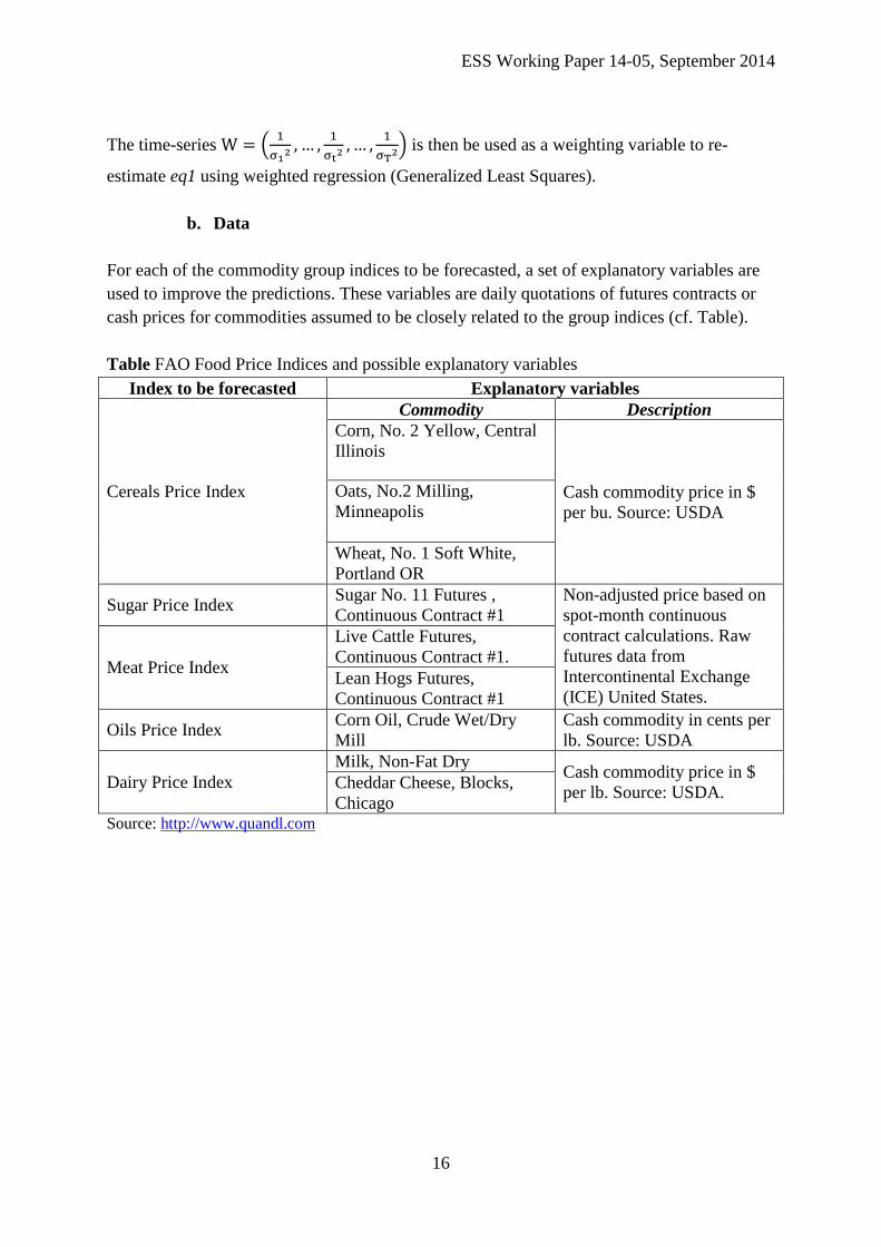
b. Data

For each of the commodity group indices to be forecasted, a set of explanatory variables are

used to improve the predictions. These variables are daily quotations of futures contracts or

cash prices for commodities assumed to be closely related to the group indices (cf. Table).

Table FAO Food Price Indices and possible explanatory variables

Index to be forecasted Explanatory variables

Cereals Price Index

Commodity Description

Corn, No. 2 Yellow, Central

Illinois

Cash commodity price in $

per bu. Source: USDA

Oats, No.2 Milling,

Minneapolis

Wheat, No. 1 Soft White,

Portland OR

Sugar Price Index Sugar No. 11 Futures ,

Continuous Contract #1

Non-adjusted price based on

spot-month continuous

contract calculations. Raw

futures data from

Intercontinental Exchange

(ICE) United States.

Meat Price Index

Live Cattle Futures,

Continuous Contract #1.

Lean Hogs Futures,

Continuous Contract #1

Oils Price Index Corn Oil, Crude Wet/Dry

Mill

Cash commodity in cents per

lb. Source: USDA

Dairy Price Index

Milk, Non-Fat Dry Cash commodity price in $

per lb. Source: USDA. Cheddar Cheese, Blocks,

Chicago Source: http://www.quandl.com

http://www.quandl.com/


17

c. Results

Figure: Observed vs. fitted values for the five commodity group indices


18

d. Forecasting

FPIs referring to the previous month are published in the first or second week of the current

month. Forecasts of the FPI for the current month are given by:

∑

Where:

- is the current month

- is determined through the first estimation of ;

- , and are determined by the weighted regression; and

- is the average of the quotations (futures contract or cash price depending on the

commodity) from the first day of the month up to the day when the forecast is made. As

regional food CPI estimates are generally disseminated during the third week of the

month, data for at least half of the current month is generally available for the forecasting.

2. Results of the Principal Component Analysis for the explanatory variables

A principal component analysis is used to reduce the number of explanatory variables for

each of the groups of variables – Food Price Indices, exchange rates, stock market indices

and oil prices. The main results of this analysis are provided for the first three groups. As

only two variables are used to measure oil prices, the first factorial axis, which contributes to

over 90% of the total variance, is selected. This analysis has been carried out using the R

package nFactors. For more information on this package and its functionalities, refer to

http://cran.r-project.org/web/packages/nFactors/nFactors.pdf.

a. FAO Food Price Indices (FPIs)

Table 1 Statistics on the principal component analysis for FPIs (selected factors highlighted)

Factors Eigenvalues

Proportion of total

variance Cumulative variance

1 1.8 0.35 0.35

2 1.2 0.24 0.59

3 0.89 0.18 0.77

4 0.69 0.14 0.91

5 0.46 0.092 1

http://cran.r-project.org/web/packages/nFactors/nFactors.pdf


19

Figure 1 Eigenvalues

b. Exchange rates against the US dollar

Table 2 Statistics on the principal component analysis for FPIs (selected factors highlighted)

Factors Eigenvalues

Proportion of total


1 4.1 0.29 0.29

2 2 0.14 0.43

3 1.3 0.095 0.53

4 1.2 0.084 0.61

5 1 0.071 0.68

… … … …

14 0.036 0.0026 1



20

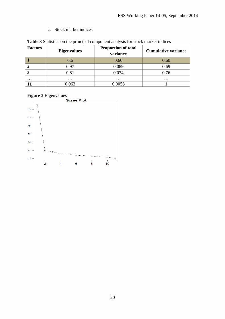
c. Stock market indices

Table 3 Statistics on the principal component analysis for stock market indices

Factors Eigenvalues

Proportion of total


1 6.6 0.60 0.60

2 0.97 0.089 0.69

3 0.81 0.074 0.76

… … … …

11 0.063 0.0058 1



21

3. Composition of macro-regions used for the Food CPIs

Northern America: United States of America, Canada, Bermuda

Central America: Costa Rica, El Salvador, Guatemala, Honduras, Mexico, Nicaragua,

Panama

South America: Argentina, Bolivia, Brazil, Chile, Colombia, Ecuador, Paraguay, Peru,

Suriname, Uruguay, Venezuela

Caribbean: Antigua and Barbuda, Aruba, Barbados, Cayman Islands, Dominican Republic,

Grenada, Haiti, Jamaica, Puerto Rico, Saint Kitts and Nevis, Saint Lucia, Saint Vincent and

the Grenadines, Trinidad and Tobago

Europe10

: all EU-27 countries, Albania, Iceland, Latvia, Norway, Switzerland, Island of

Man, Republic of Moldova, Serbia

Western Asia: Armenia, Bahrain, Cyprus, Israel, Jordan, Kuwait, Oman, Saudi Arabia,

Syrian Arab Republic, Turkey

South-Eastern Asia: Brunei, Cambodia, Indonesia, Lao, Malaysia, Myanmar, Philippines,

Singapore, Thailand

Southern Asia: Bangladesh, India, Iran, Maldives, Nepal, Pakistan, Sri Lanka

Eastern Asia: China, Hong Kong SAR, China, Macao SAR, China (mainland), Japan,

Republic of Korea

Northern Africa: Algeria, Egypt, Morocco, Tunisia

Western Africa: Benin, Burkina Faso, Côte d’Ivoire, Gambia, Ghana, Guinea, Guinea-

Bissau, Cameroon Mali, Mauritania, Niger, Nigeria, Senegal, Sierra Leone

Eastern Africa: Ethiopia, Kenya, Madagascar, Malawi, Mauritius, Mozambique, Rwanda,

Seychelles, Uganda, Tanzania, Zambia

Southern Africa: Botswana, Lesotho, Namibia, South Africa

Central Africa: Angola, Cameroon, Congo, xxGabon

10

Sub-divided into Northern, Southern, Western and Eastern Europe.


22

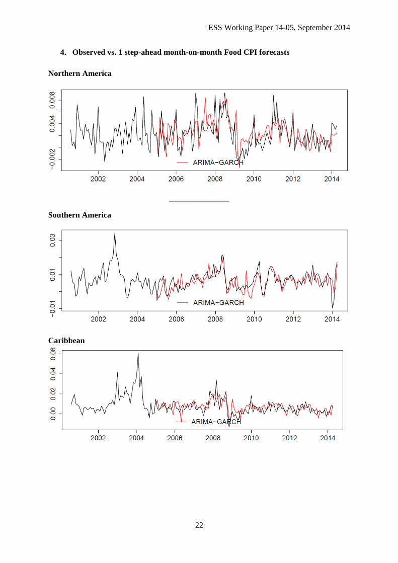
4. Observed vs. 1 step-ahead month-on-month Food CPI forecasts

Northern America

_______________

Southern America

Caribbean


23

Central America

_______________

Eastern Africa

Central Africa


24

Northern Africa

Southern Africa

Western Africa

_______________


25

Eastern Asia

South-Eastern Asia

Southern Asia


26

Western Asia

_______________

Eastern Europe

Northern Europe


27

Southern Europe

Western Europe

Contact:

Statistics Division (ESS)

The Food and Agriculture Organization of the United Nations

Viale delle Terme di Caracalla

00153 Rome, Italy

http://www.fao.org/economic/ess/ess-publications/ess-fs-papers/en/

[email protected]

I4106/1/09.14

http://www.fao.org/economic/ess/ess-publications/ess-fs-papers/en/


Date post:	27-Aug-2018
Category:	Documents
Upload:	lamhuong
View:	215 times
Download:	0 times

Nowcasting regional consumer food inflation · NOWCASTING REGIONAL CONSUMER FOOD INFLATION Franck...

Documents