NTNU Fakultet for kjemi og biologi

1

NTNU Fakultet for kjemi og biologi Norges teknisk-naturvitenskapelige Institutt for kjemisk prosessteknologi universitet

HOVUDOPPGÅVE 2000 Title: Adaptive model predictive control of chemical processes

Key words: Generalized Predictive Control, adaptive control, model development, RLS

Author: Elvira Marie Bergheim

Time period: Sept 1, 2000 – March 1, 2001

Supervisor: Prof. David E. Clough

Number of pages 128 Main report: 69 Appendix: 59

ABSTRACT One popular control strategy of model predictive control is General Predictive Control (GPC). Background and theory was studied for the GPC algorithm. The GPC algorithm was tested in both an experimental SISO case and a simulated MIMO case. The experimental case was carried out on a shell-and-tube heat exchanger while the simulated case consisted two coupled distillations columns and was carried out in HYSYS.Plant. ARX-model were used to describe the processes and they were developed from PRBS-data. The models were updated by an adapter. The adapter was based on recursive least square method. The SISO GPC showed excellent control with relatively fast rise-time, almost no overshoot and smooth actions on the control valve. The GPC controller was compared to a PID controller and the GPC had much better performance than the PID. The MIMO GPC showed poorer control and this could be caused by implementation error. The GPC was compared to a built-in MPC controller in HYSYS.Plant. The built-in MPC showed good control , much better than the MIMO GPC.

I declare that the work was carried out independent and in accordance to NTNUs regulations. Date and signature: .......................................................

2

Acknowledgement

I would like to thank prof. David E. Clough for all help with organizing my stay here inBoulder CO and supervision during the work with the thesis. In the lab Scott Whitehead andDennis Burcham have been a great help. Bradley Dunkin has been a good help with Labviewquestions.

Elvira Marie

Abstract

In recent years, model predictive control (MPC) has become more popular in industry. Onecontrol strategy of MPC is General Predictive Control (GPC). GPC computes control signalsbased on predicted outputs that are calculated from a model of the process. Background andtheory for the GPC controller was studied and then a GPC controller was implemented andused in a single-input single-output (SISO) experimental case and in a multi-input multi-output (MIMO) simulation case.

The SISO experimental case was carried out using a heat exchanger interfaced to a computer.The main goal was to control the temperature in the cold outlet stream by the hot water flowrate. An ARX-model for the process was developed from pseudo-random-binary-signal(PRBS) test. The model was updated by an adapter based on the recursive least squares(RLS) method while running tests. The control structure was cascade where the GPCcontroller was the master controller that measured the temperature and calculated a set pointfor the slave controller. The slave controller controls directly the hot water flow rate.

The GPC controller was tested with several different cost and control horizons, weightingparameters and forgetting factors. The most important parameter to the performance was costhorizon. If the cost horizon was too long, the prediction of the output became poor becauseof uncertainty in the system. If the cost horizon is too short, the prediction did not include thedynamics of the process. A longer control horizon gave more active control but it mightcause more fluctuations in the manipulated variable compared to a shorter control horizon.The weighting of the control signal needed to be quite conservative or else it producedoscillations in the process. If the weighting value was too conservative, the rise-time to thesystem became longer than necessary. The forgetting factor had no influence on the controlperformance and the control horizon had minor influence on the performance.

The GPC controller was then compared with a PID controller for the same process in acascade. The PID controller was not as effective in smoothing out oscillations as the GPCcontroller. In a step test, the rise-time was shorter for the PID controller. However, the setpoint to the slave controller changed between fully open and fully closed valve which makesthe output oscillate and caused unnecessary wear and tear on the valve. The control signalchanges smoothly when using the GPC controller, and there were minimal oscillations.

The MIMO simulation case was arranged in HYSYS.Plant. The process included twodistillation columns coupled through recycle streams, which separated natural gas liquid(NGL) into ethane and propane and a bottom stream that went on to further separation. Thesimulated process has local PID controllers and a multivariable GPC controller connected tothe second column.

An ARX-model based on data from PRBS-tests is used in GPC. The GPC included also anadaptive part, which updated the model. The adapter is based on the RLS method. Tests werecarried out by decreasing the ethane molar flow rate in the feed stream. Performance of the

4

GPC controller was evaluated for several different cost horizons, control horizons andcontrol signal weighting matrices. The performance is particularly sensitive to cost horizonand control signal weighting.

The GPC controller was compared with the MPC controller that is built into HYSYS.Plant.The built-in MPC used a first order plus dead time (FOPDT) model to predict outputs. Thecontroller was tested on the exactly same process with the same changes in ethane molar flowrate in the feed stream. Built-in MPC showed smooth control for several parameters.

The built-in MPC was preferred to the GPC because it showed good performance and wasvery simple to use. The built-in MPC was not as sensitive to parameter choices as the GPCcontroller. However, the GPC controller would probably be better if the process had morecomplex dynamics, which would be poorly approximated by FOPDT.

In both the SISO experimental case and the MIMO simulation case the cost horizon andcontrol signal weight was found to be important to the performance of the GPC controller.The control horizon was of lesser importance, and the forgetting factor in the RLS made nodifference in the GPC performance.

5

Contents

1. Introduction 8

2. Theory Experimental Case 9

2.1 Pseudo-random-binary-signal tests................................................................................. 92.2 Model development ........................................................................................................ 92.3 The General Predictive Controller ................................................................................ 10

2.3.1 Recursion of the Diophantine equation .................................................. 112.3.2 The Predictive Control Law ................................................................... 122.3.3 Cost function with constrains on control signal ..................................... 14

2.4 Cascade control ............................................................................................................. 152.5 The Recursive Least Squares method........................................................................... 162.6 PID Controller in discrete time ..................................................................................... 20

3. Experimental Phase - Singlevariable 21

3.1 Process description of heat exchanger and additional equipment ................................ 213.2 Calibration..................................................................................................................... 233.3 Model development ...................................................................................................... 243.4 Implementation of the GPC Controller......................................................................... 253.5 Implementation of the adaptive controller.................................................................... 273.6 Implementation of the PID controller ........................................................................... 283.7 Testing the controllers.................................................................................................. 28

4. Results From Experimental Phase 29

4.1 Results using GPC controller........................................................................................ 294.2 Compare GPC and PID controller ................................................................................ 31

5. Discussion Experimental Phase 33

5.1 Equipment ..................................................................................................................... 335.2 Implementation ............................................................................................................. 335.3 Observations ................................................................................................................. 35

6. Theory multivariable case 38

Contents

6.1 ARX-model in multivariable case ................................................................................ 386.2 Diophantine equation in multivariable case.................................................................. 386.3 GPC in multivariable case ............................................................................................ 406.4 Including constraints in the GPC algorithm.................................................................. 416.5 Recursive least squares parameters estimation in multivariable case........................... 43

7. Experimental Simulation Phase 45

7.1 Description of simulation process................................................................................. 457.2 Control structure ........................................................................................................... 497.3 Implementation ............................................................................................................. 51

7.3.1 Implementation of the GPC controller ................................................... 517.3.2 Implementation of the built-in MPC ...................................................... 53

8. Simulation Results 55

8.1 Results using GPC including RLS adapter ................................................................... 558.2 Results using built-in MPC in HYSYS.Plant ............................................................... 57

9. Discussion Multivariable Case 58

9.1 The separation process.................................................................................................. 589.2 The GPC controller ....................................................................................................... 609.3 The built-in MPC Controller......................................................................................... 629.4 Comparison of the GPC Controller and the built-in MPC Controller .......................... 639.5 Comparison using GPC in experimental phase and simulation phase.......................... 63

10.Conclusion 66

References 68

Glossary 69

Appendix 71

Introduction

8

1. INTRODUCTION

Model predictive control (MPC) was introduced in the late seventies and has developedsignificant since then. The term MPC does not entitle a specific control strategy but includinga range of control methods. Commons for the control methods are that a process model isused to predict output in future time to obtain control signals by minimizing an objectivefunction. The different control methods only differ in the model used to represent the processand the noises and the cost function to be minimized.

One of the MPC control strategies is the Generalized Predictive Control (GPC) and wasdeveloped by Clarke, Mohtadi and Tuffs. Their main work on the method was presented in1987. The method has been implemented in many industrial applications, showing goodperformance and a certain degree of robustness for a wide range of plants.

This thesis has studied GPC in both a SISO experimental case and a MIMO simulation case.They were treated separately in this thesis. The experimental part included most of the theorythe thesis was based on, but the simulation part treats supplemental parts of the theory whenextending the algorithm from a single variable case to a multivariable case.

The thesis was carried out at University of Colorado at Boulder in fall 2000 and spring 2001.

Theory Experimental Case

2. THEORY EXPERIMENTAL CASE

2.1 Pseudo-random-binary-signal tests

To develop a model for a process, pseudo-random-binary-signal (PRBS) can be used fordeveloping data. The PRBS binary inputs, either u1 or u2, are selected randomly in chosentime interval ∆t. The responses are observed and recorded. A typical PRBS input sequencecan be as depicted in figure 2.1, from [9].

Figure 2.1 Illustration of a typical PRBS input

It is important to avoid missing dynamics information from the system, so the samplinginterval has to be chosen properly. The sampling interval has to be long enough so the systemhas a chance to show responses, and not too short so missing dynamics is avoided. To detectdeadtime and responstime, a steptest can be executed. The difference between the binary input signals needs to be big enough to produce asignificant difference in the output. The binary inputs should also be selected in the operatingrange and the inputs should not reach saturation.

2.2 Model development

All MPC methods need a model for the process to predict the output. It is important that themodel gives a good description of the process to avoid poor prediction. An autoregressivemodel with input, also named ARX can be used. This model can be identified from PRBS-test data as described by Clough [6]. An ARX-model is on the form

t

u2

u1

4∆ 8∆ 12∆

9


(2.1)

where A and B are the model parameters and they are functions of the backward shift operatorq-1. y(t) is the output, u(t) is the input, d is the delay in the model and e(t) is the noise. The Aand B have the form:

(2.2)

(2.3)

where na and nb are the order of A and B respectively.

Aikake’s Final Prediction Error (FPE) can be used as indicator to select the best modelbetween the different model structures. FPE penalizes over-parameterization of the modeland prefer less complex models. Fitting PRBS-data to an ARX-model can be done by forinstance Matlab with the function arx.

2.3 The General Predictive Controller

One popular predictive control algorithm is the Generalized Predictive Control (GPC). TheGPC method was proposed by Clarke et al. [3]. The basic idea of GPC is to calculate asequence of future control signals in such way that it minimize a multistage cost functiondefined over a prediction horizon.

The theoretical deduce of the GPC controller is derive from Camacho and Bordons [1] andClarke et. al. [3]. Most single-output single-input (SISO) plants can be described by aControlled AutoRegressive and Integrated Moving Average (CARIMA) model whenconsidering operation around a particular set-point and after linearization. The CARIMAmodel is given by

(2.4)

with ∆=1-q-1 and C(q-1) is the noise polynomial and has the same form as A(q-1) given inequation (2.2), and q-1 is the backward shift operator. y(t) is the output, u(t) is the input, d isthe dead-time and e(t) displays the noise. The noise is assumed as zero mean white noise. Forsimplicity, the C polynomial is chosen to be 1. To derive a j-step predictor of y(t+j), consider the Diophantine equation

(2.5)

where Ej and Fj are polynomials uniquely defined given A(q-1) and the prediction interval j.The degrees of Ej and Fj polynomials is j - 1 and na respectively.

A q 1–( )y t( ) B q 1–( )u t d–( ) e t( )+=

A q 1–( ) 1 a1 q 1– a2 q 2– … an a q n a–+ + + +=

B q 1–( ) b0 b1 q 1– b2 q 2– … bn b q n b–+ + + +=

A q 1–( )y t( ) q d– B q 1–( )u t 1–( ) C q 1–( ) e t( )∆

---------- +=

1 Ej q 1–( )A q 1–( )∆ q j– Fj q 1–( )+=

10


If equation (2.4) is multiplied with Ej ∆qj we get

(2.6)

Considering Diophantine equation in (2.5), equation (2.6) can be written as

(2.7)

which can be rewritten as

(2.8)

As the degree of polynomial Ej(q-1) is j-1 the noise terms in equation (2.8) are all in thefuture. The optimal prediction of y(t+j) is therefore,

(2.9)

where Gj(q-1) = EjB.

In GPC a whole set of predictions is considered, for which j runs from a minimum up to alarge value, termed as the minimum and maximum prediction horizons. A system with a deadtime d will the prediction process for j< d only depends on the available data,but for assumptions need to be made about future control actions.

2.3.1 Recursion of the Diophantine equation

To solve the prediction in equation (2.9), the polynomials Ej and Fj are needed in addition tothe model parameters A and B. The polynomials Ej and Fj can be obtained recursively fromthe Diophantine equation, given in equation (2.5).

Suppose for clarity of notation E = Ej, R = Ej+1, F = Fj, S = Fj+1 and defined as A∆ . TheDiophantine equation in (2.10) corresponds to the prediction for and equation(2.11) corresponds to the prediction for .

(2.10)

(2.11)

Subtracting equation (2.10) from equation (2.11) gives

(2.12)

The polynomial R - E is of degree j and may be split into to parts

Ej q 1–( )A∆y t j+( ) Ej q 1–( )B q 1–( )∆u t j d– 1–+( ) Ej q 1–( )e t j+( )+=

1 q j– Fj q 1–( )–( )y t j+( ) Ej q 1–( )B q 1–( )∆u t j d– 1–+( ) Ej q 1–( )e t j+( )+=

y t d+( ) Fj q 1–( )y t( ) Ej q 1–( )B q 1–( )∆u t j d– 1–+( ) Ej q 1–( )e t j+( )+ +=

y t j t+( ) Gj q 1–( )∆u t j d– 1–+( ) Fj q 1–( )y t( )+=

y t j t+( )j d≥

Ay t j t+( )

y t j 1 t–+( )

1 EA q j– F+=

1 RA q j 1+( )– S+=

0 A R E–( ) q j– q 1– S F–( )+=

11


(2.13)

where is a polynomial of degree smaller and equal to j-1 and rj is a scalar. The equation (2.12) then becomes

(2.14)

Since is monic, that is all coefficients are unequal to zero and first coefficient equals 1, needs to be equal to zero. This indicates that . As as ha unit leadingelement, we have

(2.15)

(2.16)

for i = 0 to the degree of S(q-1) and

(2.17)

(2.18)

Given the plant polynomials A(q-1) and B(q-1) and one solution of Ej(q-1) and Fj(q-1), thenequation (2.15) and equation (2.16) can be used to obtain Fj+1(q-1). Vector Ej+1(q-1) can beobtained by equation (2.17).

To initialize the iterations, the Diophantine equation can easily be solved for j = 1, that is. Since the leading element of is 1, then is E1 = 1 and F1 = q(1- ).

2.3.2 The Predictive Control Law

The GPC algorithm consists of applying a control sequence that minimizes a multistage costfunction of the form

(2.19)

where is an optimum j-step ahead prediction of the system output on data up totime t, N1 and N2 are the minimum and maximum costing horizons, Nu is the control horizon,δ(j) and λ(j) are weighting sequences and w(t + j) is the future reference trajectory. The costhorizon N can be expressed as

. (2.20)

R E– R rj qj–+=

R

A R q j– q 1– S F– A r j+( )+ 0=

A RS q F Arj–( )= A

r j f0=

si f i 1+ a i 1+ rj–=

R q 1–( ) E q 1–( ) q j– rj+=

Gj 1+ B q 1–( )R q 1–( )=

1 E1 A q 1– F1+= A A

J N1 N2 Nu, ,( ) δ j( ) y t j t+( ) w t j+( )–[ ] 2 λ j( ) ∆u t j 1–+( )[ ] 2

j 1=

Nu

∑+

j N1=

N2

∑=

y t j t+( )

N N2 N1– 1+=

12


and represents how far into the future the predictions are made when calculation thecontroller output. The control horizon NU represents the number of controller moves into thefuture that will be made to achieve the final set point.

The set of j ahead optimal predictions is given by equation (2.9) and can be expressed as

(2.21)

which can be written in matrix form as

(2.22)

where

The last two terms in equation (2.22) depend only on the past outputs and past inputs andcorresponds to the free response, f, leading to

(2.23)

where the vectors y, u and f have dimension N x 1.

y t d 1 t+ +( ) Gd 1+ ∆u t( ) Fd 1+ y t( )y t d 2 t+ +( )

+Gd 2+ ∆u t 1+( ) Fd 2+ y t( )

…y t d N t+ +( )

+

Gd N+ ∆u t N 1–+( ) Fd N+ y t( )+

==

=

y Gu F q 1–( )y t( ) G' q 1–( )∆u t 1–( )+ +=

y

y t d 1 t+ +( )y t d 2 t+ +( )

…y t d N t+ +( )

= u

∆u t( )∆u t 1+( )

…∆u t N 1–+( )

=

G

g0 0 … 0g1 g0 … 0… … … …

gN 1– gN 2– … g0

= F q 1–( )

Fd 1+ q 1–( )

Fd 2+ q 1–( )…

Fd N+ q 1–( )

=

G' q 1–( )

Gd 1+ q 1–( ) g0–( )qGd 2+ q 1–( ) g0– g1 q 1––( )q2

…Gd N+ q 1–( ) g0– g1 q 1–– …– gN 1– q N 1–( )––( )qN

=

y Gu f+=

13


If equation (2.23) is inserted in the cost function in equation (2.19), the cost function can bewritten as

(2.24)

where , λ(j) is assumed

constant and δ(j) is assumed as one. Multiplying out equation (2.24) gives:

(2.25)

where

(2.26)

By making the gradient of J with respect to u equal to zero, the minimum of J can be found,assuming there are no constraints on the control signal. This gives

(2.27)

It is only the first element of vector u that is actually sent to the process, so the control lawis given by

(2.28)

where is the first row of . This control law can be implemented inMatlab.

2.3.3 Cost function with constrains on control signal

If there are constraints on the control signals, the control law given in equation (2.28) needsto be written as a function of u instead of ∆u. The process output can be written as in equation. The vector of future control increments is given by

(2.29)

which can be written as

J Gu f w–+( )T Gu f w–+( ) λ uT u+=

w w t d 1+ +( ) w t d 2+ +( ) … w t d N+ +( )T

=

J 12--- uT Hu bT u f0+ +=

H 2 GT G λ I+( )bT 2 f w–( )T Gf0 f w–( )T f w–( )

===

u H 1– b– GT G λ I+( ) 1– GT w f–( )= =

u t( ) u t 1–( ) gT w f–( )+=

gT GT G λ I+( ) 1– GT

u k( ) u k 1–( )–u k 1+( ) u k( )–

…u k N+( ) u k N 1–+( )–

1 0 0 … 01– 1 0 … 0

0 1– 1 … 0… … … … …0 0 0 … 1

u k( )u k 1–( )

…u k N+( )

u k 1–( )0…0

–=

14


(2.30)

The equations for the future control signal is substituted in the equation of future predictions,equation , and we get

(2.31)

where G’ is a lower triangular matrix and f2 can be expressed as

(2.32)

The cost function can now be expressed as a function of the future control actions U,

(2.33)

Written J(U) in a quadratic form,

(2.34)

where

(2.35)

The cost function is now a function of future control actions and constrains can easily beadded on the control signals. The control signal can be found by minimizing the cost functionin equation (2.34) with the constrains added to the minimizing problem. The minimizingproblem can be solved in for instance Matlab with the function fmincon or solved as a QP-problem with function quadprog.

2.4 Cascade control

Cascade control can be useful when disturbances are associated with the manipulatedvariable or the final control element exhibit nonlinear behavior. Nonlinear behavior can forinstance be significant hysteresis in a valve. The output signal of the master controller servesas the set point for the slave controller. The secondary loop is a faster loop that is locatedinside the primary control loop.

Dependent on the control problem, the slave controller can be a PI controller in velocity

u DU f1–=

y G DU f1–( ) f+ G'U f2+= =

f2( ) i f( ) i gi u k 1–( )+=

J U( ) G'U f2 w–+( )T G'U f2 w–+( ) λ DU f1–( )T DU f1–( )+

UT G'TG' λDTD+( )U 2 f2 w–( )TG' λ f1D–[ ] U f2 w–( )T f2 w–( ) λ f1Tf1+ + +

=

=

J U( ) 12--- UT H'U b'U f'+ +=

H' 2 G'T G' λ DT D+( )b' 2 f2 w–( )T G' λ f1 D–[ ]f' f2 w–( )T f2 w–( ) λ f1

T f1+

===

15


mode. The theoretical deduce of PI controller in velocity mode is derived from Seborg et al.[12]. The velocity form of the PI controller does not compute summations which is neededin position mode and therefore windup is avoided. The velocity mode does not requirespecification of the bias term.

The design equation for a PI controller in velocity mode can be found from the generalposition mode for a PI controller, given in equation (2.36),

(2.36)

where u is the control signal, Kc is the gain, e represent the error between the measurementand the set point, τI is the integral time and b is the bias. The velocity mode is found by taking the time derivative of equation (2.36).

(2.37)

With approximations for the derivative, this becomes

(2.38)

In the discrete case this can be expressed as

(2.39)

Equation (2.39) can be implemented directly in virtual instrument, for instance Labview.

2.5 The Recursive Least Squares method

The deduce of the recursive least square method is based on a handout from Clough [5]. Anadapter tasks is to adjust the controller parameters automatically to compensate for changingprocess condition. This can be very useful when the process conditions changes in time. Aillustration of single-input single-output process is displayed in figure 2.2.

Figure 2.2 Illustration of a single-input single-output process.

The adaptive controller use recursive least squares (RLS) method to calculate the A and B

u t( ) Kc e t( ) 1τ I---- e t'( ) t'd

0

t

∫+

b+±=

du t( )d t

-------------- Kcde t( )

d t-------------- e

τ I----+

±=

∆u∆ t------- Kc

∆e∆ t------- e

τ I----+

±=

ui un 1– Kc 1 ∆ tτ I------+ en en 1––

±=

ProcessInput Output

y(k)u(k)

16


polynomial in the model. The A and the B polynomial is as given in equation (2.2) andequation (2.3). The degree of the A polynomial is na and the degree of the B polynomial isnb. Define the parameter column vector as

(2.40)

The output vector is defined as

(2.41)

where N is the cost horizon and d is the dead-time. The matrixϕ is defined as

(2.42)

The error vector is defined as

(2.43)

The evaluation of the model for the data set can be represented by

(2.44)

The loss function can be written as the sum of the squares of the residuals

(2.45)

To minimize the loss function can be done by setting

for i = 1 to na + nb (2.46)

The result from minimizing the loss function is

(2.47)

The derivation of the minimization is given in [5]. The RLS algorithm can be described as infigure 2.3. The same algorithm can be used in Matlab implementation.

β a1 …… an a b0 … bn b

T=

yy 1 na d+ +( )

…y N na d+ +( )

=

ϕy na d+( )– … y 1 d+( )– u nb( ) … u 1( )

… … … … … …y na d N 1–+ +( )– … y N d+( )– u nb N 1–+( ) … u N( )

=

ee 1 na d+ +( )

…e N na d+ +( )

=

e y ϕβ–=

V eT e=

∂V∂β i-------- 0=

β ϕ T ϕ[ ] 1– ϕ T y=

17


Figure 2.3 The RLS Parameter Estimation Algorithm

ψ N 1+( )

Obtain measurement y(N+1)

Update vector of past data Obtain past

output

u(N-d)

y N 1+( ) ψT N 1+( ) β N( )=

K N( ) P N( )ψ N 1+( )γα ψT N 1+( )P N( )ψ N 1 ]+( )+[ ]

-------------------------------------------------------------------------------------------------=

β N 1+( ) β N( ) K N( ) y N 1+( ) y N 1+( )–[ ]+=

Do I haveenough data?

YES NO

Compute model prediction

Update gain vector

Update parameter estimates

P N 1+( ) 1γ--- I K N( )–[ ]ψ T N 1+( ) ] P N( )=

Compute covariance matrix for next iteration

18


In figure 2.3 ψ is a vector that contains the past values of measurement and control signalswith the size (m+n) x 1 and has the form

(2.48)

The scalar is the prediction of the measurement based on the model. K is the gain vectorand γ is the forgetting factor. The forgetting factor weight out or "forget" gradually the pastvalues. The forgetting factor has a value between 0 and 1, and the closer γ is to 1, the slowerthe algorithm "forgets" the past values. In other words, it becomes more conservative. β is aparameter vector as described in equation (2.40). P is the covariance matrix and is defined by

(2.49)

where

(2.50)

The parameter α indicates the error the model has not manage to include compare to theprocess. A value of α can be found in the result from fitting ARX-model based on PRBS-data. Matrix I is the identity matrix which has the same dimension as K. The question "Do Ihave enough data?" is a question if ψ is filled up with data from the process or not.

To initialize the algorithm, values for , P and α is needed. The initialization can done bysetting

(2.51)

where c is a large number. The vector can also be initialized by using the A and Bparameters in the ARX-model.

To update the model parameters, RLS needs changing inputs to the algorithm. This is usuallynot a problem in real world but with small, separated systems with no turbulent flow orsimulations with no disturbances, this needs to be considered. With too little noise in thesystem the matrixes in the RLS can become singular and weird values for the A and the Bparameters can occur which again gives poorly prediction of the outputs.

ψ N 1+( )

y N( )–…

y N na– 1+( )–u N d–( )

…u N d– nb– 1+( )

=

y

P N( ) ϕ T N( )ϕ N( )[ ] 1– α=

α v ar e k( ){ }=

β

β 0( ) 0P 0( ) cI

==

β

19


2.6 PID Controller in discrete time

The theoretical deduce of PID digital controller is derive from Seborg et al. [12]. Design equation for digital PID controller is based on the ideal, continuous (analog) PIDcontroller, which is described as

(2.52)

where u(t) is the control signal, Kc is the gain, e(t) represent the error between themeasurement and the set point, τI is the integral time, τD is the derivative time and b is thebias. To convert this expression to its digital equivalent, the following finite differenceapproximations are used

(2.53)

When the approximations in equation (2.53) are introduced in the ideal analog PID, theposition form of the digital PID controller can be written as

(2.54)

The position form of the PID controller can now be implemented as the control low becauseit yields the valve of the controller output directly. The controller can be implemented in forinstance Labview.

u t( ) K± c e t( ) 1τ I---- e t'( ) t' τ D

de t( )d t

--------------+d0

t

∫+ b+=

e t'( ) t' ek ∆ tk 1=

n

∑≈d

ded t------ en en 1––

∆ t-------------------------≈

0

t

∫

u t( ) K± c en∆ tτ I------ ek

τ D

∆ t------ en en 1––( )+

k 1=

n

∑+=

20

Experimental Phase - Singlevariable

3. EXPERIMENTAL PHASE - SINGLEVARIABLE

The experimental part of this paper tested the general predictive control (GPC) algorithmwith a recursively least square (RLS) adapter on a single-input single-output (SISO) process.

3.1 Process description of heat exchanger and additional equipment

The heat exchanger was an already existing unit interfaced to a converter and a computer inthe Chemical Engineering Laboratory at University of Colorado. The heat exchanger isillustrated in figure 3.1.

The heat exchanger was a shell-and tube type. The cold water flowed inside the tubes and thehot water flowed outside the tubes. It had four termocouples that were placed at each inletsand outlets. The heat exchanger had also a valve on each inlet stream that was controlled byair pressure. The valve on the hot water inlet had also a valve positioner. In addition therewere safety valves on each stream.

The computer used Labview software from National Instruments Corp., a graphicalprogramming language to create block diagram structures. Program modules in Labview arecalled virtual instruments (VI’s).

The heat exchanger was connected to a computer by analog-to-digital converter and digital-to-analog converter. The interface between the heat exchanger and the computer is presentin figure 3.2.

The termocouples gave signals in mV and needed to be converted to oC. The voltage signalswere sent to the computer and displayed in Labview’s virtual instrument (VI).

The flow was measured in differential pressure (∆P). The differential pressure was convertedto current in the pressure-to-current (P/I) converter. This signal was again converted tovoltage in the current-to-voltage (I/V) converter before it reached the computer. The flowsignals from the computer followed the opposite direction and were converted to pressure,which made the valves move. This is displayed in figure 3.3 including the range at eachconversion.

21


Figure 3.1 Diagram of the heat exchanger

I/P

Vc

DPT

qc

Cold water inlet

Tci

I/P

DPT

Thi

Vc

qh

Hot waterinlet

Tco

Cold water drain

Hot water drain

Tco

22


.

Figure 3.2 Diagram of the interface between the computer and the heat exchanger

.

Figure 3.3 Signal processing between the computer and the hot water valve at the heat exchanger

3.2 Calibration

The temperature- and flow measurements needed to be calibrated before running tests. First the process was implemented in Labview and the signals were connected to the rightchannel in the D-to-A converter. The Labview diagram was based on an existing program

Inputs

MultiplexerI/V

I/V

Thi

Tho

Tci

Tco

converter

converter

A-to-Dconverter

V/I

V/I

Outputs

Vh

Vc

qh

Computer

D-to-A

D-to-A

I/P

I/P

qc P/I

P/I

Output fromD-to-A converter

5 V

0 V

V/I

4 mA

20 mA

I/P

15 psi

3 psi

Valve positioner

Hot watervalve

Open

Closed

23


that is used in a lab course at University of Colorado. Prof. D.E. Clough at University ofColorado made this program. The Labview diagram is displayed in appendix A.

The flow rate was measured by collecting the flow in a bucket over a certain time interval,while the voltage displayed in Labview’s VI was noted. The collected water were weighted,and with the assumption that 1 kg equals 1 liter; the flow rate was expressed in l/min. Thiswere done to both the hot water and the cold water flow.

When the flow was measured, the current was measured in the current-to-voltage (I-to-V)converter with a multimeter. The zero and the span in the I-to-V converter were adjusted tozero flow and difference between zero and maximum flow respectively. This were done bothwith the hot water and the cold water flow.

The flow measurements were plotted against the voltage in an Excel worksheet and therelation between the flow and the voltage were found. The theory background for flow andvoltage relation is displayed in appendix B. When the voltage dropped below a certainthreshold value it became necessary to set the flow equal to zero to avoid numericalproblems, due to the square root in the relation between flow and voltage. Zero flow wasobserved for the hot water when the voltage drops below the threshold value. The cold waterflow was about 2 l/min when the voltage dropped below the threshold value. The cold watervalve never managed to close the valve totally. The relation between flow rate and volt wasimplemented in Labview.

During the calibration tests, hysteresis was discovered on both the hot water valve and thecold water valve. The hysteresis was less on the hot water valve than the cold water valve.This was expected due to the valve positioner placed on the hot water valve. The relationshipbetween the flow and the square root of the voltage became poorly at high voltage, so thisarea was avoided in the further tests.

For the termocouples there existed already a relation between temperature in oC and voltagein mV from earlier experiments on the heat exchanger. The termocouples were checkedagainst standard thermometers in ice and boiling water respectively. The temperatures fromthe termocouples were plotted against the temperatures from the standard thermometers andrelations were found. The relation between mV and oC was implemented in Labview.

3.3 Model development

The GPC algorithm needed a mathematical model that describes the process, as explained inchapter 2.3. PRBS-tests was chosen to generate process data and used to develop an ARX-model.

A VI in Labview was made to generate the PRBS-tests, based on the Labview program madefor calibration. The diagram of the VI is displayed in appendix C. PRBS-test was carried out

24


with binary inputs from four different ranges. Both low and high values for both hot and coldwater were used as binary input. The binary input-values for the hot water valve settings werefound by try and fail. Input to PRBS was a gauge-value from Labview’s VI and was in therange 0 to 5. To find a suitable sampling interval, a step test was executed to find the deadtime to the system. The dead time was 3-6 seconds, depending on the flow rate. The samplinginterval in the PRBS-test was chosen to be 3 seconds. Each PRBS-tests ran for about 10minutes. The test data was recorded in a text file and used for model development. Four models were developed, one for each range the PRBS-test were done. ARX-modelswere developed by Matlab using data from the PRBS-tests. The Matlab algorithm used fordeveloping models is displayed in appendix F.1. An example for how the PRBS-test wherecarried out, is shown in appendix D.

3.4 Implementation of the GPC Controller

A VI in Labview was implemented to serve GPC. The VI was based on the VI from PRBS-tests, and the diagram is displayed in appendix E.

The implementation of the GPC controller could be divided into two parts. The Labview partgot the signals from the heat exchanger in a certain time interval and sent signals to the hotwater valve to control the cold water outlet temperature. The Matlab part receivedinformation about the past outputs and inputs from Labview. Based on the information fromLabview, the GPC algorithm calculated the future control actions. The first control actionwas received in Labview, which sent the signal to the hot water valve.

First, the control law given in equation (2.28) was implemented in Matlab. In the control lawthe control signal was not limited in the algorithm. The control signal became limited whenit was sent to the heat exchanger. Test with the GPC without limited control signal showedpoorly control. The control gave offset and oscillations with periods about 30 seconds. Thismay be caused from the unlimited control signal sent to the process.

Therefore a new cost function with constrains, as presented in chapter 2.3.3, wasimplemented in Matlab. The GPC algorithm implemented in Matlab is presented in appendixF.2, with additional functions in appendix F.3 and appendix F.4.

Tests showed oscillations in the system even though the control signals were limited. Theoscillations had two periods, one faster with periods about 12 seconds and the other slowerwith periods about 120 seconds. The amplitudes were approximately 0.7oC and 2oCrespectively. This pattern did not occur when the GPC with constraints was connected to themodel instead of the process. When the GPC "controlled" the model, the control was perfect.From that observation, the equipment was the cause to the oscillations. The oscillationsoccurred probably because of the hysteresis in the hot water valve.

25


To reduce hysteresis, a cascade was implemented with a flow controller as slave and the GPCas the master controller. The cascade was set up as illustrated in figure 3.4.

Figure 3.4 Illustration of the heat exchanger with cascade control

For the slave controller, a PI controller in velocity mode was used as described in chapter2.4. The slave controller was implemented in Labview, by using equation (2.39). Step testsin different operating areas were performed in manual mode to find values for the parametersKc and τI. The tuning parameters were found by Skogestad’s tuningsrules [13]. Mean valuesof the tuning parameters are found by average the different parameters from the different steptests. The sampling time to the slave controller was set to 0.25 seconds. With a gain Kc = 0.06and τI = 1.0, the slave controller worked properly.

When the slave controller was implemented in Labview, the process from the GPC point ofview changed. GPC algorithm gave now a set point to the slave controller instead of a gauge-value to the hot water valve. In other words, the process now contained a slave controller,and a new PRBS-test was performed to obtain a new model for the GPC. Only one PRBS-test was performed in the middle flow area, because the model developed from the PRBS-test supposed later to be updated by an adapter. More detailed description of the PRBS-testis present in appendix D.

One problem with the Labview program implemented for the cascade control was the timing.The GPC controller and the slave controller did not operate independent in time. So when

DPT

Hot waterinlet

Hot wateroutlet

Cold water inlet

Cold wateroutlet

TT

GPC

FCFT

26


the Labview program ran, it let the GPC algorithm work first and find the optimal controlsignal. This signal was sent as a set point to the slave controller. After GPC finished itscalculations, then the slave controller started to correct the valve opening due to set point. Sothe slave controller actually waited for the GPC controller to finish its job.

3.5 Implementation of the adaptive controller

The adaptive controller job was to update the model, which the GPC controller used forprediction. The model might be changed with different flows and temperatures. The adaptivepart was based on recursive least squares and implemented as a function in Matlab. TheMatlab algorithm is shown in appendix F.4.

To check that the adapter worked properly, the adapter was tested before connected to theGPC. Tests were done by sending PRBS-signals with different average set points to theadapter. The model parameters were observed and model changes could be detected.

When the adapter was connected to GPC, it received the values for the predicted inputs andthe past outputs through the GPC algorithm. The adapter was actually not directly linked toLabview but only to the GPC algorithm. With recursive least squares method, the adaptercalculate the coefficients to the A and B polynomial in the model and gave the new valuesfor A and B back to the GPC. The data flow is displayed in figure .

Figure 3.5 The interface between the process, GPC and RLS including the data flow

Process includedslave controller

GPC

Hot waterflow Temp. cold

water outlet

RLS

AB

Costhorizon

Set-point

Controlhorizon

27


3.6 Implementation of the PID controller

The GPC controller was replaced with a PID controller for comparison. A PID controller inposition mode was chosen. The Labview program for the PID controller was based on anexisting program from Prof. D.E. Clough at University of Colorado at Boulder. The Labviewdiagram is displayed in appendix H.

A step test was carried out to collect data from the process. The sampling time were set to1.5 second, which was the fastest sampling time possible due to the CPU time. The step testdata were treated in control software called Control Station to obtain values for the processgain (Kc), integral time (τI) and derivative time (τD). The parameters were tested andadjusted. Skogestad’s tuning rules [13] was also applied on the same step test data to developtuning parameters for the PID controller. The tuning parameters developed by ControlStation and the parameters developed with Skogestad’s tuning rules were very similar. Thiswas expected when both methods are based on Internal Model Control (IMC).

Since the sampling time was shorter when using the PID controller compare when using theGPC, the conditions for the slave controller changes. The slave controller was implementedin the same way as when the GPC was the master controller. Because of the implementationwhere the master controller and slave controller were in the same loop, the number of timesthe for-loop for the slave controller was executed was decided of computation time of mastercontroller and sampling time. The sampling time was shorter for the PID controller, but thecomputation time was significantly shorter compared to the GPC controller. The number oftimes the for-loop for the slave controller was executed was increased from 5 to 11.

3.7 Testing the controllers

When testing both GPC controller and PID controller, the test were all tried to be as equal aspossible. The same changes in set point and disturbances were therefore done in all tests.First, during start up, the set point for the cold water outlet temperature was set to 28 oC.When the output settled down as much as it seemed possible, the set point was increased to33 oC. After the output settled down after the set point change, the set point was decreasedto 27 oC. During this set point changes the cold water flow was around 5 l/min. While the setpoint was 27 oC, the cold water flow, considered as a disturbance, was increased to 15 l/min.Then the cold water flow was decreased to 6 l/min before the test finished.

28

Results From Experimental Phase

4. RESULTS FROM EXPERIMENTAL PHASE

4.1 Results using GPC controller

To test the GPC controller several tests were carried out with changing parameters in theGPC algorithm. In the GPC algorithm the parameters cost horizon (N), control horizon (NU)and the control-weighting λ needed to be decided. In addition the forgetting factor in theadapter needed to be set. The sampling interval was 4 seconds, because this was the fastesttime the computer could work through the virtual instrument and the functions in Matlab.

The parameters in the GPC algorithm were initially chosen based on suggestions from Clarkeet al. [3] and Clarke et al. [5] and then other parameters where tried out, based on theperformance in the earlier test that where carried out.

The minimum costing horizon value was based on that N1 could be chosen as the dead timein the process or more to minimize computations, from Clarke et al. [3]. Since the dead timewas observed to be longer than one sampling interval at lower flows, N1 was chosen to be 2in all tests.

The maximum costing horizon value should be chosen so it encompassed the response,which was significantly affected by the current control. N2 should be at least greater than thedegree of B(q-1), or more typically N2 is set to approximate the rise-time of the plant, fromClarke et al. [3]. The degree of the B polynomial was seven, from the ARX-modeldeveloped. The rise time for the process was about 30 seconds, which is about 8 samples witha sampling interval of 4 seconds. Several values for N2 was tested among therecommendations.

The control horizon NU equals one is generally satisfactory for a process plant, while a"difficult" plant requires that the control horizon is about the same as number of unstable orunderdamped poles, from Clarke et al. [5]. Several cost horizons values were tested from therecommendations.

The control weighting factor, λ, can be selected as zero or λ can be selected as a smallnumber because it helps numerical robustness, from Clarke et al. [5]. The weighting factorwas changed between four different values to detect how it affected the performance of thecontroller. The forgetting factor in the RLS adapter was changed between two values.Typical choices of forgetting factor are in the range between 0.98 and 0.995, from Ljung etal. [9].

Several tests were executed and the parameters were changed in the tests to find the optimalparameters values. The goal was to control the process recently well and to avoid the RLS tofell asleep. The test parameters and a short observation note are shown in table 4.1.

29


Table 4.1

Case h

1 ess

2 ll

3 ll

4

5 ll

6 ll

7 ll

8 ll

9 ll

10 ow rate

11 ow rate

12 ow rate

13 ow rate

14 ow rate

From the experiments, the cost horizon was the most important parameters to the controllerperformance. If the cost horizon was too short, it seemed like the controller did not react toset point changes. This happened in case 1 table 4.1. If the cost horizon was too long, theoutput from the controller started to oscillate, particularly at low flows. This pattern wasobserved in cases 10-14 in table 4.1. A significant difference was detected between a costhorizon = 4 and a cost horizon = 5, and a graph comparison between case 1 and 3 of a setpoint change is displayed in appendix G.2.

The control horizon had not the same power to decide if the GPC managed to control theprocess or not. Changing the control horizon did not affect the control performancesignificantly. A comparison between case 2 and 3 from table 4.1 with a control horizon 2 and5 respectively is displayed in appendix G.1. From the graph it seemed like the rise-time wasa little shorter for the case with longer control horizon, but the response settled down fasterfor the case with shorter control horizon. The overshoot was also less for the case with shorter

Tests of the GPC including the RLS, with various values for N2, λ, NU and forgetting factor

Min. cost

orizon, N1

Max. cost

horizon, N2

Cost horizon,

N

Controlhorizon,

NU

Control weight,

λ

Forgetting factor, ff Observation

2 5 4 4 0.3 0.98 Not controlling the proc

2 6 5 2 0.3 0.98 Controls the process we


2 7 6 5 0.1 0.98 Oscillates






2 8 7 7 0.3 0.98 Oscillates at low hot water fl





30


control horizon. Therefore a shorter control horizon would be preferable.

The control weight, λ, was assumed constant for j - ahead prediction to simplify thealgorithm. If the λ was too small, it produced oscillations because it cost too little to changethe control signal. The oscillations were unacceptable large with amplitude of about 2 oCwith a period of about 40 seconds for a control weight equal 0.1 in case 4 in table 4.1. Whenλ increased, the oscillations decreased or disappeared but the responses became slower. Aset point response with parameters from case 4 and 5 in table 4.1, with control weight of 0.1and 0.3 respectively is displayed in appendix G.4.

The forgetting factor affected the RLS and not the GPC directly but through the A and Bpolynomials, which GPC got from RLS. There was not detected any significant difference inthe GPC controller performance with different forgetting factors. A step response withparameters chosen as in case 5 and 6 from table 4.1 are compared in appendix G.3. The graphdisplays that there was only a random difference between the outputs in these to cases.

Between all the cases tested for the GPC controller, case 2 in table 4.1 with cost horizonequals 5, control horizon equals 2, control weighting factor equals 0.3 and forgetting factorequals 0.98, gave the best performance. In that case there were no oscillations, very littleovershoot by set point changes and the output value was corrected quickly when disturbanceswere introduced.

4.2 Compare GPC and PID controller

A PID controller was implemented to benchmark the GPC. The same tests with increasingand decreasing set point, increasing and decreasing cold water flow rate, were carried out forthe PID controller.

The PID controller made the process oscillate with tuning parameters found by ControlStation. The period of the oscillations were about 40 seconds, and the amplitude is somewhatbetween 1.5 to 2 oC. The sampling time was increased from 1.5 to 4 seconds and the numberof times the for-loop for the slave controllers executed was increased from 5 to 11 times. Thesystem still oscillated, but now with a slower period. The amplitudes were about the same asfor a sampling interval of 1.5 seconds. In appendix I.1 a set point change with the twodifferent sampling intervals is displayed.

The oscillations that occurred using the PID controller with tuning parameters found byControl Station were tried tuned down by changing the tuning parameters. To avoidoscillations the integral time was increased and the gain was reduced. The process gain wasreduced from 2 to 0.5 and the integral time was increased from 60 seconds to 150 seconds.From earlier test the influence of the derivative time equals to 2 seconds was already so smallthat it remained unchanged. With increased integral time and reduced gain, the oscillationsseemed to settle down to an acceptable level, but it took a long time, about 500 seconds from

31


start up. The GPC controller used not more then 1 minute to place the output at set pointduring startup. The time was of course dependent of the start conditions. A startup responsewith the two different sets of tuning parameters for the PID controller is displayed inappendix I.2.

The PID showed poorer control than GPC, mainly because of the oscillations. A comparisonof the PID and GPC with both input and output is displayed in appendix I.3. The selectedGPC controller was the same as in case 4 in table 4.1. The output temperature in the coldwater outlet oscillated by using PID controller. By using the GPC controller, the temperatureraised smoothly by set point changes. The rise-time was about 45 seconds shorter by usingPID controller compare to GPC. The output from the PID controller was already increasingbecause of the oscillations when the set point increased. When the output from the GPCcontroller reached the new set point value, there was no overshoot so the control was verysmooth. The hot water flow increased smoothly and had almost no overshoot. When usingthe PID to control the hot water flow, it oscillated between minimum and maximum flowalmost all the time. This is of course not preferable, because it causes oscillations in theoutput and it caused unnecessary wear and tear on the valve.

32

Discussion Experimental Phase

5. DISCUSSION EXPERIMENTAL PHASE

5.1 Equipment

During the calibration, the relation between flow rate and voltage became poorly at higherflow rates. This area was then avoided for further tests. This result usage of only 1/4 of themaximum valve opening of both the hot water valve and the cold water valve. All the flowsused in the test were actually low flows compare to the maximum flow that was possible withthe present equipment. The poor relation between flow rate and voltage could be caused bythe transformation of the signal between the D-to-A converter and the valve, as illustrated infigure 3.3. Since the capacity to the hot water valve was not used, the valve got easiersaturated at bigger disturbances and set point changes when the constraints were included.

Hysteresis in the valves was a problem before cascade control was implemented. The slavecontroller seemed to handle this due to the hot water valve. Nothing were done to try toreduce was consider as a disturbance and not a manipulated variable, which was the case forthe hot water.

The hot water inlet temperature changed during tests. If the temperature dropped so muchthat the valve got saturated during set point changes and disturbances, the test was ended.Most of the time the inlet temperature was stable, but it was a disturbance in the process.

The valves were changed by air pressure. The air pressure in the pipes might have beenchanged during tests. The pressure was not measured so how much it could have changed isunknown. Changes in air pressure was considered as a disturbance to the process, but fromperformance it seemed stable.

5.2 Implementation

The PRBS-test for the cascade case was executed with a sampling interval of 3 seconds. TheARX-model was based on data from the PRBS-test and used in the initial phase to RLS. TheGPC performed with a sampling interval of 4 seconds. The sampling interval needed to beincreased from 3 seconds to 4 seconds due to computation time for GPC and RLS. Thecomputer could not compute one loop faster than 4 seconds. The PRBS-data would havechanged if the sampling interval was 4 seconds instead of 3 seconds and the ARX-modelmight have been changed in values and degrees. The degrees of the model parameters A andB used in RLS were based on the optimal model from ARX. The PRBS-test should be carriedout with the same sampling interval as GPC performs, so the PRBS capture the samedynamics and transferred info about the dynamics in the ARX model that was used in GPC.Since a sampling time of 3 seconds could not be executed and a PRBS-test with 4 seconds

33


sampling interval was not carried out, it is difficult to tell how much the influence ofincreasing the sampling time had on the control performance.

In the Matlab program that produced the ARX-model was limited with regard to the degreesof A, B and d. The degrees could only be a value from 1 to 5, to limit computations. Withhigher degrees of the model parameters, it got more complex. Aikake’s FPE weightedbetween how correct model was and how complex the model was, so the gain of increasingthe model degree could be lost because of higher complexity. A test with maximum degreeof 10 instead of 5 for A, B and d gave a more complex optimal model. The degree of A andB increased but d remained the same. Since the system had a dead time about one samplinginterval, this will not be limited of a maximum value of 5, and it was expected that d wasequal in both cases. The FPE decreases 1.6% for the optimal model when the maximumdegrees of A and B were increased from 5 to 10. The limitation of degrees of A and B shouldtherefore not be significant for the control performance. A more complex model would maybe needed a longer sampling interval because of bigger computations in Matlab. A simplermodel was preferred, since this decreased the computation time.

Sampling time was an important parameter, so it must be chosen properly to avoid missingprocess dynamics. The GPC used a relatively long time to compute one loop, mainly becauseof the dynamic data exchange (DDE) to Matlab. This limited the choice of sampling time,because the sampling time needed to be a little bit longer than the compute time. Thesampling time for the GPC was selected to be 4 seconds. Compare to the response-time, asampling time of 4 seconds should be adequate. It is difficult to tell if there was anydifference at a smaller sampling time, because it could not be tested with existing equipment.A shorter sampling interval could probably be selected if a faster computer had carried outthe computations. Since it was particularly DDE that took time, the GPC controller could beimplemented in Labview instead of Matlab, but the saved computation time by avoidingDDE could be lost since a Matlab is much better tool for matrix calculations than Labview.

The problem with the timing in the cascade control where the slave controller actually waitedfor the GPC to finish was not adequate. If a disturbance entered the process while the GPCwas running, the slave controller could not correct the disturbance before the GPC sent thenewly calculated control signal into the process. This was an implementation problem thatcan be improved. If the slave controller and master controller were implemented in twoindependent loops, the controllers could also run independently. Labview can deal with tworunning loops at the same time, but this was not tried to implement.

The future set point was implemented in such way that when it changed in Labview, Matlabobserved this change in the next loop, actually next time when Labview poked values toMatlab. This made reference trajectory change immediately. Instead, the implementationcould be done so the system could react before the change had effectively been made. Bychanging the reference trajectory gradually, effects of delay in the process response could beavoided. The effect with a gradually change in the reference trajectory would let the processmade the response faster, but this was not critical for the heat exchanger, not even in theinitial phase. However, this could be an improvement of the controller, but how big the

34


earnings will be was not certain.

The slave controller was a PI controller in velocity mode. Velocity mode was chosen becausewindup was avoided and bias term did not require specification. The slave controller wasfaster than the master controller, as it supposed to be, and a sampling interval of 0.25 secondwas therefor selected. The sampling interval was actually just a number used in calculationin the controller. The slave controller was implemented in a for-loop that executed a selectednumber of times. The for-loop executes as fast as it can, that is, the sampling interval in notthe execution interval for the slave controller. The slave controller executed actually fasterthan 0.25 seconds. This could be improved if the slave controller and the GPC controllerwere implemented in two independent loops.

5.3 Observations

Clarke et al. [3] suggest that maximum cost horizon should be at least greater than the degreeof the B polynomial, named as nb. The degree of B(q-1) used in GPC in the tests was 6. Thesmallest cost horizon the GPC actually managed to control the process with was five.Themaximum cost horizon was here smaller than the degree of the B polynomial. If themaximum cost horizon was increases to 7, thus greater than nb, the GPC also managed tocontrol the process. From the test, it seemed like suggestions from Clarke et al. about themaximum cost horizon could be used as guidelines and not as absolute values for the control.The test shows that the cost horizon did not needed to be greater than nb, but at least equalto nb to control the process.

The significant difference in GPC performance between a cost horizon of 5 compare to a costhorizon of 4 was striking. It seemed like there existed a threshold value equals to 5 whereGPC manage to control the heat exchanger. At a shorter cost horizon the GPC did not manageto control the process, it seemed like the GPC did not react to neither set point changes nordisturbances. The reason for this behavior could be that the cost horizon was so short that thealgorithm was not capable to include the dynamics in the process. This threshold value waslikely to change with the degree of the B polynomial. A more complex model could forinstance be tested to see if threshold value changed with a B polynomial of higher degree.The threshold value would probably increased with an increasing degree of the Bpolynomial.

Clarke et al. [3] suggest also that the minimum cost horizon N1 could be set equal to the deadtime if the dead time to the process is known. In all tests the minimum cost horizon waschosen to be equal to two. From a step test that was executed, the dead time was between 3and 6 seconds, dependent on the hot water flow rate. Even though the dead time varies withthe flow rate, it was about one sampling interval. Since the dead time was about one samplinginterval, the GPC algorithm did not loose any information by set N1 equals to two. Choosingthe minimum cost horizon bigger than 1 if the dead time was variable or unknown was a risk

35


to loose information. When choosing N1 equals or bigger than dead time reduce computationin the algorithm. But there is no point setting N1 less than the dead time because the outputis only affected by the past outputs and inputs.

The control horizon showed better control if it had a smaller value like 2 instead of a largervalue like 5. This as can be seen in the comparison graph in appendix G.1. From Clarke etal. [3] the control becomes smooth and sluggish if the control horizon is chosen as smallvalues. Larger values of the control horizon provide more active controls. From thecomparison graph you can see that the rise-time was shorter for the case with longer controlhorizon. It was more active and wanted to change the set point fast. In the case where thecontrol horizon is shorter, the rise time is longer but when the manipulated variable reach sepoint, the value laid closer to the set point, the control was smoother. This observation agreedwith the literature.

Clarke et al. [3] describes that a large class of plant models can be stabilized by GPC withdefault values of 1 and 10 for N1 and N2 and λ can be set to zero. These parameters valueswere not tested, but from the tests this values will probably give large oscillations. From thetests the oscillations increased when value of λ parameters was decreased. The lowest λvalue tested was 0.1 and this value gave oscillations particular at low flow rate when the costand control horizon indicated good control from other tests with a larger λ value. The largestmaximum cost horizon tested was 10, that equals a maximum cost horizon of 9. This gaveoscillations at particular low flow rate. The default values suggested by Clarke et al. [3] gavenot sufficient control of the heat exchanger.

Stability was affected by the cost horizon. If the cost horizon was too long, the output fromthe heat exchanger started to oscillate at particularly low flows. When the hot water flow wasaround 5 l/min the set point to the slave controller oscillated between 0-10 l/min. The setpoint to the slave controller changes between 10-13 l/min when the hot water flow is around11 l/min. Both these observations were done when cost horizon was seven or bigger. Theoscillations in the input produced oscillations in the outputs, especially at low flows. Theoscillations occurred because of the prediction from the GPC controller was poorer. Thepredictions was based on the ARX-model that updated by RLS. The ARX-model hadconstant values for the degrees of the A and B polynomials from fitting the ARX-model toPRBS-data. The PRBS-test was executed with the binary outputs 10 l/min and 14 l/min,which was actually in the higher hot water flow rate range. The binary inputs in the PRBS-test should be a compromise between high and low hot water flow rates, but since the inputswere more in the high flow rate area, it was not surprising that prediction is better in the highflow rate area. The dynamics in the process changed with different flow rates, for instancethe dead time increased at lower flows. The B polynomial in the model might have too lowdegree to detect all the dynamics at low flow. This could be improved by making an adapterwhere the model order is changeable.

The PID had problems with controlling the process due to the oscillations that occurred. Theoscillations may be caused from the interactions between the PID and the slave controller.The PID controller could be tested without the slave controller to find out if it was the

36


interactions that caused the oscillations. A problem with testing PID controller without slavecontroller was that hysteresis in the hot water valve could gives oscillations, therefore itwould be difficult to detect whether or not there were interactions between the PID and slavecontroller. The GPC needs the slave controller to deal with the non-linearity, because theGPC is a model based controller. The PID is not model-based so the controller may notactually need a slave controller to deal with the non-linear part.

A lower control weight value could be considered instead of a higher value that gave bettercontrol if there were little noise in the system. It seemed like the process itself producedenough noise to keep the RLS active, because of the resolution to the temperaturemeasurements were low enough to avoid the RLS to fall asleep.

37

Theory multivariable case

6. THEORY MULTIVARIABLE CASE

In many cases a change in one manipulated variable affects more than one of the controlledvariables. These interactions between process variables may result poor controlperformance. If the interactions are not negligible, the control structure needs to be changedfrom a set of independent loops to controllers with multi-inputs multi-outputs. One of theadvantages of GPC algorithm is that the method in multivariable case is similar to the singlevariable case.

6.1 ARX-model in multivariable case

The derivation is extracted from Camacho and Bordons [1].The CARIMA model in equation (2.4) remains the same for the multivariable case, but it isnow a matrix equation. In the multivariable case with ny outputs and nu inputs, A(q-1) andC(q-1) are ny x ny monic polynomial matrices and B(q-1) is nu x nu polynomial matrix. Theyare defined as

(6.1)

The variables y(t), u(t) and e(t) are now ny x 1 output vector, a nu x 1 input vector and a nyx 1 noise vector respectively in the CARIMA model.

To describe the system an auto regressive model with input, ARX, can be used. The ARX-model is based on PRBS data given from simulation. To develop values for A and B thePRBS data are fitted to an ARX-model. The fitting is done by Matlab, and the algorithm isdisplayed in appendix J.1.

6.2 Diophantine equation in multivariable case

In the GPC algorithm the Diophantine equation needs to be solved. The Diophantineequation for the multivariable case can be written as

(6.2)

where ny is number of outputs, where ∆ equals 1-q-1, Ej and Fj areunique polynomial matrices of order j-1 and na respectively. The polynomial matrices E andF can be written as

A q 1–( ) In y n× y A1 q 1– A2 q 2– … An a q n a–

B q 1–( ) B0 B1 q 1– B2 q 2– … Bn b q n b–

C q 1–( ) In y n× y C1 q 1– C2 q 2– … Cn c q n c–+ + + +=+ + + +=

+ + + +=

In y n y× Ej q 1–( ) A q 1–( ) q j– Fj q 1–( )+=

A q 1–( ) A q 1–( )∆=

38


Solving Diophantine equation can be done by recursion, the same method as in the singlevariable case, as described in chapter 2.3.1. The only difference is the equations are nowmatrix equations.

Consider the Diophantine equation corresponding to the prediction of

(6.3)

Subtracting equation (6.2) from equation (6.3) gives

(6.4)

The subtraction between the two different E polynomials in equation (6.4) is of degree j andcan be written as

(6.5)

where and R(q-1) is a ny x ny polynomial matrix of degree smaller orequal to j-1 and Rj is an ny x ny real matrix. By substituting equation (6.5) into equation (6.4),it gives

(6.6)

Since is monic, that is all coefficient are non-zero and the first coefficient are equalto one, needs to be equal to , according to equation (6.6). This means Ematrix can be computed recursively by

(6.7)

From equation (6.6) and the relation in equation (6.7), following expressions for F matrixcan be obtained

for i = 0 to the degree of Fj+1

Initial conditions for the recursion equation can easily be seen from equation (6.2) and aregiven by

Ej q 1–( ) Ej 0, Ej 1, q 1– Ej 2, q 1– … Ej j 1–, qj 1–+ + + +=

Fj q 1–( ) Fj 0, Fj 1, q 1– Fj 2, q 1– … Fj n a, q n a–+ + + +=

t j 1 t+ +(

In y n y× Ej 1+ q 1–( ) A q 1–( ) q j 1+( )– Fj 1+ q 1–( )+=

0ny ny× Ej 1+ q 1–( ) Ej q 1–( )–( )A q 1–( ) q j– q 1– Fj 1+ Fj q 1–( )–( )+=

Ej 1+ q 1–( ) Ej q 1–( )– R q 1–( ) Rj qj–+=

R q 1–( ) R q 1–( )∆=

0ny ny× R q 1–( )A q 1–( ) q j– RjA q 1–( ) q j– q 1– Fj 1+ Fj q 1–( )–( )++=

A q 1–( )R q 1–( ) 0n y n y×

Ej 1+ q 1–( ) Ej q 1–( ) Rj qj–+=

Rj Fj 0,=

Fj 1 i,+ Fj i 1+, Rj A i 1+–=

E1 In y n y×

F1 q I A–( )==

39


This recursion method can be implemented and solved in for instance Matlab.

6.3 GPC in multivariable case

After solving the Diophantine equation, the matrix G can be calculated from

(6.8)

with the degree of Gj is less than j. The prediction equation can now be written as

(6.9)

The last two terms on the right hand of equation (6.9) only depends on past values of theprocess outputs and inputs and correspond to the free response of the process.

Equation (6.9) can be rewritten as

(6.10)

where fj is the free response and is equal to . Matrix Gjis of dimension ny x nu and fj is of dimension ny x 1. Now, consider a set of N j-aheadpredictions:

(6.11)

Due to the recursive properties of the Ej polynomial matrix, expressions in equation (6.11)can be rewritten as

(6.12)

The matrix equation in (6.12) can be written in a more condense form as

(6.13)

where the G is a matrix which contains several smaller matrices Gj with j = 0...N-1. MatrixG has the dimension N.ny x NU.nu and y, u and f have dimensions N.ny x 1, NU.ny x 1 and

Ej q 1–( )B q 1–( ) Gj q 1–( ) q j– Gj p q 1–( )+=

y t j t+( ) Gj q 1–( )∆u t j 1–+( ) Gjp q 1–( )∆u t 1–( ) Fj q 1–( )y t( )+ +=

y t j t+( ) Gj q 1–( )∆u t j 1–+( ) f j+=

Gj p q 1–( )∆u t 1–( ) Fj q 1–( )y t( )+

1 t+ ) G1 ∆u t( ) f12 t+ )

+G2 ∆u t 1+( ) f2

N t+ )

+

GN ∆u t N 1–+( ) f+

==

=

y t 1 t+( )y t 2 t+( )

…y t j t+( )

…y t N t+( )

G0 0 … 0 … 0

G1 G0 … 0 … 0

… … … … … …Gj 1– Gj 2– … G0 … 0

… … … … … …GN 1– GN 2– …… … … G0

∆u t( )∆u t 1+( )

…∆u t j 1–+( )

…∆u t N 1–+( )

f1

f2

…fj

…fN

+=

y Gu f+=

40


N.ny x 1 respectively.

The cost function in the multivariable case is quite similar to the cost function in the singlevariable case given in equation (2.19) and can be written as

(6.14)

where R and Q are positive definite weighting matrices, N1 is the minimum cost horizon, N2is the maximum cost horizon and NU is the control horizon. If equation (6.13) is introducedin the cost function given in equation (6.14), the cost function can be written as a quadraticobjective function

(6.15)

as deduced in chapter 2.3.2. The coefficients in the quadratic function are

Matrix G is the matrix calculated from equation (6.8), f is the free response and w is the futureset point. The matrix H has dimension (NU.nu x NU.nu), b has dimension (1 x NU.nu) and f0is a scalar. The weighting matrices R and Q have dimension (N.ny x N.ny) and (NU.nu xNU.nu) respectively.

6.4 Including constraints in the GPC algorithm

When signals in the process are limited, we have a process subject to constraints. Whenconstrains actions like limits on the control signal or limits on the output signals, this shouldbe included in the GPC algorithm. Constraints are relatively easily to incorporate in the GPCalgorithm.

Constrains on the input variables are usually due to physically constraints, for instance avalve opening is limited that puts a limit on the flow. A calculated control signal from GPCwhich is out of range, becomes limited by either the control program or by the actuator.Anyway, the reason for incorporate input constrains in the GPC algorithm is to make surethat the optimum will be obtained and this may not happen when constraints are violated inthe GPC algorithm.

Constrains on the outputs are mainly incorporated because of safety reasons or productspecifications. Constraints on the outputs give the possibilities to have set point ranges

J N1 N2 Nu, ,( ) y t j t+( ) w t j+( )– 2R ∆u t j 1–+( ) 2

Q

j 1=

Nu

∑+

j N1=

N2

∑=

J u( ) 12--- uT Hu bu f0+ +=

H 2GT RG Qb

+2 f w–( )T RG

f0 f w–( )T R f w–( )

===

41


instead of a single set point values. This can be attractive in from an optimization point ofview. Composition product specifications are typically given in minimum or maximumvalues. When a mole fraction specification is given as minimum 0.95, a set point value of0.95 means that 0.94 and 0.96 is equally poor, which in many cases does not make sense. Byintroducing set point range this is avoided and the optimization gets more freedom to changethe manipulated variables, and a better combination of control variables due to the cost maybe obtained.

For a nu-input ny-output process with constrains acting over a cost horizon N and controlhorizon NU, constraints on control signals and output variables can be expressed respectivelyas

(6.16)

where equation (6.13) is inserted for the variable y and l is a (N.ny x nu) matrix formed by Nidentity matrices with dimension (ny x nu). Subscript min and max indicates the limitedregion for input and output variables.

The constraints can be expressed in a single matrix equation as

(6.17)

where

where I is the identity matrix and G is the matrix in equation (6.13). The c matrix in theconstraints equation is

The QP-problem has the standard form

min 0.5.uT.H.u + b.u + f0 (6.18)

subject to

l um i n u lum a xl ym i n Gu f l ym a x≤+≤

≤ ≤

Ru c≤

R

I N n y⋅( ) N U n u⋅( )×

I N n y⋅( ) N U n u⋅( )×–GG–

=

c

lum a x

l um i n–l ym a x f–

l ym i n– f+

=

Ru c≤

42


b) … unu 1, 1( )

… …b) … unu N, 1( )

The optimization of control actions calculated by GPC can then be solved as a quadraticproblem (QP) since the cost function is a quadratic function as shown in equation (6.15) andits constraints are linear inequality or equality as shown in equation (6.17).When the optimization problem is formulated like in equation (6.18), it can easily be solvedin for instance Matlab with the quadprog-function.

6.5 Recursive least squares parameters estimation in multivariable case

The recursive least squares (RLS) parameters estimation method is used to update the modelparameters A and B, which are on the form given in equation (6.1). The RLS algorithm issimilar to the algorithm in the single variable case described in chapter 2.5. Again thedifference between the single variable and the multivariable case is dimension on theequations. In the multivariable case the parameter vector in equation (2.40) becomes aparameter matrix on the form

(6.19)

where na is the degree of the A polynomial and nb is the degree of the B polynomial.Parameter matrix ββββ has dimension (na.ny+nb.nu x ny). The matrices A1 to Ana indicates eacha matrix of the form

(6.20)

The B matrices have the same form as the A matrices. The output matrix is defined as

(6.21)

where N is the cost horizon and d is the dead time in the system. Output matrix y hasdimension N x ny. The error matrix has the same structure as the output matrix. The matrixφ is defined as

and has the dimension N x na.ny+nb.nu. The evaluation for the model is now a matrixequation on the same form as equation (2.44).

β A1 A2 … An a B1 … Bn b

T=

Aj

a11 j, … a1 n y j,

… … …an y 1 j, … an y n y j,

=

yy1 1 na d+ +( ) … yn y na d 1+ +( )

… … …y1 N na d+ +( ) … yn y N na d+ +( )

=

φy1 1, na d+( ) y1 1, na d 1–+( ) … y1 1, 1 d+( ) … yny 1, na d+( ) … yny 1, 1 d+( ) u1 1, nb( ) … u1 1, 1( ) … unu 1, n(

… … … … … … … … … … … … …y1 N, na d+( ) y1 N, na d 1–+( ) … y1 N, 1 d+( ) … yny N, na d+( ) … yny N, 1 d+( ) u1 N, nb( ) … u1 N, 1( ) … unu N, n(

=

43


The RLS algorithm can be described as in figure 2.3. The vector ψ containing past data hasnow the form

The covariance matrix P has the dimension na.ny+nb.nu x na.ny+nb.nu, but the parameter α,representing the variance in the error, is still a scalar. α now represent the average error ofthe error in each variable.

The adapter can be implemented as a function and solved in for instance Matlab.

ψ

y1 N( )–

…yny N( )–

…y1 N na– 1+( )–

…yny N na– 1+( )–

u1 N d–( )

…unu N d–( )

…u1 N d– nb– 1+( )

…unu N d– nb– 1+( )

=

44

Experimental Simulation Phase

7. EXPERIMENTAL SIMULATION PHASE

7.1 Description of simulation process

The simulation case was based on information from Bill R. Minton in Black & VeatchPritchard, Inc [7], who gave the problem to a senior design project at University of Coloradoat Boulder. Parts of simulation result from the senior design project by Halevi et al. [7] wasalso used as a starting point in the simulations, like selecting stage for side draws and feedstreams, operating pressure and flow rate in recycle streams. Control strategy and controlwas the main focus in the simulation. The simulations took place in HYSYS.Plant.

The main task to the process was separation of natural gas liquid (NGL) into ethane, propane,iso-butane, n-butane and gasoline. The whole separation process contained 5 distillationtowers, T-1 to T-5, where the first distillation column had neither condenser nor reboiler, andauxiliary equipment like pumps, heat exchangers, coolers, heaters and compressors.

The two first columns, T-1 and T-2, were coupled through two recycle streams. The recyclestreams were side draws from column T-2, one vapor stream and one liquid stream. Theliquid stream returned to the top of column T-1 and served as reflux, the vapor streamreturned in the bottom of T-1 and served as boil up. Product streams from T-1 were feedstreams at different stages in T-2. The T-2 column was a dual distributor where ethane wasa product stream from condenser and propane was a product from side draw. The bottomstream from reboiler in T-2 went to further separation.

It is only the two coupled columns that were studied here. The simulation was also simplifiedby omitting preheating of the feed, cooling and pressure rising of the product streams. Whenthe process was simplified by disregarding pressure and temperature specifications in theproduct streams, only three auxiliary components were needed; one pump, one cooler andone compressor.

The process was simulated in steady state and dynamic mode where control performance wasstudied. The coupled columns were interesting from a control point of view, because if poorcontrol was implemented, disturbances were sent back to the process by the recycle streams.The product specifications could therefore be hard to maintain with too big disturbances inthe process. The second column T-2 was also very important because it produced twoproducts and a bottom product that went on to further separation.

The main goals of the coupled distillation column were to maintain specification on productstreams ethane and propane. The product specifications are shown in table 7.1.

45


Only the key composition specifications were considered for the products, i.e. ethane inethane product and propane in propane product. Pressure and temperature specificationswere not considered for the product streams since the process was simplified as mentionedabove. The composition specifications on the bottom stream from T-2 were also considered,since the bottom stream went to further separation where other specifications needed to bemaintained. All the propane in bottom stream from T-2 was assumed to consign in the iso-butane product, since this was the lightest product produced from the bottom stream in T-2.Since the iso-butane product should not contain more than 0.5 LV% propane, this value wasused as a specification value for the bottom stream from T-2 column.

Both distillation towers were trayed towers, simulated as sieve-plate dispersers. Number ofstages was given in the process description but column diameter needed to be calculated.Calculations were based on methods described in Løvland [10] and Perry and Chilton [11].

The calculated tray diameter in column T-1 would HYSYS.Plant not accept, it gave an errormessage that tray section dry hole pressure drop is too large. HYSYS.Plant suggested abigger diameter, and the suggested diameter for T-1 was used in simulations. The diameterfor column T-2 was increased in simulations because the tray section dry hole pressure dropbecame too large when the reboil ratio was bigger than 0.96 for a shorter period. Key sizingparameters for the columns are given in table 7.2.

Table 7.1 Product spesifications in the simulation

Component Ethane Propane

Pressure [psig] 1000 300

Temperature [F] max. 100 max. 100

Composition C2: min 96.0 mol% C3: min 95.0 LV%

" C3: max 2.0 mol% C4+: max 2.5 LV%

" C4: max 0.25 mol%

Table 7.2 Key sizing parameters for the simulated distillation columns

Columns T-1 T-2

# of trays 20 60

Tray diameter [m] 2.1 9.2

Tray diameter used in simulation [m] 5.9 10.5

Average pressure in column [kPa] 2066 2055

46


The composition profiles for ethane and propane in steady state were studied to check whichtrays the side draws should be placed, particularly the propane side draw. In steady state therewas a problem to maintain the composition specifications for the propane stream. In thesteady state simulations, propane side draw was placed at stage 27, after suggestions from[7]. From the composition profile, displayed in appendix K, a propane side draw from stage20 was more preferable. In dynamic simulation the propane side draw was therefore placedat stage 20. When the propane side draw was moved to stage 20, the composition profileremains almost unchanged.

Column T-1 had a feed stream entering at stage 10 and the vapor and liquid recycle streamsfrom column T-2 acted as boil up and reflux streams in column respectively. Column T-2had two feed streams and both streams were from column T-1. The overhead from T-1entered column T-2 at stage 14, bottom stream from T-1 entered at stage 44. Column T-2 hadthree side draws, i.e. propane product stream, liquid recycle stream and vapor recycle stream.These side draws were placed at stage 20, 14 and 45 respectively. The bottom stream fromcolumn T-2 was outlet from reboiler and ethane product stream was overhead fromcondenser.

The liquid recycle stream from T-1 got cooled about 57 oC and then it went through a pumpwith pressure rise of approximately 82 kPa. The vapor recycle stream went through acompressor with a pressure rise of 18 kPa. It was not considered what kind of energy sourcesthat were used in the different energy streams.

The economy for the process was not considered. There were only three energy streams inthe process in the addition to the reboiler and condenser duty in column T-2. Since pressureand temperature specifications for the product stream were not considered, several energystreams were actually missing compare to a real process.

The process flow diagram of the simulated process is displayed in figure 7.1.

47


Figure 7.1 Process flow diagram of the simulated process including control structure.

48


7.2 Control structure

The main task for the controllers was to maintain specifications for the product streamsethane and propane, and the bottom stream from the column which went on to furtherseparation. An another important case was to try to keep the recycle streams constant to avoiddisturbances were sent back to the process. The pressures in the columns were also importantto keep constant, since they had influence on almost all the streams in the simulated process.

The feed stream entering the process has a flow controller to avoid flow rate disturbancesfurther down in the process. Preheating and pressure adjustments of the feed were notincluded in the simulation and therefore no control actions were considered on the pressureand the temperature in the feed stream.

The first distillation column that contains neither reboiler nor condenser had only onecontroller. The pressure in the column was controlled by the flow rate of the overhead streamfrom the column.

The vapor recycle stream, which was a side draw from T-2 and went back to the bottom ofcolumn T-1, was pressure controlled. A compressor was needed to increase the pressure inthe vapor recycle stream, due to pressure drop downstream in the process. Compressor dutywas used as manipulated variable to control the pressure in the stream.

The flow rate to the liquid recycle stream, which entered the top stage at column T-1 wascontrolled by a flow controller connected to a valve at the side draw. The liquid recyclestream got cooled before entering the T-1 column. A temperature controller controlled thethe cooler duty which was the manipulated variable.

The second column, T-2, had much more advanced control structure than T-1 columnbecause it contained both reboiler and condenser, but it had also several side draws. Theliquid percent level in reboiler was controlled via a valve attached on the outlet stream fromthe reboiler. A level controller attached to a valve on the reflux stream controlled the liquidpercent level in the condenser.

The pressure in column T-2 was tried to controlled by the product stream from the condenser,that is, the ethane stream. This produced large fluctuations in ethane flow rate and also in thecomposition. The composition specifications on the ethane stream could not be maintainwith this large fluctuations, so the pressure in the column was therefore controlled bymanipulating the condenser duty instead.

The condenser had partial reflux but the bottom stream from the condenser was only used inemergencies at very high liquid levels in the condenser. There was a flow controller on thebottom stream from the condenser, which was connected to a valve through a selector. Theselector worked as a sort of alarm that opened the valve when the liquid percent level washigher than 90%.

49


Compositions to the product streams and bottom stream from the column, were sensitive tothe temperature profile in the column. To control the outlet compositions, the temperatureprofile in the column where tried to be maintained via the reboiler duty. This seemed to bedifficult because the temperature profile between the reboiler and the last stage where a sidedraw stream was removed from the column was quite flat. When the temperature transmitterwas placed at higher stage in the column, the side draws leaving the column and feed streamentering the column affected the temperature too much. Also the distance between thereboiler and the stage where temperature transmitter was placed increased and the effectbetween the control signal and manipulated variable decreased.

Instead, the boil up ratio was chosen to control the temperature profile. This worked muchbetter due to maintain the composition specifications. The reboil ratio was the controlledvariable that was calculated in a spreadsheet in HYSYS.Plant. Reboiler duty was themanipulated variable in the reboil ratio controller.

The product streams, ethane and propane, have each a flow controller which was connectedto a valve on the streams. Set points to these two flow controllers and the reboil ratiocontroller needed to change due to the feed composition and interactions between thecontrollers.

All the controllers were PI controllers. After a control structure was established, thecontrollers needed to be tuned. Each controller was set in manual mode and step test on theoutput variable for the controller was performed. The responses were registered and theresponse data analyzed with Skogestad’s tuning rules [13]. Since all the PI controllers weretreated as SISO controllers, no interactions were considered between the controllers.

The tuning parameters calculated from Skogestad’s tuning rules were implemented in the PIcontrollers and thereafter the performance for each controller where tested by step tests.Some PI controllers had too aggressive parameters, so these parameters were adjusted.Particularly gain parameters in flow controllers calculated from Skogestad’s tuning rulesseemed to be too aggressive.

To deal with interactions between controllers, the reboil ratio controller and flow controlleron ethane and propane streams were put into a cascade where the master controller was amultivariable GPC. The GPC algorithm gave set points to the slave controllers based on thepast outputs, past inputs and model for the process.

The GPC algorithm considered three inputs and three outputs, also a multivariable case. Theinputs in the GPC were ethane flow rate, propane flow rate and reboil ratio. The outputs weremole fraction ethane in ethane stream, liquid volume fraction propane in propane stream andliquid volume fraction propane in bottom stream from the T-2 column.

The PI controllers in the simulation could be divided into two groups; local controllers andsecondary controllers in cascade. The local controllers were not involved in the cascade, andthey were also unknown to the GPC algorithm. Their purpose was to keep process variables

50


at their set point and smooth out disturbances produced by the cascade. The slave controllersgot set point values from the GPC algorithm, and were in that manner much more activecontrollers, since the set point values for these controller changed during the simulation.

7.3 Implementation

A multivariable GPC controller and a built-in MPC controller in HYSYS.Plant were testedin the simulations.

The first task was to establish the process in HYSYS.Plant. The process was first simulatedin steady state to obtain steady state values, something that was very useful when switchingto dynamic mode. The control structure as described in chapter 7.2 was implemented and thesimulation took then place in dynamic mode.

The pressure and temperature for the products including the bottom stream from column T-2 were not satisfied the specifications quoted in [7]. Pressure- and temperature adjustmentsafter the streams had left the column were not important for the MPC algorithms andtherefore not included in the simulations.

In dynamic mode the reboil ratio signal had numerical problems because the value shiftedrandomly between two values. The difference between the values was relatively large, so thesignal was too noisy to use in control. The reboil ratio value was therefore smoothed by atransfer function block in HYSYS.Plant with gain 1 and time constant 1 minutes to avoidnoisy signals in the control.

7.3.1 Implementation of the GPC controller

The GPC algorithm including the RLS adapter was implemented in Matlab, based on thetheory described in chapter 6. The Matlab algorithm including the recursion of theDiophantine equation, RLS parameter estimation and initializing the algorithm is given inappendix J.

Calculation of the GPC algorithm was executed by Matlab. The simulation of the processtook place in HYSYS.Plant, and a link between Matlab and HYSYS.Plant was thereforeneeded to be established to exchange information. This could be done through Visual Basicfor Applications (VBA). VBA acted as a server where HYSYS.Plant and Matlab wereclients. VBA was programmed to get necessary information from HYSYS.Plant and sent theinformation to Matlab, then asked Matlab to execute the GPC algorithm. VBA got then thecontrol signals calculated from the GPC algorithm and sent the data to HYSYS.Plant. VBAthen commanded HYSYS.Plant to run the simulation for a certain time. The control intervalfor the GPC was chosen to be 2 minutes, so the HYSYS.Plant simulation ran for two minutesbefore a new loop was started. The VBA algorithm is displayed in appendix L.

51


The GPC algorithm needed a starting model for the calculation of the predicted outputs. Todevelop a starting model, a PRBS-test had been performed, as described in chapter 2.1. ThePRBS-test was accomplished with three binary output signals. The binary inputs selectedlow and high values independently. The binary signals were chosen in the operating rangefrom the steady state values and responses in ethane in ethane stream, propane in propanestream and propane in T-2 bottom stream. The data were analyzed in Matlab and an ARX-model is fitted to the data. Matlab had numerical problems when using the arx function whensearching for the model parameters. Matrices were close to singular and results may then beinaccurate. Therefore the PRBS-data were normalized to avoid this problem. The modelparameters then became normalized, so all data in GPC algorithm needed also to benormalized.

To make the GPC controller to work in a cascade, the values from Matlab could not be putdirectly to the set point in the slave controllers. This would not work for some reason fromVBA. Therefore the new control signals calculated from GPC were placed as molar flow inmaterial streams in HYSYS.Plant. The control signals were then treated in a spreadsheet inHYSYS.Plant to make the reboil ratio unit less, before cells in spreadsheet were set as aremote set point source to the slave controllers. When the calculated signals finally were putto the set points in slave controllers, the values were changed, probably due to units. Thecontrol signals were therefore scaled in Matlab before they were sent to HYSYS.Plant. Setpoints to the flow controllers on the ethane and propane streams were scaled by a constantratio. The set point to the reboil ratio controller had a linear relation and was scaled by alinear equation.

In the GPC algorithm the free response was calculated. The free response needed set pointsto the outputs in its calculations. Since the outputs in GPC had set point ranges instead ofexact set points, a pretended set points were needed in the algorithm. The pretended setpoints were the same as the starting values in the simulations.

The GPC algorithm solved a QP-problem with linear constraints, as describes in chapter 6.4.The constraints on the control signals and manipulated variables were mostly based onspecifications and physical limits. The control signals were ethane molar flow, propanemolar flow and reboil ratio. The molar flows of ethane and propane had a lower physical limitof 0 kmol/h and the upper limit was set to 3000 kmol/h and 2500 kmol/h respectively. Thelower limit to the reboil ratio was set to 0.5 because vapor flow was needed in the column toprevent weeping and to maintain pressure and separation capacity. The manipulatedvariables were all composition fractions. The upper physical limits to the ethane and propanepurity were 100 mol% and LV% respectively. The lower limit due to specifications for theethane purity was 96 mol% and the propane purity needed to be at least 95 LV%. Propane inT-2 bottom stream had a physical lower limit of 0 LV% and a specification limit that put theupper limit to 0.5 LV%.

In case the QP-solving function in Matlab did not converge, that is the problem could beunbounded, infeasible or the algorithm could not find a feasible starting point. The steadystate values were sent to HYSYS.Plant as fallback values.

52


For the GPC algorithm, parameters like cost and control horizons, forgetting factor andweighting matrices R and Q needed to be decided. The matrix R weighted the differencebetween outputs and set points, and was chosen to be equal the identity matrix. Matrix Qweighted the inputs, i.e. how much it actually cost to use the inputs. Matrix Q was equal toλ times identity matrix where different values for λ was tested. Cost and control horizonswere changed in simulations to detect performance changes. The forgetting factor in theadapter was constant during all tests and equal to 0.9.

The simulation including the GPC algorithm was very time-consuming. The simulation itselfwith two distillation columns required lot of resources, but the link between Matlab andHYSYS.Plant was also time-consuming. The simulation in HYSYS.Plant stopped betweeneach calculation of the control signal in Matlab, and the start-stop in HYSYS.Plant took time.

7.3.2 Implementation of the built-in MPC

A built-in MPC in HYSYS.Plant was tested to benchmark the GPC controller. The processwas exactly the same as when using the GPC controller. The only difference was that theslave controllers got its set point values from the built-in MPC instead of the help materialstreams. Information about the built-in MPC in HYSYS.Plant was received from HyprotechLtd. [8]. The built-in MPC in HYSYS.Plant was based on dynamic matrix control (DMC)algorithm. Several parameters needed to be specified in the built-in MPC. First, inputs andoutputs needed to be determined. The inputs and outputs were the same as in the GPC. Thebuilt-in MPC was a master controller with flow controller on the ethane stream and propanestream and reboil ratio controller as slave controllers. Second, first order plus dead time(FOPDT) models described correlation between inputs and outputs. Step response data couldalso be used instead of FOPDT. Third, parameters needed to be set. These parameters werecontrol interval, step response length, prediction horizon, control horizon, weightingmatrices called Gamma_U and Gamma_Y and reference trajectory.

FOPDT models were developed by changing one of the set points to the slave controllers.The response in the controlled variables were observed when the others controllers wereplaced in manual. From the response data the process gain, time constant and the delay weredetected for each model. Since the system is 3 x 3 (three inputs and three outputs), ninedifferent models needed to be determined.

FOPDT models were implemented in the MPC controller. The calculated values for theprocess gain was small, overall values was 10-5. The gain was so small that when changingthe set points in the MPC controller, it did not change the manipulated variables at all. Itseemed like a round off problem in the built-in algorithm, where the changes in set pointsmultiplied by process gain produced so small number that they were actually rounded off.The controlled variables where first changed from mole fraction and LV fraction to mole%and LV% to increase the gain, but the problem remained the same. Instead, the responsesfrom the step response models where normalized to avoid these small process gain values.

53


It is preferable to have a constrained built-in MPC but this option could for some reason notbe chosen. So the built-in MPC is unconstrained. If the control signals were outside theirrange, they will be constrained when they were sent to the slave controller. The MPCalgorithm will not be aware of the constrains and therefore may use other past values thanwere actually implemented in the process. The built-in MPC would try to keep compositionsspecifications at their set points instead of a set point range. The default parameters in the built-in MPC where used as starting points for the parameterselection. Two different control intervals was chosen and they were selected to be 30 secondsand 2 minutes. For each of these two cases FOPDT model were established. The FOPDTmodels changed slightly in the two cases. The built-in MPC was tested for different controlinterval and prediction horizons to detect differences in performance.

The simulation including the built-in MPC was less time-consuming than simulation withGPC. This is mainly because there existed link to Matlab, and the simulation did not need tostart and stop between every control interval.

54

Simulation Results

8. SIMULATION RESULTS

Two MPC controllers were tested in the same simulated process. The performances for thetwo controllers are described for different parameters.

8.1 Results using GPC including RLS adapter

The maximum feed disturbances in NGL were expected to be % of the ethane flow rateand % of the methane flow rate from, Halevi et al. [7]. Only a decrease in the ethanemolar flow rate was tested due to lack of time. The feed rate and pressure remains constant.So when disturbances were put into the process, the GPC controller should change set pointsto the slave controllers to ensure that product spesifications are met.

The controllers have been tested by introducing decrease in the ethane flow ratecorresponding to the largest expected variation. Simulations ran for 6 minutes before setpoint change was put into the process and then simulations ran for totally 120 minutes. TheGPC controller was tested with parameters suggested from the literature among others. Someof the responses with decreasing ethane molar flow in the feed stream is displayed inappendix M. All the tested parameter sets is displayed in table 8.1.

Table 8.1 Test parameters in the GPC algorithm for the simulation case

CaseMin.cost

horizon, N1

Max.cost horizon, N2

Control horizon,

NU

Control weight, λ

Execution interval[min]

1 1 5 3 3 2

2 1 6 3 4 2

3 1 7 2 4 2

4 1 4 2 3 2

5 1 5 2 3 2

6 1 4 3 3 2

7 4 7 4 3 2

8 1 4 3 2 2

9 1 4 3 2 1

5±1±

55

Simulation Results

Common for all the responses were that more significant fluctuation in the set points sent tothe slave controllers occurred when the cost horizon increased. The manipulated variablescould go outside their range because of these fluctuations. When the manipulated variableswere outside their range, it makes it difficult for the QP-algorithm to find a feasible startingpoint. When a feasible starting point was not found, the steady state values for the controlsignals were sent to the process instead. In a test the parameters were chosen as case 3 in table8.1. The cost horizon was large and bigger than the degree of the B polynomial that was 4 inthis case. The fluctuations in the set point sent to the slave controllers were big and the QP-problem could not find a feasible starting point several times during the simulation.

Two test were carried out with equal horizons but with different control signal weightingvalues. The parameters sets were equal to the cases 6 and 8 in table 8.1.The test with thesmaller control signal weighting value had more fluctuations in the set points. Thefluctuations were particularly visible in the set point to the reboil ratio.

To check how the control horizon affected the performance, two tests were carried out withparameters chosen as in case 1 and 5 in table 8.1. The parameters were equal in the two testsexcept for the control horizon which were unlike. The changes in set points during simulationhave the same pattern, but the fluctuations is typically bigger for the case with longer controlhorizon.

There were also carried out a test where the parameters were selected after suggestions fromClarke and Mohtadi [2], equal case 7 in table 8.1. The control signal weighting was set to 3instead of no penalty which they recommended for most cases. With these parameters theQP-algorithm had troubles to find a feasible starting point after the ethane molar flow ratewas changed. Since the steady state values were used almost the all time, the ethane molarfraction decreased due to the reduction of the ethane molar flow rate.

There were only a couple of parameters set that actually managed to control the process inthe simulated time. This happened with parameters selected like those in case 6 and 8 in table8.1. In only these two test the QP-algorithm was able to solve the optimization problemduring the whole simulated time. All others parameters set used the fallback of the steadystate values one or several times.

All the data used in the GPC algorithm were normalized before used in calculations. Tonormalize data, a mean value is subtracted from the real value. Start mean values for thenormalizing were chosen as start values from the simulations. If the process drifts from itsstarting steady states values, the mean values needs to be updated. The updating has aweighting factor which indicates how conservative the changing is suppose to be. The meanvalues show how the process drifts during the simulation, and an example is shown inappendix P. In all cases there was drifting in the process but in different degree for thedifferent inputs and outputs.

56

Simulation Results

T

8.2 Results using built-in MPC in HYSYS.Plant

The built-in MPC was tested with the same control interval as the GPC, that is 2 minutes, butalso one test where carried out with 30 seconds control interval to display the importance ofthe control interval. The controller was tested with two different cost horizons. The otherparameters were not changed during the tests. The parameters in the built-in MPC wereselected as displayed in table 8.2 and each parameter set were tested in the process.

The built-in MPC showed smooth and acceptable control for all three parameters set. Themanipulated variables and the control signals are displayed in appendix N for all three cases.

The responses to the manipulated variables fluctuates clearly most in case 2 where thecontrol interval is 2 minutes and the prediction horizon is 5. When the prediction horizonincreases to 25, the responses to the manipulated variables smoothed down The use ofcontrol signal smoothed too, compare to the case where the prediction horizon is only 5. Inthe case where the control interval was decreased to 30 seconds, it seemed like the controlleradjust the set point change in feed composition faster and the effect on the manipulatedvariables from the set point change decreases.

able 8.2 Parameters used in the built-in MPC in different tests.

CaseControl interval

[minutes]

Step response length

Prediction horizon

Control horizon

Gamma_U

Gamma_Y

Reference trajectory

1 2 50 25 2 1 1 1

2 2 50 5 2 1 1 1

3 0.5 50 5 2 1 1 1

57

Discussion Multivariable Case

9. DISCUSSION MULTIVARIABLE CASE

9.1 The separation process

During the simulation the reboil ratio needed to be limited to maximum 0.95. If the reboilratio was higher than 0.95 for a shorter period, the tray section dry hole pressure drop becametoo large. Also a reboil ratio larger than 0.95 is not preferable since very little bottom productwill be produced and the liquid velocity in the column could be too low.

When developing the ARX-model from the PRBS-data, the degrees of A and B polynomialswere limited to a value of 1 to 5. If the limitations were not done, the computations would betoo big. The model fitting was also tried with a maximum value 10 for the degree of themodel parameters, but this case seemed to be running in a forever loop. Therefore it isdifficult know how big the effect of the limitations was. Particularly in a multivariable casethe implementations were important to keep the programs as small and with as fewcomputations as possible. The model fitting program could possibly be implemented moreeffectively so a bigger model degree could be selected for the A and the B.

The simulated process was simplified from original process description given from Halevi etal.[7]. Only two of the total five columns in the separations were simulated. Thesimplifications were also preheating of the feed, pressure and temperature adjustments of theproduct. The preheating of the feed was replaced by a higher temperature in the inlet feedand had the same temperature as the output temperature from the preheater. This should haveno effect on the GPC controller performance. If the preheater had been included, local PIDcontroller would have been needed to control the temperate. The omission of temperatureand pressure adjustments on the products should have very little effect on the GPC controllersince the products left the process and were not used in further simulations.

In the calculation of the tray diameters several assumptions were made. Among theassumptions were that the system was low or non-foaming and the weir-height was less than15 percent of the plate spacing. Both of these assumptions were satisfied. The tray diametersin both columns were big. In column T-1 the tray diameter needed to be increased almostthree times as much as the calculated value. It could be possible to run with a smallerdiameter. The dynamic assistant in HYSYS.Plant suggests diameters that may be far toolarge from earlier experience. The diameter in the T-1 column has not been tried to bereduced. The diameter in T-2 needed to be increased because of tray section dry hole pressurebecame too large. This happened when the reboil ratio was very large during the simulations,like bigger than 0.96. The diameter was increased, but it may have not been necessary toincrease the diameter after limitations of the maximum reboil ratio to 0.95. After the upperlimit of the reboil ratio was reduced to 0.95, there was attempts to reduce the diameterbecause of lack of time. If the diameter had been reduced the model of the process wouldneed to be updated with a new PRBS-test because of a change in the liquid and vapor flow

58


rates.

The noisy signal from the reboil ratio needed to be smoothed by a lag function before it couldbe used in control. This lead to a difference between the actual value of the reboil ratio andthe smoothed signal when the set point to the reboil ratio changes. The smoothing generatedsluggishness in the control of the reboil ratio since the input to the controller was thesmoothed signal. The control managed to put the manipulated variable at its set point and theslowness did not appear to affect the performance significantly.

The way the calculated control signal went when transferring the value from Matlab toHYSYS.Plant was not refined. It was a very cumbersome method to transfer the value by gotrough both a material stream and a spreadsheet in HYSYS.Plant. The control signals alsochanged in value on their way and this needed to be adjusted in Matlab. It might be possibleto transfer the control signals with other commands in VBA than used to avoid thiscumbersome path.

The simulation ran for 114 minutes after the change in ethane molar flow rate in the feedstream was introduced. The changes should have gone through the system throughout thattime. Since the GPC contained a RLS that needed changes in the process to give reasonablyresults, the simulation could not be carried trough for a too long time without addingdisturbances or set point changes. The process did not reached steady state during thesimulation to avoid problems for the adapter.

The local PID controllers were not given that much attention after they were tuned. But thatdid not mean that they were not important. They needed to keep the manipulated variablesthat was not included in the cascade at theirs set point. Particularly set point changes for thereboil ratio controller affected the local PID controllers. The reboil ratio controller had mostinfluence on the pressure in column T-2. The pressure again needed to be fairly stable toavoid disturbances in the recycle streams, i.e. temperature, flow and pressure in the streams.If the recycle streams changed too much, this affected the performance of the first column,which again gave feed streams to the T-2 column.

The interactions between the pressure controller and reboil ratio controller in column T-2showed that they were not independent. Neither were the flow and temperature controllerson the liquid recycle stream independent. The controllers attached to one distillation columnwere very seldom independent of each other. These were still implemented as single-loopscontrollers with fairly good result. Multiple-loops are more complex and there exist a balanceof the complexity and the improvement in performance by introducing multivariable controlsystem. Others multiple-loops than the one in the cascade was not considered since the mainfocus were on the GPC controller. The local PID controllers worked well after tuning and itdid not appear necessary to introduce multiple-loops other the one that already exist.

59


9.2 The GPC controller

The GPC algorithm optimize the three outputs ethane composition in ethane outlet, propanecomposition in propane outlet and propane composition in bottom outlet by changing thereboil ratio, flow rate ethane outlet and flow rate propane outlet. The optimization was onlybased on how to use the manipulated variables to obtain controlled variables within theconstraints. No economy factors were included in the optimizing algorithm. Economyfactors could be included by maximize market value of production subject to minimizeenergy usage. So the optimized set of inputs might not be used in a real world because thesame set of inputs might not represent the optimized case from an economy point of view.

The GPC algorithm was tested with the parameters suggested by Clarke and Mohtadi [2].This gave very poorly control. The fluctuations were large and after a while the QP-algorithm could not find a feasible starting point. Which parameters that mainly causes thefluctuations in this case was difficult to tell. First, the control signal weighting matrix wasequal to a zero matrix, and this had not worked in other tests with other cost and controlhorizons because it causes too big fluctuations. Second, the minimum cost horizon was equalto 4 in this case, where the other test the minimum cost horizon is equal to 1. The maximumcost horizon is set to 7 in this case which may be too long and poorly prediction could occur.The fluctuation causes were probably both from a too long cost horizon and the lack ofpenalty on the control signal.

Default parameters value suggestions from Clarke et al. [3] were also tested. This gave apoor result too. The composition specifications were not maintained and the QP-algorithmcould not find feasible point most of the simulated time. The control signals fluctuate a lot,and this could be caused of both a too long maximum cost horizon and too low control signalweighting matrix.

From Clarke et al. [4] the selection of maximum cost horizon was generally recommendedto be chosen relatively large. This was not the case for the implemented GPC controller here.When the maximum cost horizon was selected bigger than the degree of the B polynomial,that is 4 in this case, the controller did not showed particularly good control performance.

There seemed to be an implementation problem in the QP-algorithm where the algorithmcould not find a feasible starting point. The starting point was always the steady state values,and these points are feasible in the beginning of the simulation. The steady state values werenormalized before they were used in the QP-algorithm and this might have changed thesteady state values into an infeasible region because of drifting in the process and changes ofthe cost function due to the RLS.

When the cost horizon was chosen to be too long from the performance point of view, setpoints sent from GPC algorithm varied a lot and this of course affected the manipulatedvariables. The same pattern was discovered in the experimental phase when the GPCalgorithm just included a single-input single-output case. This underlines the importance of

60


choosing the right cost horizon. With a cost horizon too long, the GPC algorithm had topredict too long in the future where the uncertainty is too big and this gave poorlypredictions.

In the simulation the reference trajectory was identical with the set point. By smoothingapproximation from the current value of the output towards the known reference, the systemcan react before the change has effectively been made and with that avoiding the effects ofdelay in process response. There were not executed set point changes in the GPC controller.The GPC controller did actually not had set points for the controlled variables, but set pointranges, where the only task for the GPC controller is to keep the controlled variables insidethe constraints. For set point changes in the process an active use of reference trajectorycould probably improve the controller.

The surface of the QP-problem could be developed to see whether there were other, morepreferable, starting points in the algorithm. The surface change with time, because of theadaptive part that update the process model. Anyway, the searching area could be exploredto detect if there were flat areas where the searching algorithm could have trouble or thereare other sets of manipulated variable which were more preferable. Some model parametersdeveloped during the simulation were used to explore the eigenvalues to the H matrix. In alltest cases the H matrix had only positive eigenvalues, that is the optimization problem waspositive definite at every test. In other words the QP-problem was strictly convex and hadonly one global solution.

The forgetting factor in the GPC algorithm was not changed during the test, but had aconstant value of 0.9. From the experimentally part where a SISO GPC controller was tested,forgetting factor had very little effect on the controller. The same pattern was expected in theMIMO case and it should not produce a significant difference in the control performance.

Set points values were needed in the free response calculations in the GPC. Since outputsfrom the GPC algorithm had set point ranges instead of exact set point values, a pretendedset point values had been chosen. The free response affects the b and f0 in the quadratic costfunction displayed in equation (6.15). The scalar f0 did not affect the selection of themanipulated variables, just the function value. The free response was included in thecalculation of the b vector, and b affected the manipulated variables. So the pretended setpoints actually affected the optimization of the cost function. The performance of the GPCalgorithm should not be significantly changed by the selection of the pretended set pointvariables, as long as the selections were done wisely. The selections of the set points shouldbe of course in the set point range and not on the limits of set point range.

In some cases the compositions specifications were maintained and the QP-algorithm did notneed any fallback during the whole simulation. In this cases the reboil ratio was decreasingslowly and this had biggest effect on the propane purity in propane stream that also decreasedslowly. In one of the cases the simulation was carried out for another 80 minutes to discoverwhat happened. The reboil ratio decreased and the propane purity also decreased until thespecification was not maintained any more. Some time after the specification for the propane

61


stream was violated, the QP-algorithm could not find a feasible starting point and the steadystate values were sent to the process instead.

The GPC algorithm was executed every second minute. The sampling interval was chosenso the slave controller managed to change the set point and the manipulated variables will beaffected. This may have been a too long interval. Two different tests with the sameparameters but with an execution interval of one and two minutes respectively, were carriedout. The algorithm started with the same ARX-model but the RLS updates the model in bothcases. The purity of the product streams, ethane and propane, were lower in the test withsampling interval 1 minute compare to 2 minutes sampling interval while the bottom producthad a better quality, that is less propane contents. The inputs react earlier to the set pointchange in the case with the shortest sampling interval but did not end at the same placebecause the updated model differs in the two cases. One disadvantage for the test with theshortest sampling interval is that the PRBS test is carried out with a sampling interval of 2minutes instead of 1 minute. The RLS should be able to update the model, but it was difficultto know when the ARX-model actually fitted the process with a shorter sampling interval.From the two test with different sampling interval, the performance had the mostly the samepattern but the end points of the simulation were not equal because of different updatingmodels. Apart from the disadvantages of the model, the performance did not seem to improvewith shorter sampling interval. The test indicates that a sampling interval of two minutes wasnot too long.

9.3 The built-in MPC Controller

For the built-in MPC in HYSYS.Plant, FOPDT models were determined by step responses.For the step responses it was difficult to get a perfect step input. But the ramp constant wassmall compared to the process time constant, so a good approximation to a step should havebeen obtained. Since the smallest time constant in the FOPDT models were 2 minutes orbigger, should this not have affected the model.

When the step responses were carried out, the controller where its set point changed was inauto mode, while the other controllers in were in manual mode. This were done due tocontrollers were not suppose to interact with each other. When executing the set pointchanges, the flows in the cascade where constant when these controllers were in manualmode. The reboil ratio changed during the step response tests when the controller where inmanual mode. Since the reboil ratio was most important to the compositions in products andbottom stream this affected the step response. This may have affected the first order modelsused in the built-in MPC.

The process was approximated to a first order model. True processes are very seldom idealfirst order. This gave an error in the predicted outputs. When the process drifted, new stepresponse models should be implemented. The built-in MPC did not contain an adaptive part,so the model could not be updated during simulation. Even though the built-in MPC did not

62


have an adapter and the prediction was based on FOPDT models, the controller showed goodprediction.

How the performance of the built-in MPC was affected by the choice of parameters was notstudied in detail. Only the control interval and prediction horizon were tested with more thanone value. The difference in prediction horizon was large between the two tests; still theperformance did not become unacceptable. It seemed from the test that the controller was notvery sensitive of the choice of parameters. There is difference in performance of course, butnon of the test with built-in MPC gave unacceptable control.

9.4 Comparison of the GPC Controller and the built-in MPC Controller

The GPC based its predictions on an ARX-model and the built-in MPC used FOPDT modelsto predict the outputs. It was expected that the GPC was able to predict better for processesthat have a more complex dynamics since the ARX-model is able to include more complexdynamics than a FOPDT model. It is limited how many processes the dynamics can besimplified with a FOPDT model. Anyway, the built-in MPC showed better performance andwas able to control the process for all parameters set that where tested.

The built-in MPC was very simple to use. It needed only number of inputs times number ofoutputs FOPDT models and a control interval. FOPDT models were easy to develop and didnot require any implementation compared to an ARX-model, which needed someimplementation in Matlab to fit PRBS-responses to the model. In the built-in MPC,parameters like cost and control horizons, weighting matrices and reference trajectory couldbe specified but it was not necessary since the controller had default values. This made thebuilt-in MPC very attractive to use because it was so simple to make it work. The parametersselections were not that critical that it appeared to be in the GPC controller.

The GPC controller needed much more effort to work. The implementation was timeconsuming and quite difficult with a lot for matrix calculations. The parameters needed muchmore attention than in the built-in MPC. The parameters selections were critical for theperformance of the controller. To obtain the optimal set of parameters in the GPC algorithm,several tests was usually needed since there was no standard recipe that appear to work forthis case to obtain these parameters. Suggestions from the literature had not been successfulin all cases, so the parameters must be found by try and fail.

9.5 Comparison using GPC in experimental phase and simulation phase

The cost horizon seemed to be a very important parameter for the performance of the GPC

63


controller, both in the SISO experimental phase and the MIMO simulation phase. In bothcases the best performance occurred when the maximum cost horizon had the same value asthe degree of the B polynomial.

One advantage of the GPC algorithm was that when the SISO case was established, it just anextension in dimension to make the GPC work in a MIMO case. The algorithm was quitesimilar and based on the same equations. Also adding constrains to the optimization problemwas quite easy when the cost function was written as a quadratic function.

Both the SISO GPC and the MIMO GPC handled constraints in their algorithms. Whenconstraints were added to the optimization problem, the solution was not analytical as it waswithout constraints. The two algorithms used two different optimization functions in Matlab,fmincon in the SISO case and quadprog in the MIMO case. The difference in the twofunctions were that fmincon found the minimum of a constrained nonlinear multivariablefunction where the function returns a scalar, while the quadprog solved a defined QP-problem with a quadratic function and linear inequalities and linear equalities. The problemin the SISO case could also be solved as a QP-problem instead of using fmincon. It wasexpected that both algorithms finds the minima of the function subject to the constraints, butthe fmincon search method might be more extensive and therefore more time-consumingsince it supposed to search in nonlinear multivariable functions compare to quadraticfunctions. The time-consumption in data transfer and calculation is an issue in theexperimental phase since it limits the sampling interval. The reduction of time-consumptionby using quadprog instead of fmincon is little compare to the time-consume of the DDE linkbetween Labview and Matlab.

The SISO GPC worked well and it was expected that the GPC controller had betterperformance than the PID controller. Some of the suggestions from literature could be usedas guidelines for selections of the parameters in the GPC algorithm. An exception was thecontrol signal weighting which could not be zero to perform good control.

The MIMO GPC did not work as expected compare to the built-in MPC. Since the GPC wasbased on ARX model for its predictions while the built-in MPC made its prediction based onFOPDT model. The ARX model should manage to include the dynamics in the process betterthan the FOPDT model, therefore was a poorer performance of the GPC compare to the built-in MPC a surprise. Mostly of the parameter suggestions from literature resulted in poorcontrol by the MIMO GPC. The parameters suggested in literature were widely tried inseveral different types of processes, among other things unstable and non-minimum phaseplants. So a question is of course why the suggested parameters could not be used in controlcoupled distillation columns.

In both the SISO and the MIMO case the GPC was a master controller in a cascade. Thecalculated outputs from the SISO GPC controller changed smoothly in set point changes, andthis gave smooth change in the manipulated variable. In the MIMO case the set point changemight suddenly jumped to another value. The same smoothness did not exist in the controllerfor the multivariable case. Why the performance characterization changes that much when

64


the number of variables was extended was not fully understood. The processes were differentin the two cases, but this should not change the performance characterization so drastically.

The GPC performance in the simulation case was surprising based on several observationsas mentioned above. First, the GPC controller did not showed good control compare to thebuilt-in MPC, and second, the difference between the performance of the SISO GPC and theMIMO GPC. This could indicate that the GPC controller did not work as it should be andthere could be something wrong with the implementation. The GPC controller wasimplemented in a quite large Matlab-file and this program called two large functions inaddition. This code could contain errors; among other things variables might not be assignedthe right values. There was also a link between Matlab and HYSYS.Plant trough VBA thatcould contain errors. The errors were difficult to find and could not be detected in thebounded time. The algorithms needs throughout debugging to detect possible errors.

65

Conclusion

10. CONCLUSION

The Generalized Predictive Control (GPC) algorithm was tested in both an experimentalSISO case and a simulated MIMO case.

The experimental case was carried out on a heat exchanger connected to a computer. Theheat exchanger was a shell-and-tube with one hot water and one cold water flow. The controlwas a single-input single output (SISO) where the goal was to control temperature of the coldwater outlet with the hot water flow as manipulated variable. The control structure containeda master SISO GPC controller and a PI slave controller. Labview was used to run theexperiment. Matlab was used to calculate the prediction of the control signal from GPC andthe model parameters from RLS. Matlab was connected to Labview through dynamic dataexchange (DDE).

The MIMO case was conducted using a HYSYS.Plant-simulated distillation train. Thesimulated process was a part of separation of natural gas liquid (NGL). The processcontained two coupled distillations columns where the first column had neither reboiler norcondensator. The products were ethane and propane. There was also and bottom stream formthe second column that went on to further separation. The control strategy contained localPID controllers and a multivariable GPC as a master controller in a cascade. The GPCcontroller algorithm was implemented in Matlab, and HYSYS.Plant was linked together withMatlab via Visual Basic for Applications (VBA).

In both cases pseudo-random-binary-signal (PRBS) tests were carried out and fitted toautoregressive with input (ARX) models. To update the models an adapter based on therecursive least squares (RLS) method was used.

The constrained SISO GPC including RLS showed good control with relatively fast rise-time, almost no overshoot and smooth actions on the control valve for several parameters set.The SISO GPC was also compared with a PID controller. The PID controller was noteffective in smoothing out oscillations. The oscillations could be tuned down a little but thethe settling time was undesirable long. The oscillations in the PID controller may be causedfrom interactions with the slave controller. The PID showed poorer control compare to theGPC mainly because of the oscillations.

The constrained multivariable GPC tried to control ethane purity in ethane stream, propanepurity in propane stream and limit propane in bottom stream from the second column in theseparation. The control signal were ethane flow rate, propane flow rate and reboil ratio. TheGPC performance was evaluated with various parameters by decreasing ethane molar flowrate in the feed.

The MIMO GPC showed poorer control than expected and it was sensitive to the selectionof parameters. The GPC controller was compared with the MPC controller which is built intoHYSYS.Plant. The built-in MPC was based on first order plus dead time (FOPDT) model

66

Conclusion

and showed very smooth control and manage to maintain the specifications during the wholesimulation.

The built-in MPC needed a limited amount of effort to work. The FOPDT models were easyto develop and the controller was not that sensitive to the selected parameters compare to theGPC controller. Therefore the built-in MPC was preferred to the GPC controller.

In both the SISO case and the MIMO case the cost horizons and control signal weight wereimportant for the GPC performance. The control horizon had minor effect on theperformance. The forgetting factor in the RLS made no difference in the GPC performance.In both cases the suggestions from the literature could partly be used as guidelines forparameters selections in the GPC algorithm.

67

68

REFERENCES

[1] Camacho, E.F and Bordons C., Model Predictive Control, Springer, 1999.

[2] Clarke, D.W and Mohtadi, C., Properties of Generalized Predictive Control,Automatica, 25(6), 859-875, 1989.

[3] Clarke, D.W, Mohtadi, C. and Tuffs, P.S, Generalized Predictive Control - Part I. TheBasic Algorithm, Automatica, 23(2), 137-148, 1987.

[4] Clarke, D.W, Mohtadi, C. and Tuffs, P.S, Generalized Predictive Control - Part II.Extensions and Interpretations, Automatica, 23(2), 149-160, 1987.

[5] Clough, D.E., A derivation of Recursive Least Squares Parameter Estimation,Handout.

[6] Clough, D.E., Time Series Analysis, Handout for MCEN 5126 Applied Statistics forthe Manufacturing and Process Industries, 1999.

[7] Halevi, B., Quarles, J. and Wilson, M., NGL Separation by Distributed Distillation,Senior Design Project, University of Colorado, 2000.

[8] Hyprotech Ltd.

[9] Ljung, L., System Identification: Theory for the user, Prentience-Hall Inc., 1987.

[10] Løvland, J., Kompendium i separasjonsteknikk, Institutt for kjemiteknikk NTNU,1997.

[11] Perry, R.H and Chilton C.H, Chemical Engineers’ Handbook, Fifth edition, McGraw-Hill Inc., 1973.

[12] Seborg, D.E., Edgar, T.F. and Mellichamp, D.A, Process Dynamics and Control, JohnWiley & Sons, Inc., 1989.

[13] Skogestad, S., Tillegg til fag 52041 Prosessregulering, NTNU, 1999.

[14] Åstrøm, K.J. and Wittenmark, B., Computer Controlled System. Theory and Design,Prenticene-Hall, 1984.

GLOSSARY

Notation

A Bold, italic and upper case letters denote matricesA Italic letters denotes vectors or scalars

Symbols

q-1 backward shift operator

q forward shift operator

A(q-1) left polynomial in model

B(q-1) right polynomial in model

C(q-1) noise polynomial in model

d dead-time

y(t) output variables at instant t

u(t) input variables at instant t

e(t) discrete white noise with zero mean

na model order of A polynomial

nb model order of B polynomial

∆ 1 - q-1

Ej polynomial in Diophantine equation

Fj polynomial in Diophantine equation

Gj EjB

f free response

R Ej+1

S Fj+1

J cost function

69

w future setpoint

δ weighting factor for difference between prediction and future setpoint

λ weighting factor for control signal

expected value of y(t+j) with available information at instant t

N1 minimum cost horizon

N2 maximum cost horizon

Nu cost horizon

N number of pints of prediction horizon

Kc process gain

τI integral time

b bias

β vector/matrix with model coefficient

ϕ matrix with past inputs and outputs

V loss function

ψ vector/matrix of past values of inputs and outputs

α variance of errors

c scalar that contains a large number

I identity matrix, subscript indicates the dimension

polynomial A multiplied by ∆

vTQv

y t j t+( )

A

v Q2

70

APPENDIX

A Labview Diagram from Calibration 73

B Theory Basis For Calibration 75

C Labview Diagram for the PRBS-tests 76

D PRBS-Example. Model Development for the Heat Exchanger 77

E Labview diagram - Process Including GPC 79

F Matlab Algorithms In Singlevariable Case 80F.1 Matlab code for developing ARX-models ........................................................... 80F.2 Matlab code GPC including RLS......................................................................... 81F.3 Matlab code for Recursion of the Diophantine Equation..................................... 84F.4 Matlab code for RLS ............................................................................................ 85

G GPC test including RLS for several settings 87G.1 Comparison of setpoint responses with different control horizons...................... 87G.2 Comparison of setpoint responses with different cost horizons........................... 88G.3 Comparison of setpoint responses with different forgetting factors .................... 89G.4 Comparison of setpoint responses with different control weighting.................... 90

H Labview Diagram - Process Including PID 91

I Tests of the PID Controller 93I.1 Setpoint response with PID controller with different sampling time................... 93I.2 Startup response with different tuning parameters for the PID............................ 94I.3 Compare performance of GPC and PID controller .............................................. 95

J Matlab Program Codes for the Multivariable Case 96J.1 Program Code Fitting ARX-Model Multivariable Case ...................................... 96J.2 Program Code Recursion of Diophantine in Multivariable Case......................... 98J.3 Program Code for Initializing............................................................................... 99J.4 Program Code GPC Including QP- Algorithm................................................... 100J.5 Program Code RLS Multivariable Case............................................................. 104

K Composition Profile in T-2 Column 107

L Program Code in VBA 108

71

M Performance of the GPC Controller 112M.1 Responses in manipulated variables................................................................... 112M.2 Responses in control signals............................................................................... 115

N Performance of The Built-In MPC 118N.1 Responses manipulated variables....................................................................... 118N.2 Responses in control signals............................................................................... 121

O Comparison of GPC and Built-in MPC 124O.1 Responses manipulated variables....................................................................... 124O.2 Responses in control signals............................................................................... 127

P Example Drifting in Process 130

72

A LABVIEW DIAGRAM FROM CALIBRATION

Figure A.1 Labview diagram of the calibration file

73

Figure A.2 SubVI "Read Tci" in the calibration file which read the temperature fromtermocouple at cold water inlet.

All four subVI that read temperature are almost equal. The only difference are the scalingfrom voltage to oC.

74

75

B THEORY BASIS FOR CALIBRATION

The flow measurement signals from heat-exchanger are given in voltage, and this has to beconverted to a more practical unit. The flow through a valve is proportional to the square rootof the pressure difference over the valve,

(B-1)

where q is the flow, ∆P is the differential pressure and k is a proportional constant. The outputsignals from heat exchanger are in voltage, and the voltage can be expressed as a linearfunction of the pressure difference,

(B-2)

where V is the voltage a and b are constants. If equation (B-2) is substituted into equation (B-1), the flow can be expressed as

(B-3)

where k’ is a constant. With a series of measurement of the flow and the voltage, the relationbetween flow and voltage can be found based on equation (B-3).

q k ∆P=

V a b∆P+=

q k' V a–=

76

C LABVIEW DIAGRAM FOR THE PRBS-TESTS

Figur C.1 Labview diagram of PRBS

D PRBS-EXAMPLE. MODEL DEVELOPMENT FOR THEHEAT EXCHANGER

PRBS-test is executed to develop a model which the GPC controller is based on. The binaryinput to the PRBS-test is hot water flow rate. Cold water flow rate is considered asdisturbances. Parameters for the PRBS-test is described in table D.1.

The PRBS-test can be displayed in figure D.1. Only 150 seconds of the 600 seconds the testwas executed is displayed.

Figure D.1 Extracted PRBS-data from heat exchanger with control signal in the uppergraph and manipulated variable lower graph

Table D.1 PRBS-test parameters. Hot water flow is setpoint to slave controller, cold water flow is gauge-value

Hot water flow rate 10 - 14 l/min

Cold water flow rate 3.88 (gauge value)

Sampling interval 3 seconds

0 50 100 1509

10

11

12

13

14

15

Time in seconds

Hot

wat

er fl

ow l/

min

Extracted data from PRBS-test in the heat exchanger

0 50 100 15040

41

42

43

44

45

Time in seconds

Tem

p co

ld w

ater

out

let d

eg C

77

After PRBS-test is executed, the data is fitted to an ARX-model by Matlab. Results from thefitting by Matlab are given in table D.1.

The ARX-model polynomials will then have the form

where the degree of A polynomial is 3 and the degree of the B polynomial is 6.

Table D.1 Data from Matlab when fitting ARX-model from PRBS-data

A [1.0000 -0.5186 -0.2520 -0.2040]

Standard deviation of A [0 0.0679 0.0750 0.0653]

B [0 0 0.0170 0.0190 0.0244 0.0012 0.0061]

Standard deviation of B [0 0 0.0053 0.0054 0.0055 0.0056 0.0055]

na 3

nb 5

nk 2

FPE 0.0248

A q 1–( ) 1 0.517q 1–– 0.252q 2–– 0.204q 3–

B q 1–( )–

0.017q 2– 0.019q 3– 0.024q 4– 0.001q 5– 0.006q 6–+ + + +==

78

79

E LABVIEW DIAGRAM - PROCESS INCLUDING GPC

Figure E.1 Labview diagram othe GPC.

F MATLAB ALGORITHMS IN SINGLEVARIABLE CASE

F.1 Matlab code for developing ARX-models

%Present an ARX-model from experimental data collected by %Author: E.M Bergheim Fall-2000

load c:\MATLABR11\work\Diplom\prbsinclslave.txt%reading output and input from a loaded file,%the name is the same as the name to the loaded filey=prbsinclslave(:,2); %select 2nd coloumn which contains temp cold water outletu=prbsinclslave(:,6); %select 2nd coloumn which contains the control sig-nalz=[y u]; %set the output and input in a vector

%constantsnamin=1; %minimum degree of A polynomialnamax=5; %maximum degree of A polynomialnbmin=1; %minimum degree of B polynomialnbmax=5; %maximum degree of B polynomialnkmin=1; %%minimum degree of delaynkmax=5; %maximum degree of delay

%Initialized modelna=1; %initialize the degree of A polynomialnb=1; %initialize the degree of A polynomialnk=1; %initialize the degree of delaynn=[na nb nk]; %put the degrees in a vectorth=arx(z,nn); %develop the arx-modelFPEint=th(2,1);%initialize Aikake's Final Prediction Error.%See help th for structure of the th matrix

%Check all the combinations of model structure that gives the best describtion of the processfor na=namin:1:namax for nb=nbmin:1:nbmax for nk=nkmin:1:nkmax nn=[na nb nk];

th=arx(z,nn);%develop the arx-model FPE=th(2,1); %Displays the FPE in the th matrix if FPEint>FPE %checks the FPE, less value for FPE gives better model FPEint=FPE; %update the FPE value if its less than the past value

80

naopt=na; %save the optimal degree of A nbopt=nb; %save the optimal degree of B nkopt=nk; %save the optimal degree of delay optparameters=[naopt nbopt nkopt FPE]; end end endend%Displays the optimal modelparameters na,nb,nk and FPE and the modelcoeff. A and Bdisplay('The optimal model paramters')th=arx(z,[naopt nbopt nkopt]); %Find the arx-model with the optimal paramterspresent(th) %displays the paramtersdisplay(optparameters)loss_funciton=th(1,1) %See help theta for exact structure of the=resid(z,th); %compute the residuals and display correlation graphsstdev_e=std(e) %finds the standard devation of the errorvar_e=var(e) %finds the variance of the error

%Transform the arx model to a transfer function[num_tf,den_tf]=th2tf(th)

F.2 Matlab code GPC including RLS

function [upast,A,B]=costandcontrol(DatatoMatlab,upast)%Function called by Labview. Needs past input and output from the process %from Labview, in addition to control horizon, maximum cost horizon and ref.trajectory%Initialize before startup upast=ones(N,1) in the command window%where N is the cost horizon%Function that minimize the cost function subject to constrains%on the control signal. The control signal is the setpoint to the slave-controller% Author: E.M Bergheim Fall-2000global H b fmark w A B ypast uopt yrls urls beta P K

%Startvalues for the model. Updates by RLSA=[1 -0.4548 0.0218 -0.5309];B=[0 0 -0.0235 0.0552 0.0255 0.0414 -0.0058];

%Constantslamda=0.3; %control-weighting sequenseN1=2; %minimum costing horizon

81

%Data from LabviewNU=DatatoMatlab(3); %control horizonN2=DatatoMatlab(2); %maximum costing horizonN=N2-N1+1; %the cost horizonypast=DatatoMatlab(4:16)'; %past outputw=DatatoMatlab(1); %referense trajectory(=setpoint)

%Calculate delta u = u(t)-u(t-1). Used in free response for cost function with %delta u as variable. This free response is used for calculated the free response%for cost function with u as variable.for t=1:size(upast)-1 delta_u(t)=upast(t)-upast(t+1);enddelta_u=delta_u'; %transpose the vector to get a column vector

%Calculate the Diophantine eq recursivly. Calling the function Diophantine[E_rec,F_rec]=diophantine(A,B,N);

%Generate the G1,G2...GN2 polynominal. Used in the free response calc.for k=1:N g(k,:)=(conv(E_rec(k,:),B)); %Multiplies each row of E matrix from Diophantine with Bend

%Generate the G matrixGprime=diag(g); %Pick out the diagonal of the g matrixG=zeros(N);for j=1:N G(:,j)=[zeros(j-1,1);Gprime(1:N-j+1)]; end

G=G(1:N,1:NU); %Set the size of G matrix

%Compute the G1,G2,...GN2 for the free responsegfree=triu(g,1); %pick out the lower triangual matrix of gm=size(gfree,2);for p=1:N gtemp(p,:)=[gfree(p,p:m) zeros(1,p)]; endgdiff=gtemp(:,1:size(gtemp,2)-1);gdiff=gdiff(:,1:N);

%The free responsef=[gdiff(:,2:size(gdiff,2))*delta_u(1:size(gdiff,2)-1)+F_rec*ypast(1:size(F_rec,2))];

82

%Making f and w of the same dimention. Labview poke often more data than %necessary, depending on the cost and control horizons.w=w*ones(size(f,1),1);

%Compute variables for the cost function for u, not deltauD1=diag(ones(NU,1));D2=diag(-ones(NU-1,1),-1);D=D1+D2; %D is a matrix with element 1 on diag and -1 on subdiagonalGmark=G*D;f1=[upast(1);zeros(NU-1,1)];f2=f-G(:,1)*f1(1);H=2*(Gmark'*Gmark+lamda*D'*D); %Matrix in the cost functionb=2*((f2-w)'*Gmark-lamda*f1'*D); %Vector in the cost functionfmark=(f2-w)'*(f2-w)+lamda*f1'*f1; %the new free response when the cost fun is based on u

%Minimizing the cost functionustart=7*ones(NU,1); %Startvalue for the optimalizationumin=0.5*ones(NU,1); %Min value for the output for the optimalizationumax=18*ones(NU,1); %Max calue for the output for the optimalization[u,fval]=fmincon('costfuntotal',ustart,[],[],[],[],umin,umax);%fmincon finds the minimumsvalue from the cost function. Cost function is in the function costfuntotaluopt=u(1); %not a necessary statement when noise is not added. If adding noise, add here.upast=[uopt; upast(1:size(upast,1)-1)]; %updates the past values for the control signal%upast is only a value Matlab work with and is not send between Matlab and Labview.

%The RLS partrlsdata=[ypast(1),uopt]; %call the adapterfunction with the latest values of in-and output[A,B]=adaptinGPC(rlsdata);%Calles the RLS function adaptinGPC that updates A and B polynomial

%function called by costandcontrol.m.%Stored in a own file called costfunfunction J=costfun(u)%Gives the cost function to fmincon function in costandcontrolglobal H b fmark w A B ypast uopt yrls urls beta P K

J=0.5*u'*H*u+b*u+fmark; %the cost function based on u (not delta u)

83

F.3 Matlab code for Recursion of the Diophantine Equation

function [E_rec,F_rec]= diophantine(A,B,N)%Solves the Diophantine equation recursively, A and B is modelparameters, N2 is the cost horizon% Author: E.M Bergheim fall-2000

%Initializing E E(1)=1;

%Initializing FAtilda=[A 0]-[0 A]; %Atilda=A(1-q^-1)v=zeros(size(Atilda));v(1)=1;Aprime=v-Atilda; %Aprime= 1-AtildaF=Aprime(2:size(Aprime,2)); %F=q(1-Atilda)m=size(Aprime,2)-size(F,2);F=[F zeros(1,m)]; %Size F needs to be equal Atilda= size Aprime

%Saving the E & F for each loop, including the initial valuesE_rec=zeros(N); %Initialize the E that is recordedE_rec(1,1)=E;F_rec(1,:)=F; %Initilize F that is recorded

%Recursion loop for Diophantinefor j=2:N r(j)=F(1); R=[E,r(j)]; %updates the new R value, which takes the first element in F and add in for i=1:size(F,2)-1 %updates the S polynomial S(i)=F(i+1)-Atilda(i+1)*r(j); end r=[R zeros(1,N-j)]; % Set R which is E(j+1) so R represent E(j+2) in next loop E_rec(j,:)=r; E=R; F=[S zeros(1,size(Atilda,2)-size(S,2))]; %Set S which is F(j+1) so S represent F(j+2) in next loop

F_rec(j,:)=F; end

F_rec=F_rec(:,1:size(F_rec,2)-1); %Erase the last column.In the calcula-tion%the size of F needs to equal the size of Atilda. This adds a column.

84

%Check that 1=E*Atilda-q^-1F%Sum=conv(E,Atilda);%F=F(1:size(F,2)-1);%F=[zeros(1,(size(Sum,2)-size(F,2))) F];%eq=Sum+F

F.4 Matlab code for RLS

function [A,B]=adaptinGPC(rlsdata)%Adaptiver based on RLS method%rlsdata is data from the GPC function% Author: E.M Bergheim Fall-2000

global H b fmark w A B ypast uopt yrls urls beta P K%H,b and fmark is variables in the costfuntion%w is the setpoint trajectory%A and B is modelparamters%ypast is the past mesured values%uopt is the optimal control signal found by the GPC algorithm%yrls and urls is vectors the past vector is made from%beta is the parameter estimate in a column vector, P is the covar. matrix%and K is the gain vector

%Save the past datayrls=[ypast(1);yrls]; %update the past measurement vectorurls=[uopt;urls]; %update the past control signals vectori=size(yrls,1); %count how many data the rls algorithm has

%Choose values for the degree of polynomnials and the deadtimen=3; %Degree of the A polynominalm=5; %Degree of the B polynominald=2; %Deadtime

%Test if there is enough data to run RLSif i>=m+d+1 %Constants c=1000; %for initializing of the P matrix gama=0.9;%forgetting factor alfa=0.0224; %variance to the error, found from PRBS-data %Initializing of the system beta_init=zeros(n+m,1); %initialize the beta-vector I=eye(m+n);%identity matrix Pinit=c*I; %initialize the P matrix ksi=[yrls(2:n+1);urls(d+2:m+d+1)]; %vector with past data

85

%Compute model prediction if i==m+d+1 ypred=ksi'*beta_init; %if the loop runs the first time, uses the initlized beta else ypred=ksi'*beta; %if the loop runs 2nd time or more, uses the beta from last run end %Update gain vector if i==d+m+1 K=(Pinit*ksi)./(alfa*gama+ksi'*Pinit*ksi); else K=(P*ksi)./(alfa*gama+ksi'*P*ksi); end %Update parameter estimates if i==d+m+1 beta=beta_init+K*(yrls(1)-ypred); A=[1;-beta(1:n)]'; %update modelparameter A. The first coeff is always 1 B=[zeros(d,1);-beta(n+1:m+n)]';%updata B. -beta comes from different definition of A and B in RLS and GPC else beta=beta+K*(yrls(1)-ypred); A=[1;-beta(1:n)]'; B=[zeros(d,1);-beta(n+1:m+n)]'; end %Compute covariance matrix for next iteration if i==d+m+1 P=(1/gama)*(I-K*ksi')*Pinit; else P=(1/gama)*(I-K*ksi')*P; endelse %else if i>m+d+1 %if not enough data, the PRBS model is used A=[1 -0.4548 0.0218 -0.5309]; %A given from the PRBS data B=[0 0 -0.0235 0.0552 0.0255 0.0414 -0.0058]; %B given from the PRBS dataend %end if i>m+d+1

86

G GPC TEST INCLUDING RLS FOR SEVERAL SETTINGS

G.1 Comparison of setpoint responses with different control horizons

Figure G.1 Compare test of GPC including RLS with cost horizon =6, ff = 0.98, λ = 0.3and control horizon = 2 or 6.

Comp

are se

tpoint

resp

onse

s with

diffe

rent tw

o con

trol h

orizo

ns

2728293031323334

010

020

030

040

050

060

070

080

090

0

Time [

s]

Temp [deg. C]

Temp

cold

water

outle

t, con

trol h

orizo

n = 2

Setpo

intTe

mp co

ld wa

ter ou

tlet, c

ontro

l hori

zon =

5

87

G.2 Comparison of setpoint responses with different cost horizons

Figure G.2 Compare test of GPC including RLS with cost horizon = 4, control horizon=4, λ = 0,3, ff =0.98 and cost horizon =5, control horizon =5, λ = 0,3, ff =0.98.

Setp

oint r

espo

ns fo

r diffe

rent

cost

horis

ons a

nd va

lve ac

tivity

182022242628303234

050

100

150

200

250

300

350

400

Tim

e [s]

Temp [grad. C], Flow [l/min]

temp c

old w

ater o

utlet,

cost

horiz

on =

4Se

tpoint

Temp

cold

water

outle

t, co

st ho

rizon

=5

88

G.3 Comparison of setpoint responses with different forgetting factors

Figure G.3 Compare test of GPC including RLS with different forgetting factor. Costhorizon = 6, control horizon = 5, λ = 0.3 and with ff = 0.9 and 0.98.

Resp

ons t

o setp

oint c

hang

e with

contr

ol ho

rizon

s =5,

cost

horiz

on =

6, lam

da =

0.3. F

orge

tting f

actor

= 0

.9 or

0.98

2728293031323334

010

020

030

040

050

060

070

080

090

010

00

Time [

s]

Temp [grad. C]

Temp

cold

water

outle

t ff=0

.9Te

mp co

ld wa

ter ou

tlet ff

=0.98

Setpo

int

89

G.4 Comparison of setpoint responses with different control weighting

Figure G.4 Compare tests of GPC including RLS with cost horizon = 6, control horizon= 5, ff = 0.98 and λ = 0.1 or λ =0.3.

Comp

are s

etpoin

t res

pons

es w

ith di

ffere

nt la

mda-v

alues

272829303132333435

010

020

030

040

050

060

070

0

Tim

e [s]

Temp [deg. C]

Temp

cold

water

outle

t, lam

da =

0.3Se

tpoint

Temp

cold

water

outle

t, lam

da =

0.1

90

H LABVIEW DIAGRAM - PROCESS INCLUDING PID

Figure H.1 Labview diagram of PID controller

91

Figure H.2 Labview diagram of slavecontroller and PID used as in subVI

92

I TESTS OF THE PID CONTROLLER

I.1 Setpoint response with PID controller with different sampling time

Figure I.1 Test of PID with different sampling time. Sampling time = 1.5 sec. and 4 sec.Kc = 2, τI = 60 and τD = 2.

Contr

ol of

the pr

oces

s with

PID.

Comp

ariso

n of d

ifferen

t sam

pling

inter

val

22242628303234

010

020

030

040

050

060

070

0

Time [

s]

Temp [deg. C]

Tco S

ampli

ng tim

e 4 se

cSe

tpoint

Tco S

ampli

ng tim

e = 1.

5 sec

93

I.2 Startup response with different tuning parameters for the PID

Figure I.2 Comparison of PID with tuning parameters Kc = 2, τI = 60, τD = 2 and Kc =0.5, τI = 150, τD = 2.

Comp

are P

ID co

ntro

l with

diffe

rent

para

meter

s

262728293031323334

100

150

200

250

300

350

400

450

500

550

600

Tim

e [s]

Temp [deg. C]

Tco.

Kc=

0.5, t

auI =

150,

tauD

= 2"

Setpo

intTc

o, Kc

= 2,

tauI

= 60

, tau

D =

2"

94

I.3 Compare performance of GPC and PID controller

Figure I.3 Comparison of GPC and PID with setpoint responses and valve actions withcost horizon = 5, control horizon = 2, ff = 0.98, λ = 0.3 and sampling time =4 sec. for the GPC and Kc = 2, τI = 60, τD = 2 and sampling time = 1. 5 sec.for PID

Comp

ariso

n of G

PC an

d PID

with

resp

onse

s and

valve

actio

ns

0510152025303540

010

020

030

040

050

060

070

0

Tim

e [s]

Temp [deg. C], Flow [l/min]

Tco P

IDSe

tpoint

Hot w

ater fl

ow P

IDTc

o GPC

SP to

slav

e GPC

95

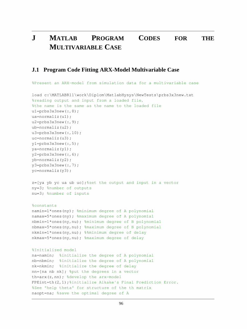
J MATLAB PROGRAM CODES FOR THEMULTIVARIABLE CASE

J.1 Program Code Fitting ARX-Model Multivariable Case

%Present an ARX-model from simulation data for a multivariable case

load c:\MATLABR11\work\Diplom\MatlabHysys\NewTests\prbs3x3new.txt%reading output and input from a loaded file,%the name is the same as the name to the loaded fileu1=prbs3x3new(:,8);ua=normaliz(u1);u2=prbs3x3new(:,9);ub=normaliz(u2);u3=prbs3x3new(:,10);uc=normaliz(u3);y1=prbs3x3new(:,5);ya=normaliz(y1);y2=prbs3x3new(:,6);yb=normaliz(y2);y3=prbs3x3new(:,7);yc=normaliz(y3);

z=[ya yb yc ua ub uc];%set the output and input in a vectorny=3; %number of outputsnu=3; %number of inputs

%constantsnamin=1*ones(ny); %minimum degree of A polynomialnamax=5*ones(ny); %maximum degree of A polynomialnbmin=1*ones(ny,nu); %minimum degree of B polynomialnbmax=5*ones(ny,nu); %maximum degree of B polynomialnkmin=1*ones(ny,nu); %%minimum degree of delaynkmax=5*ones(ny,nu); %maximum degree of delay

%Initialized modelna=namin; %initialize the degree of A polynomialnb=nbmin; %initialize the degree of A polynomialnk=nkmin; %initialize the degree of delaynn=[na nb nk]; %put the degrees in a vectorth=arx(z,nn); %develop the arx-modelFPEint=th(2,1);%initialize Aikake's Final Prediction Error.%See "help theta" for structure of the th matrixnaopt=na; %save the optimal degree of A

96

nbopt=nb; %save the optimal degree of Bnkopt=nk; %save the optimal degree of delayoptparameters=[naopt nbopt nkopt];optFPE=FPEint;optloss_function=th(1,1);opt_th=th;%Check all the combinations of model structure that gives the best%describtion of the processfor i=namin(1,1):1:namax(1,1) for j=nbmin(1,1):1:nbmax(1,1) for k= nkmin(1,1):1:nkmax(1,1) na=i*ones(ny,ny); nb=j*ones(ny,nu); nk=k*ones(ny,nu); nn=[na nb nk]; th=arx(z,nn); %develop the arx-model FPE=th(2,1); %Displays the FPE in the th matrix loss_funciton=th(1,1); if FPE<FPEint %checks the FPE, less value for FPE gives better model FPEint=FPE; %update the FPE value if its less than the past value naopt=na; %save the optimal degree of A nbopt=nb; %save the optimal degree of B nkopt=nk; %save the optimal degree of delay optparameters=[naopt nbopt nkopt]; optFPE=FPE; optloss_function=th(1,1); opt_th=th; end %if end %for end %forend %for

%optimal parameterse=resid(z,opt_th); %compute the residuals and display correlation graphsstdev_e=std(e) %finds the standard devation of the errorvar_e=var(e) %finds the variance of the error

%Display modelparameters and other keyparamters[Aopt,Bopt]=th2arx(opt_th)optFPEoptloss_functionoptparameters

97

J.2 Program Code Recursion of Diophantine in Multivariable Case

function [E_rec,F_rec]= diophantinemulti(A,B,N,ny)%Solves the Diophantine equation, A and B is modelparameters, N is the cost horizon%Uses the recursively method described by Clarcke et. al. in %"Generalized Predictive Control - Part I. The Basic Algorithm"%Automatica. Vol. 23, No.2, pp 137-148, 1987.%Rembember A= I(nyxny)+A1*z(-1)+A2*z(-2)+.....+Ana*z(-na)%where I, A1, A2 ..... Ana are matrixes all of size (ny)x(ny) (ny=number of outputs)

%Initializing E E=eye(ny);

%Initializing FAtilda=[A zeros(ny)]-[zeros(ny) A]; %Atilda=A(1-q^-1)d=size(Atilda);v=[eye(ny) zeros(d(1),d(2)-ny)];Aprime=v-Atilda; %Aprime= 1-AtildaF=Aprime(:,ny+1:size(Aprime,2)); %F=q(1-Atilda)m=size(Aprime,2)-size(F,2);F=[F zeros(ny,m)]; %Size F needs to be equal Atilda= size Aprime

%Saving the E & F for each loop, including the initial valuesE_rec=zeros(N*ny); %Initialize the E that is recordedE_rec(1:ny,1:ny)=E;F_rec=zeros(N*ny,size(F,2));F_rec(1:ny,1:size(F,2))=F; %Initilize F that is recorded

%Recursion loop for Diophantinefor j=2:N r=F(:,1:ny); R=[E r]; %updates the new R value, which takes the first element in F and add in S=F(:,ny+1:end)-r*Atilda(:,ny+1:end); r=[R zeros(ny,N*ny-j*ny)]; % Set R which is E(j+1) so R represent E(j+2) in next loop E_rec(j*ny-(ny-1):j*ny,:)=r; E=R; %Set S which is F(j+1) so S represent F(j+2) in next loop F=[S zeros(ny,size(Atilda,2)-size(S,2))]; F_rec(j*ny-(ny-1):j*ny,:)=F; end

%Erase the last column.

98

%In the calculation the size of F needs to equal the size of Atilda. This adds ny columns.F_rec=F_rec(:,1:size(F_rec,2)-ny);

J.3 Program Code for Initializing

global ny nu yrls urls w A B ypast uopt beta P K nu ny ymean umean ymstore umstore EthInEth PropInProp PropInBot ReboilRatio EthaneFlow PropaneFlow

%Initialize dataupast=zeros(50,1);ypast=zeros(50,1);delta_u=zeros(50,1);yrls=[];urls=[];ymean=[0.9705;0.9623;9.0e-5];umean=[0.4722;0.3611;0.934];ymstore=[];umstore=[];EthInEth=[];PropInProp=[];PropInBot=[];ReboilRatio=[];EthaneFlow=[];PropaneFlow=[];ExitFlag=[];

%Startvalues for the model. Updates by RLS

A=[ 1.0000 0 0 -1.6900 0.2388 0.0595 0.6971 0 1.0000 0 0.0251 -1.9607 0.0451 -0.0256 0 0 1.0000 0.1511 0.0849 -1.6938 -0.1500 -0.2364 -0.0571 0.9633 -0.0429 -0.0797 0.6990];

B=[0 0 0 0.0179 0.0055 -0.0967 0.0032 -0.0023 0 0 0 0.0008 0.0001 0.0037 0.0004 -0.0005 0 0 0 0.0009 0.0009 -0.0235 0.0049 0.0002

0.l1440 -0.0029 -0.0018 -0.0362 0.0011 -0.0004 -0.0148 -0.0005 -0.0005 0.0001 -0.0054 0.0007 0.0002 0.0010 0.0353 0.0003 -0.0007 -0.0132 0.0040 0.0000 0.0005];

99

J.4 Program Code GPC Including QP- Algorithm

global ny nu yrls urls w A B ypast uopt beta P K ny nu ymean umean ymstore umstore EthInEth PropInProp PropInBot ReboilRatio EthaneFlow PropaneFlow

%Algorithm that minimize the cost function subject to constrains%on the control signals and the outputs. Multi-input multi-output case%The file initialize.m needs to be executed before mpcqp.m runs for the first time%The file is executed from VBA

%Declare variablesalfanorm=0.05; %smoothing grade mean values for inputs and outputs%Declare countersj=1;p=1;s=1;i=1;l=1;q=1;r=1;

%Constants, from VBAN1=const(1); %minimum costing horizonNU=const(2); %control horizonN2=const(3); %maximum costing horizonlamda=const(4); %control-weighting sequenseny=const(5); %number of outputsnu=const(6); %number of inputsw1=const(7);%referense trajectory(=setpoint) Mole Fraction Ethane in Ethanew2=const(8); %ref.traj. LV fraction propane in propanew3=const(9); %ref.traj. LV fraction propane in T-2 Bottoms

N=N2-N1+1; %cost horizon

%Declare variablesy=zeros(ny,1); %outputsu=zeros(nu,1); %inputs

%Process data from Hysys%Past outputu(1)=DataFromHysys(1); %Flow ethane. Unit in kmol/su(2)=DataFromHysys(2); %Flow propane. Unit in kmol/su(3)=DataFromHysys(3); %Reboil ratio y(1)=DataFromHysys(4); % Mole Fraction ethane in ethane* stream

100

y(2)=DataFromHysys(5); %LV Fraction propane in propane* streamy(3)=DataFromHysys(6); %LV Fraction propane in T-2 Bottoms* stream

%Normalize data from Hysys because time-series models are developed with%normalized dataynorm=y-ymean;ymean_new=alfanorm*y+(1-alfanorm)*ymean;unorm=u-umean;umean_new=alfanorm*u+(1-alfanorm)*umean;

%Create setpoint vector%length (w) needs to be N*nyw=[];for l=1:N w=[w;w1;w2;w3];end

%Storage of process dataupast=[unorm; upast(1:size(upast,1)-nu)];ypast=[ynorm; ypast(1:size(ypast,1)-ny)];

%Calculate delta u = u(t)-u(t-1). Used in free response for cost function with %delta u as variable. Not generalized for different numbers of nufor s=1:(size(upast,1)-nu)/nu delta_u(nu*s-2)=upast(nu*s-2)-upast(nu*s+nu-2); delta_u(2*s-1)=upast(2*s-1)-upast(2*s+nu-1); delta_u(2*s)=upast(2*s)-upast(2*s+nu);end

%Calculate the Diophantine eq recursivly[E_rec,F_rec]=diophantinemulti(A,B,N,ny);

%Create gconv, used to calculate the G matrix%Not generalized for different numbers of ny!for r=1:N gconv(ny*r-(ny-1),:)=conv(E_rec(ny*r-(ny-1),:),B(ny-2,:)); gconv(ny*r-(ny-2),:)=conv(E_rec(ny*r-(ny-2),:),B(ny-1,:)); gconv(ny*r,:)=conv(E_rec(ny*r,:),B(ny,:));end

%Select diagonals from gconv matrixfor i=1:nu*NU gdiag(:,i)=diag(gconv,i-1);end

101

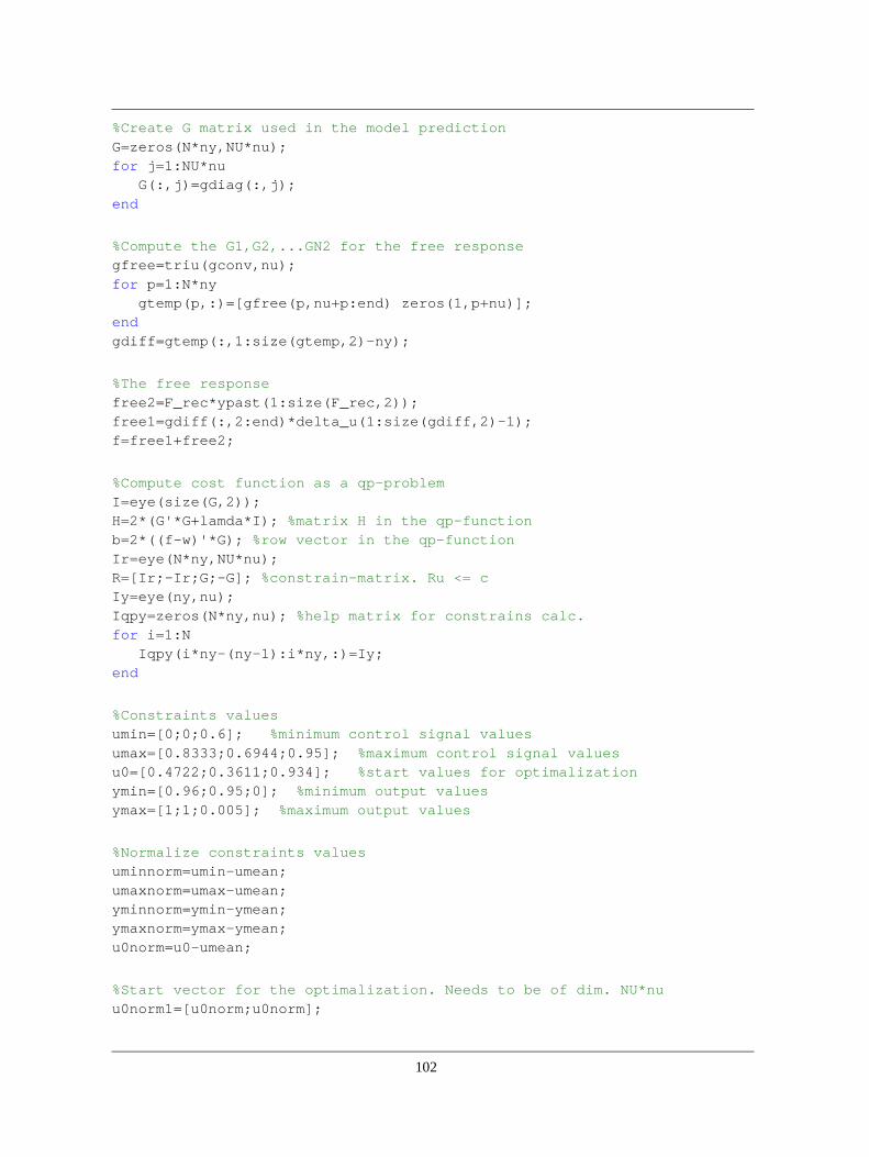
%Create G matrix used in the model predictionG=zeros(N*ny,NU*nu);for j=1:NU*nu G(:,j)=gdiag(:,j);end

%Compute the G1,G2,...GN2 for the free responsegfree=triu(gconv,nu);for p=1:N*ny gtemp(p,:)=[gfree(p,nu+p:end) zeros(1,p+nu)]; endgdiff=gtemp(:,1:size(gtemp,2)-ny);

%The free responsefree2=F_rec*ypast(1:size(F_rec,2));free1=gdiff(:,2:end)*delta_u(1:size(gdiff,2)-1);f=free1+free2;

%Compute cost function as a qp-problemI=eye(size(G,2));H=2*(G'*G+lamda*I); %matrix H in the qp-functionb=2*((f-w)'*G); %row vector in the qp-functionIr=eye(N*ny,NU*nu);R=[Ir;-Ir;G;-G]; %constrain-matrix. Ru <= cIy=eye(ny,nu);Iqpy=zeros(N*ny,nu); %help matrix for constrains calc.for i=1:N Iqpy(i*ny-(ny-1):i*ny,:)=Iy;end

%Constraints valuesumin=[0;0;0.6]; %minimum control signal valuesumax=[0.8333;0.6944;0.95]; %maximum control signal valuesu0=[0.4722;0.3611;0.934]; %start values for optimalizationymin=[0.96;0.95;0]; %minimum output valuesymax=[1;1;0.005]; %maximum output values

%Normalize constraints valuesuminnorm=umin-umean;umaxnorm=umax-umean;yminnorm=ymin-ymean;ymaxnorm=ymax-ymean;u0norm=u0-umean;

%Start vector for the optimalization. Needs to be of dim. NU*nuu0norm1=[u0norm;u0norm];

102

%compute c matrix in constrains eq Ru <= cc=[Iqpy*umaxnorm;-Iqpy*uminnorm;Iqpy*ymaxnorm-f;-Iqpy*yminnorm+f];

%Solving the QP-problem[uoptnorm,fval,exitflag,output]=quadprog(H,b,R,c,[],[],[],[],u0norm1);ExitFlag=[ExitFlag exitflag];

%when the maximum number of iterations was exceeded or the problem is unbounded,%infeasible, or QUADPROG failed to converge with a solution X, %the optimal solution = startpoint to avoid unstability in Hysysif exitflag <=0 uoptnorm=u0norm1;end

%Change optimalized inputs from normalized to realuopt=uoptnorm(1:nu)+umean;

setpoints=[uopt(1:nu)]; %only the first control actions are sended to Hysys

%Scaling setpointsdata. %There is a convertion in Hysys which needs to be %adjusted in Matlabsetpoints(1)=setpoints(1)*1300/10.83;setpoints(2)=setpoints(2)*1190/8.264;setpoints(3)=(setpoints(3)*142.89-71.458)/3600; %reboil ratio need to be to be divided with 3600%because of convertion due to units in Hysys. Reboil ratio is sended to Hysys as a %molar flow in kmol/s

%The RLS part%select inputs and outputs data sended to RLS algorithmrlsdata=[ypast(ny+1:2*ny);unorm]; %call the RLS algorithm[A,B]=adaptmulti(rlsdata);

%Update meanvalues for normalizingymean=ymean_new;umean=umean_new;

%Store ymean and umean to see drifting in processymstore=[ymstore ymean];umstore=[umstore umean];

103

%Store data from processEthInEth=[EthInEth DataFromHysys(4)];PropInProp=[PropInProp DataFromHysys(5)];PropInBot=[PropInBot DataFromHysys(6)];ReboilRatio=[ReboilRatio DataFromHysys(3)];EthaneFlow=[EthaneFlow DataFromHysys(1)];PropaneFlow=[PropaneFlow DataFromHysys(2)];

done=1; %value that tells VBA that Matlab finished the calculations

J.5 Program Code RLS Multivariable Case

function [A,B]=adaptmulti(rlsdata)%Adaptiver based on RLS method in the multivariable case%rlsdata is data from the GPC function

global ny nu yrls urls w A B ypast beta P K

%declare variablesypred=zeros(1,3);

%w is the setpoint trajectory%A and B is modelparamters%ypast is the past mesured values%yrls and urls is vectors the past vector is made from%beta is the parameter estimate in a column vector, P is the covar. matrix%and K is the gain vector

%Save the past datayrls=[rlsdata(1:ny);yrls]; %update the past measurement vectorurls=[rlsdata(ny+1:ny+nu);urls]; %update the past control signals vectori=size(yrls,1); %count how many data the rls algorithm has

%Choose values for the degree of polynomnials and the deadtimen=2; %Degree of the A polynominalm=4; %Degree of the B polynominald=1; %Deadtime

%Test if there is enough data to run RLSif i>=(m+d+ny)*ny %Constants c=1000; %for initializing of the P matrix gama=0.9;%forgetting factor

104

alfa=0.0045; %variance to the error, found from PRBS-data %Initializing of the system beta_init=zeros(n*ny+m*nu,ny); %initialize the beta-vector I=eye(m*nu+n*ny);%identity matrix Pinit=c*I; %initialize the P matrix %vector with past data from measurement and ctrl signal ksi=[yrls(1:ny*n);urls(1+d:nu*m+d)]; %Compute model prediction if i==(m+d+ny)*ny ypred=ksi'*beta_init; %if the loop runs the first time, uses the initlized beta else ypred=ksi'*beta; %if the loop runs 2nd time or more, uses the beta from last run end %Update gain vector if i==(m+d+ny)*ny K=(Pinit*ksi)./(alfa*gama+ksi'*Pinit*ksi); else K=(P*ksi)./(alfa*gama+ksi'*P*ksi); end %Update parameter estimates if i==(m+d+ny)*ny beta=beta_init+K*((yrls(1:ny))'-ypred); %update modelparameter A. The first coeff is always the identity matrix A=[eye(ny);-beta(1:ny*n,1:ny)]'; %updata B. -beta comes from different definition of A and B in RLS and GPC B=[zeros(d*nu,ny);-beta(n*ny+1:n*ny+m*nu,1:ny)]'; else beta=beta+K*((yrls(1:ny))'-ypred); A=[eye(ny);-beta(1:ny*n,1:ny)]'; B=[zeros(d*nu,ny);-beta(n*ny+1:n*ny+m*nu,1:ny)]'; end %Compute covariance matrix for next iteration if i==(m+d+ny)*ny P=(1/gama)*(I-K*ksi')*Pinit; else P=(1/gama)*(I-K*ksi')*P; endelse %else if i>m+d+1 %if not enough data, the ARX-model found from PRBS-data is used %A and B given from the PRBS data

105

A=[ 1.0000 0 0 -1.6900 0.2388 0.0595 0.6971 0 1.0000 0 0.0251 -1.9607 0.0451 -0.0256 0 0 1.0000 0.1511 0.0849 -1.6938 -0.1500 -0.2364 -0.0571 0.9633 -0.0429 -0.0797 0.6990];

B=[0 0 0 0.0179 0.0055 -0.0967 0.0032 -0.0023 0 0 0 0.0008 0.0001 0.0037 0.0004 -0.0005 0 0 0 0.0009 0.0009 -0.0235 0.0049 0.0002

0.l1440 -0.0029 -0.0018 -0.0362 0.0011 -0.0004 -0.0148 -0.0005 -0.0005 0.0001 -0.0054 0.0007 0.0002 0.0010 0.0353 0.0003 -0.0007 -0.0132 0.0040 0.0000 0.0005];

end %end if i>m+d+1

106

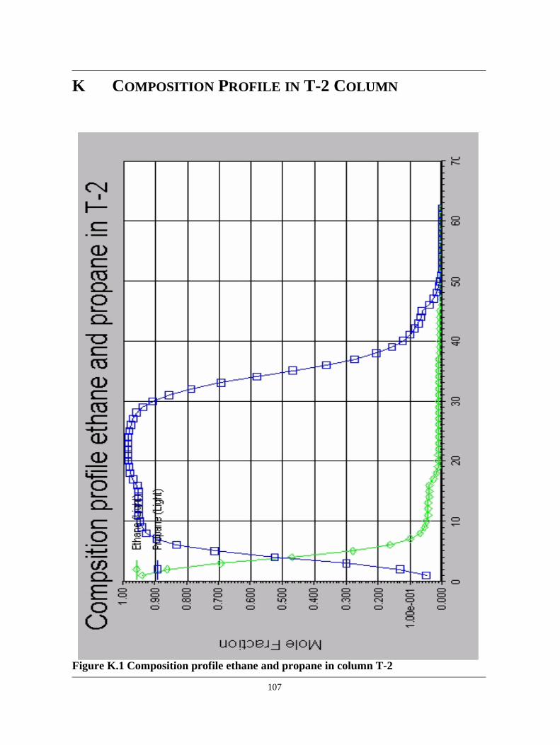
107

K COMPOSITION PROFILE IN T-2 COLUMN

Figure K.1 Composition profile ethane and propane in column T-2

L PROGRAM CODE IN VBA

'**********************************************************'Description: Program that execute HYSYS.Plant simulation'and Matlab algorithm that gives control inputs from'GPC with model-updating based on RLS, and transfer'information between the two programs.'Excel File: MPCControl.xls'Matlab file: mpcqp.m'HYSYS file:B&VSimulationDiam.hsc'Author: Elvira Marie Bergheim'Date: 30.Jan.2001'**********************************************************

'Require all variables to be explicit declaredOption Explicit

'Decleare HYSYS objects'Note: chech HYSYS Type Library and Matlab Aut. Server type'under Tools --> ReferencesPublic HyAppl As ObjectPublic HyCase As SimulationCasePublic HyFlowsheet As FlowsheetPublic HyStreams As StreamsPublic HyQStreams As StreamsPublic Matlab As ObjectPublic ColumnFlowsheet As ColumnFlowsheet

'Declare variablesDim Res As String ' Help variable for Matlab commandsDim DataToMatlab(5, 0) As Double 'array sending data to MatlabDim DataToMatlabIm() As Double 'Imaginary part of DataToMatlabDim Constants(8, 0) As Double 'Array collection constants valuesDim ConstantsIm() As Double 'Imaginary part of ConstantsDim FirstRun As Boolean 'Value True when algorithm runs for the first timeDim MatlabFinish(0, 0) As Double 'tells if Matlab finished the calculationsDim MatlabFinishIm() As Double 'Imaginary part of MatlabFinishDim ToHysysR(2, 0) As Double 'Array containing information to HysysDim ToHysysIm() As Double 'Imaginary part of ToHysysRDim EthController As ControllerDim PropController As ControllerDim BoilupController As ControllerDim T2 As ColumnOpDim CompEth As Variant

108

Dim CompProp As VariantDim CompT2Bot As Variant-----------------------------------------------------------------------Sub MPCControl()

FirstRun = True 'First time the sub is runned

'Connect to Matlab if not already connectedIf Matlab Is Nothing Then Set Matlab = CreateObject("Matlab.Application")End If

'Connect to HYSYS objectsSet HyCase = GetObject("c:\MineDokument\Diplom\Hysys\Dynamics\B&VSimulationDiam105.hsc")'Connect to applications objectSet HyAppl = HyCase.Application'Set an object reference to currently active Hysys simulationSet HyCase = HyAppl.ActiveDocument

'If there is no currently active case then display error messageIf HyCase Is Nothing Then MsgBox "A HYSYS Simulation Case must be open" Exit SubEnd If

'Connect to flowsheet in active simulation caseSet HyFlowsheet = HyCase.Flowsheet'Connect to a collection of all material streamsSet HyStreams = HyFlowsheet.MaterialStreams'Connect to a collection of all energy streamsSet HyQStreams = HyFlowsheet.EnergyStreams'Connect to columnSet T2 = HyFlowsheet.Operations.Item("T-2")

'Connect to operationsSet EthController = HyFlowsheet.Operations.Item("FC-Ethane")Set PropController = HyFlowsheet.Operations.Item("FC-Propane")Set BoilupController = HyFlowsheet.Operations.Item("RC-Boilup")

'Change directoryRes = Matlab.Execute("cd c:\MATLABR11\work\Diplom\MatlabHysys")

'Initialize data

109

If FirstRun Then Res = Matlab.Execute("Initialize") FirstRun = False 'not first time sub is executed anymoreEnd If

'Let the communication between Matlab and Hysys go for a certain timeWhile True' 'Check if Hysys solver is ready If HyAppl.ActiveDocument.Solver.Integrator.IsRunning Then DoEvents Else 'Send GPC constants to Matlab Constants(0, 0) = 1 'Minimimum cost horizon Constants(1, 0) = 2 'Control horizon Constants(2, 0) = 5 'Maximum cost horizon Constants(3, 0) = 1.5 'Lamda (control-weigthing sequence) Constants(4, 0) = 3 'Number of outputs Constants(5, 0) = 3 'Number of inputs Constants(6, 0) = 0.9708 'Setpoint mol fraction ethane in ethane Constants(7, 0) = 0.9622 'Setpint Liquid Volume Fraction propane in propane Constants(8, 0) = 0.000086 ' Setpoint Liquid Volume Fraction propane in T-2 Bottoms

'Send Constant-values to Matlab Call Matlab.PutFullMatrix("const", "base", Constants, ConstantsIm) 'Get data from Hysys that is necessary for control calculation. 'past inputs (u) DataToMatlab(0, 0) = HyStreams.Item("Ethane*").MolarFlow DataToMatlab(1, 0) = HyStreams.Item("Propane*").MolarFlow DataToMatlab(2, 0) = BoilupController.PVValue ' send the smoothed value 'get component fractions CompEth = HyStreams.Item("Ethane*").ComponentMolarFraction.Values CompProp = HyStreams.Item("Propane*").ComponentVolumeFraction.Values CompT2Bot = HyStreams.Item("T-2 Bottoms*").ComponentVolumeFraction.Values 'Past outputs DataToMatlab(3, 0) = CompEth(1) 'Molar Fraction Ethane in Ethane DataToMatlab(4, 0) = CompProp(2) 'LV Fraction Propane in Propane DataToMatlab(5, 0) = CompT2Bot(2) 'LV Fraction Propane in T-2 Bottoms 'Send data to Matlab

110

Call Matlab.PutFullMatrix("DataFromHysys", "base", DataToMatlab,DataToMatlabIm) 'Matlab execute file Res = Matlab.Execute("mpcqp") MatlabFinish(0, 0) = 0 'chech if Matlab fishish algorithm execution While MatlabFinish(0, 0) = 0 Call Matlab.GetFullMatrix("done", "base", MatlabFinish, MatlabFinishIm) DoEvents Wend

'Get setpoints to slavecontrollers for control in Hysys 'Variable "setpoints" from Matlab need to be columnvector Call Matlab.GetFullMatrix("setpoints", "base", ToHysysR, ToHysysIm) 'Give Hysys the new setpoints values from Matlab HyStreams.Item("HelpEthane").MolarFlow.SetValue ToHysysR(0, 0) HyStreams.Item("HelpPropane").MolarFlow.SetValue ToHysysR(1, 0) HyStreams.Item("HelpRatio").MolarFlow.SetValue ToHysysR(2, 0) 'Run model one timestep and stop HyAppl.ActiveDocument.Solver.Integrator.RunFor 2, "minutes" DoEvents End IfWend 'Return to new loop

End Sub

111

M PERFORMANCE OF THE GPC CONTROLLER

M.1 Responses in manipulated variables

Figure M.1 Mole fraction ethane in ethane outlet for different cost and control horizonswhen decreasing ethane molar flow in feed stream

0 20 40 60 80 100 1200.966

0.968

0.97

0.972

0.974

0.976

0.978

Time in minutes

Mol

e fra

ctio

n et

hane

in e

than

e st

ream

N1=1 N2=4 NU=3 lamda=2 N1=1 N2=7 NU=2 lamda=4N1=1 N2=5 NU=3 lamda=3 N1=1 N2=4 NU=3 lamda=3 N1=1 N2=5 NU=2 lamda=3

112

Figure M.2 LV fraction propane in propane outlet for different cost and controlhorizons when decreasing ethane molar flow in feed stream

0 20 40 60 80 100 1200.94

0.945

0.95

0.955

0.96

0.965

0.97

0.975

Time in minutes

LV fr

actio

n pr

opan

e in

pro

pane

stre

am


113

Figure M.3 LV fraction propane in bottom stream for different cost and controlhorizons when decreasing ethane molar flow in feed stream

0 20 40 60 80 100 1200

0.5

1

1.5

2

2.5

3

3.5

4

4.5

5x 10-3

Time in minutes

LV fr

actio

n pr

opan

e in

bot

tom

stre

am


114

M.2 Responses in control signals

Figure M.4 Flowrate ethane outlet for different cost and control horizons whendecreasing ethane molar flow in feed stream.

0 20 40 60 80 100 1200.2

0.3

0.4

0.5

0.6

0.7

0.8

0.9

Time in minutes

Eth

ane

flow

rate

km

ol/s


115

Figure M.5 Flowrate propane outlet for different cost and control horizons whendecreasing ethane molar flow in feed stream

0 20 40 60 80 100 1200.3

0.35

0.4

0.45

0.5

0.55

0.6

0.65

0.7

Time in minutes

Pro

pane

flow

rate

km

ol/s


116

Figure M.6 Reboil ratio for different cost and control horizons when decreasing ethanemolar flowrate in feed stream.

0 20 40 60 80 100 1200.75

0.8

0.85

0.9

0.95

1

Time in minutes

Reb

oil r

atio


117

N PERFORMANCE OF THE BUILT-IN MPC

N.1 Responses manipulated variables

Figure N.1 Mole fraction ethane in ethane outlet for different cost horizon and controlinterval when decreasing ethane molar flow in feed stream

0 20 40 60 80 100 1200.9715

0.9716

0.9716

0.9717

0.9717

0.9718

0.9718

0.9718

0.9719

0.9719

Time in minutes

Eth

ane

in E

than

e [m

ole

fract

ion]

N=5 Ctrl interval 2min N=25 Ctrl interval 2min N=5 Ctrl interval 30 sec

118

Figure N.2 LV fraction propane in propane outlet for different cost horizons andcontrol intervals when decreasing ethane molar flow in feed stream

0 20 40 60 80 100 1200.9646

0.9648

0.965

0.9652

0.9654

0.9656

0.9658

0.966

Time in minutes

Pro

pane

in p

ropa

ne [L

V fr

actio

n]


119

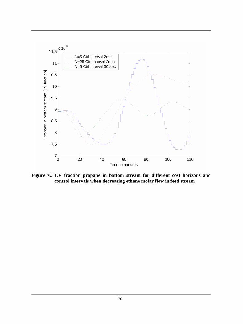
Figure N.3 LV fraction propane in bottom stream for different cost horizons andcontrol intervals when decreasing ethane molar flow in feed stream

0 20 40 60 80 100 1207

7.5

8

8.5

9

9.5

10

10.5

11

11.5x 10-5

Time in minutes

Pro

pane

in b

otto

m s

tream

[LV

frac

tion]


120

N.2 Responses in control signals

Figure N.4 Flowrate ethane outlet for different cost horizons and control intervalswhen decreasing ethane molar flow in feed stream.

0 20 40 60 80 100 1201670

1680

1690

1700

1710

1720

1730

1740

1750

1760

Time in minutes

Eth

ane

flow

[km

ol/h

]


121

Figure N.5 Flowrate propane outlet for different cost horizons and control intervalswhen decreasing ethane molar flow in feed stream

0 20 40 60 80 100 120900

950

1000

1050

1100

1150

1200

1250

1300

1350

Time in minutes

Pro

pane

flow

[km

ol/h

]


122

Figure N.6 Reboil ratio for different cost horizons and control intervals whendecreasing ethane molar flowrate in feed stream.

0 20 40 60 80 100 1200.92

0.925

0.93

0.935

0.94

0.945

0.95

0.955

0.96

Time in minutes

Reb

oil r

atio


123

O COMPARISON OF GPC AND BUILT-IN MPC

O.1 Responses manipulated variables

Figure O.1 Mole fraction ethane in ethane outlet responses for the GPC and the built-in MPC when decreasing ethane molar flow in feed stream

0 20 40 60 80 100 1200.9705

0.971

0.9715

0.972

0.9725

0.973

0.9735

0.974

Time in minutes

Mol

e fra

ctio

n et

hane

in e

than

e st

ream

GPC, N1=1,N2=4,lamda=3Built-in MPC N=25

124

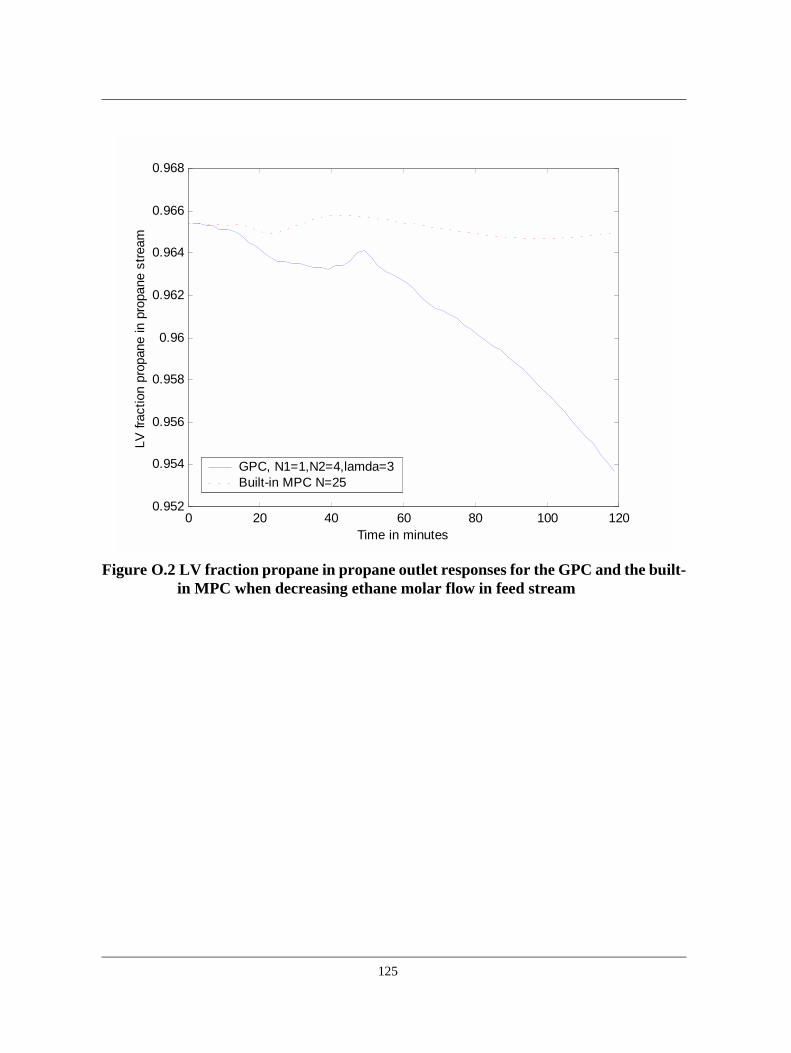
Figure O.2 LV fraction propane in propane outlet responses for the GPC and the built-in MPC when decreasing ethane molar flow in feed stream

0 20 40 60 80 100 1200.952

0.954

0.956

0.958

0.96

0.962

0.964

0.966

0.968

Time in minutes

LV fr

actio

n pr

opan

e in

pro

pane

stre

am


125

Figure O.3 LV fraction propane in bottom stream responses for the GPC and the built-in MPC when decreasing ethane molar flow in feed stream

0 20 40 60 80 100 1200

0.2

0.4

0.6

0.8

1

1.2

1.4x 10-3

Time in minutes

LV fr

actio

n pr

opan

e in

bot

tom

stre

am


126

O.2 Responses in control signals

Figure O.4 Flowrate ethane outlet responses for the GPC and the built-in MPC whendecreasing ethane molar flow in feed stream.

0 20 40 60 80 100 1201550

1600

1650

1700

1750

1800

1850

1900

Time in minutes

Eth

ane

flow

rate

km

ol/h


127

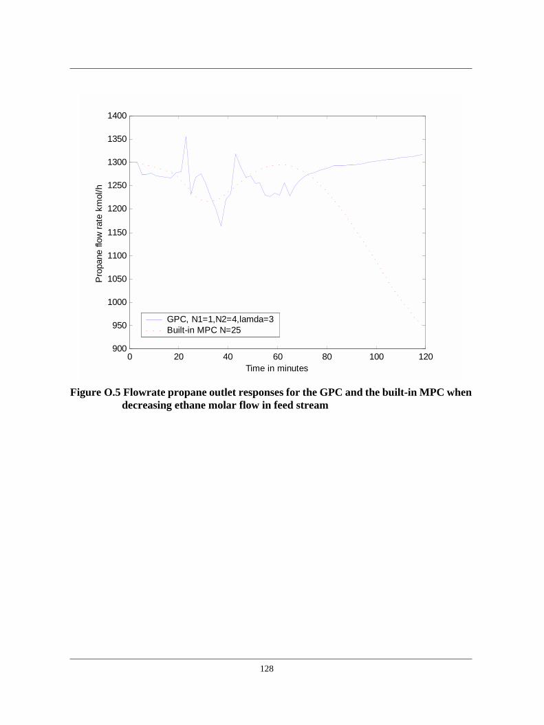
Figure O.5 Flowrate propane outlet responses for the GPC and the built-in MPC whendecreasing ethane molar flow in feed stream

0 20 40 60 80 100 120900

950

1000

1050

1100

1150

1200

1250

1300

1350

1400

Time in minutes

Pro

pane

flow

rate

km

ol/h


128

Figure O.6 Reboil ratio responses for the GPC and the built-in MPC when decreasingethane molar flowrate in feed stream.

0 20 40 60 80 100 1200.86

0.87

0.88

0.89

0.9

0.91

0.92

0.93

0.94

0.95

Time in minutes

Reb

oil r

atio


129

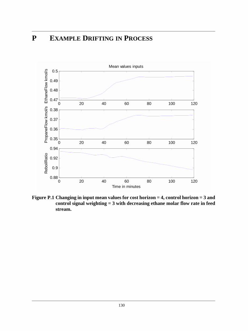
P EXAMPLE DRIFTING IN PROCESS

Figure P.1 Changing in input mean values for cost horizon = 4, control horizon = 3 andcontrol signal weighting = 3 with decreasing ethane molar flow rate in feedstream.

0 20 40 60 80 100 1200.47

0.48

0.49

0.5Mean values inputs

Eth

aneF

low

km

ol/s

0 20 40 60 80 100 1200.35

0.36

0.37

0.38

Pro

pane

Flow

km

ol/s

0 20 40 60 80 100 1200.88

0.9

0.92

0.94

Time in minutes

Reb

oilR

atio

130

Figure P.2 Changing in output mean values for cost horizon = 4, control horizon = 3and control signal weighting = 3 with decreasing ethane molar flow rate infeed stream

0 20 40 60 80 100 1200.97

0.972

0.974Mean values outputs

Eth

mol

frac

0 20 40 60 80 100 1200.95

0.96

0.97

Pro

p LV

frac

0 20 40 60 80 100 1200

2

4

6x 10-4

Pro

p in

Bot

Fra

c

Time in minutes

131

Date post:	11-Dec-2021
Category:	Documents
Upload:	others
View:	2 times
Download:	0 times

NTNU Fakultet for kjemi og biologi

Documents