Al-Qadisiya Journal For Engineering Sciences Vol. 4 No. 3 Year 2011 ۲۳۳ NUMERICAL ANALYSIS OF VAPOR FLOW IN A HORIZONTAL CYLINDERICAL HEAT PIPE Mr. Selah M. Salih Mr. Qahtan A. Abed Mr. Dhafeer M. AL-Shamkhi Automobile Tech. Eng. Dept. Technical College - Najaf Automobile Tech. Eng. Dept. Technical College - Najaf Automobile Tech. Eng. Dept. Technical College - Najaf ABSTRACT The steady two-dimensional flow of a horizontal heat pipe in vapor region is investigated numerically. For study of heat transfer and fluid flow behaviors of the heat pipe, the governing equations in vapor region have been solved using a finite difference method. The numerical results of heat transfer and fluid flow are presented for Reynolds numbers ranging of (Re =4, 10), the Prandtl number taken is (Pr=0.00368), and the pipe dimension is taken to be (L/R =5). The results show that the stream function at the wall increases linearly in the evaporator, decreases linearly in the condenser and is steady in the adiabatic region because of uniform inflow and outflow boundary conditions. Also, it can be seen that as the Reynolds number increases, the pressure distributions shift up without considerable change in their shapes. The numerical analysis have shown that for the low and moderate Reynolds number, the shear stress becomes zero at a point very close to the end of the condenser. For verification of current model, the results of stream function for a heat pipe have been compared with the previous study at the same boundary conditions and a good agreement has been noticed. KEYWORDS—Vapor region; heat pipe; numerical study. . . . . - - - : . ﻓﻲ. . ﺎ ﻟ ﻓ ـﻲ(Re =4, 10) ، (Pr=0.00368) ، ( L/R =5) . " . ، . ﻟ
Transcript
Al-Qadisiya Journal For Engineering Sciences Vol. 4 No. 3 Year 2011
۲۳۳
NUMERICAL ANALYSIS OF VAPOR FLOW IN AHORIZONTAL CYLINDERICAL HEAT PIPE
Mr. Selah M. Salih Mr. Qahtan A. Abed Mr. Dhafeer M. AL-ShamkhiAutomobile Tech. Eng. Dept.
Technical College - NajafAutomobile Tech. Eng. Dept.
Technical College - NajafAutomobile Tech. Eng. Dept.
Technical College - Najaf
ABSTRACT The steady two-dimensional flow of a horizontal heat pipe in vapor region is investigatednumerically. For study of heat transfer and fluid flow behaviors of the heat pipe, the governingequations in vapor region have been solved using a finite difference method. The numerical resultsof heat transfer and fluid flow are presented for Reynolds numbers ranging of (Re =4, 10), thePrandtl number taken is (Pr=0.00368), and the pipe dimension is taken to be (L/R =5). The resultsshow that the stream function at the wall increases linearly in the evaporator, decreases linearly inthe condenser and is steady in the adiabatic region because of uniform inflow and outflow boundaryconditions. Also, it can be seen that as the Reynolds number increases, the pressure distributionsshift up without considerable change in their shapes. The numerical analysis have shown that for thelow and moderate Reynolds number, the shear stress becomes zero at a point very close to the endof the condenser. For verification of current model, the results of stream function for a heat pipehave been compared with the previous study at the same boundary conditions and a good agreementhas been noticed.
INTRODUCTIONThe heat pipe is a vapor-liquid phase-change device that transfers heat from a hot reservoir to
a cold reservoir using capillary forces generated by a wick or porous material and a working fluid.Heat pipes are the most effective passive method of transferring heat available today. Heat pipescan transmit heat at high rates and have a very high thermal conductance.
Heat pipes have been applied to a wide variety of thermal processes and technologies. Heatspipes have been applied in the cooling devices include generators, motors, nuclear, heat collection
Al-Qadisiya Journal For Engineering Sciences Vol. 4 No. 3 Year 2011
۲۳٥
from exhaust gases, solar and geothermal energy. In general, heat pipes have advantages over manytraditional heat-exchange devices, (Doran, 1989).
The vapor flow in heat pipes has been investigated by various authors, (Rajashree andSankara, 1990), (Chan and Faghri, 1995), (Zhu and Vafai, 1999), and (Kim et al, 2003) havepublished many techniques, theories, and experimental investigations of different heat pipestructures. They found the pressure and velocity distributions along the heat pipe depended on thevalue of radial Reynolds numbers.
(Nouri-Borujerdi and Layeghi, 2004) analyzed the vapor flow in concentric annular heatpipe using SIMPLE algorithm and staggered grid scheme. They found the flow and heat for vaporheat pipe was affected by increasing of radial Reynolds numbers.
(Yau, 2007) studied an 8-row thermosyphon-based heat pipe heat exchanger for tropicalbuilding HVAC systems experimentally. This research was an investigation into how the sensibleheat ratio (SHR) of the 8-row HPHE was influenced by each of three key parameters of the inlet airstate, namely, dry-bulb temperature, and relative humidity and air velocity.
(David et al., 2008) design and test of a pressure controlled heat pipe (PCHP), testingshowed that (PCHP) was capable of maintaining a stable evaporator temperature within (0.1K)despite wide swings in heat load and heat sink temperature.
In this paper a numerical model has been used for analysis of vapor flow in heat pipeoperation. The steady state incompressible flow has been solved in cylindrical coordinates in vaporregion. The governing equations have been solved using finite difference with collocated gridscheme. The objective of this paper is study the heat transfer and fluid flow behavior of aconventional heat pipe operation.
MATHEMATICAL MODEL AND GOVERNING EQUATIONSFigure 1 shows the simplified model and the coordinate system of the constant conductance
heat pipe (CCHP) used in the present study. The heat pipe configuration can be divided into threeradial regions, namely, vapor space, wick region and wall region .The working fluid is saturatedwith wick in liquid phase. The power applied to the heater in evaporator causes the liquid in thewick to vaporize. The vapor flows to the condenser section and releases the heat as it condenses.The released heat is rejected through the wall to the ambient. The condensed working fluid in thewick returns to heater section by the capillary force of the wick structure. To analysis the behaviorof flow of fluid and heat through the heat pipe by using continuity, momentum and energyequations as flows.
Heat applied to evaporator section by an external source is conducted through the pipe walland wick structure, where it vaporizes the working fluid. The resulting vapor pressure drives thevapor through the adiabatic section to the condenser, where the vapor condenses and releasing itslatent heat of vaporization to the provided heat sink. The capillary pressure created by the wickstructure, pumps the condensed fluid back to the evaporator. Therefore, the heat pipe cancontinuously transport the latent heat of vaporization from the evaporator to the condenser sections.This process will continue as long as there is sufficient capillary pressure to drive the condensateback to the evaporator.
At the vapor–wick interface, the temperature is assumed to be saturated, corresponding tointerface pressure during heat pipe operation. Axial conduction along the wall and wick is assumednegligible. The steady state two–dimensional incompressible laminar flow with constant viscosity incylindrical (r-x) coordinate, and no heat generation. The governing equations in vapor region arecontinuity, Navier-Stokes and energy equations, (Rajashree and Sankara, 1990), are given asfollows:
0)(1rrv
rxu (1)
Al-Qadisiya Journal For Engineering Sciences Vol. 4 No. 3 Year 2011
۲۳٦
2
212
2
r
uru
rx
uxp
ruv
xuu (2)
2221
22
rv
rv
rv
rxv
rp
rvv
xvu (3)
221
22
rT
rT
rxTK
rTv
xTucp (4)
The radial velocities at liquid-vapor interface, (Borujerdi, 2004), as following:
fgvco
cc
a
fgveo
ee
hLRQ
v
vhLR
Qv
2
0
2(5)
The temperature at the vapor-liquid interface of the evaporator and condenser is calculatedapproximately using Clausius-Clapeyron equation, (Borujerdi, 2004):
)(
)(ln11),(int
satTsatPvTvP
fghR
satT
vrxTT (6)
The boundary conditions for vapor region are as following, (Rajashree and Sankara,1990).At both pipe ends are:
00xT
uv (7)
At pipe centerline the symmetry boundary conditions are:
0&0,0rT
ruv (8)
Pressure gradient at the wall at a particular time is calculated from the momentum equationand it is given by:
ruv
ru
ru
rxp 21
Re2
2
2
(9)
The shear rate is also calculated from the equation:
Al-Qadisiya Journal For Engineering Sciences Vol. 4 No. 3 Year 2011
۲۳۷
ru
Re2 (10)
METHOD OF SOLUTIONThe governing equations are discretized using a finite difference approach and the
equations are solved using upwind difference method with collocated grid scheme as shown inFig.2. For the numerical analysis, it is convenient to use the governing equations in stream functionand vorticity function:
rru (11)
xr (12)
ru
x(13)
Using these and eliminating pressure the governing equations are transformed to
rrrrxr 31
2
2
21
2
2
21 (14)
rrrxrxxrr3
2
2
2
21 (15)
rT
rr
T
x
TrT
xxT
rr1
2
2
2
21 (16)
Now, to make the governing equations form in non-dimensional and the boundaryconditions using the following dimensionless quantities:
vVr
kcppr
sToTT
V
ppVr
vVrVVuu
vrrr
vrxx
v Re;;;2
21*;*
)17(
*;*;*;*;*
By substitution the above dimensionless quantities, in the governing equation of motionyields:
Al-Qadisiya Journal For Engineering Sciences Vol. 4 No. 3 Year 2011
۲۳۸
*
*3*
12*
*2
2*
12*
*2
2*
1* rrrrxr
(18)
2*
*
*
*
*
12*
*2
2*
*2
Re1
*
*
*
*
*
*
*
*
*
1
rrrrxrxxrr(19)
**
12*
2
2*
2
PrRe1
**
*
**
*
*
1rrrxrxxrr
(20)
A finite-difference technique is applied to solve the governing equations. These three
equations Eqs.(18), (19), and (20) are to be solved in a given region subject to the condition that the
values of the stream function, temperature, and the vorticity, or their derivatives, are prescribed on
the boundary of the domain.
Eq.(18) can be approximated using central – difference at the representative interior point
(i , j), then it can be written for regular mesh as:
]2/[)],(ω)())1,(ψ)1,(ψ(
)))(2/(()1,(ψ)1,(ψ),1(ψ),1(ψ[),(ψ2*
2**
2*
2*
2***
**2*
2***
2***
)Δ(Δ)Δ(Δ)Δ(Δ))(Δ())(Δ(
xrjijrrxjijijrrxxjijirjijiji (21)
Also, a central – difference formulation can be used for Eqs.(19), and (20). It is known that
such a formulation may not be satisfactory owing to the loss of diagonal dominance in the sets of
difference equations, with resulting difficulties in convergence when using an iterative procedure.
A forward – backward technique can be introduced to maintain the diagonal dominance
coefficient of (ωi,j) in Eq.(19) and (θi,j) in Eq.(20) which determines the main diagonal elements of
the resulting linear system; this technique is outlined as follows (Najdat,1987):
Set; *j,1-i
*j,1i1 ψψB and *
1-ji,*
1ji,2 ψψB
Then approximate Eq.(19) by:
*
*
*
32*
*2
2*
*2
Re1
*
*
*21
*
*
*22
*
1rrrxrx
B
xr
B
r
Now, if
rff
rf,0B,,,
rff
rf,0 1ji,ji,
1ji,1ji,
1 ΔΔB
if
Al-Qadisiya Journal For Engineering Sciences Vol. 4 No. 3 Year 2011
۲۳۹
ifx
ffxf,0B,,,
xff
xf,0B ji,j,1i
2j,1iji,
2 ΔΔ
where, (f ) refers to ** ,
To assure the diagonal dominance of the coefficient matrix for )ji,*
ji, θω (and)( , which
depends on the sign of ( 1B ) and ( 2B ), Eqs (19) and (20) are expressed in the following difference
forms:
0Bnd,0BFor 21 a
]2
Re)B(B3)(2/[)]1,(ω)(),1(ω)(
),1()ω2
Re()1,()ω32
Re[(),(ω
*
**21
*
*2*2
*2**
2*
2*
**
**22**
*
*2*
*
**12**
* rrx
rrxrxjixjir
jir
rxBrjir
rxrrxBxji
ΔΔΔΔ
ΔΔΔ
(22a)
0Bnd,0BFor 21 a
]2
Re)B(B3)(2/[)]1,(ω)(),1(ω)(
),1()ω2
Re()1,()ω32
Re[(),(ω
*
**21
*
*2*2
*2**
2*
2*
**
**22**
*
*2*
*
**12**
* rrx
rrxrxjixjir
jir
rxBrjir
rxrrxBxji
ΔΔΔΔ
ΔΔΔ
(22b)
0Bnd,0BFor 21 a
]2
Re)B(B3)(2/[)]1,(ω)(),1(ω)(
),1()ω2
Re()1,()ω32
Re[(),(ω
*
**12
*
*2*2
*2**
2*
2*
**
**22**
*
*2*
*
**12**
* rrx
rrxrxjixjir
jir
rxBrjir
rxrrxBxji
ΔΔΔΔ
ΔΔΔ
(22c)
0Bnd,0BFor 21 a
]2
Re)BB-(3)(2/[)]1,(ω)(),1(ω)(
),1()ω2
Re()1,()ω32
Re[(),(ω
*
**21
*
*2*2
*2**
2*
2*
**
**22**
*
*2*
*
**12**
* rrx
rrxrxjixjir
jir
rxBrjir
rxrrxBxji
ΔΔΔΔ
ΔΔΔ
(22d)
Dimensionless energy equation by using upwind finite difference:
Al-Qadisiya Journal For Engineering Sciences Vol. 4 No. 3 Year 2011
۲٤۰
0Bnd,0BFor 21 a
]2
PrRe)B(B)(2/[)]1,()(),1()(
),1()2
PrRe()1,()2
PrRe[(),(
*
**21
*
*2*2
*2**
2*
2*
**
**22**
*
*2*
*
**12**
* rrx
rrxrxjixjir
jirrxBrji
rrx
rrxBxji
ΔΔΔΔ
ΔΔΔ
(23a)
0Bnd,0BFor 21 a
]2
PrRe)B(B)(2/[)]1,()(),1()(
),1()2
PrRe()1,()2
PrRe[(),(
*
**21
*
*2*2
*2**
2*
2*
**
**22**
*
*2*
*
**12**
* rrx
rrxrxjixjir
jirrxBrji
rrx
rrxBxji
ΔΔΔΔ
ΔΔΔ
(23b)
0Bnd,0BFor 21 a
]2
PrRe)B(B)(2/[)]1,()(),1()(
),1()2
PrRe()1,()2
PrRe[(),(
*
**12
*
*2*2
*2**
2*
2*
**
**22**
*
*2*
*
**12**
* rrx
rrxrxjixjir
jirrxBrji
rrx
rrxBxji
ΔΔΔΔ
ΔΔΔ
(23c)
0Bnd,0BFor 21 a
]2
PrRe)B(-B)(2/[)]1,()(),1()(
),1()2
PrRe()1,()2
PrRe[(),(
*
**21
*
*2*2
*2**
2*
2*
**
**22**
*
*2*
*
**12**
* rrx
rrxrxjixjir
jirrxBrji
rrx
rrxBxji
ΔΔΔΔ
ΔΔΔ
(23d)
The corresponding boundary conditions at both ends of the heat pipe which are the no slipcondition for the velocity and adiabatic condition for temperature.
0*
;0*,*;*
)24(
0*
;0*,0*;0*
xr
vrL
vrLxat
xrxat
At the centerline, the symmetry conditions are applied.
Al-Qadisiya Journal For Engineering Sciences Vol. 4 No. 3 Year 2011
۲٤۱
)25(0*
;00,**;0* rxrat
At the vapor –wick interface:
)26(*20*1,**;1* dx
fghveLQvr
xvrxrat
According to the coordinate system shown in figure 1, stream function *,** rx is
negative in evaporator and positive in the condenser while in adiabatic regain is zero, (Borujerdi,2004) .
)(
)(ln1
11,*
satTsatPvTvP
fghR
satTTT
x
so
(27)
The solution procedure of the discredited equations is based on a line-by-line iterationmethod in the axial and radial directions using FORTRAN program. The sequence of numericalsteps based on upwind difference is as follows:1. Initialize the velocity, pressure, shear rate and temperature fields( ,*,*,*,* Pvu ).
2. Solve Eqs.(11) and (12) for u and v.3. Solve Eq. (9) for P.4. Solve Eq. (10) for τ.5. Solve Eq. (20) for θ .6. Check Eq. (28) for convergence, if it is satisfied, calculations will be ended. Otherwise, replace( ,*,*,*,* Pvu ) and return to step (2) and repeat the above procedure until convergence is
achieved.The accuracy of the numerical solution is checked first by summation of the absolute value
of the relative errors should be equal or less than (10-4). Second, the spot value should approach aconstant value. The relative error (Err) in the numerical procedure is defined as, (Borujerdi, 2004):
41011
cells nnn
Err (28)
where superscript ( n ) refers to the previous iteration and term ( )refers to ( =u, v, P, τ, θ).A cylindrical heat pipe with water as working fluid is selected, in which the length of the
evaporator is the same as the length of the condenser and a comparatively long adiabatic section isconsidered. The pipe dimensions are taken to be (L/R =5), increment in space coordinates are(Δx=0.05) and (Δr =0.1). The computation is done for a mesh (101×11), Reynolds number (4 and10), and the Prandtl number taken is (Pr=0.00368). In the present analysis, the axial conductionalong the heat pipe wall is neglected. The evaporator is maintained at constant temperature over itsentire length and the condenser is cooled uniformly and is also kept at constant temperature.
Al-Qadisiya Journal For Engineering Sciences Vol. 4 No. 3 Year 2011
۲٤۲
RESULTS AND DISCUSSIONA computer program has been developed for predicting the stream function, radial and axial
velocities, and temperature, pressure, and shear rate fields of vapor flow along the copper-waterheat pipe. Using this program, a symmetric heat addition and rejection conditions are observed, asshown in Fig.1.
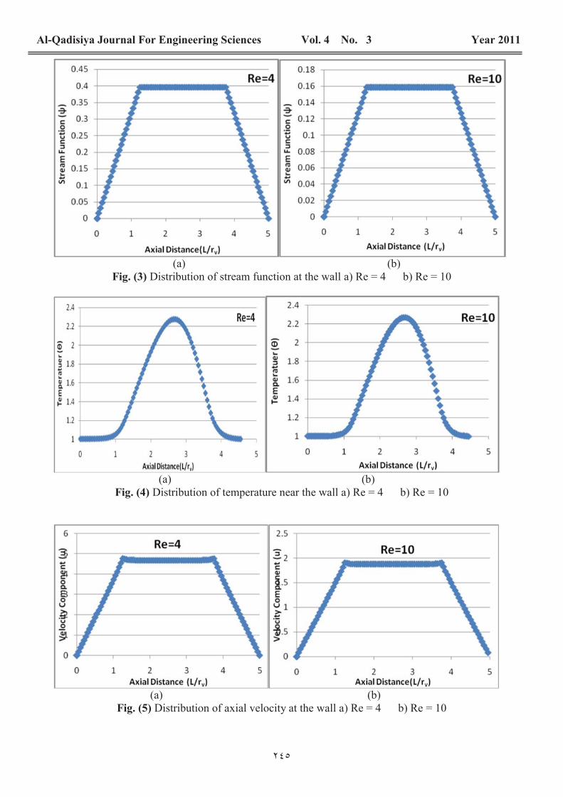
The stream function Fig.3 at the wall increases linearly in the evaporator, decreases linearlyin the condenser and is steady in the adiabatic region because of uniform inflow and outflowboundary conditions. From the axial variation of temperature graph Fig.4 it is found that thetemperature increases in the evaporator section, decreases in the condenser section, and theminimum temperature occurs in the condenser region. As the temperature in the evaporatorincreases, the vapor density in this section also increases and molecular mean free path becomessmall compared to the vapor core diameter. Because of the vapor condenses and releasing its latentheat of vaporization to the provided heat sink.
When the Reynolds number is small, the streamlines are in the direction of increasing axialdistance and the axial velocity component is positive everywhere with a transition to zero valueoccurring in a thin layer at the walls which is observed from Fig.5. The axial velocity profilebecomes fully developed in a short distance and stays parabolic all along the length of the heat pipe.Because of the length of evaporator and condenser section is equal, and then the two quantities ofevaporation and condensation of vapor are equal.
Also the radial velocity is negative in the evaporator section, zero in adiabatic section andpositive in the condenser section, because of the flow direction is assumed negative of downwardand positive of upward direction, as shown in Fig.6.
Figure 7 illustrates the pressure distribution along the heat pipe space centerline for variousReynolds numbers. It can be seen that as the Reynolds number increases, the pressure distributionsshift up without considerable change in their overall shapes. As the Reynolds number increases thepressure in the condenser section is more recovered. The pressure distribution in the adiabaticsection is a straight line similar to poiseuille flow results, while the profiles in the evaporator andcondenser section demonstrate the effects of pressure head absorbed or created by evaporation orcondensation, Due to the small pressure drop along the heat pipe at evaporator and condensersections.
The shear rate as shown in Fig.8 is found to be symmetric. Similar pattern follows forpressure distribution and the decrease in vapor pressure occurs smoothly in evaporator section,remains steady in the adiabatic section and then increases smoothly in the condenser sectionbecause of uniform inflow and outflow boundary conditions are equal.
The numerical analysis have shown that for the Reynolds number (Re=4, 10), the shearstress becomes zero at a point very close to the end of the condenser. However, as the Reynoldsnumber increases, the flow reversal point moves backward toward the adiabatic section. Under thiscondition, the reversed flow region extends from the flow reversal point to the end of the condenser.
To verify our numerical solution we have recovered the heat pipe. A computer code,developed in the present work based on the FORTRAN language, has been validated using theresults based on similar problem with those reported by (Rajashree and Sankara, 1990), as shownin Fig.9 shows stream function comparison with previous study. This demonstrates that the presentnumerical analysis a good agreement for predicting the stream function distribution at Reynoldsnumber (Re=4).
CONCLUSION A numerical study is investigated the flow, temperature, velocity, pressure, and shear stressdistributions for a horizontal heat pipe based on the obtained results in the present study, findingare:
1- At low and moderate Reynolds numbers, the present analysis predicts very small vaportemperature drop along the heat pipe. Due to the small pressure drop along the heat pipe.
Al-Qadisiya Journal For Engineering Sciences Vol. 4 No. 3 Year 2011
۲٤۳
2- The results show the stream function at the wall increases linearly in the evaporator,decreases linearly in the condenser and is steady in the adiabatic region because of uniforminflow and outflow boundary conditions.
3- Also, it can be seen that as the Reynolds number increases, the pressure distributions shiftup without considerable change in their shapes.
4- The numerical analysis have shown that for the low and moderate Reynolds number, theshear stress becomes zero at a point very close to the end of the condenser.
5- The results have been compared with the available numerical data which have been done inthe literature and have shown a good agreement.
REFERENCES [1] F.Doran, 1989, “Heat pipe research and development in the Americas,” Heat Recovery Systemsand CHP, Vol.9, pp.67-100.
[2] R.Rajashree and K. Sankara, 1990, ‘‘ A numerical Study of the Performance of Heat Pipe,’’Indian J. pure appl. Math, 21(1), pp: 95-108.
[3] M. M. Chan and A. Faghri, 1995, “An Analysis of The Vapor Flow and Heat ConductionThrough The Liquid Wick and Pipe Wall in a Heat Pipe With Single or Multiple Heat Sources,” Int.J. Heat Mass Transfer, Vol. 33, No. 9, pp. 194.
[4] N. Zhu and K. Vafai, 1999, “Analysis of Cylindrical Heat Pipe Incorporating the Effect ofLiquid-Vapor Coupling and Non-Darcian Transport-A Closed form Solution,” Int. J. Heat MassTransfer, Vol. 42, pp. 3405- 3418.
[5] S. J. Kim, J. K. Seo and K. H. Do, 2003, “Analytical and Experimental Investigation on theOperational Characteristics and Thermal Optimization of a Miniature Heat Pipe with a GroovedWick Structure,” Int. J. Heat Mass Transfer, Vol. 46, pp. 2051-2063.
[6] A. Nouri-Borujerdi and M. Layeghi, , 2004, “Numerical Analysis of Vapour Flow in ConcentricAnnular Heat Pipes,” Transaction of ASME: Journal of Heat Transfer, Vol. 126, pp. 442-448.
[7] Y. H. Yau , 2007, “Application of a heat pipe heat exchanger to dehumidification enhancementin a HVAC system for tropical climates – a baseline performance characteristics study,”International Journal of Thermal sciences , Vol. 46, pp.164 -171.[8] David B. Sarraf, Sanjida Tamanna, and Peter M. Dussinger, 2008, “pressure controlled heatpipe for precise temperature control,” Space Technology and Applications International, AmericanInstitute of Physics, pp. 3-11.
[9] A. Nouri-Borujerdi , 2004 “A Numerical Analysis of Vapor Flow in Concentric Annular HeatPipes,” Transaction of ASME: Journal of Fluids Engineering, Vol. 126, pp.442- 448.