1

Numerical and experimental analysis of a cantilever

beam: A laboratory project to introduce geometric

nonlinearity in Mechanics of Materials

Tarsicio Beléndez (1) and Augusto Beléndez (2)

(1) Departamento de Ciencia y Tecnología de los Materiales.

Universidad Miguel Hernández de Elche.

Avda. del Ferrocarril, s/n. E-03202. Elche (Alicante). SPAIN

(2) Departamento de Física, Ingeniería de Sistemas y Teoría de la Señal.

Universidad de Alicante. Apartado 99. E-03080 Alicante. SPAIN

Corresponding author: A. Beléndez

Phone: +34-6-5903651

Fax: +34-6-5903464

E-mail: augusto@disc.ua.es

2

ABSTRACT

The classical problem of deflection of a cantilever beam of linear elastic material,

under the action of an uniformly distributed load along ist length (its own weight) and

an external vertical concentrated load at the free end, is experimentally and

numerically analyzed. We present the differential equation governing the behaviour of

this system and show that this equation, although straightforward in appearance, is in

fact rather difficult to solve due to the presence of a non-linear term. The experiment

described in this paper is an easy way to introduce students to the concept of

geometric nonlinearity in mechanics of materials. The ANSYS program is used to

numerically evaluate the system and calculate Young’s modulus of the beam material.

Finally, we compare the numerical results with the experimental ones obtained in the

laboratory.

3

SUMMARY OF THE EDUCATIONAL ASPECTS OF THIS PAPER

1. This paper proposes the introduction of the concept of geometric nonlinearity in

an introductory mechanics of materials course by means of the analysis of a

simple laboratory experiment on the bending of a cantilever beam.

2. The experimental set-up is composed of very simple elements and only easy

experimental measurements -lengths and masses- need be made.

3. The differential equation governing the behaviour of this system is derived

without difficulty and by analyzing this equation it is possible to show that,

although straightforward in appearance, it is in fact rather difficult to solve due to

the presence of a non-linear term.

4. The numerical analysis of the beam is made using a personal computer with the

help of the ANSYS program, and the way in which the modulus of elasticity of

the beam material can be obtained is very illustrative for students.

5. The behavior of the cantilever beam experimentally analyzed is nonlinear except

for an external load F = 0. This enables students to understand when the linear

theory, that is a first order approximation of the general case, can be applied and

when it is necessary to consider the more general nonlinear theory.

6. The experiment described in this paper provides students with not only an

understanding of geometric nonlinearity but also a better understanding of the

basic concepts of mechanics of materials. Additionally, the experiment enables

students to apply these well-understood concepts to a practical problem.

4

1.- INTRODUCTION

Beams are common elements of many architectural, civil and mechanical engineering

structures [1-5] and the study of the bending of straight beams forms an important and

essential part of the study of the broad field of mechanics of materials and structural

mechanics. All undergraduate courses on these topics include the analysis of the

bending of beams, but only small deflections of the beam are usually considered. In

such as case, the differential equation that governs the behavior of the beam is linear

and can be easily solved.

However, we believe that the motivation of students can be enhanced if some

of the problems analyzed in more specialized books on mechanics of materials or

structural mechanics are included in the undergraduate courses on these topics.

However, it is evident that these advanced problems cannot be presented to

undergraduate students in the same way as is done in the specialized monographs [6].

As we will discuss in this paper, it is possible to introduce the concept of geometric

nonlinearity by studying a very simple experiment that students can easily analyze in

the laboratory, that is, the bending of a cantilever beam. The mathematical treatment

of the equilibrium of this system does not involve great difficulty [5]. Nevertheless,

unless small deflections are considered, an analytical solution does not exist, since for

large deflections a differential equation with a non-linear term must be solved. The

problem is said to involve geometric non-linearity [6-8].

The purpose of this paper is to analyze a simple laboratory experiment in order

to introduce the concept of geometric nonlinearity in a course on mechanics or

strength of materials. This type of nonlinearity is related to the nonlinear behavior of

deformable bodies, such as beams, plates and shells, when the relationship between

5

the extensional strains and shear strains, on the one hand, and the displacement, on the

other, is taken to be nonlinear, resulting in nonlinear strain-displacement relations. As

a consequence of this fact, the differential equations governing this system will turn

out to be nonlinear. This is true in spite of the fact that the relationship between

curvatures and displacements is assumed to be linear. The experiment will allow

students to explore the deflections of a loaded cantilever beam and to observe in a

simple way the nonlinear behavior of the beam.

We will consider a geometrically nonlinear beam problem by numerically and

experimentally analyzing the large deflections of a cantilever beam of linear elastic

material, under the action of an external vertical tip load at the free end and a

uniformly distributed load along its length (its own weight). Under the action of these

external loads, the beam deflects into a curve called the elastic curve or elastica. If the

thickness of the cantilever is small compared to its length, the theory of elastica

adequately describes the large, non-linear displacements due to the external loads.

The experimental analysis is completed with a numerical analysis of the

system using the ANSYS program, a comprehensive finite element package, which

enables students to solve the nonlinear differential equation and to obtain the modulus

of elasticity of the beam material. To do this, students must fit the experimental

results of the vertical displacement at the free end to the numerically calculated values

for different values of the modulus of elasticity or Young’s modulus by minimizing

the sum of the mean square root. Using the modulus of elasticity previously obtained,

and with the help of the ANSYS program [9], students can obtain the elastic curves of

the cantilever beam for different external loads and compare these curves with the

experimental ones. ANSYS is a finite element modelling and analysis tool. It can be

used to analyze complex problems in mechanical structures, thermal processes,

6

computational fluid dynamics, magnetics, electrical fields, just to mention some of its

applications. ANSYS provides a rich graphics capability that can be used to display

results of analysis on a high-resolution graphics workstation.

In recent years, personal computers have become everyday tools of

engineering students [10], who are familiar with programs such as Mathematica,

Matlab or ANSYS, which also have student versions. Thanks to the use of computers

and commercial software, students can now gain additional insight into fundamental

concepts by numerical experimentation and visualization [10] and are able to solve

more complex problems. Use of the ANSYS program to carry out numerical

experiments in mechanics of materials has been analyzed, for example, by Moaveni

[10]. In addition, since 1998 in the Miguel Hernández University (Spain), one of the

authors of this paper (T.B.) has proposed numerical experiments using the ANSYS

program for students of an introductory level course on strength of materials (second-

year), an advanced mechanics of materials course for materials engineers (fourth-

year) and a structural analysis course (fifth-year), in a similar way to that described in

Moaveni’s paper. However, in this study we supplement the numerical simulations

performed using the ANSYS program with laboratory experiments, thereby providing

the students with a more comprehensive view of the problem analyzed.

2.- EXPERIMENTAL SET-UP

In the laboratory it is possible to design simple experiments in order to analyze the

deflection of a cantilever beam with a tip load applied at the end free. For example,

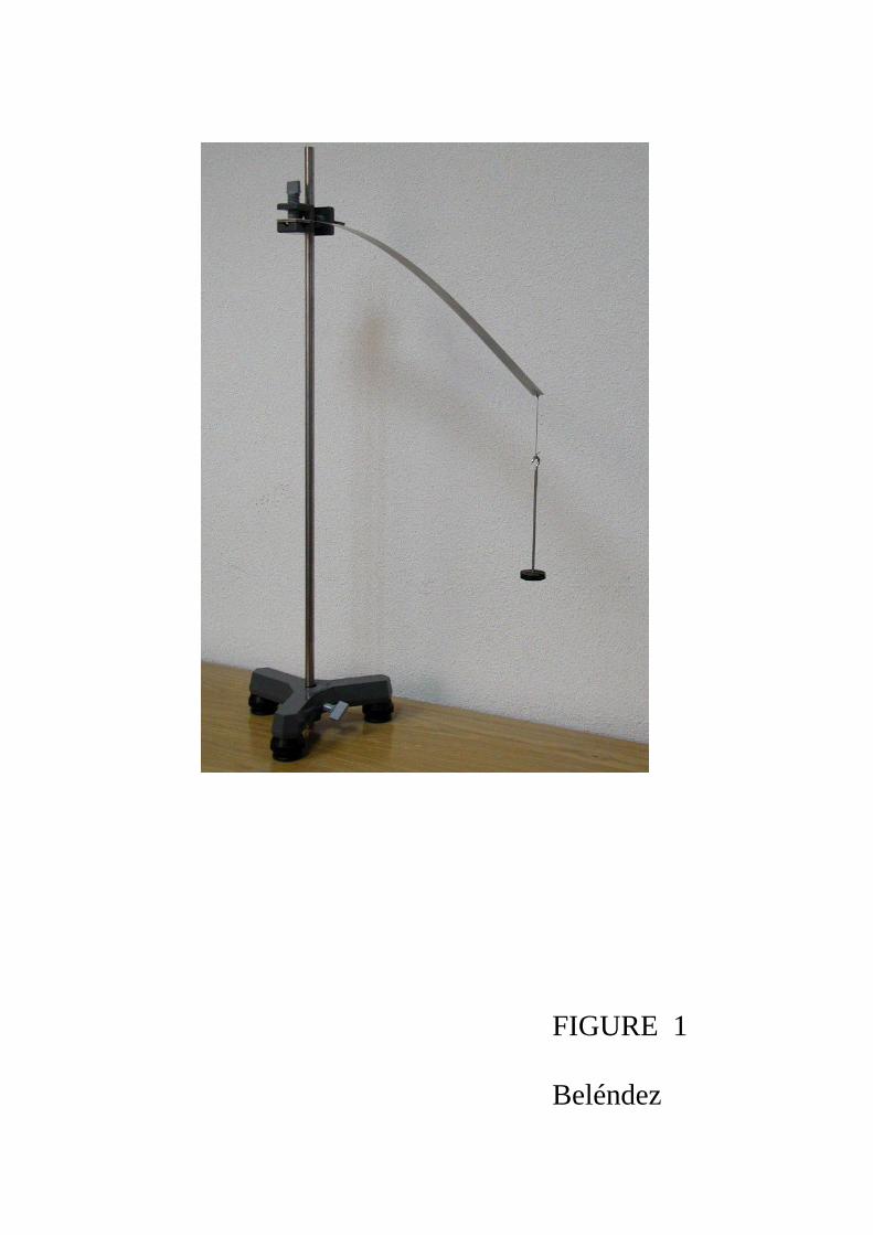
Figure 1 shows a photograph of a system made up of a flexible steel beam of

7

rectangular cross-section built-in at one end and loaded at the free end with a mass.

The beam is fixed to a vertical stand rod by means of a multi-clamp using two small

metallic pieces, which provide a better support (Figure 2). The length of the beam is L

= 0.40 m and it has a uniform rectangular cross-section of width b = 0.025 m and

height h = 0.0004 m. The weight of the beam and the value of the load uniformly

distributed over its entire length are W = 0.3032 N and w = W/L = 0.758 N/m,

respectively.

With this experimental set-up the students can, for instance, determine the

vertical deflection of the end free as a function of the applied load, or the shape the

beam adopts under the action of that force, by using vertical and horizontal rulers as

can be seen in Figure 3. This figure shows the procedure followed to obtain the

experimental measurements of the elastic curve of the beam as well as of the

horizontal and vertical displacements at the free end. The students can relate these

measurements to geometric parameters of the beam (its length and the moment of

inertia of its rectangular cross-section), as well as to the material of which it is made

(using Young’s modulus). This system is made up of very simple elements and only

easy experimental measurements (basically lengths and masses) need be made. In

addition, mathematical treatment of the equilibrium of the system does not involve

great difficulty [11], however for large deflections a differential equation with a non-

linear term must be solved and the problem involves geometrical non-linearity [6-8].

8

3.- THEORETICAL ANALYSIS

Let us consider the case of a long, thin, cantilever beam of uniform rectangular cross

section made of a linear elastic material, whose weight is W, subjected to a tip load F

as shown in Figures 4 and 5. In this study, we assume that the beam is non-extensible

and the strains remain small. Firstly, we assume that Bernoulli-Euler’s hypothesis is

valid, i. e., plane cross-sections which are perpendicular to the neutral axis before

deformation remain plane and perpendicular to the neutral axis after deformation.

Next, we also assume that the plane-sections do not change their shape or area.

The Bernoulli-Euler bending moment-curvature relationship for a uniform-

section rectangular beam of linear elastic material can be written as follows:

κEIM = (1)

where E is the Young’s modulus of the material, M and κ are the bending moment

and the curvature at any point of the beam, respectively, and I is the moment of inertia

(the second moment of area) of the beam cross-section about the neutral axis [3-6].

The product EI, which depends on the type of material and the geometrical

characteristics of the cross-section of the beam, is known as the flexural rigidity.

The moment of inertia of the cross section is given by the equation [1]:

3

12

1hbI = (2)

and its value for the cantilever beam experimentally analyzed is I = 1.333 x 10-13 m4.

9

Equation (1) -which involves the bending moment, M- governs the deflections

of uniform rectangular cantilever beams made of linear type material under general

loading conditions. Differentiating equation (1) once with respect to s, we can obtain

the equation that governs large deflections of a uniform rectangular cantilever beam:

s

M

EIs d

d1

d

d=

κ (3)

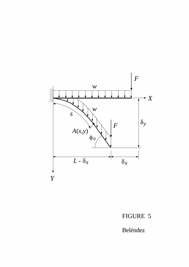
In Figures 4 and 5, δx and δy are the horizontal and vertical displacements at

the free end, respectively, and ϕ0 takes into account the maximum slope of the beam.

We take the origin of the Cartesian coordinate system at the fixed end of the beam and

let (x,y) be the coordinates of point A, and s the arc length of the beam between the

fixed end and point A. The bending moment M at a point A with Cartesian coordinates

(x,y) can be easily calculated from the equation:

[ ] )(d)()()( xLFusxuxwsM x

L

s−−+−= ∫ δ (4)

where L – δx – x is the distance from the section of the beam at a point A to the free

end where force F is applied, and u is a dummy variable of s.

Differentiating equation (4) once with respect to s and recognizing that cosϕ =

dx/ds:

ϕϕ coscos)(d

dFsLw

s

M−−−= (5)

Using equation (5), we can write equation (2) as follows:

10

[ ] )(cos)(1

d

)(d2

2

sFsLwEIs

sϕ

ϕ+−−= (6)

where we have taken into account the relation between κ and ϕ:

sd

dϕκ = (7)

Equation (6) is the non-linear differential equation that governs the deflections

of a cantilever beam made of a linear material under the action of a uniformly

distributed load and a vertical concentrated load at the free end.

The boundary conditions of equation (6) are:

ϕ(0) = 0 (8)

0d

d=

=Lss

ϕ (9)

Taking into account that cosϕ = dx/ds and sinϕ = dy/ds, the x and y

coordinates of any point of the elastic curve of the cantilever beam are found as

follows:

∫=s

sssx0

d)(cos)( ϕ (10)

∫=s

sssy0

d)(sin)( ϕ (11)

11

From Figure 5, it is easy to see that the horizontal and vertical displacements

at the free end can be obtained from equations (10) and (11) for s = L:

)(LxLx −=δ (12)

)(Lyy =δ (13)

4.- NUMERICAL AND EXPERIMENTAL RESULTS

We shall now study the large deflections of a cantilever beam using the ANSYS

program, a comprehensive finite element package. We use the ANSYS/Structural

package that simulates both the linear and nonlinear effects of structural models in a

static or a dynamic enviroment. Firstly we have to obtain the Young’s modulus of the

material. To do this, we obtain experimentally the values of the vertical displacements

at the free end, δy, for different values of the concentrated load F applied at the free

end of the beam. We consider seven values for F: 0, 0.098, 0.196, 0.294, 0.392, 0.490

and 0.588 N and we obtain the theoretical value of δy for different values of E around

the value of E = 200 GPa (the typical value of Young’s modulus for steel) using the

ANSYS program. We obtain the value of Young’s modulus E by comparing the

experimentally measured displacements at the free end δy,exp(Fj), where j = 1, 2, …, J;

J being the number of different external loads F considered (in our analysis J = 7),

with the numerically calculated displacements δy(E,Fj). We obtain the value of E for

which the sum of the mean square root χ2 is minimum, where χ2 is given by the

following equation:

12

[ ]∑=

−=J

j

jexpyjy FFEE1

2,

2 )(),()( δδχ (14)

In Figure 6 we have plotted the calculated values of χ2 as a function of E. The

value of Young’s modulus that minimizes the quantity χ2 is E = 200 GPa, which

implies that the flexural rigidity is EI = 0.02667 Nm2.

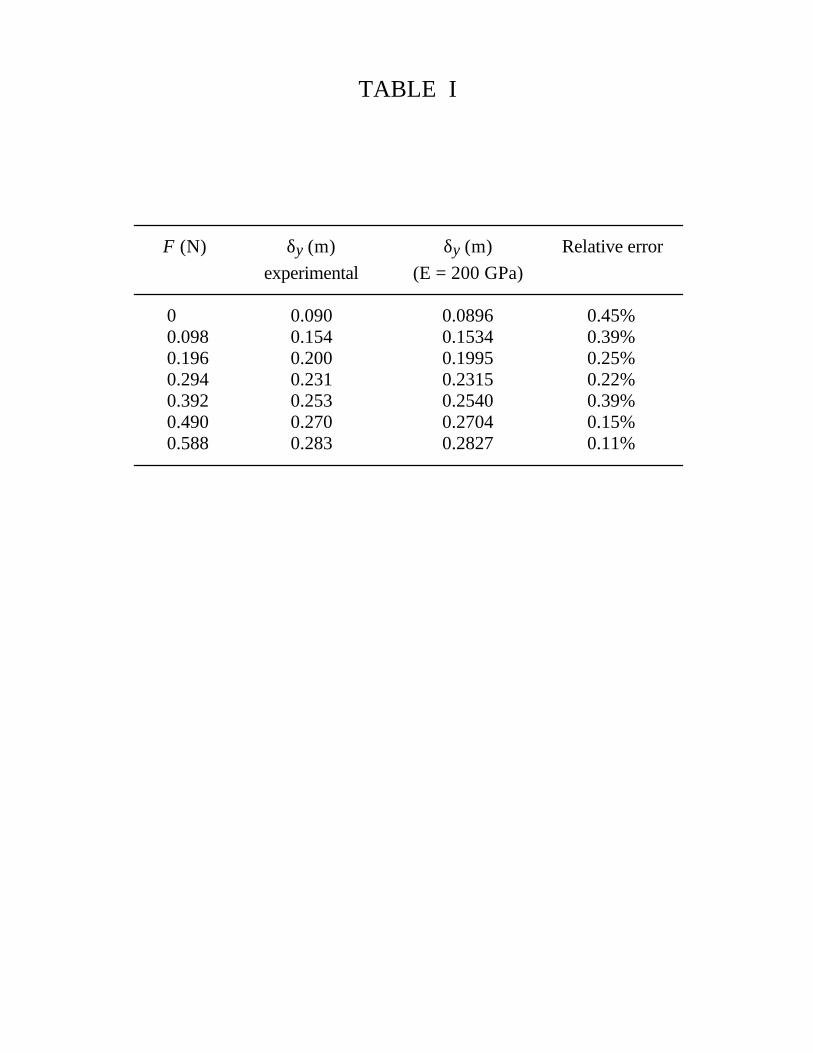
Table I shows the experimental values of δy as a function of the applied load F

together with the values of δy calculated numerically with the aid of the ANSYS

program. We also included the relative error of the values of δy calculated

theoretically as compared with the values measured experimentally.

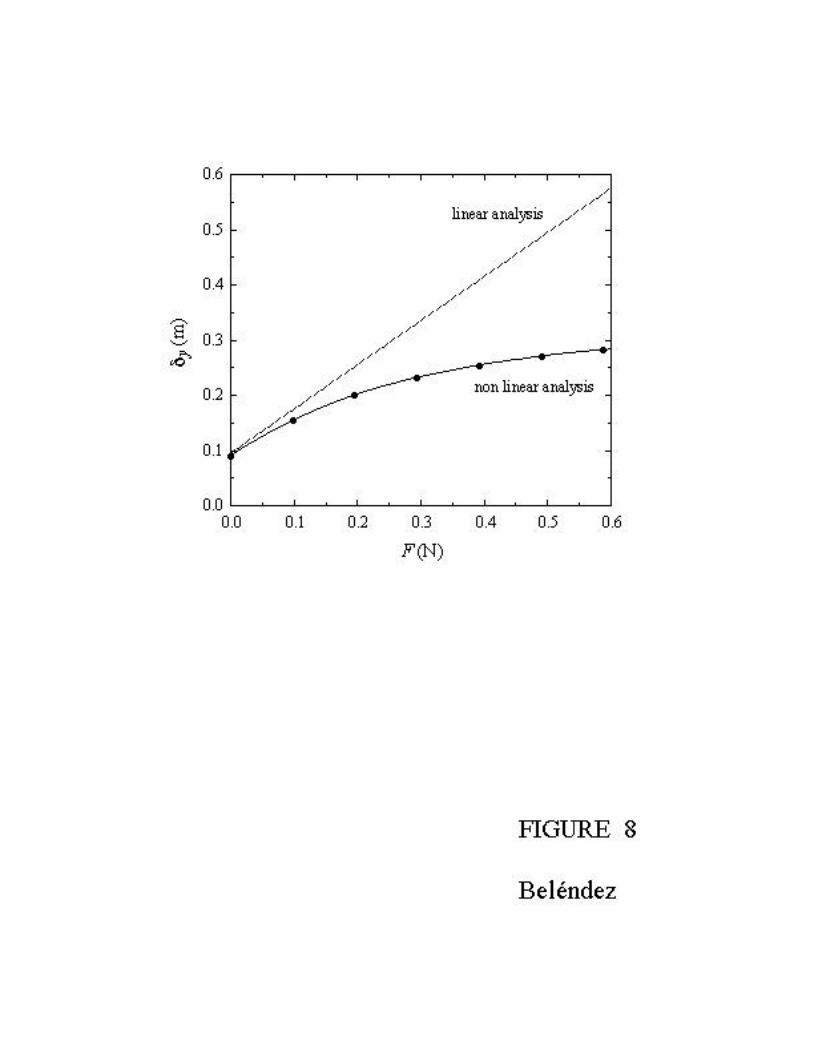
Figures 7 and 8 show the displacements at the free end of the cantilever beam,

δx and δy, as a function of the external vertical concentrated load F applied at the free

end. The dots correspond to the experimental data and the continuous lines to the

displacements numerically calculated with the help of the ANSYS program, using the

value obtained for Young’s modulus, E = 200 GPa. Comparing the experimentally

measured displacements with the calculated values, we can see that the agreement is

satisfactory.

In Figure 8 we have included the values of δy calculated, considering that the

behavior of the cantilever beam is linear (linear approximation for small deflections),

using the well-known equation for the vertical displacement at the free end for a

cantilever beam under the action of an external concentrated load F at the free end

and a uniformly distributed load W along its length [5, 11]:

)83(24

3

FWEI

Ly +=δ (15)

13

As we can see from Figure 6, the deflections calculated using equation (15) coincide

with the experimentally measured deflections only when the load F = 0, whereas for

all other applied loads the behavior of the beam is clearly nonlinear. As a part of the

study, students can then observe that the behavior of the cantilever beam analyzed in

this experiment may be considered linear when no external load is applied (F = 0), as

can be seen in Figure 8. If we consider F = 0 in equation (15), we obtain:

EI

WLy 8

3

=δ (16)

Applying the approximated equation (16) for the linear case and taking into account

that δy = 0.09 m for F = 0 (see Table I), we obtain E = 202 GPa for Young’s modulus,

which is practically the same value as that calculated using the ANSYS program.

Having calculated the value of E, we can verify that, using this value and with

the aid of the ANSYS program, it is possible to obtain the elastic curves for different

external loads, that is, the x and y coordinates of the horizontal and vertical deflection

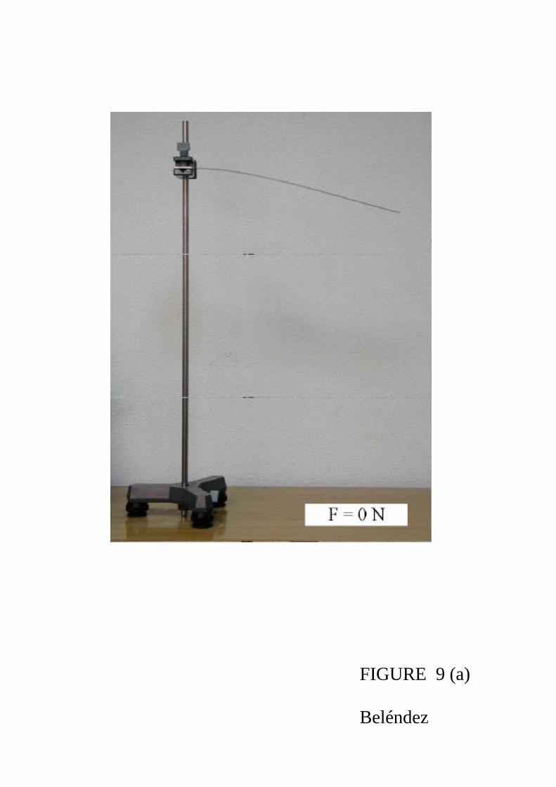
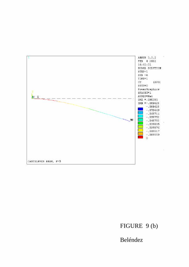
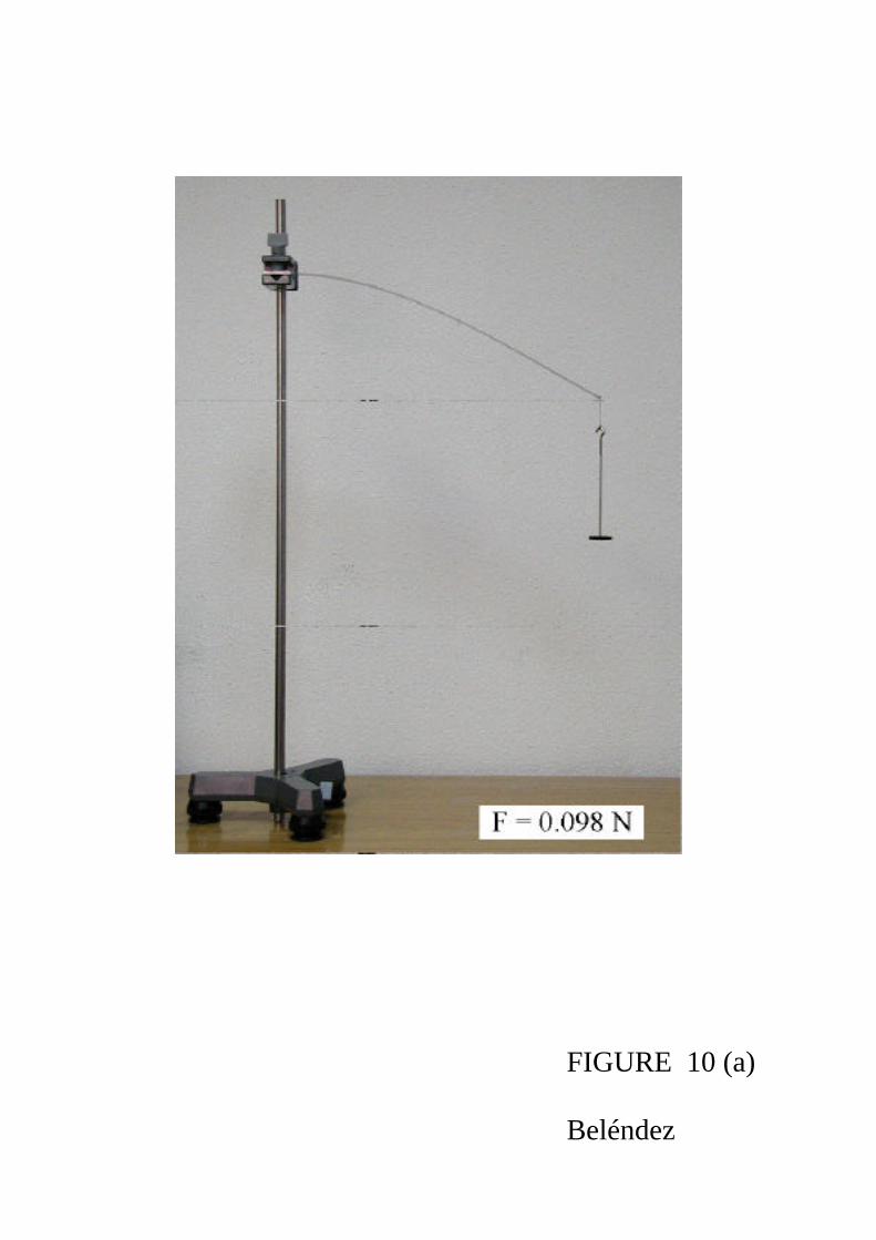
at any point along the neutral axis of the cantilever beam. Figures 9, 10 and 11 show

photographs of the experimental elastic curves as well as the simulations calculated

numerically with the aid of the ANSYS program, using E = 200 GPa, for F = 0, 0.098

and 0.196 N. Finally, in Figure 12, we have compared the experimentally measured

elastic curves with the numerically calculated ones, and we can see that the agreement

is satisfactory.

14

5.- CONCLUSIONS

We have studied the deflections of a cantilever beam theoretically, experimentally and

numerically. Firstly, we obtained the equations for large deflections, and by analyzing

this equation students can see that, although they are dealing with a simple physical

system, it is described by a differential equation with a non-linear term. On the other

hand, the experiment described in this paper provides students with not only an

understanding of geometric nonlinearity but also a better understanding of the basic

concepts of mechanics of materials. Important topics, including concentrated and

distributed loads, linear elastic materials, modulus of elasticity, large and small

deflections, moment-curvature equation, elastic curve, moments of inertia of the beam

cross-section or bending moment, are considered in this experiment.

The numerical study using the ANSYS program allows students not only to

solve the non-linear differential equation governing the nonlinear behavior of the

beam, but also to obtain the modulus of elasticity of the material and to compare the

experimentally and numerically calculated elastic curves of the beam for different

external loads. Finally, we have shown that the geometric nonlinear behavior of the

bending of a cantilever beam may be easily studied with a simple, easy-to-assemble,

low-cost experiment, which allows us to experimentally study the deflections of

cantilever beams by means of a series of simple measurements, such as lengths and

masses.

15

REFERENCES

[1] F. W. Riley and L. D. Sturges, Engineering Mechanics: Statis, Jonh Wiley &

Sons New York (1993)

[2] A. Bedford and W. Fowler, Engineering Mechanics: Statics, Addison Wesley,

Massachusetts (1996)

[3] D. J. McGill and W. W. King, Engineering Mechanics: Statics, PWS Publishing

Company, Boston (1995)

[4] S. P. Timoshenko, History of Strength of Materials, Dover Publications, New

York (1983)

[5] R. C. Hibbeler, Mechanics of Materials, Macmillan (1991)

[6] M. Sathyamoorthy, Nonlinear analysis of structures, CRC Press, Boca Raton FL

(1998).

[7] L. D. Landau and E. M. Lifshitz Course of Theoretical Physics, Vol. 7: Theory

of Elasticity, Pergamon Press, Oxford (1986)

[8] K. Lee, Large deflections of cantilever beams of non-linear elastic material

under a combined loading, Int. J. Non-linear Mech. 37, 439-43 (2002)

[9] ANSYS Documents, Swanson Analysis Systems, Inc., Houston PA, USA

[10] S. Moaveni, Numerical experiments for a Mechanics of Materials Course, Int. J.

Engng. Ed. 14, 122-129 (1998).

[11] A. Beléndez, C. Neipp and T. Beléndez, Experimental study of the bending of a

cantilever beam Rev. Esp. Fis. 15 (3) 42-5 (2001) in spanish

16

FIGURE CAPTIONS

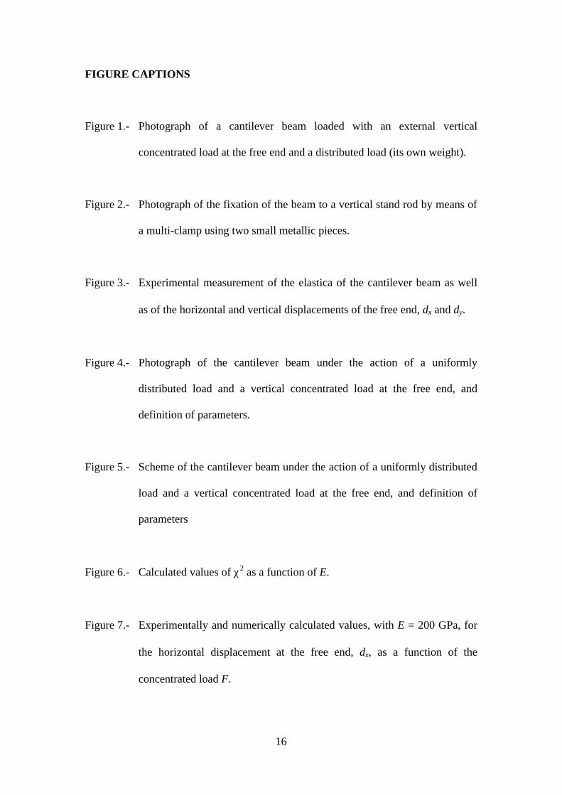
Figure 1.- Photograph of a cantilever beam loaded with an external vertical

concentrated load at the free end and a distributed load (its own weight).

Figure 2.- Photograph of the fixation of the beam to a vertical stand rod by means of

a multi-clamp using two small metallic pieces.

Figure 3.- Experimental measurement of the elastica of the cantilever beam as well

as of the horizontal and vertical displacements of the free end, δx and δy.

Figure 4.- Photograph of the cantilever beam under the action of a uniformly

distributed load and a vertical concentrated load at the free end, and

definition of parameters.

Figure 5.- Scheme of the cantilever beam under the action of a uniformly distributed

load and a vertical concentrated load at the free end, and definition of

parameters

Figure 6.- Calculated values of χ2 as a function of E.

Figure 7.- Experimentally and numerically calculated values, with E = 200 GPa, for

the horizontal displacement at the free end, δx, as a function of the

concentrated load F.

17

Figure 8.- Experimentally and numerically calculated values, with E = 200 GPa, for

the vertical displacement at the free end, δy, as a function of the

concentrated load F. The discontinuous line corresponds to the values

calculated using the approximative equation for small deflections (linear

analysis).

Figure 9.- Photograph of the experimental elastic curve together with the simulations

calculated numerically with the aid of ANSYS, using E = 200 GPa, for F

= 0 N.

Figure 10.- Photograph of the experimental elastic curve as well as the simulations

calculated numerically with the aid of ANSYS, using E = 200 GPa, for F

= 0.098 N.

Figure 11.- Photograph of the experimental elastic curve as well as the simulations

calculated numerically with the aid of ANSYS, using E = 200 GPa, for F

= 0.196 N.

Figure 12.- Experimentally measured and numerically calculated elastic curves for E

= 200 GPa.

TABLE I

F (N) δy (m) δy (m) Relative error

experimental (E = 200 GPa)

0 0.090 0.0896 0.45%0.098 0.154 0.1534 0.39%0.196 0.200 0.1995 0.25%0.294 0.231 0.2315 0.22%0.392 0.253 0.2540 0.39%0.490 0.270 0.2704 0.15%0.588 0.283 0.2827 0.11%

FIGURE 1

Beléndez

FIGURE 2

Beléndez

FIGURE 3

Beléndez

FIGURE 4

Beléndez

A(x,y)δy

L - δx

ϕ0

s

X

Y

F

δx

F w

w

FIGURE 5

Beléndez

FIGURE 7

Beléndez

F (N)

δ x(m

)

0.60.50.40.30.20.10.00.00

0.05

0.10

0.15

0.20

FIGURE 9 (a)

Beléndez

FIGURE 9 (b)

Beléndez

FIGURE 10 (a)

Beléndez

FIGURE 10 (b)

Beléndez

FIGURE 11 (a)

Beléndez

FIGURE 11 (b)

Beléndez

FIGURE 12

Beléndez

0.40.30.20.10.0

0.25

0.20

0.15

0.10

0.05

0.00

x (m)

y (m

)

F = 0 NF = 0.098 NF = 0.196 N

X

Y