NUMERICAL AND EXPERIMENTAL INVESTIGATION OF FLOW THROUGH A CAVITATING VENTURI

A THESIS SUBMITTED TO THE GRADUATE SCHOOL OF NATURAL AND APPLIED SCIENCES

OF MIDDLE EAST TECHNICAL UNIVERSITY

BY

BORA YAZICI

IN PARTIAL FULFILLMENT OF THE REQUIREMENTS FOR

THE DEGREE OF MASTER OF SCIENCE IN

AEROSPACE ENGINEERING

DECEMBER 2006

ii

Approval of the Graduate School of Natural and Applied Sciences

_____________________________

Prof. Dr. Canan ÖZGEN

Director

I certify that this thesis satisfies all the requirements as a thesis for the degree of

Master of Science.

____________________________

Prof. Dr. Đsmail Hakkı TUNCER

Head of Department

This is to certify that we have read this thesis and that in our opinion it is fully

adequate, in scope and quality, as a thesis for the degree of Master of Science.

_____________________________

Prof. Dr. Đsmail Hakkı TUNCER

Supervisor

Examining Committee Members

Prof. Dr. Sinan AKMANDOR (METU, AEE) ______________________

Prof. Dr. Đsmail Hakkı TUNCER (METU, AEE) ______________________

Prof. Dr. Yusuf ÖZYÖRÜK (METU, AEE) ______________________

Assoc. Prof. Dr. Abdullah ULAŞ (METU, ME) ______________________

Dr. Mehmet Ali AK (TÜBĐTAK, SAGE) ______________________

iii

I hereby declare that all information in this document has been obtained and

presented in accordance with academic rules and ethical conduct. I also

declare that, as required by these rules and conduct, I have fully cited and

referenced all material and results that are not original to this work.

Name, Last name:

Signature :

iv

ABSTRACT

NUMERICAL AND EXPERIMENTAL INVESTIGATION OF FLOW

THROUGH A CAVITATING VENTURI

Yazıcı, Bora

M.Sc., Department of Aerospace Engineering

Supervisor: Prof. Dr. Đsmail Hakkı TUNCER

August 2006, 122 pages

Cavitating venturies are one of the simplest devices to use on a flow line to control

the flow rate without using complex valve and measuring systems. It has no moving

parts and complex electronic systems. This simplicity increases the reliability of the

venturi and makes it a superior element for the military and critical industrial

applications. Although cavitating venturis have many advantages and many areas of

use, due to the complexity of the physics behind venturi flows, the characteristics of

the venturies are mostly investigated experimentally. In addition, due to their

military applications, resources on venturi flows are quite limited in the literature.

In this thesis, venturi flows are investigated numerically and experimentally. Two

dimensional, two-dimensional axisymmetric and three dimensional cavitating

venturi flows are computed using a commercial flow solver FLUENT. An

experimental study is then performed to assess the numerical solutions. The effect

of the inlet angle, outlet angle, ratio of throat length to inlet diameter and ratio of

throat diameter to inlet diameter on the discharge coefficient, and the oscillation

behavior of the cavitating bubble are investigated in details.

v

Keywords: Cavitation, Venturi, Multiphase Flow, Computational Fluid Dynamics,

Experimental

vi

ÖZ

KAVĐTASYONLU VENTURĐDEKĐ AKIŞIN SAYISAL VE DENEYSEL

ĐNCELENMESĐ

Yazıcı, Bora

Y. Lisans, Havacılık ve Uzay Mühendisliği Bölümü

Tez Yöneticisi: Prof. Dr. Đsmail Hakkı TUNCER

Ağustos 2006, 122 sayfa

Kavitasyonlu venturiler, komplex vana ve ölçüm sistemleri kullanılmadan akış

hatlarında debi kontrolü yapmak için kullanılabilecek en basit elemanlardandır.

Hiçbir karmaşık elektronik sistem ve hareketli parça ihtiva etmezler. Bu basitlik,

kavitasyonlu venturileri güvenilirliğini arttırarak askeri ve kritik endüstriyel

uygulamalarda üstünlük sağlamaktadır. Bu avantajlarına ve geniş uygulama

alanlarına rağmen, arkalarındaki kompleks fizikten dolayı, venturilerin

karakteristikleri genelde deneysel olarak yapılan çalışmalardan elde edilmiştir.

Askeri uygulamalarda sıkça kullanıldıklarından dolayı literatürde az sayıda belgeye

ulaşılabilmektedir.

Bu tez kapsamında, ticari akış çözücü olan FLUENT ile çeşitli kavitasyonlu venturi

geometrileri iki boyutlu, iki boyutlu eksenel simetrik ve üç boyutlu olarak

incelenmiştir. Akış çözümleyici programı doğrulamak için bir deneysel çalışma

yapılmıştır. Böylece giriş açısı, çıkış açısı, boğaz uzunluğunun giriş çapına oranı ve

boğaz çapının giriş çapına oranı gibi parametrelerin Çıkış sabiti ve salınım

davranışları üzerindeki etkisi incelenmiştir.

vii

Anahtar Kelimeler: Kavitasyon, Venturi, Çok Fazlı Akış, Hesaplamalı Akışkanlar

Mekaniği, Deneysel

viii

To My Parents

ix

ACKNOWLEDGMENTS

I would like to express my deepest thanks and gratitude to Prof. Dr. Đsmail Hakkı

TUNCER for his supervision, encouragement, understanding and constant

guidance.

Also I would like to express my gratitude to Dr. Mehmet Ali AK and Fatoş E.

ORHAN for initializing and supporting this thesis.

I would like to express my sincere appreciation to Mr. Erhan KAPLAN, Mr. M.

Cengizhan YILDIRIM and Mr. Bülent SÜMER for their crucial advices and

invaluable efforts during the preparation of this thesis.

My gratitude is endless for my family, without whom this thesis would not have

been possible.

x

TABLE OF CONTENTS

PLAGIARISM............................................................................................... iii

ABSTRACT................................................................................................... iv

ÖZ................................................................................................................... vi

ACKNOWLEDGMENTS............................................................................ ix

TABLE OF CONTENTS.............................................................................. x

LIST OF TABLES........................................................................................ xiii

LIST OF FIGURES...................................................................................... xiv

LIST OF SYMBOLS.................................................................................... xviii

CHAPTERS

1. INTRODUCTION.................................................................................... 1

1.1 Applications of Venturi...................................................................... 2

1.1.1 Flow Limiter.......................................................................... 2

1.1.2 Mixture Ratio Control............................................................ 3

1.1.3 Injector................................................................................... 4

1.1.4 Actuator Movement Equalizers............................................. 5

1.1.5 Fire of Disaster Control.......................................................... 6

1.2 Literature Survey................................................................................ 6

1.3 Research at TÜBĐTAK-SAGE........................................................... 7

1.4 Objective of the Thesis...................................................................... 14

2. VENTURI AND CAVITATING FLOWS............................................. 15

2.1 Cavitation........................................................................................... 15

2.2 Speed of Sound in Multiphase Flows & Choking Phenomenon........ 18

2.3 Dimensionless Parameters................................................................. 19

2.3.1 Cavitation Number................................................................. 19

2.3.2 Reynolds Number.................................................................. 20

2.3.3 Discharge Coefficient............................................................ 20

2.3.4 Strouhal Number.................................................................... 21

2.4 Preliminary Calculations with Bernoulli Equation............................ 22

xi

3. NUMERICAL METHOD....................................................................... 24

3.1 Numerical Methodology.................................................................... 24

3.2 FLUENT Theory................................................................................ 25

3.3 FLUENT Cavitation Model............................................................... 26

3.3.1 Continuity Equation for the Mixture...................................... 27

3.3.2 Momentum Equation for the Mixture.................................... 28

3.3.3 Energy Equation for the Mixture........................................... 29

3.3.4 Volume Fraction Equation for the Secondary Phases............ 29

3.3.5 FLUENT Cavitation Model Validation Case- Cavitation

Over A Sharp Edged Orifice............................................................ 30

4. EXPERIMENTAL STUDY.................................................................... 35

4.1 Experimental Setup............................................................................ 35

4.1.1 Test Section............................................................................ 36

4.2 Measurements.................................................................................... 39

4.2.1 Pressure Measurements......................................................... 39

4.2.2 Mass Flow Rate Measurements............................................. 39

4.2.3 Visual Observations.............................................................. 39

5. RESULTS & DISCUSSIONS................................................................ 40

5.1 Numerical Solutions........................................................................... 40

5.1.1 Numerical Solution Matrix.................................................... 40

5.1.2 2-D Axisymmetric Solutions................................................. 47

5.1.3 2-D Solutions......................................................................... 52

5.1.4 Effect of the Wall Depth......................................................... 74

5.1.5 Summary of Numerical Simulations...................................... 77

5.2 Experimental Results......................................................................... 78

5.2.1 Experiment Matrix................................................................. 78

5.2.2 Experiments with Axisymmetric Venturi Flows................... 79

5.2.3 Previous Engine Tests in TÜBĐTAK-SAGE......................... 97

5.2.4 Failure in the Experiments with 3-D Prismatic Venturies..... 98

6. CONCLUSION......................................................................................... 99

REFERENCES.............................................................................................. 101

xii

APPENDIX A: EXPERIMENTAL SETUP TECHNICAL

DRAWINGS & MEASURMENT EQUIPMENT...................................... 103

APPENDIX B: RESULTS OF NUMERICALS SIMULATIONS.......... 112

xiii

LIST OF TABLES

Table 3-1. Mesh Size Versus Cavitation Number for FLUENT Validation

Case at 50 bar.................................................................................................. 34

Table 4-1. Geometric Properties of the Axisymmetric Venturies................... 37

Table 5-1. Solution Matrix for Numerical Solutions...................................... 42

Table 5-2. Oscillation Frequency for 2-D, 2-D Axisymmetric and 3-D

Prizmatic Solutions......................................................................................... 76

Table B-1. Vapor Pressure vs. Temperature................................................... 112

Table B-2. Geometric Properties of the Venturies for 3-D Prismatic Test

Section............................................................................................................. 116

Table B-3. Results of 2-D Axisymmetric Numerical Simulations................. 117

Table B-4. Results of 2-D Numerical Simulations at Re=6E5....................... 121

xiv

LIST OF FIGURES

Figure 1-1. Sample Drawing of a Cavitating Venturi................................... 1

Figure 1-2. Simple Use of Cavitating Venturies with Pumps [1]................. 3

Figure 1-3. Mixture Ratios can be Controlled by Using Two Venturies for

Each of the Fuel and Oxidizer Lines [1]....................................................... 4

Figure 1-4. Cavitating Venturi was Used to Mix the Detergent and Water

at a Constant Ratio [1]................................................................................... 4

Figure 1-5. Cavitating Venturies can be Used to Equalize the Actuator

Movement, a), or to Equalize the Displacement System of a Trust Vector

Control System [1]. ...................................................................................... 5

Figure 1-6. A Typical Illustration for Fire or Disaster Control Application

[1].................................................................................................................. 6

Figure 1-7. Sketch of Test Setup Developed in TÜBĐTAK-SAGE.............. 8

Figure 1-8. Data Obtained from the Pressure Transducers........................... 9

Figure 1-9. Technical Drawing of the Tested Venturi, All Dimensions in

mm................................................................................................................. 10

Figure 1-10. Comparison of the Result Obtained from 1-D Solutions,

FLUENT and the Experiments...................................................................... 10

Figure 1-11. Pressure Measurement which Took from Outlet of the

Designed Venturi from a Liquid Propellant Rocket Engine Test................. 11

Figure 1-12. Pressure Data Acquired from the cavitating Venturi Test........ 12

Figure 1-13. Volume Fraction of Liquid Water............................................ 13

Figure 1-14. Pressure Through Venturi......................................................... 13

Figure 2-1. Pressure Distribution Through Venturi...................................... 16

Figure 2-2. Volume Fraction of Liquid Phase Through Venturi................... 17

Figure 2-3. Velocity Field Through Venturi................................................. 17

Figure 2-4. Sonic Velocity of Water/Bubble Mixture w.r.t.

Air Volume Fraction..................................................................................... 18

Figure 3-1. FLUENT Validation Case Geometry......................................... 31

xv

Figure 3-2. FLUENT Validation Case Results............................................. 32

Figure 3-3. Results for the FLUENT Validation Case at 50 bar Inlet

Pressure......................................................................................................... 33

Figure 4-1. Test Setup Sketch....................................................................... 36

Figure 4-2. Picture of Tested Venturies........................................................ 38

Figure 4-3. Picture of High Speed Camera................................................... 39

Figure 5-1. Geometric Parameters are Given on a Generic Venturi............. 42

Figure 5-2. Pressure (Pa) Field Through a Generic Venturi......................... 43

Figure 5-3. Velocity (m/s) Field Through a Generic Venturi....................... 44

Figure 5-4 Liquid Phase Volume Fraction for a Generic Venturi................. 45

Figure 5-5. Liquid Phase Volume Fraction for a Generic Venturi Throat.... 45

Figure 5-6. Mach Contour Plot for a Generic Venturi.................................. 46

Figure 5-7. Flow Path Lines Colored with Phase Volume Fractions for

Case σ2........................................................................................................... 49

Figure 5-8. Variation of the Volume Fraction of Vapor Phase for Sample

Venturi Geometry at σ2................................................................................. 52

Figure 5-9. Unsteady Oscillation at the Exit Plane of the Venturi................ 53

Figure 5-10. The Effect of Oscillating Cavitation Bubble on the Inlet

Mass Flow Rate............................................................................................. 53

Figure 5-11. Discharge-Coefficient (Cd) vs. Ф1 for 2D –Axisymmetric

Solutions at Re=6E5 for Dth/Din=0.357......................................................... 58

Figure 5-12. Discharge-Coefficient (Cd) vs. Ф1 for 2D –Axisymmetric

Solutions at Re=6E5 for Dth/Din =0.714........................................................ 59

Figure 5-13. Discharge-Coefficient (Cd) vs. Ф2 for 2D –Axisymmetric

Solutions at Re= 6E5 for Dth/Din=0.357........................................................ 60

Figure 5-14. Discharge-Coefficient (Cd) vs. Ф2 for 2D –Axisymmetric

Solutions at Re= 6E5 for Dth/Din=0.714........................................................ 61

Figure 5-15. Discharge-Coefficient (Cd) vs. Ф1 for 2D Solutions at

Re=6E5 for Dth/Din=0.357............................................................................. 62

Figure 5-16. Discharge-Coefficient (Cd) vs. Ф1 for 2D Solutions at

Re=6E5 for Dth/Din=0.714............................................................................. 63

xvi

Figure 5-17. Discharge-Coefficient (Cd) vs. Ф2 for 2D Solutions at

Re=6E5 for Dth/Din=0.357............................................................................. 64

Figure 5-18. Discharge-Coefficient (Cd) vs. Ф2 for 2D Solutions at

Re=6E5 for Dth/Din=0.714............................................................................. 65

Figure 5-19. Effect Lth/Din on Discharge-Coefficient (Cd) vs. Ф2 for 2D-

Axisymmetric Solutions at σ1........................................................................ 66

Figure 5-20. Effect Dth/Din on Discharge-Coefficient (Cd) vs. Ф2 for 2D-

Axisymmetric Solutions at σ1........................................................................ 67

Figure 5-21. Effect Lth/Din on Discharge-Coefficient (Cd) vs. Ф2 for 2D

Solutions at σ1............................................................................................... 68

Figure 5-22. Effect Dth/Din on Discharge-Coefficient (Cd) vs. Ф2 for 2D

Solutions at σ1............................................................................................... 69

Figure 5-23. 2D- Axisymmetric Solutions vs. 2D Solutions for

Dth/Din=0.357 at σ1........................................................................................ 70

Figure 5-24. 2D- Axisymmetric Solutions vs. 2D Solutions for Dth/Din=0.

0.714 at σ1 ..................................................................................................... 71

Figure 5-25. Reynolds Number Effect on Discharge Coefficient on

Axisymmetric Venturi Flows for Dth/Din=0.357 at σ1................................... 72

Figure 5-26. Reynolds Number Effect on Discharge Coefficient on

Axisymmetric Venturi Flows for Dth/Din=0. 0.714 at σ1 .............................. 73

Figure 5-27. Effect of wall for 3-D Prismatic Solutions at σ1....................... 75

Figure 5-28, Discharge Coefficient vs. 2-D, 2-D Axisymmetric and 3-D

Prismatic Solutions........................................................................................ 76

Figure 5-29. High Speed Camera Plot.......................................................... 80

Figure 5-30. a) Pressure vs. Time b) Cavitation Number vs. Time.............. 80

Figure 5-31. High Speed Camera Plots........................................................ 82

Figure 5-32. a) Pressure vs. Time b) PSD vs. Frequency (Hz)

c) Cavitation Number vs. Time..................................................................... 83

Figure 5-33. a) Pressure vs. Time b) Cavitation Number vs. Time c) PSD

vs. Frequency (Hz) d) Waterfall Diagram of Exit Pressure.......................... 85

Figure 5-34. High Speed Camera Plots........................................................ 86

xvii

Figure 5-35. a) Pressure vs. Time b) Cavitation Number vs. Time c) PSD

vs. Frequency................................................................................................ 88

Figure 5-36. High Speed Camera Plots........................................................ 89

Figure 5-37. Pressure vs. Time b) Cavitation Number vs. Time c) PSD vs.

Frequency...................................................................................................... 90

Figure 5-38. High Speed Camera Plot.......................................................... 91

Figure 5-39. a) Pressure vs. Time b) Cavitation Number vs. Time c) PSD

vs. Frequency................................................................................................ 92

Figure 5-40. High Speed Camera Plots........................................................ 93

Figure 5-41. a) Pressure vs. Time b) Cavitation Number vs. Time c) PSD

vs. Frequency................................................................................................ 94

Figure 5-42. High Speed Camera Plots......................................................... 95

Figure 5-43. a) Pressure vs. Time b) Cavitation Number vs. Time c) High

Speed Camera Plot........................................................................................ 96

Figure 5-44. Engine Combustion Chamber Pressure Data........................... 97

Figure 5-45. Engine Combustion Data Frequency Analysis......................... 98

Figure A2-1. Data Acquisition System......................................................... 109

Figure A2-2. Pressure Transducer................................................................. 110

Figure A2-3. Hoffler Turbine Type Flow Meter........................................... 110

Figure A2-4. Pressure Regulator................................................................... 111

Figure B-1. Vapor Pressure of Water vs. Temperature................................. 113

Figure B-2. Strouhal Number vs. Outlet Angle............................................ 113

Figure B-3. CAD Drawing of The Test Section and the Adaptors............... 114

Figure B-4.Parts of the 3-D Prismatic Test Section...................................... 114

Figure B-5. Assembly of the 3-D Prismatic Test Section............................. 115

Figure B-6.Four Different Venturi Configuration for 3-D Prismatic Test

Section........................................................................................................... 115

xviii

LIST OF SYMBOLS

Cc Core coefficient

Cd Discharge coefficient

Pv Vapor pressure

σ Cavitation number

Vth Throat velocity

ρl Liquid density

ρm Density of Mixture

µl Liquid viscosity

µm Viscosity of Mixture

Din Inlet Diameter

Dth Throat Diameter

Re Reynolds number

•

m Mass flow rate

idealm•

Ideal Mass flow rate

realm•

Real Mass flow rate

St Strouhal number

f Frequency of oscillation

LD Length of the diffuser part of venturi

Lth Throat length

Ac Core area

Ф1 Inlet angle (deg)

Ф2 Outlet angle (deg)

αk Volume fraction of phase k

Hd Hydraulic diameter

Tu Turbulence intensity

1

CHAPTER 1

INTRODUCTION

Cavitating venturis are one of the simplest flow control devices and are widely

used in a range of industries. Numerous industrial flow processes are controlled by

such devices. They are commonly used to meter propellants in liquid rocket engine

tests by controlling the mixture ratio of the fuel and the oxidizer. The fact that

venturies may provide a constant flow rate under varying downstream pressure,

they are particularly useful during the ignition transient when the downstream

pressure in the combustion chamber rises rapidly.

A cavitating venturi typically consists of a converging section, a short straight

throat section, and a diffuser as shown in Figure 1-1. When the downstream

pressure P2 is less than 85-90% of upstream pressure P1, the flow may cavitate at

the throat, and flow through the venturi orifice becomes “choked”. In general, a

further decrease in the downstream pressure does not influence the mass flow rate.

Figure 1-1.Sample Drawing of a Cavitating Venturi, Cavitating Part is Illustrated as

Black.

In spite of wide use of venturies, relatively little research data on its operating

characteristics and on the mechanisms of operation are available in literature.

2

Moreover, there is almost no data in literature about the influence the geometric

parameters on the performance of the cavitating venturies.

In this chapter, the general applications of the cavitating venturies are discussed in

detail, and a literature survey on cavitating venturi flows is given. In addition, the

previous studies on venturi flows conducted at TÜBĐTAK-SAGE are summarized

1.1 Applications of Venturi

Cavitating venturies can be used in applications where a passive liquid flow control

system is required. Venturies are widely utilized in

•••• Flow Limiters

•••• Mixture Ratio Controllers

•••• Injectors

•••• Actuator Movement Equalizers

•••• Fire Extinguishers

1.1.1 Flow Limiter

A cavitating venturi can be used in two modes; one is the “cavitating” mode and

the other is “non-cavitating” mode. If the pressure drop is not sufficient enough to

cause the cavitation at the throat of the venturi, the second mode prevails. A venturi

in a flow system switching between these two modes can be used as a flow limiter.

If the back pressure decreases suddenly, flow will be choked so that the flow rate

will be limited to a certain value. In the “non-cavitating” mode, the venturi can also

be used as a flow measurement device.

A primary application for this kind of usage is seen in combustion systems. At the

start up of the combustion process, when the back pressure is low, the fuel flow

rate may be limited with a cavitating venturi. As the transient back pressure in the

3

combustion chamber rises, the cavitation stops and the venturi switches to its

second mode.

Flow limiting feature of cavitating venturi can also be used to limit the flow rate of

a centrifugal pump system. In Figure 1-2, Head (H) vs. Flow rate (Q) curves of

pump and venturi plotted on the same graph. The intersection point will be the

maximum flow point and further increase in available energy will not increase the

flow rate after this maximum value is reached.

Figure 1-2. Simple Use of Cavitating Venturies with Pumps [1].

1.1.2 Mixture Ratio Controllers

Cavitating venturies will control the mixture ratio of any type of fluids and gasses.

One of the best examples is the rocket engine’s oxidizer to fuel ratio control

application. As it is illustrated in Figure 1-3, where two fluids are fed through the

combustion chamber from different lines. As long as the chamber pressure is below

the pressure recovery limits of the venturies, the mixture ratio and flow rates may

be kept constant. It should be noted that if venturies are not used, the flow in the

feeding lines respond to the chamber pressure, and it will be impossible to keep the

mixture ratios fixed.

4

In gas – fluid mixture cases venturies can similarly be used together with a sonic

choke nozzle to control the mixture ratio.

Figure 1-3. Mixture Ratios can be Controlled by Using Two Venturies for Each of

the Fuel and Oxidizer Lines [1].

1.1.3 Injector

Through the throat of the cavitating venturi pressure will fall to the vapor pressure

of the working fluid. Therefore, creation of such vacuum condition at the throat

will be used to suck another fluid to mix with the working fluid. In Figure 1-4, a

simple example is given for the mixture of detergent and water.

Figure 1-4. Cavitating Venturi was Used to Mix the Detergent and Water at a

Constant Ratio [1].

5

1.1.4 Actuator Movement Equalizers

Cavitating venturies can be used in hydraulic motors and multiple actuators to

provide uniform displacement. The displacement of actuators under varying loads

can be equalized as long as the inlet pressure of the venturies is kept constant.

a)

b)

Figure 1-5. Cavitating Venturies can be Used to Equalize the Actuator Movement,

a), or to Equalize the Displacement System of a Trust Vector Control System [1].

An example for the actuator applications is the control of the displacement of a

platform under non-uniform loading, which is given in Figure 1-5a. The cavitating

venturi may provide a constant flow rate into the actuators, thus a uniform motion

for the platform, independently from the loading on each actuator.

6

In Figure 1-5b the equalization of the actuators of a thrust vector control system is

illustrated. With the use of a cavitating venturi, regardless of the loads acting on the

nozzle plates, their displacements are equalized.

1.1.5 Fire or Disaster Control

For an extinguishing system one of the most critical problems is the difficulty of

equalizing the flow rate between the branches of spray nozzles. Moreover, if one or

several of them fail or damaged, a huge amount of extinguishing fluid will be

directed to these lines rather than the other spray nozzles. So the whole system may

fail in a short time. With the use of a cavitating venturi although some of the lines

are damaged or burn-out, the flow rate through the other lines will not be affected.

In Figure 1-6, a simple schematic view is illustrated.

Figure 1-6. A Typical Illustration for Fire or Disaster Control Application. [1]

1.2 Literature Survey

Although cavitating venturies are widely used, publications on venturi flows are

quite limited on literature. Early studies carried out by Fox Z. [1] are about the

usage of a cavitating venturi to overcome the startup transient in rocket

applications. Fox investigates the basic application of a venturi and its sizing

features. Through seventies, the theoretical bases of cavitating flows are

investigated by Boure, Fritte [2] and K.H. Ardron [3]. However the experimental

studies on the effect of geometric properties of cavitating venturies are limited.

7

Several experiments are conducted by K.H. Ardron and D.W. Harvey at the NASA

Lewis Research Center on the usage of cryogens in cavitating venturies [4]. These

tests lead to the foundation of theoretical and numerical techniques to predict the

behavior of flow through cavitating venturies. N.T. Thang and M.R.Davis in their

theoretical work present the pressure distribution of a bubbly flow through the

cavitating venturies and discuss the shockwaves created in cavitating venturies [5].

They later validate their theoretical findings through some experiments. But the

main difference of this study is that the fluid is assumed to be a homogenous

bubbly mixture of air and liquid water. This assumption allows them to simplify

the equations governing the cavitating venturi flows.

At the beginning phases of Computational Fluid Dynamics, M. J. Gaston and J.A.

Reizes tries to model bubble dynamics though a venturi with a potential flow

solver[6]. Two years later J.D. Sherwood proposes a potential flow solution of a

deforming bubble in a venturi [7]. Nevertheless, none of them is able to model the

inception phases of cavitation and the collapse phase of the bubbles through a

heterogeneous media.

Recently with the increasing power of the computers and the rising of commercial

flow solvers through the this area several numerical simulations were performed

with in-house and commercial flow solvers by G. P. Salvador and S. H. Grankel[8].

And one of the best works is proposed by Changhai Xu & Stephan D. Heister [9].

They describe the state of art of cavitating venturi flows with experimental studies

and numerical calculations, and they point out the importance of the oscillatory

features at the diffuser part of the venturi. They also comment on the effects of the

Reynolds number on the oscillation behavior.

1.3 Research at TÜBĐTAK – SAGE

In a research project carried out by TÜBĐTAK–SAGE in 2003, Turkey’s first

operational liquid propellant rocket engine was designed, manufactured and tested.

In this study the flow rate of the oxidizer and the fuel was mainly controlled by two

8

cavitating venturies. At the beginning phase of the project, due to the time and the

financial limitations, instead of using an active flow control system, cavitating

venturies were employed as a passive flow control system. Due to export license

restriction on venturies in regard to military applications on rocket engines,

purchasing of venturies from abroad wasn’t successful. Therefore, a research

project has started on developing and testing cavitating venturies. The performance

of the cavitating venturies were calculated easily with the 1-D Bernoulli equations

which is presented later in this thesis in detail [10], [11]. However, this simplified

method can not predict the flow rate accurately. Since, these simplified equations

do not account for the effect of the geometric properties like, the inlet angle, outlet

angle and the throat length or inlet to throat diameter ratios.

To investigate the performance of the cavitating venturies, a simple test setup was

designed and assembled. Several tests were conducted with several venturies but

because of the restrictions on time of the on going project, the number of different

venturies and the number of tests were limited. The working fluid in these tests was

water due to the difficulty of using reactive oxidizers and fuels in the tests. In

addition, a commercial flow solver FLUENT was also to predict the cavitating

flows and the characteristics of the cavitating venturies.

Figure 1-7. Sketch of Test Setup Developed in TÜBĐTAK-SAGE

9

A simplified sketch of the test setup is given as figure 1-7. A high pressure

gaseous nitrogen tank is used to pressurize the water tank and three pressure

transducers are used to measure the tank pressure, inlet pressure and outlet pressure

of the venturi. At this test setup, venturi exit is open to the atmosphere so the tests

are performed with a constant cavitation number. The average flow rate through the

venturi is measured through the remaining water in the tank.

Figure 1-8. Data Obtained from the Pressure Transducers.

The dimensional data for the venturi are given in Figure 1-9. In Figure 1-8,

pressure measurements taken from a typical venturi flow is given. Initially the

pressure at the venturi inlet, outlet and in the tank are all the same. When the valve

opened, the outlet pressure drops to vapor pressure and flow is choked in a few

milliseconds. This measurement shows how a cavitating venturi responds quickly

and restricts the flow rate.

10

Figure 1-9. Technical Drawing of the Tested Venturi, All Dimensions in mm.

Figure 1-10. Comparison of the Result Obtained from 1-D Solutions, FLUENT and

the Experiments.

In Figure 1-10, the mass flow rates which are calculated with 1-D flow solutions,

FLUENT, and measured in the experimental study tests are given. In Figure 10,

one can see the 1-D calculations made for two different Cc values. Where Cc is the

effective liquid throat area ratio or “Core Coefficient”, which can not be calculated

with 1-D equations and is a constant value for every different geometries.

Experiments were performed for four different inlet pressures while keeping the

exit pressure equal to ambient pressure. Except the one in the 100 bars, FLUENT

predictions compare well with the experimental data. 1-D solution with the Cc

value equal to one predicts a mass flow rate 20% higher at very high pressures. In

case of a rocket engine firing, this excess fuel or oxidizer may cause a failure or a

performance loss which is not acceptable.

11

Figure 1-11. Pressure Measurement which Taken from Outlet of the Designed

Venturi from a Liquid Propellant Rocket Engine Test

The time variation of pressure data acquired from an engine firing test is given in

Figure 1-11 to describe how a cavitating venturi works in a real engine test

environment. One of the pressure transducers is placed to the exit of the venturi and

the other one is placed in the combustion chamber. At the beginning of the ignition,

the venturi exit pressure is equal to the tank pressure. After the main fuel and the

oxidizer valves are opened, the venturi exit pressure decreases to vapor pressure.

Following the ignition process, the pressure wave goes through the feed lines, and

the exit pressure of the venturi is seen to be kept almost constant at about a certain

value.

12

Figure 1-12. Pressure Data Acquired from the Cavitating Venturi Test. Blue line

represents the inlet pressure and the Green line represents the exit pressure of the

cavitating venturi.

The uncertainty of the effect of geometry on the performance of the cavitating

venturi will cause delays on the time schedule of a project. In Figure 1-12, pressure

measurements taken at the inlet and the exit of a cavitating venturi, which has the

same inlet and outlet angles except the throat diameter increased two times than the

venturi which the dimensions is given in Figure 1-9, is plotted. At this Figure,

although the exit pressure was the ambient pressure, the exit pressure oscillates at

30 bar level, which is very different from the previous result given at Figure 1-8.

Mass flow rate measurement also shows that the venturi is not choked properly.

After further analyses performed with FLUENT, the venturi seems to be choked

well due to the results which are given in Figure 1-13 and Figure 1-14. Therefore,

doubts about the solver and the capabilities rise at this moment. And it is necessary

to understand the limits of the solver for not to face with same problems in the

13

future. Also in future projects the design iterations have to be minimized to reduce

the production and testing costs.

Figure 1-13. Volume Fraction of Liquid Water, red represents the fully liquid water

zone and the blue represent the fully liquid vapor zone.

Figure 1-14. Pressure Through Venturi

14

Objective The Thesis

The aim of this thesis is to investigate the effect of geometry on the behavior of the

cavitating venturi flows. This work mainly focuses on the effect of inlet, outlet

angles and the dimensionless throat length on similar flows. The similarity

parameters are chosen to be cavitation number which will be defined further and

the Reynolds number, which has a characteristic length of the throat diameter. In

addition, through the tests and numerical solution, the working fluid is water.

The effect of the geometry on the cavitating venturi flows is investigated with the

commercial flow solver. But it is necessary to validate the solutions and tune the

parameters of the solver. Although FLUENT has a validation case for cavitation

through an orifice, due to the past experience, which is described in previous

chapters, an experiment setup is designed and manufactured through this thesis.

Validation case is also used to experiment on the mesh size dependency of the

cavitating flows. And for a better visual observation, although all cavitating

venturies are axis-symmetric, the test setup is designed to be 3-D Prismatic

geometry. After obtaining the results of the 2-D axisymmetric cases, the cases

which have interesting phenomenons like oscillations etc. These results are

compared with the similar 2-D results and then will be tested experimentally to

tune the flow solver. This methodology is seemed to be cumbersome but in order to

obtain meaningful results it is necessary to do so.

In first two chapters, basics of cavitating flows and the areas of use of cavitating

venturies are discussed in order to give background knowledge about the

dimensionless parameters and the flow characteristics of venturi flows. The

numerical methodology and Experimental setup are discussed in the third and the

forth chapters. Also the experimental values that have to be measured and the

experimental setup are discussed in the fourth chapter. In the fifth chapter the

results of numerical solutions and the experiments were used to develop some

engineering graphs. Also in this chapter the numerical and experimental matrixes

are stated in details.

15

CHAPTER 2

VENTURI AND CAVITATING FLOWS

To understand cavitating venturi flows, it is better to give background information

about the cavitation process. Also to understand the chocking phenomenon one has

to investigate the speed of sound in multiphase flows and how the second phase

affects the characteristics of the flow field. Moreover, to obtain more meaningful

results it is necessary to define the geometry and the flow parameters with the non-

dimensional numbers like Reynolds number which governs the viscosity effects

and cavitation number which is a value to judge the strength of cavitation. Through

this chapter also the basic calculation methods which depends on zero dimensional

flow assumptions is also investigated in details.

2.1 Cavitation

A liquid at constant temperature could be subjected to decreasing pressure, P,

which falls below the saturated vapor pressure, Pv. The value of (Pv-P) is called the

tension, ∆P, and the magnitude at which rupture occurs is the tensile strength of the

liquid, ∆Pc. The process of rupturing a liquid by decreasing in pressure at roughly

constant liquid temperature is often called cavitation. If a liquid at constant

pressure subjected to an increasing temperature above its critical temperature again

the liquid will rupture by the increase in tension but in this time it is called

‘boiling’. ‘Cavitation’ and ‘boiling’ are the names given to the way of rupturing of

the liquid in constant temperature or constant pressure respectively. [13]

At the inlet of the cavitating venturi throat, the flow is accelerated such that the

local static pressure decreases under the vapor pressure of the liquid. And the

cavitation bubbles created at the wall of the throat separates from the leading edge

16

of the throat section. These bubbles move through the diffuser part of the cavitating

venturi and collapse into smaller bubbles and disappear at a specific length due to

the pressure recovery at the diffuser part. To the time that the bubbles created to the

disappeared through the venturi at the locations where the bubbles exists the local

pressure is set to the vapor pressure at that section of the venturi. In Figure 2-1, 2-2

and 2-3 the pressure distribution, the volume fraction of water and velocity

distribution through a venturi can be seen.

Figure 2-1. Pressure Distribution Through Venturi

17

Figure 2-2. Volume Fraction of Liquid Phase Through Venturi

Figure 2-3. Velocity Field Through Venturi

18

2.2 Speed of Sound In Multiphase Flows And Choking Phenomenon

In sonic choked gas nozzles which are counterpart of cavitating venturies in gas

flow, the flow at the throat is designed to attain Mach equal to `one` for the gas

involved. For homogenous gases, the calculation of the speed of sound is not

troublesome. In the case of liquid flow, choking phenomenon rather difficult to

predict due to the fact that the difficulty of calculating speed of sound at the

heterogeneous multiphase flow. In Figure 2-4, speed of sound is given as a function

of void fraction of gas in water for two different k values 1.0 and 1.4. [13]

Figure 2-4. Sonic Velocity of Water / Bubble Mixture w.r.t. Air Volume

Fraction.[13]

One have to keep in mind that Figure 2-4 is for homogenous bubble/liquid mixtures

and not applicable for heterogeneous flows. In cavitating venturies the flow field is

rather complex that to calculate the sonic velocity. Actually at the throat section

there exist layers of several mixture ratios. Near the wall the cavitation starts so

that the volume fraction ratio is close to 1. And a core of liquid remains at the

19

middle portion of the throat section of the venturi. Therefore, it is very difficult to

judge the ‘choking’ condition on such heterogeneous media.

2.3 Dimensionless Parameters

Cavitating venturi flows are affected from several geometric parameters, flow

parameters and liquid properties. Therefore, it is necessary to define dimensionless

similarity parameters so as to decrease number of solutions and experiments. In

cavitating venturi flows mainly there are two numbers which are important; one is

Reynolds Number and the second one is the cavitation number, which was defined

in detail below. Also there are two parameters which are used to analyze the flow

or compare the performances of the venturies. One is the discharge coefficient, Cd,

which defines the performance and the other is the Strouhal Number, St, which

defines the unsteady bubble oscillations behaviors.

2.3.1 Cavitation number

The cavitation number σ is the most important parameter in the present work as it

will set the overall extent of cavitation in the venturi. The cavitation number is

defined in equation 2-1 as follows [9].

21

1

PP

PP v

−

−=σ (2-1)

Where the P1 and P2 are inlet and outlet pressure, respectively and Pv is the vapor

pressure of the working fluid. If inlet pressure P1 is relatively bigger compared to

P2 the cavitation number have a value higher than 1. And in the limit cavitation

number has the value of 1 for the vacuum at the exit. Cavitation number is a

measure to compare the strength of the cavitation when the value decreases to 1 the

cavitation effect is strongest. After a certain value of the cavitation number

20

exceeded, cavitation process stops and the venturi lets the liquid flow with the mass

flow rate affected from the exit pressure P2.

2.3.2 Reynolds Number

The Reynolds Number “Re” measures viscous effects as in all Navies-Stokes

solutions. We choose the Bernoulli velocity as the throat Vth, the venturi throat

diameter Dth, liquid density ρl, and the dynamic viscosity µl as the dimensions of

Reynolds number as in literature, [9].

l

ththl DV

µρ

=Re (2-2)

With the increasing Reynolds number it is known that the oscillation exists in the

flow field damps out [9].To increase the Reynolds number without changing the

other parameters one has to increase the inlet pressure P1 and also increase exit

pressure such that the cavitation number stays constant.

2.3.3 Discharge Coefficient

For cavitating venturi flows discharge coefficient,” Cd”, can be defined in several

ways but through this thesis the definition will be the ratio of the real mass flow

rate to the ideal mass flow rate which is calculated with the Bernoulli velocity, Vth,

at the throat. Through out numerical solution and the experiments the real mass

flow rate is a known value and the ideal mass flow rate is calculated through the

following equations. Ideal mass flow rate calculation assumes all the throat area is

liquid and the core coefficient “Cc” is equal to one. To calculate the Vth one has to

use the equation 2-8 for a known vapor pressure and inlet pressure value.

21

ththlideal VAm ρ=•

(2-3)

ththlcreal VACm ρ=•

(2-4)

c

ththl

ththlc

ideal

real

d CVA

VAC

m

mC ===

•

•

ρρ

(2-5)

2.3.4 Strouhal Number

The oscillation of bubbles in the flow field is mainly due to the unsteady growth

and collapse of the bubbles which are generated at the throat inlet of the cavitating

venturi. In some applications like rocket engine flow control, these oscillations in

the flow field gain importance. These unsteady flow fluctuations may couple with

the combustion and induce instability on the flow field or can affect the

performance of the injector atomizers. Although FLUENT does not govern the

bubble formation and collapse, these effects can be seen on some high cavitation

number values also which FLUENT can calculate. Here in equation 2-6, f, is the

frequency of oscillations in Hz and Vth is the throat liquid velocity which is

calculated with Bernoulli equation, and the LD is the length of the diffuser part of

the venturi, which is thought to be the main parameter which defines the

oscillations.

th

D

V

LfSt = (2-6)

22

2.4 Preliminary Calculations With Bernoulli Equation

Flow domain can be modeled as a steady one-dimensional flow and one can easily

derive the basic equations of the flow with some assumptions [12]. First we treat

the cavitation region as a fixed, slip boundary which occupies a fixed fraction of

the nozzle cross sectional area. The liquid passes through the remaining fraction of

the nozzle area “Ac”. (Ac = Ath Cc ). The fraction “Cc” is a function of geometry.

Also we can assume that the density of the liquid phase is constant and at that

interphase mass transfer is negligible. Thus the mass flow through the nozzle can

be expressed as:

ththcl VACm ρ=•

(2-7)

An other assumption can be made as the flow through point 1 to point c in Figure

1-1 is lossless. Furthermore, due to the first assumption we can say that the

pressure at point c is equal to the vapor pressure. With these assumptions and

neglecting the dynamic pressure at inlet, we can write the momentum balance from

point 1 to point c using Bernoulli’s equation:

21

2

1thlv VPP ρ+= (2-8)

Where P1 is inlet pressure, Vth is average velocity at point c, Pv is the vapor

pressure. Combining the equation 2-7 and equation 2-8 one can easily calculate the

mass flow rate

23

)(2 1 vthc PPACm −=•

ρ (2-9)

To design cavitating venturi for a specified mass flow rate one can take the area

‘Ath’ from (2-9) and calculate the necessary diameter of the throat for a specified

inlet pressure.

24

CHAPTER 3

NUMERICAL METHOD

Through the mid 70’s the design of the cavitating venturies are performed with

simple 1-D equations and huge numbers of experiments, due to the complexity of

the flow field and to the absence of commercially available flow solvers which can

handle cavitation phenomenon. However one can see the accuracy limits of 1-D

equations in Figure 1-11. The 1-D solutions, for Cc equals to 1, depart almost 20%

from the experimental measurements. Also it is very hard to experiment on every

possible geometry for different working fluids and optimize their performance.

Therefore, it is necessary to understand the limits of a commercial flow solver and

to use it in preliminary design phases. Although cavitating venturies can be used

for any fluid, through the numerical solutions, the working fluid is restricted for

water.

Though this chapter, brief information will be given about the numerical

methodology and the background of the flow solver. The additional equations to

model the cavitation which are used by the flow solver will be investigated in

details.

3.1 Numerical Methodology

Almost all cavitating venturies are axisymmetric but for our experiments for a

better visual observation it is necessary to use 3-D prismatic sections rather than

axisymmetric ones. Also production of the axisymmetric venturies is more

expensive compared to 3-D Prismatic venturies. In addition, for each case a

different venturi have to be manufactured for axisymmeric case. Therefore, the

differences between axisymmetric and 2-D venturies are investigated through this

25

thesis. Also the effects of the wall boundaries are examined in details to decide the

depth of the venturi in the experiments. And an optimization has to be performed

on depth value of the experiment test section due to the limitation on test time

which is restricted by the available tank volume. Therefore, to increase the test time

the depth must be kept below a limited value. However, the effect of the wall

increases with the decreasing depth also. Therefore both 2-D, 2-D axisymmetric

and 3-D prismatic solution are performed through this thesis.

3.2 FLUENT Theory

FLUENT provides comprehensive modeling capabilities for a wide range of

incompressible and compressible, laminar and turbulent fluid flow problems.

Steady-state or transient analyses can be performed. In FLUENT, a broad range of

mathematical models for transport phenomena (like heat transfer and chemical

reactions) is combined with the ability to model complex geometries. Examples of

FLUENT applications include laminar non-Newtonian flows in process equipment;

conjugate heat transfer in turbo machinery and automotive engine components;

pulverized coal combustion in utility boilers; external aerodynamics; flow through

compressors, pumps, and fans; and multiphase flows in bubble columns and

fluidized beds.

To permit modeling of fluid flow and related transport phenomena in industrial

equipment and processes, various useful features are provided. These include

porous media, lumped parameter (fan and heat exchanger), streamwise-periodic

flow and heat transfer, swirl, and moving reference frame models. The moving

reference frame family of models includes the ability to model single or multiple

reference frames. A time-accurate sliding mesh method, useful for modeling

multiple stages in turbo machinery applications, for example, is also provided,

along with the mixing plane model for computing time-averaged flow fields.

Another very useful group of models in FLUENT is the set of free surface and

multiphase flow models. These can be used for analysis of gas-liquid, gas-solid,

liquid-solid, and gas-liquid-solid flows. For these types of problems, FLUENT

26

provides the volume-of-fluid (VOF), mixture, and Eulerian models, as well as the

discrete phase model (DPM). The DPM performs Lagrangian trajectory

calculations for dispersed phases (particles, droplets, or bubbles), including

coupling with the continuous phase. Examples of multiphase flows include channel

flows, sprays, sedimentation, separation, and cavitation. Robust and accurate

turbulence models are a vital component of the FLUENT suite of models. The

turbulence models provided have a broad range of applicability, and they include

the effects of other physical phenomena, such as buoyancy and compressibility.

Particular care has been devoted to addressing issues of near-wall accuracy via the

use of extended wall functions and zonal models. Various modes of heat transfer

can be modeled, including natural, forced, and mixed convection with or without

conjugate heat transfer, porous media, etc. The set of radiation models and related

sub models for modeling participating media are general and can take into account

the complications of combustion. A particular strength of FLUENT is its ability to

model combustion phenomena using a variety of models, including eddy

dissipation and probability density function models. A host of other models that are

very useful for reacting flow applications are also available, including coal and

droplet combustion, surface reaction, and pollutant formation models [14].

3.3 FLUENT Cavitation Model

There are several methods exist in literature to model the cavitating flows.

Two Phase models (VOF):

This model threads the two fluids individually. The gas bubbles created and

collapsed in the second fluid tracked through the control volume. The dynamics of

the bubbles solved with additional equations. In this model also it is possible to

apply the non-equilibrium dynamic effects because the creation, collapse and the

collision of the bubbles does not happen immediately but it takes a certain time

period. However none of the available commercial flow solvers have the capability

27

of treating the cavitation with this method. Fluent has the volume of fluid

capability but this solver does not govern the creation of the second phase.

The Mixture models:

The Mixture model, like the VOF model, uses a single-fluid approach. It differs

from the VOF model in two respects;

• The mixture model allows the phase to be interpenetrating. The volume

fractions αq and αq for a control volume can therefore be equal to any value

between 0 and 1, depending on the space occupied by the phase q and phase

p.

• The mixture model allows the phase to move at different velocities, using

the concept of slip velocities. (Note that the phases can also be assumed to

move at the same velocity, and the mixture model is then reduced to a

homogenous multiphase model.

The mixture model solves the continuity equation for the mixture, the momentum

equation for the mixture, the energy equation for the mixture, and the volume

fraction equation for the secondary phases, as well as algebraic expressions for the

relative velocities if the phases are moving at different velocities.

3.3.1 Continuity Equation for the Mixture

The continuity equation for the mixture is

(3-1) Where mυ

ris the mass-averaged velocity:

(3-2)

28

And mρ is the mixture density:

(3-3)

kα is the volume fraction of phase k.

3.3.2 Momentum Equation for the Mixture

The momentum equation for the mixture can be obtained by summing the

individual momentum equations for all phases. It can be expressed as

(3-4)

Where n is the number of phases, Fris a body force, and mµ is the viscosity of the

mixture;

(3-5)

kdr ,υr

is the drift velocity for secondary phase k:

(3-6)

29

3.3.3 Energy Equation for the Mixture

The energy equation for the mixture takes the following form:

(3-7)

Where keff is the effective conductivity ))(( tkk kk +∑α , where kt is the turbulent

thermal conductivity, defined according to the turbulence model being used. The

first term on the right-hand side of above equation represent energy transfer due to

conduction. SE includes any other volumetric heat source.

In Equation (3-7),

(3-8)

For a compressible phase and Ek = hk for an incompressible phase, where hk is the

sensible enthalpy for phase k.

3.3.4 Volume Fraction Equation for the Secondary Phases

From the continuity equation for secondary phase p, the volume fraction equation

for the secondary phase p can be obtained:

30

(3-9)

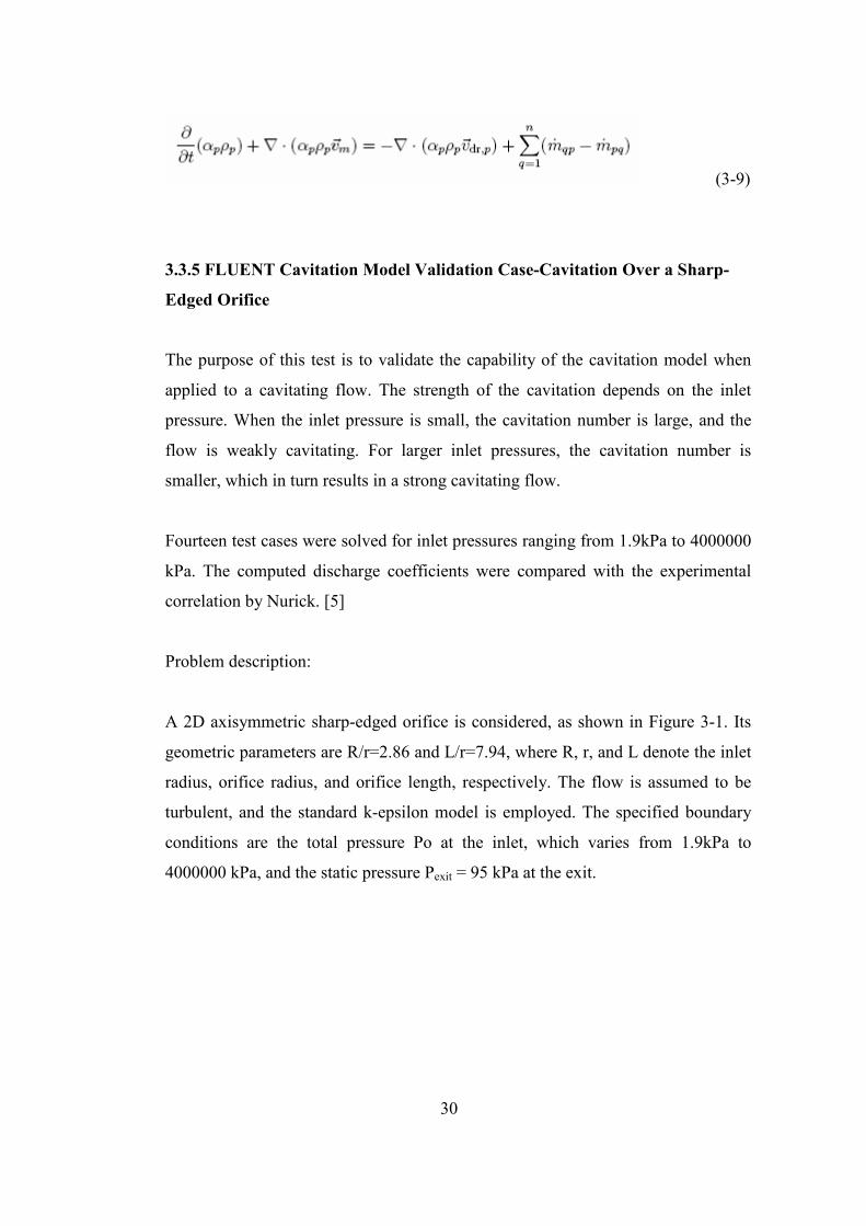
3.3.5 FLUENT Cavitation Model Validation Case-Cavitation Over a Sharp-

Edged Orifice

The purpose of this test is to validate the capability of the cavitation model when

applied to a cavitating flow. The strength of the cavitation depends on the inlet

pressure. When the inlet pressure is small, the cavitation number is large, and the

flow is weakly cavitating. For larger inlet pressures, the cavitation number is

smaller, which in turn results in a strong cavitating flow.

Fourteen test cases were solved for inlet pressures ranging from 1.9kPa to 4000000

kPa. The computed discharge coefficients were compared with the experimental

correlation by Nurick. [5]

Problem description:

A 2D axisymmetric sharp-edged orifice is considered, as shown in Figure 3-1. Its

geometric parameters are R/r=2.86 and L/r=7.94, where R, r, and L denote the inlet

radius, orifice radius, and orifice length, respectively. The flow is assumed to be

turbulent, and the standard k-epsilon model is employed. The specified boundary

conditions are the total pressure Po at the inlet, which varies from 1.9kPa to

4000000 kPa, and the static pressure Pexit = 95 kPa at the exit.

31

Figure 3-1. FLUENT Validation Case Geometry

Results:

Experimental data is available in the form of discharge coefficient versus cavitation

number, where the discharge coefficient is defined as idealmm••

/ , •

m is the computed

mass flow rate, and idealm•

is the ideal mass flow rate through the orifice. The ideal

mass flow rate through the orifice is computed as )(2 exitinth PPAm −=•

ρ , where Ath is

the cross-sectional area of the orifice, Ath=πr2, ρ is the density, and Pin and Pexit are

the inlet pressure and the exit pressure, respectively. At this solution the version of

the FLUENT is 6.2.5 and 2D solver is used.

32

Figure 3-2. FLUENT Validation Case Results

In Figure 3-2, Fluent results are in great agreement with the experimental results.

Also for the cavitating venturi case the previous test performed in TÜBĐTAK-

SAGE, in agreement with the Fluent results, which was shown in Figure 1-10.

In Figure 3-3, one of the results of the Fluent validation case was plotted. In this

case the inlet pressure is 50 bars.

33

a) Volume fraction of liquid water

b) Pressure distribution in (Pa)

c)Velocity distribution (m/s)

d) Grid resolution (7350 cells)

e) Grid at the throat section zoomed

Figure 3-3. Results for the FLUENT validation case at 50 bar inlet pressure.

Mesh dependency is also evaluated for the validation case. For 50 bar case the

cavitation numbers for three different mesh sizes is given in Table 3-1. The percent

difference between the solutions are calculated w.r.t. the results of the finest mesh

which has 56400 cells. The difference is calculated by using equation 3-10.

34

( )100

3_

3__

meshD

meshDkmeshD

C

CCABS − . (3-10)

Table 3-1. Mesh Size Versus Cavitation Number for FLUENT Validation Case at

50 bars

Mesh Size (cells) Discharge Coefficient Percent Difference

3525 (original) 0.631 1.28 %

14100 0.626 0.48 %

56400 0.623 0.00 %

35

CHAPTER 4

EXPERIMENTAL STUDY

Although the experiments are difficult to perform it is necessary to validate the

numerical simulation tools. Due to the complex flow behavior of cavitation it is

very difficult to perform experiments. Most of the parameters to be measured like

mass flow rate and pressure are the integral parameters that average the chaotic

flow field behavior. To investigate the flow field in details, local parameters have

to be measured but in such a chaotic environment it is difficult to do so. Therefore,

visualization techniques have to be used in order to investigate the flow field

without affecting the fluid flow. However in such a case, the test pressure and the

design of the test section gain importance. Pressure can not exceed specific values

due to stress limits in such visual materials. Although all cavitating venturies are

axis-symmetric, for better visual observability, two-dimensional test sections can

be used to understand the flow structure. Throughout this thesis several

axisymmetric and 3-D prismatic venturi geometries are tested. And the effect of

this difference is investigated in Chapter 5 in details.

4.1 Experimental Setup

In Figure 4-1, a simple sketch of the experimental setup is illustrated. Two high

pressure nitrogen tanks are used to pressurize the water tanks. One is used to define

the inlet pressure, P1, and the other is used to set the outlet pressure, P2. To regulate

the pressure, two high pressure-high flow rate pressure regulators are used. Also

two high pressure tanks are used to store the water. An additional needle valve is

attached to the water tank at the exit of the test section because the pressure

regulators work only one-way, therefore these regulators can not release the high

pressure gas to reduce the pressure. To prevent the pressure rise in the outlet due to

36

the decrease in volume of the water tank at the exit a needle valve is attached and

set to a value to get required pressure values. Also a solenoid valve operated ball

valve is used to separate the two pressurized zones before the experiment starts.

More over, two high pressure transducers attached to the proper locations like inlet

of the test section and to the exit of the test section. Here an additional pressure

sensor is not attached to the exit tank because the relief valve sets the outlet

pressure to the required value. To measure the mass flow rate through the test

section a turbine type flow meter is used. The pressure and the mass flow rate data

is collected with a data acquisition system and send to the computer.

Figure 4-1. Test Setup Sketch

4.1.1 Test Section

There are two different set of test sections are designed and produced. For the

preliminary tests four different axisymmetic venturi sections are used. These are

the configurations which are more physically similar to the real venturies. However

in these test the visibility of the bubble formation at the throat of the venturi is

affected from the shape of the venturi. The other set of test sections is designed to

be 3-D prismatic so that the core section of the venturi can be seen and this will be

better for comparison with the numerical flow solutions.

37

4.1.1.1 Axisymmetric Test Sections

First set of test is done with axisymmetric venturi geometries. In total four different

axisymmetric venturi geometries are manufactured. And the geometric properties

are given in Table 4-1. Due to the manufacturing difficulties, a blur region at the

throat section of the venturi remains in one of the venturies. Although wax is

applied to the inside of the venturi the best visual quality which is achieved can be

seen on Figure 4-2. The technical drawings of the cavitating venturies are given in

Appendix A-1

Table 4-1. Geometric Properties of the Axisymmetric Venturies

Din Dth Din/Dth Lth Lth/Din Ф1 Ф2

1 10 mm 5 mm 0.5 3 mm 0.3 30 deg 7 deg

2 10 mm 5 mm 0.5 3 mm 0.3 15 deg 15 deg

3 10 mm 5 mm 0.5 3 mm 0.3 15 deg 30 deg

4 10 mm 5 mm 0.5 3 mm 0.3 15 deg 60 deg

38

Figure 4-2. Pictures of the Tested Cavitating Venturies.

4.1.1.1 3-D Prismatic Test Section

To observe the cavitation process, venturi test section designed to be a 2-D cut of a

common axisymmetric venturi. From the previous tests it is known that it is very

hard to investigate the core flow and the fluctuations of the bubbles in an

axisymmetric Plexiglas venturi because of the manufacturing errors. Therefore a 3-

D prismatic test section designed to reduce the effect of these errors on

visualization. But there exists some difficulties because of the shape. The pipelines

connecting the test section with the pressurized tanks have circular cross-sections

but the test section inlet and outlet have to be rectangular. To change the flow

cross-section without disturbing the flow is done by additional adaptors, which the

technical drawings and the pictures are given in Appendix A-1.

39

4.2 Measurements

4.2.1 Pressure Measurements

Pressure is one of the main parameter has to be measured to calculate the cavitation

number. At least two high pressure transducers are necessary to investigate the

flow field. One is in front of the venturi and the second one has to be placed after

the venturi to calculate the P2 in the cavitation number. An additional pressure

transducer can be used to measure the throat pressure to ensure the cavitation.

However, due to the sensitivity of cavitation at the throat this measurement will

affect the characteristics of the cavitating venturi.

4.2.2 Mass Flow Rate Measurements

The main reason of the usage of the cavitating venturi is to limit or control the flow

rate of the working fluid. Therefore, it is necessary to measure mass flow rate. In

our experiments, to measure the flow rate a turbine type flow meter is used.

4.2.3 Visual Observations

A high speed camera is used to understand the bubble formation and dynamics of

flow. The camera is capable of recording at 4000 fps in black & white.

Figure 4-3. Picture of high speed camera

40

CHAPTER 5

RESULTS & DISCUSSIONS

The results obtained from numerical simulations and from the experiments are

given in this chapter. Numerical simulations are performed for 2-D, 2-D

Axisymmetric and 3-D prismatic cases. 2-D and 3-D prismatic venturi geometries,

which are employed in the experiments, are used to investigate the differences from

the 2-D axisymmetric venturi flows. The numerical solutions are also carried out to

investigate the wall effects on the test section. The experimental results are also

presented and compared with the numerical solutions.

5.1 Numerical Solutions

Numerical solutions are first aimed at investigating the effect of several parameters

on the performance of venturi flows, and correlating them with a theoretical

understanding. The correlations may then be used to further reduce the number of

simulations. The venturi flows are investigated parametrically by forming a

solution matrix based on the geometric variables of a venturi.

5.1.1 Numerical Solution Matrix

For a cavitation venturi, there are four basic geometric parameters: the inlet angle,

outlet angle, Dth/Din and Lth/Din. Among them the inlet angle and the outlet angle

are the most important parameters on cavitating venturi flows, and these two

parameters are assigned five different values in the solution matrix (Table 5-1). In

the literature [1] the optimum inlet and outlet angles are given as 15-18 degrees and

6-8 degrees, respectively. The inlet angles are taken as 7, 5, 30, 90 degrees. In

addition, a smooth curved venturi inlet which is widely used in industry is also

41

added to the list. The exit angles vary from 7 to 15, 30, 60, 90 degrees. Dth/Din ratio

and Lth/Din ratios are varied between two different values. Dth/Din ratio value also

defines the Reynolds number of the flow. Because, in most of the piping systems

Din is kept constant and the throat diameter is a restricted value to achieve the target

mass flow rate for a specific inlet pressure and exit pressure. The last parameter is

the cavitation number, “σ”, which has three different values. Length of the throat

and throat diameter is non-dimensionalized with the inlet diameter because of the

similarity of the orifice flow with the cavitating venturi flow.

All these parameters are chosen such that the values are corresponding to

meaningful dimensional numbers. Because fluent is a dimensional solver and in all

solution the inlet diameter is chosen to be 22.4mm (1”) which is a very common

value for pipe engineers. And the throat values which are used in solutions are

8mm and 16 mm respectively. The length of the throat is chosen to be 5mm and 10

mm in dimensional domain, and also due to the pressure regulation on Plexiglas

test section. The cavitation number values are chosen for 30 bar inlet pressure with

1 bar, 10 bar and 20 bar exit pressures, for the case which Dth/Din=0.357 and 7.2

bar inlet pressure with 0.25 bar, 2.4 bar and 4.8 bar exit pressure, for the case

which Dth/Din=0.714. Also to investigate the effect of Reynolds number on the

oscillation frequency of the cavitation bubble, inlet pressure increased to 60 bars

for the case which Dth/Din=0.357, but to keep the cavitation numbers fixed,

backpressures for these cases are modified as 3 bars, 20 bars and 40 bars

respectively for σ1, σ2 and σ3. For the case which Dth/Din=0.714, inlet pressure is

increased to 30 bars and the exit pressures 1 bar, 10 bar and 20 bar respectively for

σ1, σ2 and σ3 to keep the cavitation number fixed. A summary of the solution

matrix and a simple sketch of the venturi with the parameters shown are given in

Figure 5-1 and Table 5-1 below.

42

Figure 5-1. Geometric Parameters are Given on a Generic Venturi

Table 5-1. Solution Matrix for Numerical Solutions

Inlet Angle Ф1 (deg) Outlet Angle Ф2 (deg) Dth/Din Lth/Din σ

Curved 7 0.357 0.223 1.0336

7 15 0.714 0.446 1.4988

15 30 2.9979

30 60

90 90

Turbulence Effects:

Since FLUENT recommends k-e model for cavitation calculations, all calculations

was made with this turbulence model. (To calculate the Turbulence intensity,

hydraulic diameter values are used. Hd & Tu)

Turbulence intensity is assumed to be 5% through the solutions. And the hydraulic

diameter value is taken to be the maximum diameter of the test section.

43

Sample Venturi Solution:

Numerical solutions obtained from a generic venturi are given in Figure 5-2, 5-3, 5-

4, 5-5 and 5-6.

Pressure Contours:

In Figure 5-2, Static pressure distribution through a generic venturi solution is

plotted. Through the throat section liquid is accelerated till the vapor pressure of

water is reached. After that point although the flow is a mixture of the liquid and

vapor phases, at the cross sections which has bubble the pressure is equal to vapor

pressure.

Figure 5-2. Pressure (Pa) Field Through a Generic Venturi

44

Velocity Contours:

Figure 5-3 shows how the velocity increases through the throat section of the

venturi. This velocity can be calculated with simple 1-D equations.

Figure 5-3. Velocity (m/s) Field Through a Generic Venturi

Phase Volume Fraction Contours:

Formation and diffusion of the gas phase at the throat section of the venturi is given

in Figure 5-4. And in Figure 5-5 the vena contracta region can be seen. The

thickness of the gas phase region at the throat defines the discharge coefficient of

specific venturi geometry. The effect of boundary layer is reduced on the liquid

core of the throat because of the formation of the gas phase at the walls through the

throat section. This leads to a more uniform velocity profile through the throat

section and allows us to use simple Bernoulli equation on such complex flow

fields.

45

Figure 5-4. Liquid Phase Volume Fraction for a Generic Venturi

Figure 5-5. Liquid Phase Volume Fraction for a Generic Venturi Throat

46

Multiphase Mach Number Contours:

In Figure 5-6, Mach contours are plotted for a generic sample venturi flow solution.

The speed of sound for multiphase flow is calculated with equation 5-1. It can be

seen that at the throat section the Mach number is equal to 1 and the venturi is

effectively chocked.

( )( ) ( ) ( )

+

−+−

=

22

11

1

llgg

lgaa

a

ρα

ρα

αρρα

(5-1)

Figure 5-6. Mach Contour Plot for a Generic Venturi

47

5.1.2 2D-Axisymmetric Solutions

Through the numerical simulations effect of several parameters are investigated on

the performance of the venturi. These parameters are inlet angle, outlet angle, ratio

of length of throat to inlet diameter, ratio of throat diameter to inlet diameter,

cavitation number and Reynolds number. Also there are two basics effect of these

parameters exits. One is the on the discharge coefficient Cd and the other is the

effect of Strouhal number on the oscillation frequency of the cavitating bubble.

Each effect can be listed as follows

• Effect of Inlet Angle on Discharge Coefficient

• Effect of Outlet Angle on Discharge Coefficient

• Effect of Lth/Din & Dth/Din on Discharge Coefficient

• Effect of Reynolds Number on Discharge Coefficient

• Effect of Outlet Angle “Ф2” on oscillation frequency of the Cavitation

Bubble

• Effect of Dth/Din & Lth/Din ratio on oscillation frequency of the Cavitation

Bubble

• Effect of Reynolds Number on oscillation frequency of the Cavitation

Bubble

These effects will be discussed in details in the following sections.

For 2-D axisymmetric case the solution matrix will be same as in Table 5-1 except

there are additional solutions for different Reynolds numbers are present. For

solutions which performed for Dth/Din=0.357 case, Re numbers are 6E5 and 9E5.

And for Dth/Din=0.714 Re numbers are 6E6 and 1.2E6.

48

5.1.2.1 Effect of Inlet Angle “Ф1” on Discharge Coefficient “Cd”

The effect of inlet angle “Ф1” on the discharge coefficient “Cd” is given in Figure

5-11 and 5-12. In these figures, through the rows the outlet angle“Ф2”is constant

and through the columns length of the throat is constant.

For a cavitating venturi if the flow is choked the discharge coefficient is not a

function of the cavitation number. But for the cases which the cavitation does not

occur the discharge coefficient is smaller than the cavitating ones. This is because

the discharge coefficient is defined to be the ratio of ideal mass flow rate to the real

one. The ideal mass flow rate is calculated by writing the Bernoulli equation

between the throat and the inlet of the venturi. At the throat the limiting pressure is

the vapor pressure of the working fluid. And for a smaller value of pressure the

velocity at the throat is smaller than the cavitating one. Then the mass flow rate is

going to be smaller than the cavitating case mass flow rate.

In the light of the discussions in the previous paragraph from Figure 5-11 and

Figure 5-12 it can be seen than with the increasing inlet angle the discharge

coefficient is decreasing for all three σ values. And for small Ф1 (7 deg < Ф1)

values due to small bubble formation at the throat section, cavitation is affected

more when the outlet angle Ф2 is higher than 15 degrees for σ3. Even for 60 and 90

degrees of exit angle, the cavitation is affected at σ2 also. This is because the

cavitating region does not find a place to stay on high exit angles and if this

couples with the small bubble formation at the throat, the cavitation stops. (Figure

5-7). This phenomenon does not account for the case with a higher throat diameter

ratio. This can be due to the high momentum of the flow at throat which pushes the

back pressure further downstream and keeps the flow cavitating.

49

Figure 5-7. Flow Path Lines Colored with Phase Volume Fractions for Case σ2.

5.1.2.2 Effect of Outlet Angle “Ф2” on Discharge Coefficient “Cd”

If the flow is cavitating the discharge coefficient is not a function of the outlet

angle “Ф2”. In Figure 5-13 & 5-14, it can be seen that for all cases with different

throat lengths and different throat diameters if the flow cavitates at the throat, with

the increasing exit angle the discharge coefficient is constant. But the exit angle

defines if the cavitation exists for high cavitation numbers or not, because the exit

angle defines the position of the cavitation bubble for a specific exit pressure. If the

outlet angle is not sufficiently small to give space to bubble to hold on a section in

the diffuser, the pressure wave at the exit moves back in to the throat of the venturi

and stops cavitation. That’s why only the venturies with outlet angle less than 15

degrees are cavitated for σ3 values, which means small differential pressures. Also

this angle defines the oscillation frequency of the cavitation bubble but this will be

discussed on the following sections.

5.1.2.3 Effect of Lth/Din & Dth/Din on Discharge Coefficient “Cd”

It is very interesting to see in Figure 5-19 & 5-20, that the ratio of throat length to

inlet diameter and the ratio of throat diameter to inlet diameter do not affect the

discharge coefficient at all. Just for the case with inlet angle 90 degrees, the effect

50

of throat diameter ratio is interesting. The difference is also stated in orifice flow

equations in the literature. But for lower inlet angles this effect disappears rapidly.

5.1.2.4 Effect of Reynolds Number on Discharge Coefficient “Cd”

It is known that for a cavitating venturi, if the venturi cavitates the discharge

coefficient is a fixed value for all inlet pressures for a prescribed geometry. But in

Figure 5-25 & 5-26 one can see that for all cases with the increasing Reynolds

Number for small inlet angles (Curved and 7 degree) the discharge coefficient is

increasing. This effect disappears with the increasing inlet angle. This phenomenon

can be caused by the effect of momentum which pushes the vapor part at the throat

to the wall of the throat. This will increase the effective core area and as a

consequence of this the discharge coefficient increase. Also the Reynolds number

has an effect on the unstable oscillating bubble frequency value but this will be

discussed further.

5.1.2.5 Effect of Outlet Angle “Ф2” on oscillation frequency of the cavitation

bubble

When a cavitation bubble created at the throat of the venturi it diffuses to the

downstream of the venturi and diffusion stops at a specific length. With the

increasing cavitation number, the position of the bubble moves to upstream. This

position is not always a stable point but oscillates between two arbitrary points on

the diffuser of the venturi. These oscillations seen only for the venturies which has

outlet angle less than 30 degrees. Over this value the diffuser length is getting

smaller and the bubble is not able to stay on a stable position.

The oscillations of the bubble on a venturi can be seen in Figure 5-8. In this figure

one period of the fluctuations are plotted. Also the variations on the exit mass flow

rate caused by these fluctuations are given in Figure 5-9. Figure 5-10 is rather

interesting; it is believed that when the cavitation occurs at the throat of the venturi

than the flow is chocked so that the pressure waves at the exit can not be

51

transmitted to the upstream of the throat section. However, in Figure 5-10 the

fluctuations on the inlet mass flow rate can be seen. Although these fluctuations are

very small for this venturi, in some cases the magnitude of these fluctuations may

rise as 50 % of the inlet mass flow rate. In Figure 5-8 at time 0.140s the core of the

flow at the throat exit has the values of 0.85 to 0.9 phase volume fraction. The

velocity of sound in such heterogeneous medium at some regions will increased so

that at these points the Mach number is not equal to 1 anymore.

In Table B-2, it can be seen that the Strouhal number for a venturi, which has same

Dth/Din and the Lth/Din, is a function of the outlet angle.

52

t=0.000s

t=0.002s

t=0.004s

t=0.006s

t=0.008s

t=0.10s

t=0.012s

t=0.014s

Figure 5-8. Variation of the Volume Fraction of Vapor Phase for Sample Venturi

Geometry at σ2.

53

Figure 5-9. Unsteady Oscillation at the Exit Plane of the Venturi.

Figure 5-10. The Effect of Oscillating Cavitation Bubble on the Inlet Mass Flow

Rate.

54

5.1.2.6 Effect of Dth/Din & Lth/Din ratio on oscillation frequency of the

cavitation bubble

Although the Reynolds Number and the Cavitation number are similar for

venturies, the oscillation behavior can be different. The cases where Dth/Din = 0.714

the flow do not oscillates for any of the venturies. Which can be a consequence of

the effect of different diffuser lengths of the venturies for the same geometric

parameters. With the decreasing diffuser length the bubble can not be stay at the

diffuser section.

The throat length has a different effect on the oscillation behavior, it does not affect

the value of oscillation frequency but it reduces the oscillation magnitude at the

inlet section. With the increasing throat length the bubbles which are produced at

the throat inlet wall can cover the core of the throat at a smaller distance. This

effect increases the volume fraction of vapor phase and reduces the fluctuations at

the inlet mass flow.

5.1.2.7 Effect of Reynolds Number on oscillation frequency of the cavitation

bubble

For relatively low Reynolds number flows the effect of viscous terms and the

Reynolds stress terms become more significant. These terms tends to damp the

unsteady oscillation in the cavitation bubble [9]. In table B.2, the Strouhal numbers

calculated for several oscillation cases are given. Although the Strouhal number is

decreasing the frequency of the oscillations are increasing in the solutions.

5.1.2.8 Summary of 2-D Axisymmetric Solutions

Through the axisymmetric solutions, parameters which thought to be effective on

the performance of the cavitating venturi are given in previous sections. These can

divided in to two main parts. One is the effects on the discharge coefficient and the

55

other is effects on the oscillation frequency. From the discussions it can be seen

that the discharge coefficient is only a function of inlet angle and Reynolds

number. But the effect of Reynolds number is almost negligible. And the exit angle

defines the cavitation performance of the venturi and the oscillation frequency of

the cavitation bubble. The effect of Lth/Din is only seen on the inlet oscillations of

the cavitating venturies. A longer throat gives a sufficient length to mixture to be

homogenous through the throat of the venturi. But this does not change the

frequency of the oscillation at the diffuser part. Dth/Din ratio is one of the important

parameter like in orifice flow, with the increasing throat diameter; the diffuser

length is getting smaller compared to the one which has a smaller throat diameter

for the same exit angle. And these effects the oscillation and cavitation behavior of

the venturi due to the effect describes in related section in details.

5.1.3 2-D Solutions

During the experiments a 3-D prismatic section of the cavitating venturi is used.

Therefore, the effect of this selection has to be investigated before the experiments.

Because of time limitations, 2-D solutions are performed instead of 3-D solutions.

These 2-D solutions are performed on the test matrix given in Table 5-1, but for a

fixed Reynolds number, Re=6E6. The effect of several parameters are investigated

such that;

• Effect of inlet angle on Discharge Coefficient

• Effect of outlet angle on Discharge coefficient

• Effect of Lth/Din & Dth/Din on Discharge Coefficient “Cd”

• Effect of Outlet Angle “Ф2” on oscillation frequency of the cavitation

bubble

, and given in the following sections.

For 2-D solutions the solution matrix given in Table 5-1 and the solutions are

performed for Reynolds number equal to 6E5.

56

5.1.3.1 Effect of Inlet Angle “Ф1” on Discharge Coefficient “Cd”

The effect of the inlet angle on discharge coefficient is not different from the 2-D -

Axisymmetric and 2-D cases accept for the case which have a higher Dth/Din

diameter value. For the axisymmetric case for these Dth/Din ratios and for σ3 the

cavitation occurred for the outlet angle values below 15 degrees. This is because of

the difference between the volume expansions of these two cases. For the

axisymmetric case the expansion area increases with the square of the radius but

for the 2D case area increases just linearly. Also for the exit angles 60 & 90

degrees at σ2 condition for Dth/Din=0.357, the effect of back pressure on cavitation

is not seen as in axisymmetric case. This can be a consequence of the volume

expansion difference also.

5.1.3.2 Effect of Outlet Angle “Ф2” on Discharge Coefficient “Cd”

For 2D case the effect of outlet angle “Ф2” on the discharge coefficient is smaller.

The cavitation will continue till the outlet angle increased to 30 degrees at σ3 for

Dth/Din = 0.357. But for the case which has a larger throat diameter, small area

expansion can not be able to hold the back pressure at the diffuser part. The effect

can be seen in Figure 5-12.

5.1.3.3 Effect of Lth/Din & Dth/Din on Discharge Coefficient “Cd”

The effects are same as in axisymmetric solutions.

5.1.3.4 Effect of Outlet Angle “Ф2” on oscillation frequency of the cavitation

bubble

Two dimensional solutions show quite different oscillation behavior from 2-D

axisymmetric case. For all 2-D solutions the oscillation is damped out. This

damping may caused by the effect of volume ratio or the definition of the Reynolds

number. For both 2-D and 2-D axisymmetric cases the characteristic length is

57

defined as Dth therefore the Reynolds number is same for both cases. But the

volume extension at the diffuser part is not same. So this may lead such a different

behavior on the oscillation charteristics of 2-D solutions.

5.1.3.5 Summary for 2-D results

In discharge coefficient point of view, 2-D and 2-D axisymmetric results have

almost same values for every possible venturi geometry but the oscillation

charteristics are very different from each other. This yields to the result that 2-D

venturi sections can be used to obtain discharge coefficient but the limiting

cavitation value, where the cavitation stops, and oscillation frequencies can not be

simulated with 2-D sections.

58

Lth/Din=0.223 Lth/Din =0.446

Ф2=90

Ф2=60

Ф2=30

Ф2=15

Ф2=7

Figure 5-11. Discharge-Coefficient (Cd) vs. Ф1 for 2D –Axisymmetric Solutions at

Re=6E5 for Dth/Din=0.357

59

Lth/Din=0.223 Lth/Din =0.446

Ф2=90

Ф2=60

Ф2=30

Ф2=15

Ф2=7

Figure 5-12. Discharge-Coefficient (Cd) vs. Ф1 for 2D –Axisymmetric Solutions at

Re=6E5 for Dth/Din =0.714

60

Lth/Din=0.223 Lth/Din =0.446

Ф1=90

Ф1=30

Ф1=15

Ф1=7

Ф1=Curved

Figure 5-13. Discharge-Coefficient (Cd) vs. Ф2 for 2D –Axisymmetric Solutions at

Re= 6E5 for Dth/Din=0.357

61

Lth/Din=0.223 Lth/Din =0.446

Ф1=90

Ф1=30

Ф1=15

Ф1=7

Ф1=Curved

Figure 5-14. Discharge-Coefficient (Cd) vs. Ф2 for 2D –Axisymmetric Solutions at

Re= 6E5 for Dth/Din=0.714

62

Lth/Din=0.223 Lth/Din =0.446

Ф2=90

Ф2=60

Ф2=30

Ф2=15

Ф2=7

Figure 5-15. Discharge-Coefficient (Cd) vs. Ф1 for 2D Solutions at Re=6E5 for

Dth/Din=0.357

63

Lth/Din=0.223 Lth/Din =0.446

Ф2=90

Ф2=60

Ф2=30

Ф2=15

Ф2=7

Figure 5-16. Discharge-Coefficient (Cd) vs. Ф1 for 2D Solutions at Re=6E5 for

Dth/Din=0.714

64

Lth/Din=0.223 Lth/Din =0.446

Ф1=90

Ф1=30

Ф1=15

Ф1=7

Ф1=Curved

Figure 5-17. Discharge-Coefficient (Cd) vs. Ф2 for 2D Solutions at Re=6E5 for Dth/Din=0.357

65

Lth/Din=0.223 Lth/Din =0.446

Ф1=90

Ф1=30

Ф1=15

Ф1=7

Ф1=Curved

Figure 5-18. Discharge-Coefficient (Cd) vs. Ф2 for 2D Solutions at Re=6E5 for Dth/Din=0.714

66

Dth/Din=0.357 Dth/Din =0.714

Ф1=90

Ф1=30

Ф1=15

Ф1=7

Ф1=Curved

Figure 5-19. Effect Lth/Din on Discharge-Coefficient (Cd) vs. Ф2 for 2D-Axisymmetric Solutions at σ1

67

Lth/Din=0.223 Lth/Din =0.446

Ф1=90

Ф1=30

Ф1=15

Ф1=7

Ф1=Curved

Figure 5-20. Effect Dth/Din on Discharge-Coefficient (Cd) vs. Ф2 for 2D-Axisymmetric Solutions at σ1

68

Dth/Din=0.357 Dth/Din =0.714

Ф1=90

Ф1=30

Ф1=15

Ф1=7

Ф1=Curved

Figure 5-21. Effect Lth/Din on Discharge-Coefficient (Cd) vs. Ф2 for 2D Solutions at σ1

69

Lth/Din=0.223 Lth/Din =0.446

Ф1=90

Ф1=30

Ф1=15

Ф1=7

Ф1=Curved

Figure 5-22. Effect Dth/Din on Discharge-Coefficient (Cd) vs. Ф2 for 2D Solutions at σ1

70

Lth/Din=0.223 Lth/Din =0.446

Ф2=90

Ф2=60

Ф2=30

Ф2=15

Ф2=7

Figure 5-23. 2D- Axisymmetric Solutions vs. 2D Solutions for Dth/Din=0.357 at σ1

71

Lth/Din=0.223 Lth/Din =0.446

Ф2=90

Ф2=60

Ф2=30

Ф2=15

Ф2=7

Figure 5-24. 2D- Axisymmetric Solutions vs. 2D Solutions for Dth/Din=0. 0.714 at

σ1

72

Lth/Din=0.223 Lth/Din =0.446

Ф2=90

Ф2=60

Ф2=30

Ф2=15

Ф2=7

Figure 5-25. Reynolds Number Effect on Discharge Coefficient on Axisymmetric

Venturi Flows for Dth/Din=0.357 at σ1

73

Lth/Din=0.223 Lth/Din =0.446

Ф2=90

Ф2=60

Ф2=30

Ф2=15

Ф2=7

Figure 5-26. Reynolds Number Effect on Discharge Coefficient on Axisymmetric

Venturi Flows for Dth/Din=0. 0.714 at σ1

74

5.1.4 Effect of the Wall Depth

Because the 3-D prismatic test section is used in the experiments, the wall has a

certain effect on the flow and bubble dynamics because of the boundary layer

formation on the walls. This effect is investigated with FLUENT in order to see the

effect on the discharge coefficient and oscillation behavior. To reduce the effect, it

is better to use a very deep test section but due to limitation on the pipe size and the

difficulty of changing the pipe circular section to rectangular section the depth have

to be optimized. Also the high pressure tank which is used in the experiments has a

limited volume and with the increasing depth, the flow rate can be much higher

than expected and this will reduce the experiment time.

75

a1 ) 5 mm depth

a2) 5 mm depth

b1) 10 mm depth

b2) 10 mm depth

c1) 15 mm depth

c2) 15 mm depth

Figure 5-27. Effect of Wall for 3-D Prismatic Solutions at σ1.

In Figure 5-27, the 3-D Prismatic solution obtained for three different depth values

is plotted. And in Figure 5-28 the discharge coefficient obtained from 2-D, 2-D

axisymmetric and 3-D prismatic solutions plotted for three different cavitation

number. And it can be seen that the discharge coefficient does not affected too

much from the walls and the difference does not exceeds 1 - 2 % from each other.

76

Figure 5-28, Discharge Coefficient vs. 2-D, 2-D Axisymmetric and 3-D Prismatic

Solutions.

Table 5-2. Oscillation Frequency for 2-D, 2-D Axisymmetric and 3-D Prismatic

Solutions

f (Hz) σ1 f (Hz) σ2 f (Hz) σ3

2-D - - -

2-D Axisymmetric - 80 92

3-D Prismatic(5 mm) - - 61.7

3-D Prismatic(10 mm) - - 62.1

3-D Prismatic(15 mm) - - 62.8

Also the oscillation charcteristics are compared. In Table 5-2 the oscillation

frequencies are given for the same venturi geometry for three different cavitation

numbers. And it is very interesting to see that the oscillation occurs at 3-D

prizmatic and 2-D axisymmetric case but not in 2-D solutions. Also the oscillation

frequency of 3-D and 2-D axisymmetric solution is different but this frequency

value is consistent with in 3-D prismatic solutions.

77

5.1.5 Summary for Numerical Simulations

Through out the numerical simulations 100 different venturi geometries solved for

three cavitation number values at two different Reynolds number for both 2-D

axisymmetric and 2-D cases. Test number reduction techniques could not be

applied to the numerical simulation due to the lack of empirical equations which

correlates the geometric features of the venturi with the flow variables. The output

of the simulations is the discharge coefficient “Cd”, which defines the efficiency,

and the oscillation frequency of the exit mass flow rate.

From the simulations it can be seen that exit angle “Ф2“, Lth/Din ratio and

Cavitation number “σ” do not have any effect on the discharge coefficient “Cd”.

Although Dth/Din value affects the discharge coefficient for high inlet angles the

sole effect is due to the inlet angle value, which is correlated as in equation (5-2).

9726.00064.00066.00006.000003.0 121 +

−Φ

−

+Φ=

in

th

in

thd

D

D

D

DC (5-2)

In case of oscillations at the exit mass flow rate and the critical cavitation number,

the exit angle “Ф2“ and the Dth/Din ratio are the main parameters because of the fact

that they are directly define the diffuser length of the venturi.

In the plots of several venturi simulations an arc is present in the phase volume

fraction contours on the axis of the venturi. (Figure 5-5 & Figure 5-26). This may

caused by a numerical error while defining the axis boundary condition at the axis

of venturi.

78

5.2 Experimental Results

5.2.1 Experiment Matrix

For the experiments four different axisymmetric venturi geometries and a 3-D

prismatic venturi test section is designed and manufactured. Through the

axisymmetic venturi tests the objective is to see the effect of outlet angle on the

critical cavitation number and on the frequency of the fluctuations at the exit

pressure. Therefore several experiments are performed for different cavitation

numbers.

79

5.2.2 Experiments with Axisymmetric Venturi Flows

In the experiments, a total of 8 flow cases with 3 different venturies were studied.

In the first 3 cases, the inlet and exit angles are set at Ф1 = 30deg, Ф2 = 7deg,

respectively, and the back pressure was varied for cavitation numbers in the range

of 1-4. Similarly in Cases 4 and 5, where Ф1 = 15deg, Ф2 = 15 deg, and in Cases 6-

8, where Ф1 = 15 deg, Ф2 = 60 deg, the backpressure was varied to assess the

cavitating flows. The flow features through the venture was captured by a high-

speed camera at 500 frames per second, and the pressure variations at the inlet and

exit sections were measured using pressure transducers at a sampling rate of

5000Hz. The flow rate in the experiments could not be measured due the low

response time of the flow meter used in the setup.

5.2.2.1 Case 1: Ф1 = 30 deg, Ф2 = 7 deg, σ=1

In this case the inlet pressure is set to Pin=22bars (gage) and the exit pressure is set

to Pout=0bars. As seen in Figure 5-30(a), as soon as the valve is opened, the exit

pressure drops to -1 bar and remains constant. At t=2500 ms, the valve is closed,

and the exit pressure recovers the inlet pressure. The fluctuations observed after the

valve is closed are attributed to the water hammer effect produced as a result of

rapid closing of the valve. The drop in the inlet pressure, which is about 10 bars, is

due to the poor regulation of the gas pressure in the water tank. The variation of the

cavitation number during the experiment is given in Figure 5-30(b). Since the exit

pressure is 0 bars, the cavitation number remains constant.

80

Figure 5-29. High Speed Camera Plot

a)

b)

Figure 5-30. a) Pressure vs. Time b) Cavitation Number vs. Time

Core section

81

5.2.2.2 Case 2: Ф1 = 30 deg, Ф2 = 7 deg, σ=2

In case 2, it is observed in high speed camera pictures (Figure 5-31) that the

cavitation in the venturi disappears at about t = 1200 ms, which is attributed to the

increase in the cavitation number (Figure 5-32(b)). After the cavitation number

reaches a value of about 4, the cavitation stops.

The presence of the pressure fluctuations shown in Figure 5-32(a) also indicates the

cavitation. The high frequency movement of the bubble in the diffuser part causes

the pressure fluctuation at the exit region. It is apparent that the sole source of the

pressure fluctuations is the cavitating flow though venturi.

The frequency analysis of the exit pressure variation indicates the significant

modes, one is about 400-450 Hz and the other is about150-250 Hz (Figure 5-32(c)).

82

t= 215 ms

t= 1039 ms

t= 319 ms

t= 1453 ms

t= 333 ms

t=1601 ms

Figure 5-31. High Speed Camera Plots

83

a)

b)

c)

Figure 5-32.a) Pressure vs. Time b) Cavitation Number vs. Time

c) PSD vs. Frequency (Hz)

84

5.2.2.3 Case 3: Ф1 = 30 deg, Ф2 = 7 deg, σ=1.2-1.8

In this case the exit pressure is set to Pout=12bars and initial inlet pressure is set to

Pin=34bars. The frequency content of the exit pressure fluctuations changes through

the experiment due to the change in the cavitation number (Figure 5-33 (b) & (d)).

With the increasing cavitation number, the back pressure pushes the cavitation

bubble upward direction through the diffuser and this upstream motion gives less

space to the bubble to collapse. Therefore the frequency of the fluctuations

increases with the increasing cavitation number. But the amplitude of the

fluctuations decreases. In Figure 5-33 (c) the range of fluctuation in the exit

pressure are about 100-150 Hz and 400-450 Hz at the beginning of the experiment.

Through the experiment with the increasing cavitation number the lower frequency

fluctuations tend to be disappearing. Also these low frequency oscillations can be

calculated from the high speed camera plots which are given in Figure 5-34. From

this figure if the one period of the fluctuations is assumed to be between t=710 to

718 and t=720 to 730 the frequency of this fluctuations can calculated as between

100-125, which can be seen on the waterfall diagram given in Figure 5-33(d).

85

a)

b)

c)

d)

Figure 5-33. a) Pressure vs. Time b) Cavitation Number vs. Time c) PSD vs.

Frequency (Hz) d) Waterfall Diagram of Exit Pressure

86

t=710 ms

t=720 ms

t=712 ms

t=722 ms

t=714 ms

t=724 ms

t=716 ms

t=730 ms

t=718 ms

Figure 5-34. High Speed Camera Plots

87

5.2.2.4 Case 4: Ф1 = 15 deg, Ф2 = 15 deg, σ=1.4-1.7

In this case the back pressure is set to Pout=8 bars and the inlet pressure is set to

Pin=30 bars. Through the experiment the cavitation number kept under 2. (Figure 5-

35 (b)). The pressure fluctuations at the exit plane are damped out with the

increasing cavitation number in this experiment also. The amplitudes of the

oscillations in the inlet pressure are more than the previous venturies. This shows

that the inflow is not fully uncoupled with the exit pressure for cavitation number

which is closer to critical cavitation number. Also in Figure 5-35(c) it can be seen

that the oscillations exits in the range 200-275 Hz.

88

a)

b)

c)

Figure 5-35. a) Pressure vs. Time b) Cavitation Number vs. Time c) PSD vs.

Frequency

89

t=244 ms

t=900 ms

t=1007 ms

t=1185 ms

Figure 5-36. High Speed Camera Plots

90

5.2.2.5 Case 5: Ф1 = 15 deg, Ф2 = 15 deg, σ=1.5-2.0

In case 5, an almost constant cavitation is achieved through the experiment. In

figure 5-37 (a), the effect of the exit pressure on the inlet pressure is more visible in

this experiment. Through the experiment the cavitation number is kept under 2 so

that the cavitation is continuous. Again the power spectrum density plots shows

that the oscillations are take place in the range of 200-350Hz. This shows a

similarity with the previous experiment for this venturi.

a)

b)

c)

Figure 5-37. Pressure vs. Time b) Cavitation Number vs. Time c) PSD vs.

Frequency

91

t=425 ms

t= 996 ms

t= 1181 ms

Figure 5-38. High Speed Camera Plots

92

5.2.2.6 Case 6: Ф1 = 15 deg, Ф2 = 60 deg, σ=1.2-1.4

In this case rather interesting results are obtained. In Figure 5-39 (a), the frequency

of the oscillations in the exit pressure changes with the rising cavitation number,

which is given in Figure 5-39(b). The cavitation number value is about 1.2 at the

beginning and increases to 1.4 at the end of the experiment. And with the

increasing cavitation number the oscillation frequencies are increased. Due to this

low cavitation numbers the effect of exit oscillations on the inlet pressure is

minimized.

a)

b)

c)

Figure 5-39. a) Pressure vs. Time b) Cavitation Number vs. Time c) PSD vs.

Frequency

93

t=203 ms

t=224 ms

t=1340 ms

t= 1359 ms

Figure 5-40. High Speed Camera Plots

94

5.2.2.7 Case 7: Ф1 = 15 deg, Ф2 = 60 deg, σ=1.4-3.0

In Figure 5-41(a) the pressure variation obtained in case 7 is given. As it is

observed the cavitation occurs between t=200-1250 ms where the cavitation

number is less than 2. Also in Figure 5-41 (c) the frequency of the fluctuations is

seen to be in the range of 200-350 Hz.

a)

b)

c)

Figure 5-41. a) Pressure vs. Time b) Cavitation Number vs. Time c) PSD vs.

Frequency

95

t= 450 ms

t=1060 ms

t=1400 ms

Figure 5-42. High Speed Camera Plots

96

5.2.2.8 Case 8: Ф1 = 15 deg, Ф2 = 60 deg, σ=1.0

In this case the exit pressure is set to be 0 bars, which sets the cavitation number to

1. As seen in Figure 5-43 (a), pressure fluctuations do not exist anymore, which

indicates that the bubble formed in the diffuser is stable and stays stationary. The

two-phase flow in the core region is similarly stable. (Figure 5-43 (c)).

a)

b)

c)

Figure 5-43. a) Pressure vs. Time b) Cavitation Number vs. Time c) High Speed

Camera Plot

97

5.2.3 Previous Engine Tests in TÜBITAK-SAGE

In Figure 5-44. The pressure variation in the combustion chamber obtained from an

engine test is given. Based on the results presented above, the high amplitude

oscillations at about 250-300 Hz, which could not be explained then, can now be

attributed to the cavitating venturi flows.

Figure 5-44. Engine Combustion Chamber Pressure Data.

98

Figure 5-45. Engine Combustion Data Frequency Analysis.

5.2.4 Failure in the Experiments with 3-D Prismatic Venturis

Experiments with 3-D prismatic venturi flows were not successful due to the

failure of the test section. The venturi walls made of Plexiglas was broken under

the high pressure. Quick modifications to reduce the stress concentration at the

corners of the machined parts did not prevent the failure. These experiments were

therefore abandoned.

99

CHAPTER 6

CONCLUSION

In this work, cavitating venturi flows are investigated numerically and

experimentally. Some of the important parameters for cavitating venturi flow like

inlet, outlet angles, throat to inlet diameter ratio and length of throat to inlet

diameter ratio on discharge coefficient and cavitation behavior are investigated

also.

Through the numerical simulations 2-D, 2-D Axisymmetric and 3-D prismatic

cases are solved for several Reynolds number and cavitation number values.

Results shown that the 2-D and 2-D axisymmetric results are almost having the

same discharge coefficients but when in case of oscillations the behavior is

different from each other.

Through the experiments three different axisymmetric venturi geometries with

different inlet and outlet angles are tested for several cavitation numbers. Due to

the problems related to the pressure regulators the inlet pressure can not be kept

constant in the experiments but this gives us a chance to investigate the flow at

different cavitation numbers. Also the flow meter can not be used in the

experiments because of the delay in the response of the flow meter. The first set of

experiments shows that the cavitating venturi flow is highly turbulent and three-

dimensional. These three-dimensional effects change the frequency of the

oscillations. In the numerical simulations because the cavitation modeled as an

axisymmetric, the frequency range in rather low. But in the real world these high

momentum bubbles can not be survive through the end of the diffuser. These

bubbles are collapsed and roll over each other and break down in to smaller

bubbles. These low momentum bubbles creates a higher frequency oscillation with

100

a smaller amplitude in the exit pressure. Also in the numerical simulations the

static back pressure is fixed at the exit plane therefore the mass flow rate changes

during the simulation. But in the experiments the back pressure can not be fixed.

If we compare the result of the numerical simulations and the experiments, in

general we can say that the main parameter like discharge coefficient and critical

cavitation number can be foreseen with the FLUENT flow solver. But in the case

of oscillation frequency prediction, a more complex three-dimensional flow

solution is necessary and may be in the future LES turbulence model can be used to

simulate this unsteady creation and collapse of the bubbles in the venturies.

101

REFERENCES

[1] J. FOX, “Modeling Cavitating venturies”, 1970

[2] J. A. BOURE, A. A. FRITTE, M. M. GIOR and M. L. REOCREUX,

“Highlights of Two-Phase Critical Flow: On the Links Between Maximum Flow

Rates, Sonic Velocities, Propagation and Transfer Phenomena in Single and Two-

Phase Flows”, Int. J. Multiphase Flow Vol. 3, pp. 1-22, 1974

[3] K.H.ARDRON and R. B. DUFFEY, “Acoustic Wave Propagation In a Flowing

Liquid-Vapour Mixture”, Int. J. Multiphase Flow Vol. 4, pp. 303-322, 1978

[4] K. H. ARDRON, “A Two-Fluid Model For Critical Vapor-Liquid Flow”, Int. J.

Multiphase Flow Vol. 4,pp. 323-337, 1978

[5] N. T. THANG and M.R. DAVIS, “Pressure Distribution in Bubbly Flow

Through Venturis”, Int. J. Multiphase Flow Vol. 7, pp. 191-210, 1981

[6] Guston and Reises

[7] J.D. SHERWOOD, “Potential Flow Around a Deforming Bubble In a Venturi”,

International Journal of Multiphase Flow26, 2000

[8] GUILLERMO PALAU SALVADOR AND STEVEN H. GRANKEL,

“Numerical Modeling of Cavitation Using FLUENT: Validation and Parametric

studies”,34th AIAA Fluid Dynamics Conference and Exhibit 28 June -1 July 2004,

Portland, Oregon, AIAA 2004-2642

[9] Changhai XU, Stephen D. HEISTER and Robert FIELD, “Modeling Cavitating

Venturi Flows”,

[10] E. ELIAS and G.S. LELOUCHE, “Two-Phase Critical Flow”, Int. J.

Multiphase Flow Vol. 20, pp. 91-168, 1994

[11] DAVID P. SCHMIDTH, CHRISTOPHER J. RUTLAND, and M. L.

CORRADINI, “A Fully Compressible, Two-Dimensional, Model of Small, High

Speed, Cavitating Nozzles”, 1985

102

[12] Y. YAN AND R. B. THORPE, “Flow Regime Transition Due to Cavition In

The Flow Through An Orifice”, Int. J. Multiphase Flow Vol. 16, No. 6, pp. 1023-

1045, 1990

[13] C. E. BRENNEN, “Cavitation And Bubble Dynamics”, Oxford Engineering

Science Series, ISBN 13:978-0-19-509409-1

[14] FLUENT User Manual

103

APPENDIX A

EXPERIMENTAL SETUP TECHNICAL DRAWINGS &

MEASURMENT EQUIPMENT

A.1 Technical drawings of experimental setup

104

105

106

107

108

109

A.2 Specifications of transducers, data acquisition system, high speed camera

and valves, regulators.

A.2.1 Data Acquisition system

IOTECH Dacbook 2000E

• 16 Channel Analog input

• 200kHz data acquisition capacity from one channel

• 16 Channel Thermocouple extension

Figure A2-1. Data Acqusition System

110

A.2.2 Pressure Transducers

Kistler 701 a quartz pressure sensor for measuring dynamic and quasistatic

pressures up to 250 bars.

Figure A2-2. Pressure Transducer

A.2.3 Flow Meter

Hoffler turbine type high pressure flow meter.

Figure A2-3.Hoffler Turbine Type Flow Meter

111

A.2.5 Pressure Regulator

HOKE High pressure (0-400) bars high flow pressure regulator

Figure A2-4. Pressure Requlator

112

APPENDIX B

RESULTS OF NUMERICALS SIMULATIONS

B.1 Temperature vs. Vapor Pressure Table

Taken from the Sonntag, Borgnakke and Van Wylen, “Fundamentals of

Thermodynamics”, 1998, John Wiley & Sons

Table B-1. Vapor Pressure vs. Temperature.

Temperature C° Vapor Pressure (Pa)

0,01 611,3

5 872,1

10 1227,6

15 1705

20 2339

25 3169

30 4246

35 5628

40 7384

45 9593

50 12350

55 15758

60 19941

65 25030

70 31190

75 38580

80 47390

85 57830

90 70140

95 84550

100 101300

105 120800

110 143300

115 169100

113

Figure B-1. Vapor Pressure of Water vs. Temperature

Figure B-2. Strouhal Number vs. Outlet Angle

114

Figure B-3. CAD Drawing of the Test Section and the Adaptors.

Figure B-4.Parts of the 3-D Prismatic Test Section

115

Figure B-5. Assembly of the 3-D Prismatic Test Section

Figure B-6.Four Different Venturi Configuration for 3-D Prismatic Test Section

CAD drawing of the test section is given in Figure B-2. The test section consists of

a Plexiglas visual section, a holder for the 3-D prismatic venturi sections at the

back of the visual section and two tightening plates and two flow adaptors which

are placed at the inlet and the outlet of the test sections. Plexiglas test section is

produced with milling method to reduce the leakage from the joints. The technical

drawings of the test section are given in Appendix A-1.

116

Table B-2. Geometric Properties of the Venturies for 3-D Prismatic Test Section

Din Dth Din/Dth Lth Lth/Din Ф1 Ф2

1 22.4 mm 8 mm 0.357 5 mm 0.223 15 deg 7 deg

2 22.4 mm 8 mm 0.357 5 mm 0.223 30 deg 7 deg

3 22.4 mm 8 mm 0.357 5 mm 0.223 15 deg 15 deg

4 22.4 mm 16 mm 0.714 5 mm 0.223 15 deg 15 deg

117

B.2 Results of 2-D Axisymmetric Simulations

Table B-3. Results of 2-D Axisymmetric Numerical Simulations

118

119

120

121

For 2D case

Table B-4. Results of 2-D Numerical Simulations at Re=6E5

Ф1 Ф2 Dth/Din Lth/Din Cd-σ1 Cd- σ2 Cd- σ3 Stin(σ2) Stin(σ3) Stout(σ2) Stout(σ3)

1 Curved 7 0.357 0.223 0.912 0.912 0.912 c c c 0.000 0.000 0.000 0.000 2 7 7 0.357 0.223 0.933 0.933 0.933 c c c 0.000 0.000 0.000 0.000 3 15 7 0.357 0.223 0.895 0.895 0.000 c c c 0.000 0.000 0.000 0.000 4 30 7 0.357 0.223 0.825 0.825 0.825 c c c 0.000 0.000 0.000 0.000 5 90 7 0.357 0.223 0.654 0.654 0.653 c c c 0.000 0.000 0.000 0.000 6 Curved 15 0.357 0.223 0.911 0.911 0.910 c c c 0.000 0.000 0.000 0.000 7 7 15 0.357 0.223 0.933 0.933 0.931 c c c 0.000 0.000 0.000 0.000 8 15 15 0.357 0.223 0.894 0.894 0.891 c c c 0.000 0.000 0.000 0.000 9 30 15 0.357 0.223 0.824 0.824 0.820 c c c 0.000 0.000 0.000 0.000 10 90 15 0.357 0.223 0.655 0.655 0.611 c c - 0.000 0.000 0.000 0.000 11 Curved 30 0.357 0.223 0.909 0.909 0.841 c c - 0.000 0.000 0.000 0.000 12 7 30 0.357 0.223 0.933 0.933 0.854 c c - 0.000 0.000 0.000 0.000 13 15 30 0.357 0.223 0.895 0.895 0.847 c c - 0.000 0.000 0.000 0.000 14 30 30 0.357 0.223 0.825 0.825 0.810 c c c 0.000 0.000 0.000 0.000 15 90 30 0.357 0.223 0.654 0.654 0.575 c c - 0.000 0.000 0.000 0.000 16 Curved 60 0.357 0.223 0.912 0.912 0.745 c c - 0.000 0.000 0.000 0.000 17 7 60 0.357 0.223 0.655 0.655 0.551 c c - 0.000 0.000 0.000 0.000 18 15 60 0.357 0.223 0.895 0.895 0.763 c c - 0.000 0.000 0.000 0.000 19 30 60 0.357 0.223 0.823 0.823 0.725 c c - 0.000 0.000 0.000 0.000 20 90 60 0.357 0.223 0.934 0.934 0.755 c c - 0.000 0.000 0.000 0.000 21 Curved 90 0.357 0.223 0.912 0.912 0.721 c c - 0.000 0.000 0.000 0.000 22 7 90 0.357 0.223 0.933 0.933 0.729 c c - 0.000 0.000 0.000 0.000 23 15 90 0.357 0.223 0.894 0.894 0.729 c c - 0.000 0.000 0.000 0.000 24 30 90 0.357 0.223 0.824 0.824 0.707 c c - 0.000 0.000 0.000 0.000 25 90 90 0.357 0.223 0.655 0.655 0.545 c c - 0.000 0.000 0.000 0.000 26 Curved 7 0.714 0.223 0.900 0.900 0.761 c c - 0.000 0.000 0.000 0.000 27 7 7 0.714 0.223 0.934 0.934 0.771 c c - 0.000 0.000 0.000 0.000 28 15 7 0.714 0.223 0.894 0.894 0.768 c c - 0.000 0.000 0.000 0.000 29 30 7 0.714 0.223 0.842 0.842 0.746 c c - 0.000 0.000 0.000 0.000 30 90 7 0.714 0.223 0.729 0.729 0.633 c c - 0.000 0.000 0.000 0.000 31 Curved 15 0.714 0.223 0.898 0.898 c c - 0.000 0.000 0.000 0.000 32 7 15 0.714 0.223 0.934 0.934 0.769 c c - 0.000 0.000 0.000 0.000 33 15 15 0.714 0.223 0.895 0.895 0.768 c c - 0.000 0.000 0.000 0.000 34 30 15 0.714 0.223 0.833 0.833 0.740 c c - 0.000 0.000 0.000 0.000 35 90 15 0.714 0.223 0.727 0.698 0.613 c c - 0.000 0.000 0.000 0.000 36 Curved 30 0.714 0.223 0.901 0.901 0.735 c c - 0.000 0.000 0.000 0.000 37 7 30 0.714 0.223 0.934 0.934 0.743 c c - 0.000 0.000 0.000 0.000 38 15 30 0.714 0.223 0.896 0.896 0.742 c c - 0.000 0.000 0.000 0.000 39 30 30 0.714 0.223 0.834 0.834 0.722 c c - 0.000 0.000 0.000 0.000 40 90 30 0.714 0.223 0.720 0.720 0.590 c c - 0.000 0.000 0.000 0.000 41 Curved 60 0.714 0.223 0.901 0.901 0.693 c c - 0.000 0.000 0.000 0.000 42 7 60 0.714 0.223 0.934 0.934 0.701 c c - 0.000 0.000 0.000 0.000 Cont’d

122

Ф1 Ф2 Dth/Din Lth/Din Cd-σ1 Cd- σ2 Cd- σ3 Stin(σ2) Stin(σ3) Stout(σ2) Stout(σ3)

43 15 60 0.714 0.223 0.897 0.897 0.700 c c - 0.000 0.000 0.000 0.000 44 30 60 0.714 0.223 0.835 0.835 0.687 c c - 0.000 0.000 0.000 0.000 45 90 60 0.714 0.223 0.724 0.724 0.589 c c - 0.000 0.000 0.000 0.000 46 Curved 90 0.714 0.223 0.901 0.901 0.704 c c - 0.000 0.000 0.000 0.000 47 7 90 0.714 0.223 0.934 0.000 0.713 c c - 0.000 0.000 0.000 0.000 48 15 90 0.714 0.223 0.895 0.895 0.712 c c - 0.000 0.000 0.000 0.000 49 30 90 0.714 0.223 0.832 0.832 0.693 c c - 0.000 0.000 0.000 0.000 50 90 90 0.714 0.223 0.722 0.722 0.593 c c - 0.000 0.000 0.000 0.000 51 Curved 7 0.357 0.446 0.913 0.913 0.913 c c c 0.000 0.000 0.000 0.000 52 7 7 0.357 0.446 0.934 0.934 0.934 c c c 0.000 0.000 0.000 0.000 53 15 7 0.357 0.446 0.895 0.895 0.895 c c c 0.000 0.000 0.000 0.000 54 30 7 0.357 0.446 0.824 0.824 0.824 c c c 0.000 0.000 0.000 0.000 55 90 7 0.357 0.446 0.654 0.654 0.654 c c c 0.000 0.000 0.000 0.000 56 Curved 15 0.357 0.446 0.911 0.911 0.911 c c c 0.000 0.000 0.000 0.000 57 7 15 0.357 0.446 0.935 0.935 0.935 c c c 0.000 0.000 0.000 0.000 58 15 15 0.357 0.446 0.894 0.894 0.894 c c c 0.000 0.000 0.000 0.000 59 30 15 0.357 0.446 0.823 0.823 0.823 c c c 0.000 0.000 0.000 0.000 60 90 15 0.357 0.446 0.656 0.656 0.654 c c c 0.000 0.000 0.000 0.000 61 Curved 30 0.357 0.446 0.910 0.910 0.834 c c - 0.000 0.000 0.000 0.000 62 7 30 0.357 0.446 0.934 0.934 0.843 c c - 0.000 0.000 0.000 0.000 63 15 30 0.357 0.446 0.894 0.894 0.847 c c - 0.000 0.000 0.000 0.000 64 30 30 0.357 0.446 0.824 0.824 0.813 c c c 0.000 0.000 0.000 0.000 65 90 30 0.357 0.446 0.656 0.656 0.615 c c - 0.000 0.000 0.000 0.000 66 Curved 60 0.357 0.446 0.913 0.913 0.743 c c - 0.000 0.000 0.000 0.000 67 7 60 0.357 0.446 0.934 0.934 0.748 c c - 0.000 0.000 0.000 0.000 68 15 60 0.357 0.446 0.894 0.894 0.751 c c - 0.000 0.000 0.000 0.000 69 30 60 0.357 0.446 0.824 0.824 0.719 c c - 0.000 0.000 0.000 0.000 70 90 60 0.357 0.446 0.655 0.655 0.567 c c - 0.000 0.000 0.000 0.000 71 Curved 90 0.357 0.446 0.913 0.913 0.715 c c - 0.000 0.000 0.000 0.000 72 7 90 0.357 0.446 0.934 0.000 0.720 c c - 0.000 0.000 0.000 0.000 73 15 90 0.357 0.446 0.894 0.894 0.720 c c - 0.000 0.000 0.000 0.000 74 30 90 0.357 0.446 0.823 0.823 0.701 c c - 0.000 0.000 0.000 0.000 75 90 90 0.357 0.446 0.655 0.655 0.562 c c - 0.000 0.000 0.000 0.000 76 Curved 7 0.714 0.446 0.898 0.898 0.756 c c - 0.000 0.000 0.000 0.000 77 7 7 0.714 0.446 0.934 0.934 0.770 c c - 0.000 0.000 0.000 0.000 78 15 7 0.714 0.446 0.895 0.895 0.770 c c - 0.000 0.000 0.000 0.000 79 30 7 0.714 0.446 0.833 0.833 0.744 c c - 0.000 0.000 0.000 0.000 80 90 7 0.714 0.446 0.722 0.722 0.639 c c - 0.000 0.000 0.000 0.000 81 Curved 15 0.714 0.446 0.898 0.898 0.751 c c - 0.000 0.000 0.000 0.000 82 7 15 0.714 0.446 0.934 0.934 0.766 c c - 0.000 0.000 0.000 0.000 83 15 15 0.714 0.446 0.894 0.894 0.763 c c - 0.000 0.000 0.000 0.000 84 30 15 0.714 0.446 0.833 0.833 0.739 c c - 0.000 0.000 0.000 0.000 85 90 15 0.714 0.446 0.723 0.723 0.627 c c - 0.000 0.000 0.000 0.000 86 Curved 30 0.714 0.446 0.898 0.898 0.732 c c - 0.000 0.000 0.000 0.000 87 7 30 0.714 0.446 0.934 0.934 0.743 c c - 0.000 0.000 0.000 0.000 88 15 30 0.714 0.446 0.894 0.894 0.741 c c - 0.000 0.000 0.000 0.000 89 30 30 0.714 0.446 0.833 0.833 0.725 c c - 0.000 0.000 0.000 0.000 90 90 30 0.714 0.446 0.725 0.725 0.617 c c - 0.000 0.000 0.000 0.000 91 Curved 60 0.714 0.446 0.901 0.901 0.695 c c - 0.000 0.000 0.000 0.000 Cont’d

123

Ф1 Ф2 Dth/Din Lth/Din Cd-σ1 Cd- σ2 Cd- σ3 Stin(σ2) Stin(σ3) Stout(σ2) Stout(σ3)

92 7 60 0.714 0.446 0.934 0.934 0.700 c c - 0.000 0.000 0.000 0.000 93 15 60 0.714 0.446 0.894 0.894 0.699 c c - 0.000 0.000 0.000 0.000 94 30 60 0.714 0.446 0.833 0.833 0.689 c c - 0.000 0.000 0.000 0.000 95 90 60 0.714 0.446 0.723 0.723 0.610 c c - 0.000 0.000 0.000 0.000 96 Curved 90 0.714 0.446 0.898 0.898 0.701 c c - 0.000 0.000 0.000 0.000 97 7 90 0.714 0.446 0.934 0.934 0.712 c c - 0.000 0.000 0.000 0.000 98 15 90 0.714 0.446 0.894 0.894 0.710 c c - 0.000 0.000 0.000 0.000 99 30 90 0.714 0.446 0.833 0.833 0.696 c c - 0.000 0.000 0.000 0.000 100 90 90 0.714 0.446 0.723 0.723 0.610 c c - 0.000 0.000 0.000 0.000