Numerical and Laboratory Investigations for Maximization of Production from Tight/Shale Oil Reservoirs: From Fundamental Studies to Technology Development and Evaluation PROGRESS-END REPORT June 15, 2015 Task 1: Project management and planning This task aims to develop a plan for project management, and identify the researchers responsible for the various components of the study. Progress in Task 1: Work on Task 1 was completed ahead of schedule. G. Moridis was the Principal Investigator (PI), assisted by Matt Reagan (co-PI). T. Kneafsey was responsible for core-scale laboratory experiments, J. Ajo-Franklin was in charge of the nano-scale experiments and visualization, and G. Waychunas was in charge of the Molecular Fluid Dynamics Studies. G. Moridis and M. Reagan were responsible for the laboratory and field-scale simulations of shale oil production/recovery. Task 2: Definition of metrics and methodology for screening production strategies This task aimed to define the feasibility parameters, the specific objectives and metrics of the screening study, and the corresponding methodology for the evaluation of the various strategies to be investigated. This task included discussions among the members of the LBNL group, interactions with academia and discussions with industry specialists from companies with significant shale oil properties that are actively involved in low-viscosity fluid production from oil shale reservoirs. Progress in Task 2: Work on Task 2 was completed on schedule. Several internal discussions of the LBNL team have led to the identification (and quantification, where appropriate) of the parameters, objectives and metrics of the study, as well as the methodology. The first step involved the determination of the reference (base) cases, and the LBNL team decided that these have to be two: the first is the case of production from unfractured or naturally fractured reservoirs, and the second is that of production from a hydraulically (or pneumatically) fractured reservoir. The second reference case is expected to represent a significant improvement of production over that in the first reference case. The next issue the LBNL team considered was the definition of the concept of recovery under conditions of ultra-low permeability. Activities in this task involved discussions with researchers in industry and academia. After several iterations, the LBNL agreed on a definition of “success” of recovery of shale oil that involves an increase in production (rate or cumulative) of at least 50% higher than that realized in the 2 nd reference case (i.e., the one involving hydraulic or pneumatic fracturing) over a period that corresponds
Transcript
Numerical and Laboratory Investigations for Maximization of Production from Tight/Shale Oil Reservoirs: From Fundamental Studies to Technology
Development and Evaluation
PROGRESS-END REPORT June 15, 2015
Task 1: Project management and planning This task aims to develop a plan for project management, and identify the researchers responsible for the various components of the study. Progress in Task 1: Work on Task 1 was completed ahead of schedule. G. Moridis was the Principal Investigator (PI), assisted by Matt Reagan (co-PI). T. Kneafsey was responsible for core-scale laboratory experiments, J. Ajo-Franklin was in charge of the nano-scale experiments and visualization, and G. Waychunas was in charge of the Molecular Fluid Dynamics Studies. G. Moridis and M. Reagan were responsible for the laboratory and field-scale simulations of shale oil production/recovery. Task 2: Definition of metrics and methodology for screening production strategies This task aimed to define the feasibility parameters, the specific objectives and metrics of the screening study, and the corresponding methodology for the evaluation of the various strategies to be investigated. This task included discussions among the members of the LBNL group, interactions with academia and discussions with industry specialists from companies with significant shale oil properties that are actively involved in low-viscosity fluid production from oil shale reservoirs. Progress in Task 2: Work on Task 2 was completed on schedule. Several internal discussions of the LBNL team have led to the identification (and quantification, where appropriate) of the parameters, objectives and metrics of the study, as well as the methodology. The first step involved the determination of the reference (base) cases, and the LBNL team decided that these have to be two: the first is the case of production from unfractured or naturally fractured reservoirs, and the second is that of production from a hydraulically (or pneumatically) fractured reservoir. The second reference case is expected to represent a significant improvement of production over that in the first reference case. The next issue the LBNL team considered was the definition of the concept of recovery under conditions of ultra-low permeability. Activities in this task involved discussions with researchers in industry and academia. After several iterations, the LBNL agreed on a definition of “success” of recovery of shale oil that involves an increase in production (rate or cumulative) of at least 50% higher than that realized in the 2nd reference case (i.e., the one involving hydraulic or pneumatic fracturing) over a period that corresponds
to the economically productive life of a shale oil well. On current evidence, this period is expected to be in the 3 to 5 year range. Additionally, the LBNL team reached a conclusion that it is not possible to use a single metric/approach to quantify recovery. Thus, recovery in this study will no longer be represented by a single number or a range of numbers, but will instead be represented by a time-variable function of the following two quantities:
(a) As a fraction of the original oil-in-place of the volume of the reservoir subdomain defined by the well spacing (assuming standard horizontal wells)
(b) As a fraction of the original oil-in-place of the volume of the Stimulated Reservoir Volume (SRV - usually smaller than that defined by the well spacing)
Note that there other issues affecting these metrics of recovery (e.g., difficulties in describing drainage areas in heterogeneous systems), stage and cluster spacing, etc.), but it is expected that the complexities of these issues are attenuated over the chosen period of evaluation, i.e., 3-5 years. Task 3: Evaluation of enhanced liquids recovery using displacement processes In this task we evaluate by means of numerical simulation "standard" recovery strategies involving displacement processes, accounting for all known system interactions. The simulations were conducted using the TOUGH+MultiPhaseMultiComponent code (hereafter referred to as T+MpMc), a member of the family of codes developed at LBNL. T+MpMc was enhanced from the original version (Moridis and Blasingame, 2014) that had been available to the project since its inception with the addition of the most recent quantitative advances in fluid behavior in petroleum systems. The T+MpMc simulations focused on traditional continuous gas flooding using parallel horizontal wells and using the currently abundant shale gas, to the early exclusion of techniques such as (a) water-alternating-gas (WAG) flooding, and (b) huff-and-puff injection/production strategies using lean gas/rich gas in a traditional (single) horizontal well with multiple fractures. The concentration on continuous gas flooding was brought about by the results of the early simulations, which indicated a very large increase in pressures in the WAG case (easily exceeding the fracturing pressure of most geological media), and insignificant to practically no increase in production in both the WAG and huff-and-puff processes. Progress in Task 3: Work on Task 3 was completed ahead of schedule. Using properties and conditions that are typical of the Eagle Ford, Niobrara and Bakken formation (Table 1), we completed the investigation of displacement processes using N2, CH4 and He as the displacement gases using parallel horizontal wells (see Figures 1 and 2). The studies cover the spectrum of permeability between 1 nD and 1 µD, and consider a variety of fracture types (Figure 3). Note that Figure 3 shows the “stencils” of the four different fracture types (I to IV), i.e., the minimum repeatable subdomain that can accurately describe the well-and-reservoir system. Each stencil represents 1/8th of the full 3D domain between two hydraulic fractures and two parallel horizontal wells, and is the domain simulated in all the studies reported here. The consideration of the stencil as an adequate representation of the actual
system is based on the assumption of symmetry. This is a valid approximation (even for the lower part of the actual domain, despite the absence of consideration for the effects of gravity) because of the very limited gravitational contribution to the total pressure. Earlier studies (Olorode et al., 2013) had confirmed convincingly this approach. Figures 4 and 5 provide the results – the oil mass production rate Q and the corresponding cumulative mass M of the produced oil, respectively -- for two base (reference) cases, i.e., for an unfractured and a Type I fractured system (referred to as Cases R and RF, respectively). In both cases, a “dead oil”, i.e., oil containing with no dissolved gas, was considered. This indicates an assumption of a discovery pressure below the bubble point or a lack of gas, the latter being an indication of a relatively young age of the oil, i.e., the transformation of the kerogen in the source rock is still in the early “oil window (the “gas window”, being the later and final stage of transformation, has not been reached). A Type I fracture system (see Figure 3, characterized by the hydraulic fracture and the rock matrix) described by a dual permeability flow regime is considered in this study, which involves a 3D grid with very fine discretization that has 3.7x10⁵ elements and about 106 connections. Figures 4 and 5 show the effects of (a) the matrix permeability and (b) hydraulic fracturing in Cases R and RF. As expected, the early/initial oil mass production rate Q increases with an increasing matrix permeability k (later production is affected by the limited mass of the resource in the considered stencil domain). Additionally, Figures 4 and 5 show the dramatic effect of the hydraulic fracture on (early) production, which is consistent for all matrix permeabilities. A significant effort was invested in the evaluation of the production potential of “gassy oil”, i.e., oil with significant amounts of dissolved gas (mainly CH4) at the discovery pressure. This gas is exsolved (i.e., it evolves from solution) when the pressure in the reservoir drops below the bubble point. We used properties that are consistent of the gas-oil ratio in the Bakken (1000 SCF/bbl, and a bubble point Pb = 95% of the discovery/initial pressure), and we estimated gas production for (a) the range of matrix permeabilities considered in this study and (b) for an unfractured and a fractured (Type 1) reservoir. The results in Figure 6 show the superior recovery of “gassy” oil vs. that of “dead” oil in both an unfractured and a Type I fractured system. Although total recovery is the same because the amount of oil is fixed in the simulation stencil we consider, production of gassy oil is much faster for all matrix permeabilities and in both the R and RF Cases. Additionally, early recovery is enhanced by (a) the presence of fractures and (b) an increasing matrix permeability. The results of the oil-displacement studies in Figure 7 show very little (if any difference) in recovery between the two gases despite the affinity of CH4 for oil and the beneficial (for recovery) effects of density and viscosity reduction after CH4 dissolution into the oil (which were expected to enhance production). This is attributed to (a) difficulty in the slow, diffusion-dominated transport of CH4 through the displaced “bank” of oil to reach
virgin shale oil, and to (b) the limited effects that CH4 is expected to have in the “light” oil – octane -- considered here (the effect is much more pronounced in heavier oils). The effects of the study of He-based displacement of oil were practically identical to those of the N2 study. Note that these effects were obtained despite different diffusion coefficients of the 3 gases (in both the gas and the liquid phases), different Knudsen diffusion attributes, and even accounting for the effects of the dissolved gases (especially of CH4) on the oil density and viscosity. An important issue on which we have been investing significant effort is the discrepancy between simulation predictions and the larger recovery of oil observed during laboratory experiments (see the description and analysis in Appendix B). It should be noted that the laboratory study involved uniformly one-dimensional flow without any additional degree of freedom, and a much smaller scale. We began the simulations of the laboratory experiments in an effort to identify (by means of history-matching) the reasons for the discrepancies, which can be an issue of non-representative input values (a simpler problem) or the result of non-inclusion of important transport issues (a more complex problem, as it may involve unknown physics). At the end of this project, we had not concluded this study, but we had identified that the reasons for the significant differences were the estimates of gas permeability used in the computations of the lab experiments. It appears that it may not be appropriate to use a single “generic” gas permeability value, but a gas-specific one that may be linked to the gas molecular size. More study is needed to illuminate the issue, and whether the significant deviations in the recovery observations at the core scale persist (and to what degree) at the reservoir scale. The effect of a CO2-drive was also investigated. Such a process combines the elements of displacement with those of viscosity reduction, the latter resulting from the significant “swelling” effect of CO2 on oil. These were demanding simulations, with very long execution times. Figures 8, 9 and 10 summarize the effects of a CO2 drive on oil production (as quantified by the oil mass flow rate Q) on shale oil formations with matrix permeabilities of 10, 100 and 100 nD, respectively. These figures describe the CO2 on “dead” and “gassy” oil, as well as on unfractured and fractured (Type I) systems. Review of the figures indicate the universally positive effect of a CO2 drive in all cases: for both “dead” and “gassy” oil, and for both fractured and unfractured media. The enhancement of production is significant in all cases, but less significant than the effect of fracturing. In this task, a new semi-analytical solution to the problem of 3D flow through hydraulically fractured media was also developed. The new solution method is called the Transformational Decomposition Method (TDM), involves successive levels of transforms that eliminate time (Laplace transforms) and space (Finite Fourier transforms) from the original partial equations of flow through geologic media, are analytical in the multi-transformed space and semi-analytical in time and space, are applicable to heterogeneous systems (Figure 11) and are particularly well-suited to the study of production of liquids and gases from shales. TDM can be used to analyze well tests and to determine the flow properties of producing reservoirs. Verification and validation examples are shown in Figures 12 and 13. Figures 14 and 15 show respectively the pressure distribution and the curving stream lines corresponding to the 3D heterogeneous
problem used for verification in Figure 12. More details on the TDM solution are provided in Appendix A. Task 4: Evaluation of enhanced liquids recovery by means of viscosity reduction In this task we evaluate by means of numerical simulation (using the TOUGH+ family of codes developed at LBNL) the enhanced reservoir liquids recovery strategies that are based on viscosity reduction, accounting for all known system interactions. Such strategies will include (a) flooding using appropriate gases (e.g., CO2, N2, CH4) and appropriate well configurations (mainly horizontal), with the viscosity reduction resulting from the gas dissolution into the liquids, and (b) thermal processes, in which the viscosity reduction will be achieved by heating, possibly to the point of liquid vaporization and transport through the matrix to the production wells as a gas. Progress in Task 4: Work on Task 4 is ahead of schedule. The effect of viscosity reduction here is fully represented in the studies conducted in Task 3. Additionally, we have begun investigating the effects of thermal stimulation, effected by the flow of hot fluids through horizontal wells parallel to the actual production wells without actual injection into the formation. Such injections were dismissed as a possibility when preliminary scoping simulations showed (a) a very large pressure increase (caused by the low matrix permeability) that easily exceeded fracturing pressures of the rocks under consideration and (b) significant flow diversion of the injected fluids to the hydraulic fracture, thus leaving the bulk of the matrix unaffected. Preliminary results in Figure 16 indicate enhancement of production, but this occurs after a significant lead time. Early heating (described by Cases R_H2 and RF-H2 for a fractured and an unfractured system, respectively, which began 1 month before the onset of production) is more effective in increasing production that heating that begins at the time of the initiation of production (Cases R-H1 and RF-H1). In any case, (a) the increase in production appears to be a second-order effect (far less important than fracturing and CO2 displacement, and (b) it has to be further evaluated against the significant energy requirements to raise the temperature of the low-porosity, high-heat-capacity, low-thermal-conductivity shale system, considering that the dominant heat transport mechanism in shales is the slow diffusion. More studies on the subject are needed. Task 5: Multi-scale laboratory studies of system interactions The effort in this task focuses on the most promising approaches and methods identified in Tasks 2 and 3. Thus, oil-bearing samples of tight/shale formations (to be provided by Anadarko Petroleum, an industrial partner in this project) will be studied at various scales and under conditions corresponding to promising production methods. “Fresh” (i.e., recently recovered) representative media samples from at least two different reservoirs will be used. Progress in Task 5: In Task 5, samples received from an industrial collaborator in early February were deemed unsatisfactory because of excessive crumbling and age, which resulted in unacceptable quality. Following discussions and an agreement with
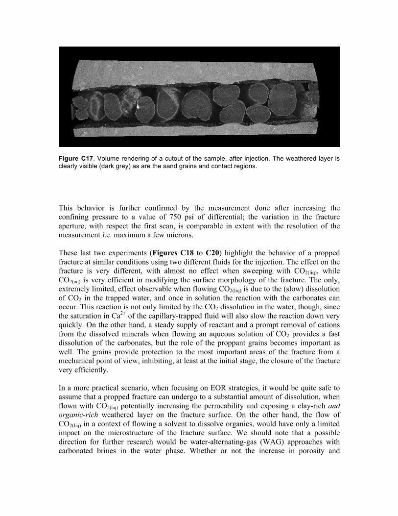
colleagues at the Colorado School of Mines, the LBNL team secured 400 lbs of fresh, high-quality Niobrara oil shales from an outcrop in Colorado. Appropriately sized samples of the Niobrara shales were subjected to a battery of tests: calibrated CT scans for core-scale density and heterogeneity analysis, scanning electron microscopic and X-ray powder diffraction for morphological characterization, mineralogy, chemical composition, microstructure and texture analyses. The experimental apparatus for core-scale studies has been designed and assembled. Following the completion of the laborartory apparatus, several sets of experiments were conducted. The first set involved oil displacement by means of supercritical CO2, and led to the redesign of the apparatus. The second set involved 44 experiments of depressurization and displacement using N2, CH4 and He, and provided very interesting results that indicated higher recovery than what our numerical simulations (using an admittedly different domain) had led us to expect. The study for the explanation of the discrepancy (and for determination of the cause) has progressed significantly, but could not be concluded given the budgetary and time constraints of this project. Among the interesting results of this study were (a) the distinct superiority/effectiveness of the CH4-based gas drive, compared to the N2 and He drives, and (b) the unexpectedly poor performance if the He-drive, which was shown to be the least effective despite the very small size of the He molecule. These results invalidated the assumption of He access to even the smallest pores and, consequently, a more effective oil displacement process. A detailed discussion of the experiments, procedure, results and analysis is provided in Appendix B. Finally, we secured in late 2015 and until May 2016 significant beam time at the Advanced Light Source facility of LBNL (the most powerful X-rays in the world) for the nano-scale study of pore-scale studies and oil flow analysis under a variety of recovery strategies. These studies were continuation of studied that began in April 2015. In addition to the characterization of the matrix rock and its fracturing attributes, the studies included micro-scale investigations and visualization of (a) fracture development during flow of carbonated water and (b) the effect of sweeping a propped fracture with liquid CO2. Among the most exciting results was the observation of significant “wormholing” and pitting of the shale by the advancing CO2, which results in increased porosity and permeability. This is the first such observation, and we expect that it may have a significant impact on the production effort. An additional unique new insight of this study was that the pitting does not appear to significantly weaken the mechanical strength of the rock at the fracture face, thus alleviating concerns about potential fast proppant embedment (and a consequent fracture aperture reduction or even closure) following a CO2 treatment. A detailed discussion of the micro-scale studies can be found in Appendix C. Task 6: Molecular simulation analysis of system interactions In this task, we study the expected fluid interactions and behavior in the most promising production scenarios identified in Tasks 2 and 3, as further focused by the results in Task 4. Such fluid systems may include either mobilized oil (e.g., after a thermal treatment), or combinations of the native oil and displacing fluids (e.g., liquid water, steam, CO2, CH4,
etc.) as well as kerogen and other high-viscosity hydrocarbons. Two types of molecular simulations are being used: Grand Canonical Monte Carlo (GCMC) simulations at constant temperature, chemical potential of the confined fluid, and pore volume, and classical Molecular Dynamics (MD) simulations at constant density (pressure) and temperature. Progress in Task 6: Work on Task 6 was completed on schedule. In a first approximation, we completed a realistic model of the pore structure using a simple slab and a cylindrical geometry. We will also develop a model of pore structure using the micro-CT data from a sample from the Niobrara formation (to be obtained from Task 5). These models allow us to obtain the thermodynamic phase behavior and fluid flow in a relatively straightforward manner as a function of the pore size. The intermolecular and intramolecular interactions are represented by effective force fields where the interaction energy is a function of intermolecular distance and several kinds of electrostatic interactions. Variations in electronic distribution are incorporated via charges placed at molecular sites. This method allows P-T phase diagrams to be computed directly from mixture isotherms obtained from GCMC simulations at various pressures, thus allowing one to estimate the conditions by which labile phase are present and in what proportion. Two significant advances have been achieved in the course of this study. The first involves the geometry: this is the first representation and simulation of a pore geometry, which exposes both basal planes and edges to interactions with the fluid molecules. The second advance is the first description of flow in porous media, as opposed to all previous studies that involved static (non-flowing) fluids in pores. This was achieved by to methods (a) enhanced flow-direction-oriented gravitational forces, and (b) fluid flow with a laminar velocity profile. The simulations that are currently in progress use the LAMMPS program running on the NERSC supercomputers at LBNL. The “oil” in these simulations is either pure n-C8 alkane, or a C8 alkane with substituent species (side chain, and benzene ring). A more detailed description of the activities on the subject can be found in Appendix D. Task 7: Evaluation of enhanced liquids recovery by means of increased reservoir stimulation, well design and well operation scheduling In this task, we evaluate numerically the effects of enhanced reservoir stimulation (e.g., using 20-25 stimulated wells per section) on the recovery of liquids by assessing (a) the performance of enhanced stimulation, (b) improved/appropriate well designs, and (b) the effects of appropriate operation scheduling/sequencing. Progress in Task 7: The substantial demands of the simulation effort assessing the impact of fracturing (natural and hydraulically induced), coupled with the limited budgetary resources available to the project, did not permit a significant effort in the direction of well design and operation. Thus, the bulk of the effort in this task focused on the effect of fracturing. Figure 17 shows the (significant) effects of the occurrence of natural fractures on production. The results of the studies in this task have indicated that that fractures (native or artificial/induced) have by far the largest positive impact on production.
References Moridis, G.J., and T.A. Blasingame, Evaluation of Strategies for Enhancing Production
of Low-Viscosity Liquids From Tight/Shale Reservoirs, Paper SPE 169479, 2014 SPE Latin America and Caribbean Petroleum Engineering Conference, 21-23 May, Maracaibo, Venezuela (http://dx.doi.org/10.2118/169479-MS).
Moridis, G.J., T. Blasingame and C.M.Freeman, Analysis of Mechanisms of Flow in
Fractured Tight- Gas and Shale-Gas Reservoirs, Paper SPE 139250, 2010 SPE Latin American & Caribbean Petroleum Engineering Conference, Lima, Peru, 1–3 December 2010.
Moridis, G.J., and C.M. Freeman, The RealGas and RealGasH2O Options of the
TOUGH+ Code for the Simulation Of Coupled Fluid And Heat Flow in Tight/Shale Gas Systems, Computers & Geosciences, 65, 56-71, 2014 (doi: 10.1016/j.cageo.2013.09.010).
Olorode, O.M., Freeman, C.M., G.J. Moridis, and T.A. Blasingame, High-Resolution
Numerical Modeling of Complex and Irregular Fracture Patterns in Shale Gas and Tight Gas Reservoirs, SPE Reservoir Evaluation & Engineering, 16(4), 443-455, 2013 (doi: 10.2118/152482-PA).
Stalgorova, K. and L. Mattar, Analytical Model for Unconventional Multifractured
Table 1 – Properties and conditions of the reference case (Type I)
Parameter Value Initial pressure P 2.00x10⁷ Pa (2900 psi) Initial temperature T 60 oC Bottomhole pressure Pw 1.00x10⁷ Pa (1450 psia) Oil composition 100% n-Octane
Initial saturations in the domain SO = 0.7, SA = 0.3 Intrinsic matrix permeability kx=ky=kz 10-18, 10-19, 10-20 m2 (=1000, 100, 10 nD)
Matrix porosity φ 0.05 Fracture spacing xf 30 m Fracture aperture wf 0.001 m
Fracture porosity φf 0.60 Formation height 10 m Well elevation above reservoir base 1 m Well length 1800 m (5900 ft) Heating well temperature TH 95 oC
SirA 1 λ 0.45 P0 2x10⁵ Pa Relative permeability Model17
krO = (SO*)n
krG = (SG*)n
SO*=(SO-SirO)/(1-SirA) SG*=(SG-SirG)/(1-SirA) EPM model
n 4
SirO 0.20 SirA 0.60
Figure 1 — Detailed stencil of the tight/shale reservoir investigated in the studies of Task 3 –View A.
Figure 2 — Detailed stencil of the tight/shale reservoir investigated in studies of Task 3 –View B.
I II
III IV Figure 3 — Clockwise: Stencils of Types I with a hydraulic fracture), II (hydraulic fracture and stress release fractures), III (hydraulic fracture and native/natural fractures) and IV (all types of fractures) fractured systems involving a horizontal well in a tight- or shale-gas reservoir (Moridis et al., 2010).
Figure 4 — Oil mass production rate Q in the reference Cases R (unfractured) and RF (fractured, Type I system), and effect of matrix permeability. A “dead oil” with no dissolved gas is assumed.
Figure 5 — Cumulative mass M of produced oil in the reference Cases R (unfractured) and RF (fractured, Type I system), and effect of matrix permeability. A “dead oil” with no dissolved gas is assumed.
Figure 6 — Effect of gas (CH4) dissolution on the cumulative mass M of produced oil in the reference Cases R (unfractured) and RF (fractured, Type I system) for various matrix permeabilities. The “dead oil” production is included for reference.
Figure 7 — Effect of a displacement process (gas drive using CH4 and N2) on the oil mass production rate Q. No discernible difference is observed between the production for CH4 and N2 drives.
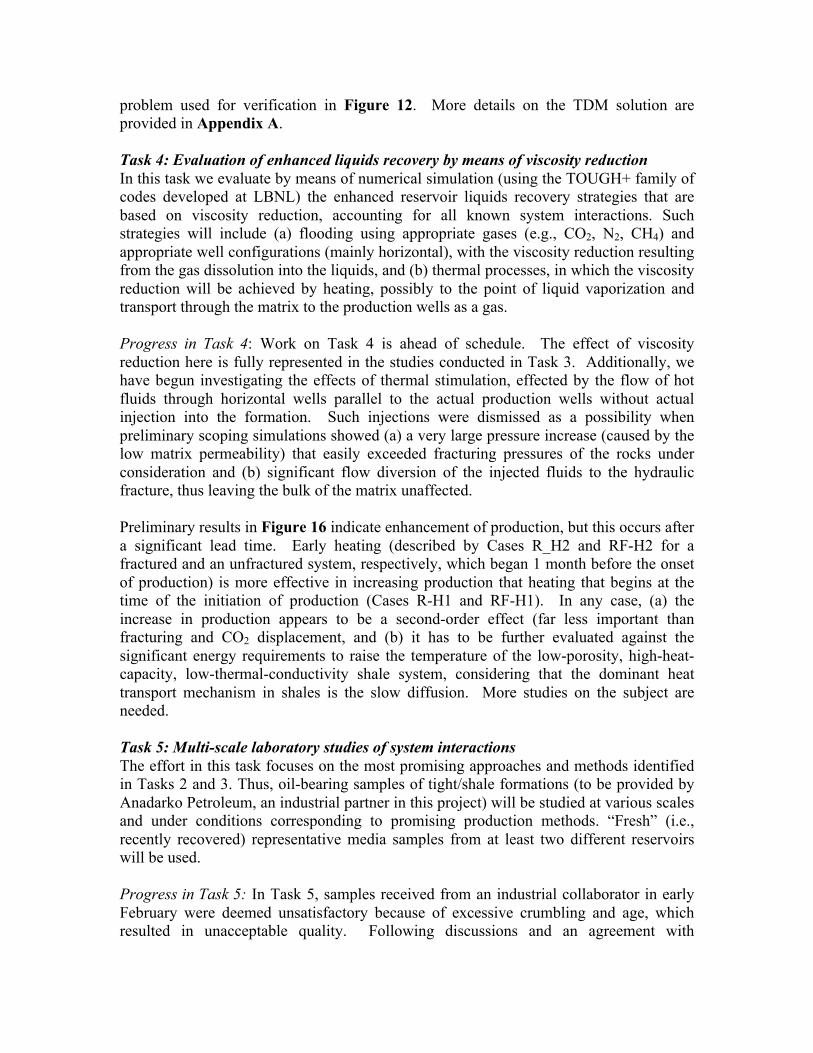
Figure 8 — Effect of a CO2-based displacement process on the mass rate Q of oil production for a matrix permeability of 10 nD. Both “dead” and “gassy” oil is considered in unfractured and fractured (Type I) systems.
Figure 9 — Effect of a CO2-based displacement process on the mass rate Q of oil production for a matrix permeability of 100 nD. Both “dead” and “gassy” oil is considered in unfractured and fractured (Type I) systems.
Figure 10 — Effect of a CO2-based displacement process on the mass rate Q of oil production for a matrix permeability of 1000 nD (= 1 µD). Both “dead” and “gassy” oil is considered in unfractured and fractured (Type I) systems.
Figure 11 — Symmetric quadrant (stencil) of a heterogeneous fractured oil reservoir (heterogeneity described by different intrinsic permeabilities k) for comparing the TDM model against results from a TOUGH+ numerical simulation.
Figure 12 — Comparison of the TDM solution to the simplified semi-analytical solution of Stalgorova and Mattar (2013).
Figure 13 — Comparison of the TDM solution to the TOUGH+RealGasH2O numerical simulator (Moridis and Freeman, 2014) in a complex 3D problem with the geometry of Figure 11.
Figure 14 — 3D pressure distribution from the TDM solution in the stencil shown in Figure 11. The TDM and the TOUGH+ solutions coincide.
Figure 15 — 3D stream lines from the TDM solution in the stencil shown in Figure 11. The curvature of the flow lines is fully described. The TDM and the TOUGH+ solutions coincide.
Figure 16 — Effect of heating on the mass rate of oil production Q.
Figure 17 — Effect of the presence of native fractures (NF) or similarly-acting secondary fractures on Q. The presence of fractures has the most pronounced positive effect on production.
APPENDIX A
Progress report: Semi-analytical simulation of reservoir with
heterogeneous permeability using Finite Fourier Transforms
J. K. Edmiston, G. J. Moridis
1 Summary
Low weight simulations at times may be preferable to setting up a large, high fidelity numericalsimulation where generating the correct input and interpreting output are complicated by the sizeof the simulation, in addition to computational costs. Many of the models designed for this areonly studied in the controlled production regime, which is inappropriate for unconventionals. Inthis note we build off the work of Stalgorova and Mattar [2] and Moridis [1] to investigate usingsimplified subdomain models of single phase porous flow in oil reservoirs to model production whenheterogeneous permeabilities due to hydraulic fracture are present. The method employs the FiniteFourier Transform in conjuction with Laplace transformation to obtain the solution at any desiredsimulation time instead of forward time integration. We have verified our simulation code againstboth literature and high resolution numerical solutions, for both types of production regimes.
2 Recent progress
We have verified our simulation method against those given in Figs 4, 9, and 10 of Stalgorova andMattar [2]. In that paper, a similar methodology to TD method is employed and shown to beapplicable to an important range of reservoir configurations with heterogeneous permeability. Inour comparison, we show that our alternative method as the benefit of being applicable to a widerrange of reservoir geometries at a cost of greater computational expense (though still less than ahigh fidelity numerical simulation).
To employ our method for the application, we used the three-dimensional subdomain decompo-sition shown in Figure 1, which shows 15 subdomain regions. By exploiting the z-symmetry aboutthe wellbore, we are able to reduce the domain size to 10 regions. Note that Stalgorova and Mattar[2] require only 5 regions. Each subdomain has a distinct permeability, either kfrac, k1, or k2, asindicated in Figure 1. The geometry and material parameters for the problems are displayed in Fig4 and Table 1 of Stalgorova and Mattar [2]. We note a typo that the listed production rate shouldbe 40 STB/D. Additionally, the width of the fractured region, w, is taken to be 0.25 in.
2.1 Results.
In Figures 2-4 we plot the well pressure pw vs. time for the cases shown in Figs 6, 9, and 10 of [2],respectively. To make an easier side by side comparison we make estimates of the data shown in therelevant figures of [2] - note that these are simply visually remapped data from their figures. Thefigures indicates a very favorable comparison with our method. We emphasize that the reservoir
1
Figure 1: Oil reservoir with heterogeneous permeability, adaptation from Stalgorova and Mattar[2, Fig. 4]. For values of the displayed parameters, consult Table 1 of [2].
geometries associated with Figure 3 and Figure 4 demonstrate better matching of numerical resultsthan their one-dimensional model.
2
0 200 400 600 800 1000
t[days]
0
2000
4000
6000
8000
10000
pw[psi]
TDMmethod
Stalgorova(2013),Fig.6
Figure 2: Well pressure pw vs time for the simulations given in Figs 6 of Stalgorova and Mattar [2].
0 2000 4000 6000 8000 10000 12000 14000 16000
t[days]
0
1000
2000
3000
4000
5000
pw[psi]
TDMmethod
Stalgorova(2013),Fig.9
Figure 3: Well pressure pw vs time for the simulations given in Fig 9 of Stalgorova and Mattar [2].
3
0 1000 2000 3000 4000 5000 6000 7000
t[days]
0
1000
2000
3000
4000
5000
pw[psi]
TDMmethod
Stalgorova(2013),Fig.10
Figure 4: Well pressure pw vs time for the simulations given in Fig 10 of Stalgorova and Mattar [2].
4
2.2 Pressure control boundary.
Next, we apply our method to an important boundary condition for unconventional tight oil reser-voirs, where we control the well pressure instead of production rate. The problem domain we useis depicted in Figure 5. The region has been reduced by symmetry to represent one quadrant of ahydraulic fracture stage. A 10 region model required by the cut out region for the horizontal welland single hydraulic fracture. The relative scale of the dimensions of the well are exaggerated forbetter depiction.
(a)
Figure 5: Symmetric quadrant of a fractured oil reservoir for comparing the TDM model againstTOUGH+.
2.3 Results - TOUGH+ comparison
Figure 6 compares the production for the TD method at various levels of discretization versusTOUGH+. The legend parameter N indicates the number of terms in each of the three coordinatesin the Fourier series expansion. We have approximately 10% error from the TOUGH+ solutionusing a coarse level of N = 4, which improves with increased discretization. In Figure 7 we show thereconstituted (non-dimensional) pressure distribution at t = 4 · 105 seconds, along with streamlinesof the pressure gradient vector field in Figure 8.
5
−100 0 100 200 300 400 500 600 700
t[days]
0
50
100
150
200
250
300
Q[kg]
TOUGH+N = 4N = 8N = 16
Figure 6: Figure of total produced mass at different levels of discretization.
Figure 7: Non-dimensional pressure distribution at 0.4 · 105 seconds
6
Figure 8: Streamlines distribution at 0.4 · 105 seconds
3 Conclusion and Future efforts
In this paper we have developed and verified an alternative simulation method which may be ofuse for efficient numerical modeling of reservoirs which may be approximated as several subregionswith independant permeabilities. Similar models have also been proposed in the literature, howeverwe emphasize that these models typically do not report on testing simulation performance using acontrolled pressure boundary condition, which is more practically important for unconventionals.We obtained favorable comparison with both literature results and a high resolution TOUGH+simulation. In the future we plan to iron out some numerical difficulties and make this code availableto the public. For example, in the present study we used the Stehfest algorithm for inverting thetransformed solutions, however we have observed temperamental numerical properties which webelieve will be alleviated by using the more powerful De Hoog algorithm. The efforts to make thistransformation in the code are currently under way.
7
References
[1] G. Moridis. The transformational decomposition (TD) method for compressible fluid flow sim-ulations. SPE Advanced Technology Series, 3:163–172, 1995.
[2] Ekaterina Stalgorova and Louis Mattar. Anaytical model for unconventional multifracturedcomposite systems. SPE Reservoir Evaluation & Engineering, pages 246–256, 2013.
8
APPENDIX B
Laboratory Investigations for Maximization of Production from Tight/Shale Oil Reservoirs: From Fundamental Studies to Technology
Development and Evaluation
Core-Scale Laboratory Studies
T. Kneafsey Lawrence Berkeley National Laboratory
B1. Objectives Laboratory work was performed to: 1) quantitatively investigate differences in possible light tight oil (LTO) production techniques suggested by numerical investigation, and 2) provide feedback to simulations. A number of tests were performed, including supercritical CO2 extraction of oil form Niobrara shale, and the use of nitrogen, methane, and helium to enhance the production of simulated light tight oil from simulated shale. B2. Production Techniques Several production techniques are currently considered, including depressurization (liquid phase only), depressurization with gas production and gas expansion, fluid dissolution into oil and subsequent production, water-flooding, and surfactant flooding.
In depressurization, fluid expands upon reducing of pressure and “spills” into fractures (Figure B1). In depressurization with gas expansion, the depressurization results in the fluid expansion as before. Additionally, dissolved gas exsolves and expands (or free-phase gas expands from the oil) driving oil out adding to producible oil. In fluid dissolution into oil, a soluble fluid is introduced. This fluid has a low viscosity and low boiling point like scCO2 or propane. Upon mixing, the oil flows more easily and is easier to produce. Subsequent depressurization with possible gas production from the introduced fluid will drive more oil into fractures. Water flooding relies on the imbibition of water into the rock displacing oil. Surfactant flooding relies on injection of a surfactant that will reduce the interfacial tension allowing greater oil drainage.
Each of these techniques has drawbacks and uncertainties. Included in these are that depressurization and depressurization with gas drive depend on the very small fluid compressibility (less so for gas drive), the small increase in effective stress, and the low rock permeability, thus is rock block size dependent as well. Fluid dissolution depends on mixing with the oil in place. In the very stagnant pores, mixing will be limited to diffusion, unless other interfacial or chemical gradient driven processes are present. Because water flooding depends on water imbibition to drive out oil, it is doubly dependent on permeability, but also on the different types of permeability as the oil and water phases may access different pores. Liquid-phase surfactants also suffer from transport limitations. Interestingly, if a reasonable gas-phase surfactant were available, it might access the desired interfaces more easily, however a drive mechanism will also be needed.
Depressurization
Depressurization with gas
Fluid dissolution into oil
Dissolution with depressurization
Surfactant
Figure B1. Process schematics. The positive and negative attributes of the above processes lead to the development of strategies that might be used. An example might be initial production from depressurization, with secondary production enhanced by re-pressurizing with gas and shutting in the well to allow dissolution into the oil and further depressurization.
The laboratory tests performed on this project were to quantify processes considering laboratory space and time scales. Using depressurization as an example, oil expands on depressurization and flows into lower pressure fractures. If porosity is assumed to be 5%, saturation 50%, compressibility (e.g. dodecane at 293K) 8.63x10⁻⁵/MPa, then depressurizing 1m3 of shale by 1MPa will eventually produce 2.15 mL of oil. This amount is quantifiable, but requires a huge relevant sample, long time, and the ability to collect a pristine, yet well-characterized sample. Comparison to other processes would be daunting because of the level of characterization required, and the error bars of the analyses would be high. B2. The Laboratory Tests B2.1. Supercritical CO2 extraction of Niobrara shale We developed a system and performed a test to give us a preliminary understanding of producing oil from shale. We constructed a system to extract oil from an outcrop Niobrara shale sample. We crushed the shale to maximize the surface area to volume ratio and allow rapid mass transfer. The shale was placed in a pressure vessel and supercritical (sc) CO2 was applied for a week to
the heated vessel (Figure B2). Following that, the scCO2 from the vessel was slowly drained into the cool vessel below the heated vessel. The vessel was depressurized through water. After venting, the vessel mass was slightly greater and the water developed a clean oil sheen.
Although the scCO2 extracted oil from the shale, a number of issues were identified. Included are that only a small amount of oil was produced from a very poorly characterized shale sample. To accurately quantify the oil, another extraction step would be required to remove the oil from the cool vessel, and a better way of collecting the oil compounds in the vented phase would be needed. The oil production would depend on the exact characteristics of each sample, in addition to the technique. With error bars computed, the comparisons would be difficult to make.
In response to these issues, we redesigned our test strategy to allow for better process comparisons (Figure B3).. To do this, we needed a large oil mass compared to the measurement error, a known oil with well understood properties, a well-understood and large pore space, known mineral phase wettability, specified starting conditions, and to allow for lab-scale test durations. We selected a system that uses layers of high-porosity well-studied ceramics with water-wetting surfaces. This provides an anisotropic medium that optimizes oil mass vs. measurement error, uses low vapor pressure dodecane as the oil, allows specified starting conditions, and allows test durations on the order of days to weeks.
Figure B2. scCO2 extraction. Top – experiment schematic, bottom – crushed shale in pressure vessel.
Figure B3. Test system. Mineral medium (water-wetting porous ceramic disks) are preconditioned with water vapor, then vacuum/pressure-saturated with dodecane.
B2.2. Depressurization tests To perform depressurization tests, mineral medium (water-wetting porous ceramic disks) was purchased from SoilMoisture Equipment. These discs are manufactured from alumina and are inert to most solutions. The manufacturer specifications give an effective pore size of about 2.5 microns and hydraulic conductivity of 8.6 x 10⁻⁶ cm/sec. The discs are 5.4 cm diameter, 1 cm thick with a measured average porosity of 48.1%. Prior to pressurization the discs were preconditioned with water vapor by placing them in a sealed container with water-saturated air until the discs reached constant weight, which on average was determined to be 1% water by weight (0.45 g per disc). Although these parameters do not match those of any shale, they allow for a comparison of processes on the time scales of interest. Using the measured disc porosity, the amount of void space available for dodecane and water sorption is 11.33 cm3. If 0.45 cm3 of the void space is occupied with water, then 10.88 cm3 is available for dodecane. At 1500 psi and converting to weight units this would be 8.1930 g/disc, or 65.5437 g for 8 discs (8 discs were used for each experiment). Masses of the total pore volume of dodecane at test pressures are listed in Table B1. The purpose of the initial experiments has been to evaluate the reproducibility of the experimental system and sensitivity of experimental procedure. All completed experiments have
followed the same basic approach. This procedure involved placing 8 preconditioned discs in a standard 600 mL pressure vessel, flooding with dodecane to a height which covers all the discs, and pulling a vacuum on the system for 30 min to draw air out of the disks. The tests to date have been performed at room temperature (this is an experimental variable) and both temperature and pressure of the vessel are logged electronically every 20 seconds. Pressure vessels are placed at an angle and dodecane is collected through a stainless steel tube which has an inlet located at the very bottom of the vessel. When sampling, pressure within the vessel drives dodecane from the vessel when a valve is opened, while desired pressure is maintained with a syringe pump. Two pressure vessels have been set up to increase the number of replicates and experimental conditions tested. After the addition of dodecane and degassing, the system is pressurized to 1500 psi with the gas of interest (initially nitrogen) and allowed to equilibrate for a minimum of 16 hrs (overnight). Enough dodecane is added so that under pressure and with maximum absorption all the discs are covered with dodecane (no N2/disc direct interface). The dodecane is then allowed to drain under pressure (1500 psi). Initially a large volume of dodecane is drained (on the order of 140 g) and then the system is allowed to sit and slowly drain to assure all non-absorbed dodecane is collected. Once drainage is determined to be complete, the depressurization test is performed by first reducing pressure from 1500 psi to 1000 psi and allowing the system to drain for a minimum of 16 hours. Collection of dodecane is repeated for pressure drops to 500 psi, 250 psi, and 0 psi (vent). Following the first several experiments, the system was disassembled to test both amount of dodecane remaining on the discs and well as the efficiency of the dodecane removal technique. It was determined that mass balance of dodecane added/dodecane recovered was greater than 98%. Subsequent experiments were repeated without removing or reconditioning the discs. Fourteen separate experiments were performed and are summarized in Table 2. In Experiment 1 insufficient dodecane was added so there was a N2/disc interface after pressurization to 1500 psi which likely resulted in entrainment of pressurized N2 into the discs and subsequent larger recovery of dodecane during depressurization. Included in the table are times in minutes of each pressurization/depressurization step, as well as the mass in grams of dodecane collected. All mass measurements were made at room pressure and temperature. The predicted mass of dodecane that would be produced due to density change upon depressurization only can be calculated. If we assume 65.5437 g with a volume of 87.04 cm3 is absorbed into the discs at 1500 psi, that same mass will have a volume of 87.3124 cm3, a change of 0.2724 cm3, or 0.2032 g at 0 psi. On average from the experiments the amount collected is 0.35 g, or approximately 0.47 mL, 170% of predicted. This may be due to experimental error, but the overproduction of dodecane increases at lower pressures. If the same 87.04 cm3 is in discs at 1000 psi, then at 500 psi 0.2115 g should be produced, but on average 2.46 g, or 3.30 mL, is collected. When the pressure drops to 250 psi and 0 psi, again there is more production than density changes alone can predict. Overall, on average 8.1 g is produced whereas the predicted value was ~0.8 g. Therefore in addition to density changes there are other physical processes occurring to produce oil from the discs.
One explanation for the increased production is dissolution and diffusion of nitrogen gas into the dodecane. After depressurization the system is allowed to drain for a specified period of time. During this time the exterior surfaces of the discs are exposed to gas at pressure. The addition of gas into already saturated discs will displace some dodecane, which could cause additional production. However the bulk of the dodecane is collected quickly after depressurization and generally only a small amount of nitrogen is added over the drainage period, so this cannot account for an order of magnitude increase in dodecane recovered. Mixing of nitrogen with dodecane will also change viscosity, surface tension, and density which could potentially increase the amount of dodecane recovered. More investigation is needed to determine the magnitude of these effects, but again these would cause changes over a period of time during diffusion, not instantly when the pressure is dropped. Lastly, and perhaps dominantly, dissolved nitrogen can expand rapidly during depressurization, displacing dodecane during expansion. If the depressurization and gas drive is the mechanism for increased recovery of dodecane, then longer drainage times should increase the amount of dodecane recovered due to increased time for diffusion of nitrogen into dodecane. A series of depressurizations were performed that varied the time the system was drained at 1500 psi (when the discs would be exposed to N2 gas at 1500 psi) until depressurization at 1000 psi (Figure B4). However, so far there is only a weak correlation between either the amount of dodecane recovered at 1000 psi and the drain time at 1500 psi, or the total amount of dodecane recovered. The diffusion rates of gases through liquids depend on the pressure, temperature, and viscosity of the fluid. A diffusion coefficient for N2 in dodecane at 1500 psi (10 MPa) has not been found in the literature. Upreti and Mehrora (2002) report diffusion coefficients of N2 in bitumen at 25°C of 1.80 x 10⁻¹¹ m2/s at 4 MPa and 5.55 x10⁻¹¹ m2/s at 8 MPa. Jamialahmadi et al. (2006) reports a diffusion coefficient for methane gas into dodecane at 10 MPa of 9.0 x 10⁻⁹ m2/s. Methane is a bit smaller (FW 16) than Nitrogen (FW 28) but these coefficients could be used as a starting point for estimating diffusion rates. Nitrogen density changes from 0.11628 g/cm3 at 1500 psi to 0.0793 g/cm3 (Table B2) at 1000 psi, which is a more significant change in volume than dodecane over the same range. Using this to account for the excess recovery of dodecane of about 0.2 mL, 0.01586 g of N2 would have to diffuse and dissolve into the dodecane at 1500psi. To achieve the measured 2.5 g (3.4 mL) of dodecane recovered at 500 psi, 0.137 g of N2 would have to dissolve in and later expand upon depressurization. Modelling of the diffusion of N2 into the discs to estimate if these amounts are reasonable or expected during the duration of the experiment has not been performed. A series of additional experiments (total of 44 experiments) were performed using nitrogen, methane, and helium to further understand the parameters controlling release of dodecane during pressurization from 1500 psi to 1000 psi. Table B3 lists the gas densities at pressures used in the experiment. For all three gases, more dodecane was produced than predicted due to the expansion of dodecane as result of the change in density, which would be on the order of 0.2 g. The average collection of dodecane for methane extraction was the greatest, 2.0 g (+/- 0.9), followed by nitrogen with an amount of 0.49 g (+/1 0.25), and Helium 0.27 g (+/- 0.18).
Figure B4. Top - Dodecane produced in the first depressurization versus the initial drainage (nitrogen-dodecane contact) time. Bottom – Total dodecane produced over all depressurizations versus the initial drainage time. Table B1. Mass of 10.88 g dodecane in experiment at tested pressures. Pressure (psi) Density (g/cm3) Mass dodecane per disc
Table B3. Gas densities at the experiment pressures
The overproduction associated with the methane drive could be due to diffusion of gas into the dodecane, and subsequent expansion of that gas during depressurization. The molecular diameters of nitrogen, methane, and helium are 155 pm, 414 pm, and 31 pm respectively, and the molecular masses are 28 for nitrogen, 16 for methane, and 4 for Helium. Helium is the smallest and lightest of the three, so should diffuse faster. Methane is lighter than nitrogen, but has a significantly larger diameter so potentially has a slower diffusion rate. The quantity of methane or nitrogen able to diffuse may also be driven or limited by the solubility of the component in dodecane.
According to Graham’s law, the rate of diffusion (or effusion) is proportional to the mass of the molecule according to the relationship
This would result in Rate Nitrogen = 0.75 Rate Methane. Complicating this relationship is solubility. Methane is about 4 times more soluble in dodecane than nitrogen, so the total amount dissolving into the dodecane is greater for methane. Other factors that can influence the diffusion rate are differences in the porosity or density of the ceramic discs, differences in the geometry of the duplicate experimental systems, as well as the amount of water sorbed into the discs.
To investigate this, discs were saturated with dodecane at 1500 psi and allowed to drain, maintaining pressure at 1500 psi. The dodecane-saturated ceramic discs were then allowed to equilibrate at 1500 psi with the gas for a period of time, ranging from a few hours to a few days, to determine whether increased equilibration time results in increased production of dodecane from the discs. After the period of equilibration, pressure was dropped to 1000 psi and released dodecane was collected. Data for all three gases is shown in Figure B5.
Each gas was also plotted separately and fitted with a linear regression line (Figures B6). The best correlation to equilibration time was found for nitrogen (R2 = 0.81). Only a few helium experiments were performed and no correlation of dodecane to equilibration time was found (R2 = 0.005), presumably because the equilibration time was short. The correlation for methane was also poor (R2 = 0.13), over a wide range of equilibration times and experiments.
In an attempt to improve the correlation for the methane experiments, the data from the methane and nitrogen experiments were correlated to both to both equilibration time at 1500 psi and the rate of desorption from 1500 to 1000 psi (Figure B7). For the nitrogen data, this improved the fit to an R2 of 0.92 and for methane the correlation improved to an R2 of 0.40. However, that is only a slight improvement from the linear correlation against depressurization rate (R2 = 0.38) indicating that for methane this rate of depressurization may be a more important factor. Despite the variation in the data, overall it appears that methane is more effective in enhancing the release of dodecane during depressurization.
Figure B5. Dodecane collected at 1000 psi with increasing equilibration time with either N2, CH4, or He at 1500 psi.
Figure B7. Measured vs. predicted dodecane using regression analysis based on equilibration time and depressurization rate.
B3. References
Jamialahmadi, M.; Emadi, M.; Muller-Steinhagen, H. Diffusion coefficients of methane in liquid hydrocarbons at high pressure and temperature. J. Petroleum Sci. and Engin. 53. pp 47-60. 2006.
Upreti, s.R. and Mehrotra, A.K. Diffusivity of CO2, CH4, C2H6, and N2 in Athabasca
Bitumen. Canadian J. of Chemical Engin. Vol 80. pp116-125. 2002.
y = 1.00005x + 0.00040R² = 0.91841
0
0.2
0.4
0.6
0.8
1
1.2
0 0.2 0.4 0.6 0.8 1 1.2
Pred
icted Do
decane
(mL)
Measured dodecane (mL)
Nitrogen
y = 0.3326x + 1.3509R² = 0.3976
0
0.5
1
1.5
2
2.5
3
0 0.5 1 1.5 2 2.5 3 3.5
Pred
icted (m
L)
Measured (mL)
Methane
APPENDIX C
Laboratory Investigations for Maximization of Production from Tight/Shale Oil Reservoirs: From Fundamental Studies to
Technology Development and Evaluation
Micro-Scale and Visualization Studies
M. Voltolini, J. Ajo-Franklin and L. Yang Lawrence Berkeley National Laboratory
C1. Objectives
• Comprehensive characterization of the Niobrara Shale, to provide quantitative information for models, to predict the possible evolution patterns of the rock under different conditions, and to provide a first insight to help choosing the best approaches for oil recovery.
• Use of 4D synchrotron x-ray microCT to better understand selected processes related to oil production techniques from tight shales at the µm resolution, at reservoir conditions.
C2. Characterization of the Matrix Properties in the Niobrara Shale Within the laboratory investigation team associated with this project, we are working on a common set of natural geologic samples obtained from the Niobrara formation, an extensive shale oil target in the Denver Basin and beyond. The samples in question were quarried from an oil-bearing horizon of the Niobrara and LBNL was provided with a large block for project experimental purposes. While not fully representative of a single reservoir, quarried samples are attractive in that multiple large samples can be easily fabricated from a single block, presumably with similar properties, allowing parallel experimental efforts. However, due to the heterogeneity of the Niobrara formation, extensive characterization was required to provide a context for further experimental work. Upon receiving initial samples from the Niobrara formation, we embarked on a comprehensive characterization study to inform the next set of in situ micro-imaging and core-flood experiments. The combination of electron microscopy, x-ray diffraction, and x-ray microCT, and provides a dataset including the mineralogy, chemical composition, and, texture/microstructure present in the sample. For the scanning electron microscopy (SEM) characterization two type of samples were prepared (Figure C1): (1) Sample broken along the cleavage plane, sub-parallel to the bedding. This allows
the morphological characterization of the phases and the planar features (SE imaging) of an undisturbed surface.
(2) Samples with a face cut and polished ~perpendicular to the bedding plane. This allows a better characterization of the microstructure/texture, better BSE images, and more reliable energy dispersive spectroscopy (EDS) analysis.
Figure C1. Top: Secondary Electron (SE) and Back Scattered Electron (BSE) images of the broken Niobrara sample. Bottom: elemental maps of key mineral components showing the distribution of the phases. The x-ray powder diffraction (XRPD) experiment was carried out on a fragment crushed and pulverized from the same shale block, following a conventional procedure for lab XRPD measurements. The analysis of the XRPD profile was done with the Rietveld method, thus providing quantitative information about the bulk mineralogy, complementing the information obtained with SEM/EDS. C2.1. Electron microscopy The broken surface shows wavy structures at the tens of µm scale, with clay particles following the direction of these planes. Carbonates-rich structures also follow these planar features. Organic-rich particles can also be found scattered on the sample surface. An example of an organic fragment can be seen in Figure C2 (top left, yellow arrow) where the particle is found close to what seems to be a clay pseudomorph after feldspar. The second Niobrara sample was cut and polished on a plane perpendicular to the bedding plane and more accurately captures the layering and textural features of the sample, as can be seen in Figure C3. This particular shale sample has a high carbonate fraction (mainly calcite) and the texture is strongly influenced by carbonate distribution. Carbonate zones are relatively diffuse in the shale, with occasional micrometric lenticular
structures enriched in calcite. Some carbonate layering at a larger scale is also present where calcite highlights again small lenticular structures surrounded by clays and quartz. The microporosity appears to be related to the calcite fraction; where calcite is present in larger amounts, the microporosity seems to be low (see BSE images). Some fine cracks healed with (often sparry) calcite are also present. In the figures presented the bedding direction is roughly vertical. Organic-rich particles are also present as can be seen in Figure C4 (BSE images and EDS maps, with a zoom of the particle). From the SEM analysis different accessory phases have also been identified including dolomite, pyrite (including typical framboids), and sphalerite/greenockite.
Figure C2. Example of an organic particle (yellow arrow). Top panels are structural images (SE/BSE) while bottom panels include EDS chemical imagery. The EDS maps confirm the carbonaceous composition of the particle.
Figure C3. BSE (top) and EDS (bottom) maps of layered structure present in the sample. The EDS maps highlight the texture present on this sample, mostly due to the distribution of calcite (see Ca elemental map, bottom left).
Figure C4. Example of an organic particle embedded in carbonate-rich layers (top BSE, bottom EDS).
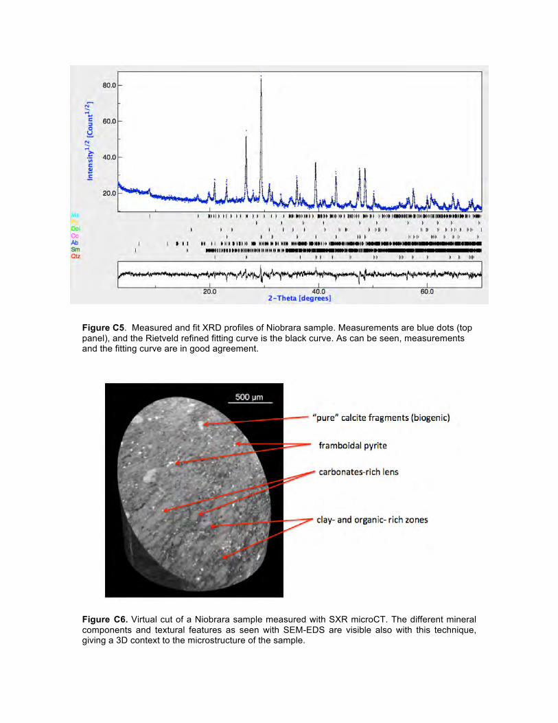
C2.2. X-Ray Powder Diffraction analysis To complete our initial characterization of the Niobrara shale sample, a fragment contiguous to the sample analyzed has been chosen and ground to a powder for XRPD analysis. The XRPD profile has been analyzed via Rietveld analysis to obtain quantitative information about the mineralogy of the sample. Results are as follows [weight%(sigma referred to the last digit)]: Quartz: 14.6(2) Smectite (~14Å): 6.6(4) Plagioclase: 3.5(3) Calcite: 48.5(3) Dolomite: 6.8(2) Pyrite: 2.1(1) Detrital mica - illite (modeled with a muscovite 2M1 structure): 17.5(4) Lattice preferred orientation was considered for phyllosilicates and carbonates. Turbostratic disorder for the smectite has been included in this analysis. As it is possible to see, the carbonates (mostly calcite) comprise slightly more than one half of the sample by weight. The crystallinity of the sampled calcite is not very high (meaning not as high as in sparry calcite), as it is possible to appreciate from the peak shape function and to indirectly infer from the sample preparation (top loading sample holder for XRPD) that did not induce appreciable crystallographic preferred orientation. This confirms the observation from the SEM where the calcite looks more micritic in nature.
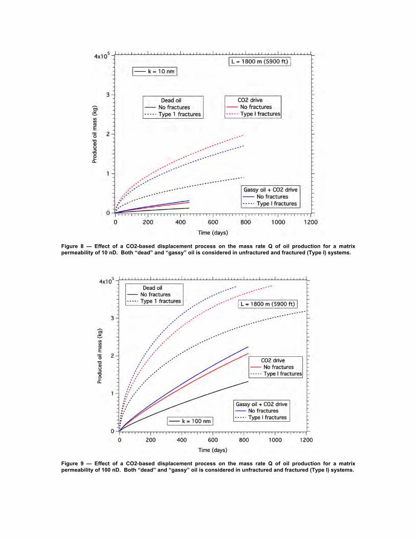
From this first characterization it is possible to see that this shale is very rich in carbonates (mostly calcite, with some dolomite), distributed in layers and in micrometric lenticular structures. The presence of the micritic calcite is also related to the microporosity of the sample. The clay amount is typical of many shales, with smectite (with significant structural/stacking disorder) and detrital mica, while other phyllosilicates such as chlorite and kaolinite seem to be absent. The organic-rich particles are scattered throughout the sample, and do not seem to follow the bedding by forming thin and flat structures like in many gas shales. Also, no significant porosity is visible at the magnification used for imaging. C2.3. Static x-ray Micro-CT Analysis To more thoroughly investigate the microstructure of the Niobrara shale, synchrotron x-ray (SXR) microCT was carried out on selected samples. This technique allowed us to obtain 3D data and study the sample in a perfectly undisturbed state (no need for vacuum or polished surface). The first observations obtained via SXR microCT confirm what seen using other imaging techniques: carbonates form lenticular structures surrounded by clay-rich layers a few µm thick. At a larger scale (~1mm) layering structures can be seen, highlighted by a different carbonates/clays ratio. Since the clay-rich layers are less attenuating, they are easily seen in SXR microCT datasets as darker layers (see Figures C5 and C6). The use of synchrotron radiation in this kind of analysis is advantageous since it is possible to take advantage of the monochromaticity and spatial coherence of the beam, and to choose proper compromises of resolution vs. field of view, to obtain very high-quality datasets. The facility used for these measurements is beamline 8.3.2. at the Advanced Light Source, at the LBNL.
Figure C5. Measured and fit XRD profiles of Niobrara sample. Measurements are blue dots (top panel), and the Rietveld refined fitting curve is the black curve. As can be seen, measurements and the fitting curve are in good agreement.
Figure C6. Virtual cut of a Niobrara sample measured with SXR microCT. The different mineral components and textural features as seen with SEM-EDS are visible also with this technique, giving a 3D context to the microstructure of the sample.
A preliminary investigation was also carried out to evaluate the potential of microCT for shale fracture imaging. A simple unconfined uniaxial breakage of samples was performed to see if the crack network generated could be related to textural features. In particular we wanted to see if the breakage of the sample would occur preferably in the clay-rich layers (Figure C7), a characteristic often encountered in shales (e.g., Mancos Shale). This preferential breakage can have an impact in the micro-fracturing behavior and also in the recovery of hydrocarbons, especially in case it would occur preferentially in hydrocarbon-rich layers. The geometry of the fracture surfaces is also important from a context of potential reactive surface area for a number of different processes. In this Niobrara sample we have not found any clear evidence that the breakage of the sample is strictly related to the clay-rich layers (Figure C7 to C9), even though evidence of some preferential splitting behavior has been observed.
Figure C7. Virtual thin section of the sample, where a better image of the bedding features is shown. It is possible to appreciate the compositional differences highlighted by the different attenuation of x-rays at different scales.
Figure C8. In this first experiment the fractures appeared irregular and seemed to be controlled primarily by applied stress state. They do not seem to be strictly related to the sample microstructure.
Figure C9. In this experiment the fractures look irregular as well, the main crack is has been generated at the interface of a clay-rich layer with a carbonates-rich layer, following the bedding plane. The clay-rich layer also shows a number of secondary fractures, while the carbonates-rich one is perfectly intact.
The material characterization via diffraction and electron imaging techniques, plus the starting, static, scans of the Niobrara shale samples, also provided an excellent starting point to plan the much more challenging dynamic SXR microCT experiments, aimed at understanding the behavior of oil shale at conditions compatible with hydrocarbon recovery processes in the reservoir. It is worth to remark that the combined effort of beam-line 8.3.2 at the ALS and the Earth Sciences Division of LBNL for real-time imaging of geochemical processes at reservoir conditions is a continuing effort. At the same time, the local x-ray imaging facility is a worldwide pioneering capability for dynamic imaging (4D XR microCT) and has amassed probably the most extensive experience on geological materials, as evidenced from the publication and presentation record. C.3. Laboratory Investigations: Fundamental Processes at the
Pore to Fracture Scale C3.1. Objectives The in situ SXR microCT experiments carried out were aimed at answering two questions: (1) How a fracture under a flow of carbonated water evolves. From a hydrocarbon
recovery point of view, this is a critical assessment, since if CO2 is used in the reservoir exploitation, and the reservoir rock is reactive at those conditions, significant modification of the microstructure and of the fracture geometry can occur. It is evident that if in the considered scenario the fractured behaves as self-sealing systems, the hydrocarbon recovery would be problematic. On the other hand, self-enhancing systems would increase the local permeability of the reservoir, thus potentially helping with the recovery of the product.
(2) The second question is related to EOR involves the utilization of liquid/supercritical CO2 as a solvent to sweep hydrocarbons from fractured oil shales. The efficiency and the repercussion on the fracture aperture and crack surface microstructure of this process at the pore scale are still poorly understood and our experiment tried to shed some light on this unknown.
C3.2. Experiment 1: Monitoring the development of the fracture during flow of carbonated water
In this first experiment we have prepared a 3/8” x 1” Niobrara shale core, cut in half vertically to simulate a fracture along the sample. Bedding plane was chosen to be sub-horizontal to highlight eventual features due to different layers composition. The experiment was carried out using the in-house developed triaxial cell able to perform in-situ measurement at the SXR-microCT beamline. The experimental conditions chosen for this experiment were:
o Pore pressure = ~1400 psi o Confining pressure = 1700 psi
o Fluid: equilibrated CO2-saturated water at 500 psi, ~25°C o Flow rate: 5 µl/min during the first part of the experiment, 10 µl/min during the
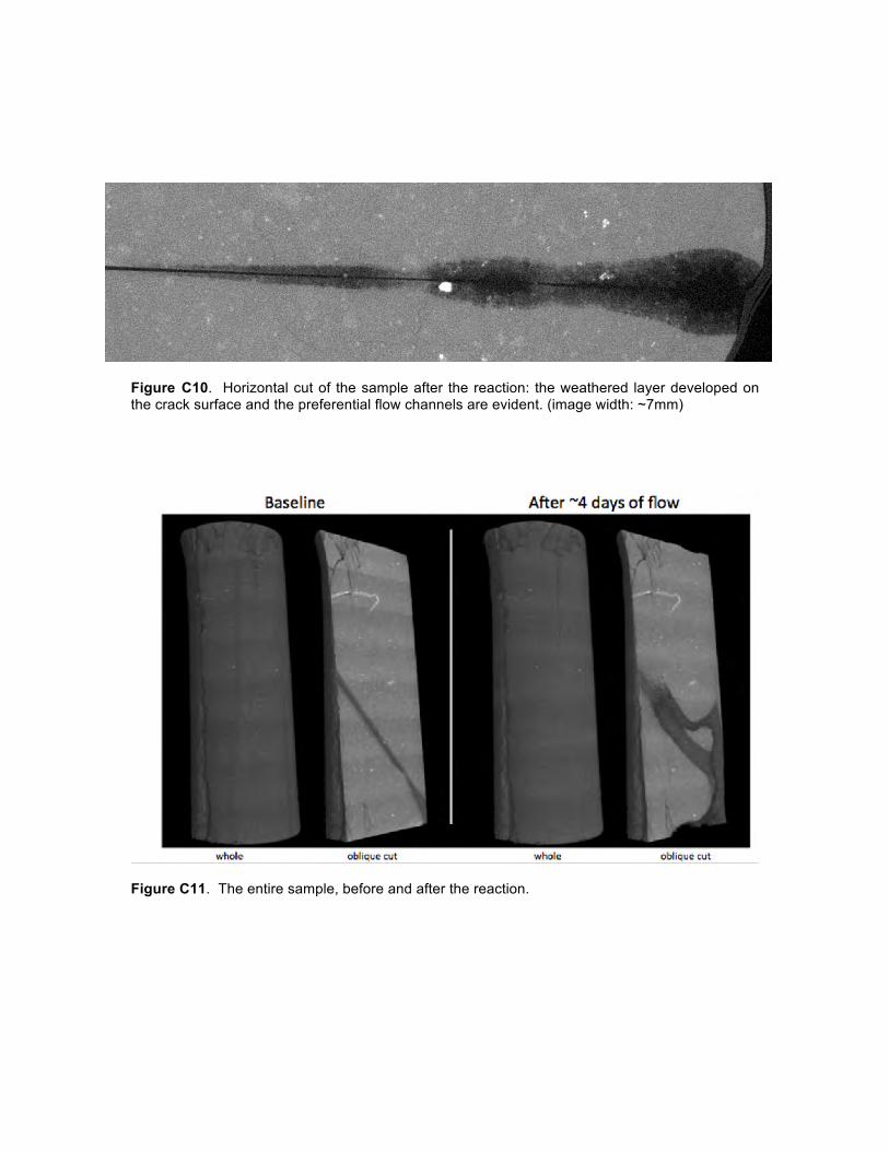
second part (to increase the extent of the reaction). Experimental Results The Niobrara shale showed some unexpected behavior. While the dissolution of the carbonates was relatively fast, as expected, the development of the surface of the fracture was different from any other rock investigated previously under similar conditions. Specifically, we observed the development of an unexpectedly wide weathered zone along the directions of preferential flow in the fracture, which was caused by the preferential dissolution of the carbonate-rich lenses (Figures C10 and C11). The resulting less soluble material on the fracture surface, mostly clays and quartz/feldspar, is not easily mobilized by the flow of the reactant, but resides on the fracture surface for at least a few hundred microns of thickness. The aperture maps (Figure C12) also show the development of the fracture geometry, with branching and the development of a “wormhole” structure with the evolution of the reaction. From the slice above it is possible to see that the microstructure of the crack surface is not smooth, but apparently it follows the texture of the rock. This is to be expected since the lens-shaped structures are expected to dissolve faster than any other component. The SEM study in Figure C13 also confirms this observation. From the SEM maps it possible to appreciate how the newly developed porosity is indeed due to the dissolution of the carbonate-rich lenses. A more interesting observation is that the residual clay-rich material is also enriched in organics (see C EDS map). To summarize the information pertinent to EOR obtained with this experiment, it is possible to affirm that, in this context (mini-core, limited reaction time): o There is an increase in permeability due to the worm-holing and preferential
dissolution of carbonate-rich structures. o Despite the development of a wide weathered zone along the preferential flow paths,
the dissolution does not generate a significant change in the contact points in the fracture (so the fracture is not closing under the applied confining pressure)
o The weathered zone is enriched in phases associated with the organic content of the rock, potentially making them more exposed in case techniques involving oil solvents were employed.
o The weathered zone, made for a significant part from clay flocs, is also likely to have weak mechanical properties (important in case proppants are considered: es. sand grains would embed very easily in this layer, losing their ability to keep the fracture open).
o The migration of fines is not significant, thus leading to the development of the extensive weathered zone on the crack surface.
Figure C10. Horizontal cut of the sample after the reaction: the weathered layer developed on the crack surface and the preferential flow channels are evident. (image width: ~7mm)
Figure C11. The entire sample, before and after the reaction.
Figure C12. Local thickness aperture maps of the fracture at different stages of the reaction. Each step covers the whole sample with an area approximately of 3/8”x1”. Inlet is at the bottom of the sample.
Figure C13. SEM analysis on one of the “branches” of the wormhole.
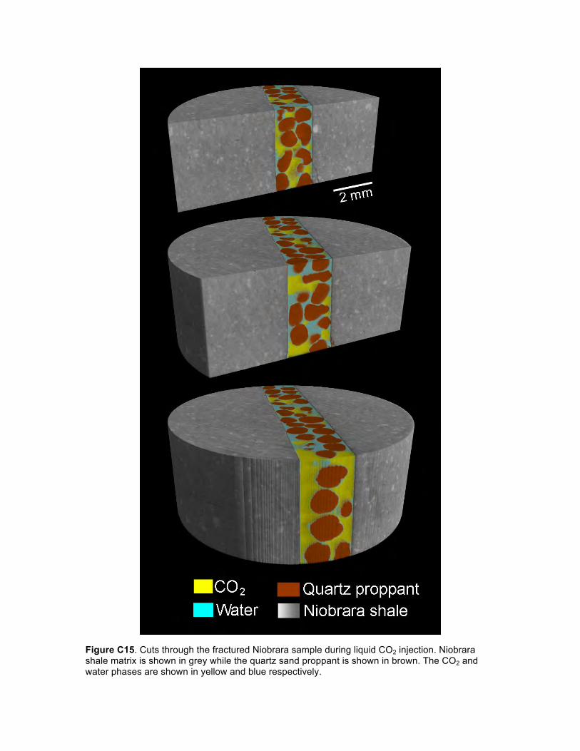
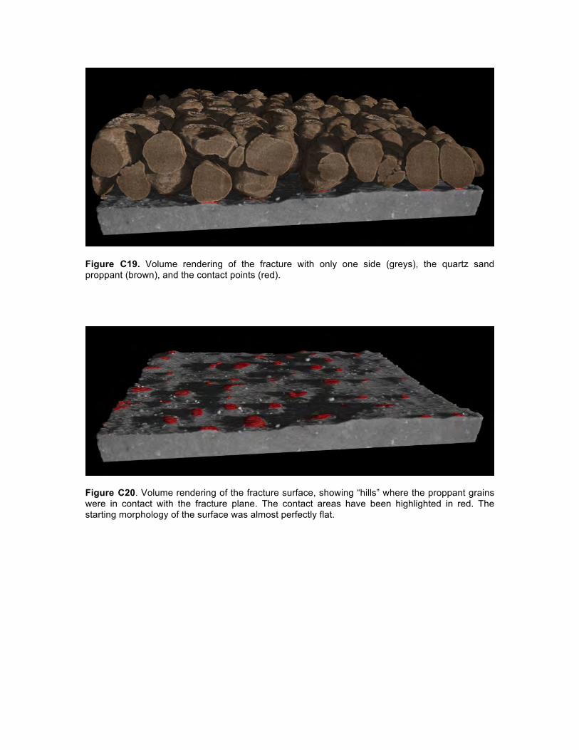
C3.3. Experiment 2: Effect of sweeping a propped fracture with liquid CO2 In this second experiment we attempted to study the behavior of a water-saturated sample of Niobrara shale, with a fracture filled with proppant. Main goal was to monitor the solvent action of liquid CO2 and eventual modifications to the fracture geometry, in particular proppant grain embedment in case of softening of the surface of the fracture. The experiment was again set using the triaxial cell shown in Figure C14. The sample was a Niobrara core ~ 3/8” (diameter) x 1/2” (height) in size, cut in half and filled with a double layer of sand grains (20/30 mesh). The sample was pressurized to a pore pressure of 1100 psi while confined at 1300 psi of hydrostatic stress. After this initial pressurization, a baseline microCT scan was acquired of the entire sample with an isotropic 6.87 µm voxel size. Pure CO2 was then compressed from gas to liquid phase (1100 psi, 24.6 °C) in an ISCO syringe pump and injected into the fractured sample at an initial rate of 100 µl/min for 3.25 hours followed by a first repeat scan. At this point flow was restarted at 25 µl/min for 11 hours followed by a second repeat scan. To the end of injection, approximately 36 mL of CO2 were injected through the fracture. After completion of the injection phase, another scan was taken increasing the confining pressure to 1700 psi, trying to induce fracture closure. Experimental Results The experiment showed extremely little change in the system. The first injection of liquid CO2 generated a partial displacement of the water in the sample, but a significant amount of water was left in the fracture, thus limiting the contact of the solvent (CO2(liq)) with the solvation target (the oil close to the fracture surface). Moreover, dissolution behavior, as described in the first experiment, is also limited, since a close to equilibrium state in the water with Ca++ and CO3
--/HCO3- ionic species is quickly reached, resulting in just a
limited amount of dissolution on the crack surface. This makes the whole system quite static, with exception of the two-phase flow: the solvation effect is limited by the pre-existing water, and at the same time the chemical reaction are significantly slowed down because of the fast saturation of the trapped water. Figure C15 shows a rendering of the sample after the injection. In a reactive system it would be expected to see some modifications on the crack surface (to better appreciate this pert of the sample a series of virtual cuts are presented), more specifically a decrease in the x-ray attenuation values (~decrease in density) at the surface of the crack, but this effect is virtually undetectable. In the renderings different components have been segmented and labeled with different colors for clarity. The “shale” component has been left in gray scale to better highlight its texture and the (non-)presence of eventual weathered zones on the crack surface. To better check for fine changes in the sample a further step in the analysis was taken. An equivalent vertical section of part of the sample was taken from the datasets before and after the reaction as can be seen in Figure C16. A registration procedure has been
employed to take into account the slight shifts of the sample due to mounting/ unmounting, compression, etc. A difference of the registered images has been calculated to highlight where changes in grayscale (~density) are present. In the figure below the vertical slices pre- and post- reaction are presented using a different lookup table to better highlight the differences (A and B). Apart from the zone with the fluids, the two images look close to identical. In panel C, the pre-reaction vertical section (in grays) with superimposed a colormap where a decrease in attenuation values occurred is plotted. This color map highlights where the reactions in the sample happened. It is evident that the extent of the reactions is extremely low and concentrated in some parts of the crack surface, apparently far from the proppant grains, where the flow and diffusion are likely to be faster, and in these zones the extent of the reaction barely reaches 20 µm in thickness.
Figure C14. New HP triaxial cell for reservoir sample imaging at Beamline 8.3.2. Panel A shows a close-up of the refurbished micro triaxial vessel during the experiment while panel B includes the beamline hardware including the optics frame (on the right).
Figure C15. Cuts through the fractured Niobrara sample during liquid CO2 injection. Niobrara shale matrix is shown in grey while the quartz sand proppant is shown in brown. The CO2 and water phases are shown in yellow and blue respectively.
Figure C16. Cross-sections of tomographic volume showing near-fracture region before (A) and after (B) liquid CO2 injection. Panel (C) shows the baseline image with color highlights in the narrow near-fracture regions which showed modification (only 2-3 voxels).
To summarize the results important from an oil recovery perspective obtained with this second experiment (we remark that the processes investigated with this experiment are limited to ~ one day): o The water in the sample cannot be effectively displaced. Therefore the effect of the
solvent, the CO2(liq), is strongly limited by the presence of the trapped water. This significantly limits the contact of the solvent with the oil close to the surface of the fracture.
o The trapped water and the two-phase flow also limits the transport of ionic species, thus creating a close to equilibrium situation in the water trapped at the contact with the crack surface, thus inhibiting the dissolution of the carbonates on the crack surface.
o Given the very limited modifications of the crack surface and the mechanical properties of the shale, in this experiment no variation of the fracture aperture is detectable when increasing confining pressure to 1700 psi (600 psi of differential pressure). The proppant is effectively keeping the fracture open.
C3.4. Experiment 3: Effect of sweeping a propped fracture with carbonated water
An experiment with similar conditions to the one presented above, but flowing carbonated water instead of liquid CO2 has been performed as well. The main goal for this experiment was to understand the role of the proppant in keeping the fracture open: more specifically, the aim was to check if the dissolution of the carbonates fraction of the rock would weaken the surface of the fracture enough (generation of a leached layer rich in clays, with poor mechanical properties) to embed the quartz grain and close the fracture progressively. Generation of the leached layer is of interest to enhanced production since it offers a path to modify the permeability of the near fracture region. The injection stage of the experiment was carried out outside the beamline, with similar parameters as the experiment utilizing liquid CO2: 1100 psi pore pressure, 1300 psi confining pressure, 35 ml of CO2-saturated water flown at 25 µl/min. After the injection stage, the equipment was moved at the beamline to execute the XR imaging part, and –after a first scan- to increase the confining pressure to increase the differential pressure trying to close the fracture. For this reason no baseline scan is available, but since the sample was cut, we can safely assume flat crack surfaces at the beginning of the experiment. From Figures C17 we can immediately appreciate the differences with respect the experiment involving liquid CO2, primarily the extent of the dissolution reaction within the fracture. As expected there is a significant amount of dissolution when using carbonated water, and the residual leached layer is still present, as for the experiment without the proppant. The higher flow-rate for this last experiment was also chosen to avoid wormholing and obtain a more uniform dissolution on the crack surface. As anticipated, wormholing in this experiment has not observed, but an interesting feature was observed instead: the proppant sand grains are efficiently protecting the surface of the fracture from dissolution at the contact points. This behavior highlights that the proppant is efficient in keeping the fracture open also via this mechanism, preventing dissolution of material at the important areas from a mechanical point of view, hinting at the fact that a very significant dissolution extent is needed before a first closure of the fracture might occur.
Figure C17. Volume rendering of a cutout of the sample, after injection. The weathered layer is clearly visible (dark grey) as are the sand grains and contact regions.
This behavior is further confirmed by the measurement done after increasing the confining pressure to a value of 750 psi of differential; the variation in the fracture aperture, with respect the first scan, is comparable in extent with the resolution of the measurement i.e. maximum a few microns. These last two experiments (Figures C18 to C20) highlight the behavior of a propped fracture at similar conditions using two different fluids for the injection. The effect on the fracture is very different, with almost no effect when sweeping with CO2(liq), while CO2(aq) is very efficient in modifying the surface morphology of the fracture. The only, extremely limited, effect observable when flowing CO2(liq) is due to the (slow) dissolution of CO2 in the trapped water, and once in solution the reaction with the carbonates can occur. This reaction is not only limited by the CO2 dissolution in the water, though, since the saturation in Ca2+ of the capillary-trapped fluid will also slow the reaction down very quickly. On the other hand, a steady supply of reactant and a prompt removal of cations from the dissolved minerals when flowing an aqueous solution of CO2 provides a fast dissolution of the carbonates, but the role of the proppant grains becomes important as well. The grains provide protection to the most important areas of the fracture from a mechanical point of view, inhibiting, at least at the initial stage, the closure of the fracture very efficiently. In a more practical scenario, when focusing on EOR strategies, it would be quite safe to assume that a propped fracture can undergo to a substantial amount of dissolution, when flown with CO2(aq) potentially increasing the permeability and exposing a clay-rich and organic-rich weathered layer on the fracture surface. On the other hand, the flow of CO2(liq) in a context of flowing a solvent to dissolve organics, would have only a limited impact on the microstructure of the fracture surface. We should note that a possible direction for further research would be water-alternating-gas (WAG) approaches with carbonated brines in the water phase. Whether or not the increase in porosity and
permeability in the near- fracture region enhances production remains an open question in these scenarios. These experiments can provide some hints, such as flowing first carbonated water to increase the permeability and expose organic-rich matter to the surface, then followed by liquid CO2 to dissolve the organics more efficiently, but more long-term process investigations (either with modeling or lab-scale experiments) would need to be considered to validate these observations from a strictly applied point of view.
Figure C18. Volume rendering of the sample, with an oblique virtual cut showing the main features. The microstructure of the weathered layer is similar to the one observed in the experiment with the fracture without proppant but here the dissolution is homogeneous. The exceptions are the proppant grain contact points, which efficiently protect the surface from the weathering process.
Figure C19. Volume rendering of the fracture with only one side (greys), the quartz sand proppant (brown), and the contact points (red).
Figure C20. Volume rendering of the fracture surface, showing “hills” where the proppant grains were in contact with the fracture plane. The contact areas have been highlighted in red. The starting morphology of the surface was almost perfectly flat.
APPENDIX D
Laboratory Investigations for Maximization of Production from Tight/Shale Oil Reservoirs: From Fundamental Studies to Technology
Development and Evaluation
Molecular Fluid Dynamics Studies
G. Waychunas Lawrence Berkeley National Laboratory
D1. Objectives Development of the capability for accurately modeling dissolved and clustered hydrocarbons interactions with both clay basal and edge sites within model clay pores, while observing the effects of flow on these molecular units. By using reactive potentials, MD can provide distinctive new information on surface-petroleum fluid interactions at physically observable scales. D2. Deliverables The most important overall result would be the modes of interaction of hydrocarbon molecules with pore surfaces. These include collection of molecules at particular pore sites, i.e. aggregation of molecules, breakdown of hydrocarbons at reactive clay sites, reorientation of molecules near pore surfaces and in higher flow fields, and overall molecular migration. Other results would include that nature of coverage and sorption of hydrocarbon molecules on clay pore surfaces, with attention to the expected differing behavior at clay basal planes (more hydrophobic) versus clay particles edges (largely hydrophilic). Another aspect to be determined are the effects of pressure and temperature on hydrocarbon aggregation and movement, and the P,T conditions that are optimal to allow hydrocarbon migration through tight pores. The work from this study may be extendable to more realistic dynamic simulations, such as larger clay particle aggregates (more complex pore structure), or to better realizations of flow effects, given more extensive computational ability. It should also be extendable to guide hydrocarbon-clay interfacial reaction calculations important in general biogeochemistry. Such reactions would include the breakup of hydrocarbon “clots”, solvation changes, vaporization into the accompanying gas phase, and others processes. These could be simulated with kinetic Monte Carlo approaches, perhaps buttressed with DFT (Density Functional Theory) energy calculations. Thus, the expected deliverables are: (1) Modes of interactions of hydrocarbon molecules with pore surfaces—collection and
concentration, breakdown, reorientation in flow, overall migration. (2) Sorption and coverage of clay surfaces (both relatively hydrophobic—basal planes, and
relatively hydrophilic—edge surfaces) by hydrocarbon molecules and clusterered hydrocarbons including molecules with substituted –COOH and –NH2 groups. This information could be reduced to thermodynamic and mechanical properties such as binding energies and wettability.
(3) Conditions (P,T etc) that have the largest effect on hydrocarbon migration and concentration. Contrawise, conditions that are the poorest for migration, or result in other problems in potential extraction (e.g. sequestration reactions).
(4) Base information extendable to more realistic simulations: larger simulation models with more complex pore structure, better realizations of flow effects
(5) Base information for hydrocarbon-clay interface reactions—likely done with DFT and KMC (Kinetic Monte Carlo) techniques (modeling reaction progress such as clot breakup, vaporization, solvation, etc.) as well as reactive MD combined with Umbrella sampling approaches (Yan and Yuan 2016).
D3. Molecular Fluid Dynamics Simulations D3.1. Clay Pore Interaction With Aqueous Solutions and Hydrocarbons A number of features of tight shale hydrocarbons are amenable to simulations, e.g. the phase relationship of vapor and fluid components (Makimura et al. 2013), the nature of interaction of fluids with clay mineral surfaces (Pitman and van Duin 2012), and the manner in which organic-containing fluids migrate through clay mineral assemblages (Kumar and Errington 2013). In this part of the LBNL effort we have focused on the latter two components, and have developed strategies for simulating them accurately and for systems of significant and relevant size. In order to model interactions with clay mineral surfaces we need to include both clay basal planes and clay mineral edges, the latter of which have seen sparse attention in past investigations, but whose importance has been well demonstrated (Liu et al 2014). However a parallel investigation at LBNL supported by DOE BES in our geochemistry program has allowed separate investigation of clay/mica edge structure and reactivity, and we have been able to leverage this improved understanding into the present work. The major differences between basal planes and edges are point of zero charge (PZC) and hydrophobicity. Basal planes are terminated by oxygens tied to silicon atoms, and are usually not very reactive, as their terminal proton is difficult to remove. This makes for a hydrophobic surface in general, which is somewhat mitigated if there is aluminum substitution for silicon creating net layer charge. Nevertheless, basal planes are thought to be unreactive with most organic components of natural fluids. Edge planes are terminated by oxygens tied to aluminum, silicon and magnesium. These oxygens are reactive if deprotonated, and can bind to certain functional groups of organic molecules. In our simulations we have thus included both types of clay mineral terminations, specifically by using a tunnel structure through a clay mineral crystal. By using such a model differential binding and local flow tendencies of aqueous and organic fluid components can be compared and contrasted. To be able to perform relevant simulations several conditions must be met. 1) the system must use aqueous or organic fluids which conform to known fluid and interactive properties. 2) the surfaces of the clay mineral phase must be realistically terminated and charged. 3) the size of the system must be large enough to probe flow interactions pat the nm regime (and ideally toward the micron regime), which still providing accurate information about local (atomistic) clay-fluid
interactions. Taken together, these requirements present difficulties for standard molecular dynamics (MD) simulations. For small systems (e.g. 100 atoms) it is possible to use ab initio MD (called AIMD or Car-Parinello MD) to determine the local minimum energy for parts of clay mineral surfaces, and for small volumes of fluids with reasonable computation time (Tazi et al 2012). Ab initio calculations allow for very good estimations of interaction parameters (potentials) between interacting atoms and molecules, and hence allow chemical reactions to be modeled, but cannot yet be scaled to the size regimes needed to study complex fluid interactions with mineral surfaces or pores. A way around this difficulty is to use classical MD simulations with so-called “reactive” potentials (van Duin et al. 2001). These interaction potentials are more complex than those used for standard classical MD, but can be implemented with much more efficiency than ab initio potentials (which must be recalculated very frequently during the simulation). Hence much larger systems can potentially be studied using reactive potentials with the drawback that their applicability may be less general than standard potentials which do not allow for chemical reactions to occur. Whereas standard MD potentials can be tested or “proofed” by comparing results with known information, such as fluid densities or pair correlation functions from x-ray scattering studies, the testing process for reactive potentials combines these tests with a subset of all possible reactions that the modeled system can undergo. In our case we begin with an aqueous fluid with dissolved organic molecules and wish to be able to follow deprotonation reactions of hydroxyls and carboxylic acid groups both in fluid and surface molecules, essentially adding acid-base reactivity to the system. Ultimately, reactive potentials that would allow more complex reactions, e.g. condensation, pyrolysis reactions and other organic processes would be needed to follow more extended fluid reactions. In our case, we began with a set of reactive potentials previously developed for silica-organic systems (Pitman and van Duin 2012) and extending it chemically by adding new interatomic potentials for use with clay mineralogy. Using this approach, we can readily extend simulations to 10,000 and more atoms, so that pores on the order of 5 nm can be explored. This allows the near surface interaction of fluid molecules and clay surfaces to be explored with computational times of days. Simulations of more than 1 million atoms would be possible with long machine time (months), affording pore sized of as much as 100 nm. Such simulations would allow complex flow interactions to be explored while building in the chemical reactivity. Other requirements of the simulation can be assessed by suitable testing in a non-reactive situation (fluid properties), while the termination of the clay mineral surfaces can be done by using the results of past ab initio calculations (Tazi et al 2012, Bickmore et al 2003) and knowledge of changes in local bonding due to expected surface charges and atomic substitutions (Tournassat et al 2003). For our purposes we also use separate energy calculations to relax the clay surfaces prior to the fluid-clay surface simulations. This overall approach is one of several that might be used for such clay-fluid systems. Others would include a mixed ab initio –mechanical modeling hybrid simulation where the fluid near the surface might be modeling with ab initio calculations, while the rest of the system is modeled using molecular modeling and/or standard MD potentials. We judged this type of approach to be fraught with more types of assumptions and tradeoffs than with a single type of reactive-potential
approach. We also felt that the development of a hybrid approach would not be possible within the time limits and personnel afforded by the initial phase of the project. D3.2. Adding Flow to Simulations There are many approaches to adding flow to MD-based simulations, among them external gravitational forcing fields, or resetting of molecular positions after a fixed number of time steps (OpenFOAM; Chen et al 2014; Cosden and Lukes 2013), effectively forcing a flow without adding system-wide gravitational force. Not all ways of adding flow velocity to a MD system have been evaluated for systematic prejudicing effects on simulation outcomes. This investigation evaluated these alternate approaches and tested their significance on relevant mineral-petroleum systems. The entire simulation approach is shown in Figure D1.
Figure D1. Flow chart for development of reactive potential MD. First an accurate pore (tunnel) model for a clay crystal is derived from known structure and existing ab initio calculations. This model is then tested for stability under MD. New potentials are generated to add appropriate atoms (e.g. K, Ca) and these are tested to check against proper water structure, etc. Then full model tested again for stable MD. Next hydrocarbon are added to the fluid and similar trials are done. This is the present state, whereby we are examining hydrocarbon interactions with surfaces. Next (future) step is adding flow to see changes in molecular interactions. A final goal is to link this scale of simulations to larger scale continuum (non-molecular) simulation models.
D4. Approaches and Results D4.1. Initial Approach To add in both chemical reactivity and flow effects to a MD aqueous hydrocarbon simulation in clay pores, used existing knowledge of shale fluid compositions rather than try to survey them from a separate set of Monte Carlo (GEMC) simulations. This is a required economy due to the limited resources (FTE time) available to the project. The reactive potentials now used (ReaxFF) were developed by the Van Duin group at PSU (van Duin et al 2001) and were implemented into the LAMMPS simulation package available at National Energy Research Supercomputer Center (NERSC) at LBNL. The potentials include those for H, C, O, Si, Al, and Cl. These constitute an improved set of potentials for RPMD, and they effectively cover the basic chemistry and expected reactivity of idealized clay pores (ReaxFF). As a first step, we added Fe to their potential set, and tested this using simple structural models (silica surfaces, oxide surfaces in equilibrium with water) to determine if Fe coordinations in solution and Fe-O distances were reasonable, and that use of the new potential set could yield appropriate pair distribution functions for bulk water. Slight changes in the Fe potentials were made to get best agreement with all observations. This then yielded a “hydrid” potential set with most reactivity intact, but extended to include Fe. Analogous work has been done to add Ca and Mg potentials. Further tests suggested that the set works well, and that the original reactive potential set could be extended in this way. The downside to this approach is that ideally all potentials should be recalibrated versus one another, a time-consuming task beyond the scope of the present project. Simulations of water pair-correlation parameters compared to those measured by Soper et al. (1997) by neutron diffraction are shown in Figure D2. Figure D3 is a movie of a water simulation over a slab of oxide.
Figure D2. O-O and O-H pair correlations derived from water using hybrid reactive potentials compared to the data from Soper. Both interatomic diatances and density yield good agreement.
Figure D3. Simulation movie of water at ambient conditions using hybrid reactive potentials and the LAMMPS code. The surface is a model oxide slab with three types of oxygen sites, approximating a clay mineral edge. The aqueous solution also contains dissolved silica. The oxygen is represented by red balls. Protons are shown in blue. For the new hybrid potential set, we obtained a very good agreement for Fe and K in solution, as well as for the water RDF parameters. The model includes about 4000 atoms.
Next a “hybrid” potential for K was obtained to extend the new potential set to practical clay compositions. At this time this larger set is still being tested, with the use of a new structural model closely incorporating what we understand about clay surfaces and edges. The next phase of the study allowed us to set up non-flow simulations for muscovite or illite clay compositions with a range of aqueous hydrocarbon fluids, and kaolinite and annite could also be simulated. In order to proceed to the next step in the flow chart for this work (Figure D1), the results of these non-flow tests must be consistent with known experimental results for interface structure, solid-hydrocarbon and solid-water interactions. If there is disagreement the hybrid potentials may need to be adjusted to best-fit experimental results. At this point we began exploratory runs of a series of simulations to examine the predicted reactivity of hydrocarbon molecules with clay surfaces. This uses the improved physical clay pore model shown in Figure D4 with more than 10,000 atoms. The runs examined aggregation at pore irregularities (such as the intersection of two grain surfaces), examine chemical breakdown at edge sites, examine possible hydrocarbon molecule injection into the clay interlayer, and test for catalyzed hydrocarbon reactions. The scope of the simulations was adjusted as we proceed to optimize a direction toward the project objectives. Thorough evaluation of the static simulations is required before moving to a dynamic flow system. D4.2. Reactive Potential Simulations D4.2.1. Water structure at clay surfaces Water structure near edge planes vs. basal planes of montmorillonite and muscovite (Figure D4) is different out to about 6 Å. The basal plane is roughly the same in both, but there are considerable differences between the types of edges, and also with changes in the degree of protonation of the edges. We have been using the edge protonation model of Bickmore et al. (2003), and the basal plane protonation model from various theoretical and experimental works. D4.2.2. Binding of carboxylic acids and alkanes on edge planes Pentanoic carboxylic acid binds differentially toward edges and basal planes. It forms more inner sphere complexes on the former, as well as several types of outer sphere complexes on both. Longer simulations, including umbrella sampling would be needed in any future work to get a better handle on these types of surface interactions, and the most stable surface configurations. The results of this study are discussed in the caption of Figure D5. D4.2.3. Binding of pentanoic acid and alkane on clay basal Here, carboxylic acid forms outer sphere complexes on the protonated basal surface, while pentane forms only aggregations away from the surface (although enough simulations have not been done to define what “aggregations” mean as of this point).. The results of this study are discussed in the caption of Figure D6. D4.2.4. Binding of carboxylates acid and alkanes to surfaces The results (Figure D7) appear to indicate that carboxylates tie alkanes to surfaces. Although we cannot yet state how general this result is, it seems likely that the relative proportions of alkanes and substituted alkanes (esters, acids, etc.) in an aqueous mixture will affect the way that all are bound to surfaces. This should be of major consequences in very fine pores within shales when
Figure D4. Muscovite “tunnel” (clay pore model) built to accurately model edge and basal plane sites and correct substitutional chemistry. Approximately 10,000 atoms are involved, including water in the pore itself. The internal surfaces are optimized for best agreement with existing edge models and both bond-valence and DFT calculations. (Red: oxygen; large purple: potassium; light blue: aluminum; dark blue: silicon; light brown: hydrogen). The basal plane substituting atoms (top of tunnel) can be varied to change layer charge. Edge sites (sides of tunnel) are created after existing ab initio models and ongoing DOE-BES research probing mica/clay edge site structure. Protonation of all surfaces is determined from known pka values and from ab initio calculations (ref). These can be varied further to reflect conditions such as with EOR procedures (more acidic etc). Fluid placed into the tunnel comprises about 5,000 atoms for a total simulation block of 15,000 atoms.
Figure D5. Top: Carboxylic acid (O2C-) sorption on montmorillonite edges. Inner sphere (centered about 0.4 Å from the “nominal” surface), outer sphere (about 2.6 Å from the surface) and Stern layer (about 5 Å from the surface) complexation appears to occur. Here we show average positions of observed simulated complexes. Sharper peaks refer to the structure of the clay near the surface including potassium, aluminum, magnesium, silicon and oxygen atoms. Changes in surface protonation affect these types of complexes and their relative proportions, but more simulations are needed to define these dependences. Bottom: Compare carboxylate sorbed situation with this plot of pentane “sorption”. The alkane is located in a wide distribution well above the surface, about 5.5-6Å. Essentially this is a hydrophobic interaction, and is observed for the most protonated edge conditions. Alkane complexation, or segregation, appears more localized to basal planes or to clusters in the aqueous fluid than near edges.
0
0.5
1
1.5
2
2.5
3
-4 -2 0 2 4 6
Montmorillonite edge -COOH sorption
Atom
ic d
ensit
y
Distance from surface (Å)
K
Al, Mg
S i, O
O, O2C-
O2C -
0
0.5
1
1.5
2
2.5
3
-4 -2 0 2 4 6 8 10
Monmorillonite edge plane C5H
12
Atom
ic d
ensit
y
Position relative to surface (Å)
Figure D6. Plots of pentanoic acid (left) and pentane (right) in aqueous solution near the montmorillonite basal planes. As in other plots water is not shown, and contributiosn are depicyed as Gaussians of width indicating spread of species and height indicating density. The carboxylic acid forms only outer sphere complexes and likely unbound complexes, while the pentane appears to form aggregates near the surface but not closely bound. Hence the relationship of both organics contrasts sharply with results from the edge planes.
Figure D7. Mixed pentanoic acid and pentane appear to behave quite differently from the individual agents. The left plot shows pentane near the monmorillonite edge plane and it is basically unbonded. However in the right hand plot the pentane is much closely attached by way of intervening inner sphere and outer sphere pentanoic acid groups. This suggests that the hydrophilic part of the carboxylic acid can influence the near surface geometry of alkanes.
0
0.2
0.4
0.6
0.8
1
1.2
-4 -2 0 2 4 6 8 10
Montmorillonite basal plane C5O
2H
10
Atom
ic de
nsity
Position relative to surface (Å)
Si
OO
C5O
2H
12 outer sphere C
5O
2H
12 unbound
0
0.2
0.4
0.6
0.8
1
1.2
-4 -2 0 2 4 6 8 10
Montmorillonite basal plane C5H
1 2
Atom
ic
dens
ity
Position relative to surface (Å)
0
0.5
1
1.5
2
2.5
3
-4 -2 0 2 4 6 8 10
Monmorillonite edge plane C5H
12
Atom
ic d
ensit
y
Position relative to surface (Å)
0
0.5
1
1.5
2
2.5
3
-4 -2 0 2 4 6 8 10
Montmorillonite edge C5O
2H
10 + C
5H
12
Atom
ic de
nsity
Position relative to surface (Å)
the fluid has significant water content. For fluids with minor water content, it is unclear what the extent of protonation of edge planes would be, and thus the interactions are not yet predictable. An extension of the work here to fluids with minor water is necessary. D4.3. Summary We have completed the bulk of the work needed to utilize reactive potentials in MD simulations of aqueous fluids containing organic components in porous clay media. The new potentials appear to adequately model water structure and ion solvation, though additional testing is required prior to publishing. Such potentials and the reactive potential approach replace the need for ab initio modeling to follow surface chemical reactions, and hence allow for useful reactive simulations of large systems. In our case this has been up to 15,000 molecules, but it is possible to extend the work to approximately 106 molecules, thus being close to the near sub micron scale. The model structures that have been generated appear to be good representations of monmorillonite (and muscovite) structure including basal and edge planes, and their near-atomic structure and protonation state. Simulations have been conducted with water, water plus alkanes, water plus carboxylic acids, and water plus both species. Significant differences have been observed in the nature of the surface interactions (both edge and basal plane) with both species separately, and there is significant interaction at the surfaces when the species are mixed. In particular carboxylic acids appear to help bind alkanes to the edge surfaces. We expect that similar effects might be due with substituted alkanes, such as from carboxylic, amino, hydroxyl and other functional groups have some hydrophilic character. Hence alkane simulations alone appear to be insufficient to accurately model surface interactions. D5. Continuation of the Study and Future Work Flow studies done with two different strategies to move the fluid in the clay tunnels were planned for this study, but have not yet been performed. This would be an important, and indeed critical, part of future work. We expect large molecules to be affected topologically by flow conditions, e.g., by orienting themselves in the flow stream, and so the combinations of varied surface interactions and flow conditions must be explored to understand near surface fluid transfer. Other needed work includes simulations on other alkanes and substituted alkanes to determine if the results here are general, or specific to our particular simulation model or simulation geometry. For example, how would a narrow tunnel affect interactions? A tunnel with surface irregularities such as large atomic steps? With flow simulations we need to determine what flow rates are associated with changes in local surface interactions, i.e. if there is a regime where there is decoupling of near surface bound species and others further from the surface. Finally, we expect variations in fluid behavior as the organic-aqueous ratio changes in the fluid, reflecting the different hydrophobic-hydrophilic character of the fluid components and the different clay
mineral surfaces. Hence a range of fluid compositions, particularly those indicative of actual tight shale EOR conditions, needs to be investigated. D6. Leveraging Aspects (1) With generous support from DOE in terms of a computation-simulation summer student funded by the DOE CSGF program, we were able to take the first steps in working with and developing hybrid clay reactive potentials concurrent with the present project, saving considerable effort and time. (2) Collaborative work using existing classical MD potentials (Clayff) has been initiated with the clay simulations group at LANL (Cygan and Greathouse, e.g. see Zeitler et al., 2014). This will be a continuing effort that encompasses parts of an ongoing DOE-BES project centered on mica edge reactivity (GW focus). This collaboration lends strength particularly to the testing part of the existing NETL work, as well as considerable expertise in MD simulations using the LAMMPS codes (Plimpton, 1995). (3) The DOE-BES project at LBNL-ESD will yield new information on clay edge structure that is not presently available. This will allow clay pore simulation models to be more accurate. D7. DOE Facilities Usage The NERSC systems (the EDISON and HOPPER supercomputers) have been used for the needs of this project. Some clay/mica surface/edge work is being done at SSRL and APS involving DOE-BES leveraging research that will be useful for this project (e.g. composition and structure of clay particle edges). D8. References Bickmore et al. (2003) Ab Initio determination of edge surface structures for dioctahedral 2:1
phyllosilicates: Implications for acid-base reactivity. Clays Clay Minerals 51:359 Chen et al. (2014) OpenFOAM for computational fluid dynamics. Notices of the AMS 61:354 Cheng et al (2001) Molecular-scale density oscillations in water adjacent to a mica surface. Phys.
Rev Lett 87:156103 Cosden and Lukes (2013) A hybrid atomistic-continuum model for fluid flow using LAMMPS
and OpenFOAM. Comp Phys Comm 184:1958 Deneke et al (2003) Grazing incidence (GI) XAFS measurements of Hf(IV) and U(VI) sorption
onto mica surfaces. PCCP 5:939 Gu and Evans (2007) Modelling the adsorption of Cd(II), Cu(II), Ni(II), Pb(II), and Zn(II) onto
Fithian Illite. J Coll Interface Sci 307:317 Ilton et al (2004) Heterogeneous reduction of uranyl by micas: Crystal chemical and solution
controls. Geochim Cosmochim Acta 68:2417 Kumar and Errington (2013) Understanding wetting of immiscible liquids near a solid surface
using molecular simulation. J Chem Physics 139: 064110
Kunieda et al (2010) Self-accumulation of aromatics at the oil-water interface through weak hydrogen bonding. J Amer Chem Soc 132: 18281
Liu et al (2013) Activity of edge surface sites of montmorillonite and kaolinite. Geochim. Cosmochim Acta 117:180
Liu et al (2014) Surface force measurements at kaolinite edge surfaces using atomic force microscopy. J Coll Interface Sci 420:35
Lorenz et al (2008) Molecular dynamics of ion transport and electrokinetics effects in realistic silica channels. J Phys. Chem 112:10222
Makimura et al (2013) Application of molecular simulations to CO2-ehnanced oil recovery: Phase equilibria and Interfacial phenomena. SPE Journal April 2013: 319
Neumann et al (2013) Spectroscopic evidence for Fe(II)-Fe(III) electron transfer at clay mineral edge and basal sites. Environ Sci Technol 47:6969
Pitman and van Duin (2012) Dynamics of confined reactive water in smectite clay-zeolite composites. J Amer Chem. Soc. 134:3042
Steinhauer and Ganzenmuller (2011) The implementation of smooth particle hydrodynamics in LAMMPS. SPH-User documentation.
Tazi et al (2012) Absolute acidity at clay edge sites from ab-initio simulations. Geochim Cosmochim Acta 94:1
Tournassat et al (2003) nanomorphology of montmorillonite particles: Estimation of the clay edge sorption site density by low-pressure gas adsorption and AFM observations. Am Mineral 88:1989
Van Duin et al. (2001) ReaxFF: A reactive force field for hydrocarbons. J. Phys. Chem A 105:9396
Yan et al (2011) Determination of anisotropic surface characteristics of different phyllosilicates by direct force measurements. Langmuir 27:12996
Yan et al (2013) Interaction of divalent cations with basal planes and edge surfaces of phyllosilicate minerals: Muscovite and talc. J Coll Interface Sci 404:183
Yan and Yuan (2016) Molecular Dynamics simulation of of the oil detachment process within silica nanopores. J Phys Chem C 120:2667
Zeitler et al (2014) Vibrational analysis of brucite surfaces and the development of an improved force field for molecular simulation of interfaces. J Phys Chem C 118:7946
Zhau et al (2008) Probing charge potentials of clay basal planes and edges by direct force measurements. Langmuir 24:12899