Numerical Conformal Mappings for Regions Bounded by - DiVA

c© by Anders Andersson. All rights reserved.

Anders Andersson

Numerical ConformalMappings for RegionsBounded by SmoothCurves

Licentiate Thesis

Växjö University

Department of Mathematics and Systems Engineering

Reports from MSI



Numerical Conformal Mappings for Regions Bounded by Smooth

Curves



Anders Andersson

Numerical Conformal Mappings for

Regions Bounded by Smooth Curves

Licentiate Thesis

Mathematics

Växjö University


A thesis for the Degree of Licentiate of Philosophy in Mathematics at Växjö University.

Numerical Conformal Mappings for Regions Bounded by Smooth Curves

Anders Andersson

Växjö University

Department of Mathematics and Systems Engineering

se- Växjö, Sweden

http://www.vxu.se/msi


Reports from MSI, no.

issn -

isrn vxu-msi-ma-r----se


Abstract

In many applications, conformal mappings are used to transform two-dimensional regions into simpler ones. One such region for which conformalmappings are needed is a channel bounded by continuously differentiablecurves. In the applications that have motivated this work, it is impor-tant that the region an approximate conformal mapping produces, hasthis property, but also that the direction of the curve can be controlled,especially in the ends of the channel.

This thesis treats three different methods for numerically constructingconformal mappings between the upper half–plane or unit circle and a re-gion bounded by a continuously differentiable curve, where the directionof the curve in a number of control points is controlled, exact or approxi-mately.

The first method is built on an idea by Peter Henrici, where a modifiedSchwarz–Christoffel mapping maps the upper half–plane conformally on apolygon with rounded corners. His idea is used in an algorithm by whichmappings for arbitrary regions, bounded by smooth curves are constructed.

The second method uses the fact that a Schwarz–Christoffel map-ping from the upper half–plane or unit circle to a polygon maps a region Qinside the half–plane or circle, for example a circle with radius less than 1or a sector in the half–plane, on a region Ω inside the polygon bounded bya smooth curve. Given such a region Ω, we develop methods to find a suit-able outer polygon and corresponding Schwarz–Christoffel mapping thatgives a mapping from Q to Ω.

Both these methods use the concept of tangent polygons to numericallydetermine the coefficients in the mappings.

Finally, we use one of Don Marshall’s zipper algorithms to constructconformal mappings from the upper half–plane to channels bounded by ar-bitrary smooth curves, with the additional property that they are parallelstraight lines when approaching infinity.

Key-words: Schwarz–Christoffel mapping, rounded corners, tangent poly-gons, outer polygon, zipper algorithm.

v


Sammanfattning

Inom många tillämpningar används konforma avbildningar för att trans-formera tvådimensionella områden till områden med enklare utseende. Ettexempel på ett sådant område är en kanal av varierande tjocklek begränsadav en kontinuerligt deriverbar kurva. I de tillämpningar som har motiveratdetta arbete, är det viktigt att dessa egenskaper bevaras i det område enapproximativ konform avbildning producerar, men det är också viktigtatt begränsningskurvans riktning kan kontrolleras, särkilt i kanalens bådaändar.

Denna avhandling behandlar tre olika metoder för att numeriskt kon-struera konforma avbildningar mellan ett enkelt standardområde, före-trädesvis det övre halvplanet eller enhetscirkeln, och ett område begränsatav en kontinuerligt deriverbar kurva, där begränsningskurvans riktning kankontrolleras, exakt eller approximativt.

Den första metoden är en utveckling av en idé, först beskriven av Pe-ter Henrici, där en modifierad Schwarz–Christoffel–avbildning avbildar detövre halvplanet konformt på en polygon med rundade hörn. Med utgångs-punkt i denna idé skapas en algoritm för att konstruera avbildningar pågodtyckliga områden med släta randkurvor.

Den andra metoden bygger också den på Schwarz–Christoffel–avbild-ningen, och utnyttjar det faktum att om enhetscirkeln eller halvplanetavbildas på en polygon kommer ett område Q i det inre av dessa, somtill exempel en cirkel med centrum i origo och radie mindre än 1, ellerett område i övre halvplanet begränsat av två strålar, att avbildas på ettområde R i det inre av polygonen begränsat av en slät kurva. Vi utvecklaren metod för att hitta ett polygonalt område P , utanför det Ω som manönskar att skapa en avbildning för, sådant att den Schwarz–Christoffel–avbildning som avbildar enhetscirkeln eller halvplanet på P , avbildar Qpå Ω.

I båda dessa fall används tangentpolygoner för att numeriskt bestämmaden önskade avbildningen.

Slutligen beskrivs en metod där en av Don Marshalls så kallade zipper-algoritmer används för att skapa en avbildning mellan det övre halvplanetoch en godtycklig kanal, begränsad av släta kurvor, som i båda ändar går

vi


mot oändligheten som räta parallella linjer.

Nyckelord: Schwarz–Christoffelavbildningen, rundade hörn, tangentpo-lygoner, yttre polygoner, zipper–algoritmer.

vii


Acknowledgments

First, I wish to express my warmest gratitude to my supervisor Prof. BörjeNilsson, for all the support I have achieved from the first time we met, longbefore I officially became his doctoral student. Even though involved inmany activities and with a crowded schedule, he seems to always have timefor a discussion, and he shows no annoyance over a silly question. Manyimportant ideas in this thesis originate from him. A lot of fruitful andencouraging discussions have also taken place with my assistant supervisorJoachim Toft, for which I thank him.

A very special thanks goes to my friend and colleague Tomas Biro.He worked hard to get me in contact with the Växjö University and theresearch team he belonged to, and without all his initiatives and encour-agement during many years, I would never have restarted any doctoralstudies.

I also thank my employer in Jönköping, the School of Engineering,that most generously has supported me in this project. My gratitudegoes also to my friends and colleagues at the Department of Mathematicsand Physics at the School of Engineering, especially Tjavdar Ivanov andFredrik Abrahamsson, for many fruitful discussions and good advice.

Last but not least, I thank my wife Lena and my children. Withouttheir support and love, it had not been possible to finish or even to starta project like this.

viii


Contents

Abstract v

Sammanfattning vi

Acknowledgments viii

1 Introduction 1

2 The Schwarz–Christoffel Mapping 5

3 Tangent Polygons 11

4 The Rounded Corners Method 16

4.1 A modified Schwarz–Christoffel mapping . . . . . . . . . . 16

4.2 Constructing the conformal mapping . . . . . . . . . . . . . 18

4.3 Conclusions and Comments . . . . . . . . . . . . . . . . . . 26

4.4 Examples . . . . . . . . . . . . . . . . . . . . . . . . . . . . 27

5 The Outer Polygon Method 35

5.1 Finding the Outer Polygon . . . . . . . . . . . . . . . . . . 36

5.2 The Existence of an Outer Polygon . . . . . . . . . . . . . . 38

5.3 Example . . . . . . . . . . . . . . . . . . . . . . . . . . . . . 40

5.4 Comments . . . . . . . . . . . . . . . . . . . . . . . . . . . . 44

6 The Zipper Method 45

6.1 The Zipper algorithms . . . . . . . . . . . . . . . . . . . . . 45

6.2 Constructing the Mapping Function . . . . . . . . . . . . . 47

6.3 Examples . . . . . . . . . . . . . . . . . . . . . . . . . . . . 50

ix


Contents

7 Summary and Conclusions 57

7.1 Suggestions for future work . . . . . . . . . . . . . . . . . . 58

x


Chapter 1

Introduction

Conformal mappings have for more than 100 years, been important toolsin engineering, mathematical physics and mathematics. For example, theuse of a conformal map to transform the boundary in a two-dimensionalboundary value problem, can often be an important part of the solutionof the problem.

Which method shall then be used to construct a suitable conformalmapping? Suppose that we have a model region Ω, and are trying to finda function that maps a simple region R (half-plane, unit circle, horizontalstrip) conformally on Ω. The Riemann mapping theorem states that sucha mapping exists. And there are many methods available for constructingconformal maps numerically, [8] and [12], together with [19] and [16] lista wide collection of numerical methods. And each method produces amapping function, which, more or less accurately, approximates one of thepossible functions that the Riemann mapping theorem deal with for R andΩ. Suppose that such an approximate function f maps R on a region Φ.This region Φ may have some of the properties that characterize Ω, butmay lack others or may just have them approximately. Normally, it iscertain properties of the boundary ∂Ω that are in focus of our attention.Of course, we expect any method to be able to produce a mapping thatmakes the boundary ∂Φ pass close to at least a finite number of pointsin ∂Ω. But does the mapping we choose give ∂Φ the same direction that∂Ω has in points where the boundaries coincide? And what about infiniteregions? Which mappings can give ∂Φ some characteristic properties that∂Ω has, all the way to and through infinity?

One potential application for conformal mappings is the modelling ofwave scattering in two-dimensional and some three-dimensional curvedwaveguides with a varying cross section [13]. The first step in this proce-

1


Chapter 1. Introduction

dure consists of cutting the infinite two-dimensional waveguide into finitelength pieces transformed into infinite sub-waveguides by adding inlet andoutlet with constant width. With the so-called building block method[14, 3], the scattering properties of the original waveguide will be synthe-sized from the corresponding properties of the sub-waveguides. Secondly,each sub-waveguide is mapped conformally to a horizontal strip resultingin a scattering problem for which an efficient and stable numerical methodexists. This wave scattering method is based on that the model regionhas parallel walls. Furthermore, the mapping is a numerically tractableproblem due to the confinement of the varying part to a finite part of themodel region.

So, if we generalize, given a region Ω, we want to construct a mappingfunction that conformally maps a simple region R on a region Φ, where werequire that ∂Φ has the same direction as ∂Ω in some set of control points.Especially, in the case ∂Ω passes infinity as a straight line, it is necessarythat ∂Φ does so, and that the two curves have the same direction throughinfinity. Of course, we also want ∂Φ to be a good point-wise approximationof ∂Ω. Therefore, ∂Φ must have a high degree of regularity between thecontrol points. If ∂Ω changes direction monotonously, ∂Φ should do thesame, and if ∂Ω is smooth, ∂Φ should be smooth.

Before we continue, we shall make a small remark concerning the ter-minology: When we talk about smooth boundary curves, here as well as inthe title and the rest of the thesis, we mean curves that changes directioncontinuously, i.e. at least one time (but not necessarily more) continuouslydifferentiable curves.

Concerning the smoothness, several methods exist. In fact, most ex-isting numerical methods result in functions between one of the simpleregions and regions with a smooth boundary curve. We can use one of thepolynomial approximations or different integral equation methods, pre-sented in [8, 12, 19, 16]. If the region Ω can be mapped on a region that isnearly circular, we can use this property to find an approximate function.Ken Stephenson’s circle packing method [17] would be another alternativeto consider. Most of them result in regions bounded by smooth curves,but neither of these methods give the required control over the directionof the boundary curve.

When focusing on the direction, it is natural to think of the Schwarz-

2


Christoffel mapping [7] from a simple region to a polygon. The very heartof this function is that the polygon sides have exactly the direction wedecide, even if the polygon vertices are just approximately determined.But to achieve smoothness, we need to use some modified form of thismapping.

And there are as a matter of fact some generalizations of the Schwarz-Christoffel mapping available, mappings that could give smooth boundarycurves. In 1979, Davis [4] published a method, where he constructs map-pings where one or several of the polygon sides are not straight lines butpolynomial curves. We also have the method developed by Bjørstad andGrosse [2] and later Howell [11], were mappings for regions bounded bystraight lines and circular arcs are developed.

A major break-through for practical use of the Schwarz-Christoffelmapping was when Trefethen made public his pioneering methods [18],including the use of compound Gauss-Jacobi quadrature for calculatingthe integrals. This work has later been extended by himself, by Driscoll[7], Howell [10] and others. It has also been made accessible for a greaterpublic in the user-friendly Schwarz-Christoffel toolbox for Matlab [6], madeby Driscoll.

In this work, we use three different methods for constructing conformalmappings for regions bounded by smooth curves. The first method usesan idea by Peter Henrici [9], where a modified Schwarz–Christoffel map-ping maps the upper half–plane conformally on a polygon with roundedcorners. This idea is used to construct mappings for arbitrary regions,bounded by smooth curves.

The second method uses the fact that a Schwarz–Christoffel map-ping from the upper half–plane or unit circle to a polygon maps a regionQ inside the half–plane or circle, for example a circle with radius less than1 or a sector in the half–plane, on a region R inside the polygon boundedby a smooth curve. Given such a region R, we try to find a suitableouter polygon and corresponding Schwarz–Christoffel mapping that givesa mapping from Q to R.

The concept of tangent polygons together with the Fréchet distancegives a useful measure for the boundary curves the approximated functionsproduce, and is in both the above methods used as a tool for the numericdetermination of the coefficients in the mappings.

3


Chapter 1. Introduction

Finally, we present a method where we use one of Don Marshall’sZipper algorithms. The Zipper algorithm [5] by Don Marshall is a veryfast and accurate method for numerical conformal mappings. One of itsvariants, the geodesic algorithm, generates a smooth boundary curve, andis here used to construct a conformal mapping from the upper half–planeto a channel, bounded by two arbitrary smooth curves, curves that areparallel straight lines when approaching infinity.

A short description of the Schwarz–Christoffel mapping is given inchapter 2. Tangent polygons and related topics are presented in chapter3. Chapters 4, 5 and 6 contains the three methods, and in chapter 7, thereis a short discussion concerning their advantages and drawbacks.

4


Chapter 2

The Schwarz–Christoffel Mapping

The Schwarz–Christoffel mapping

z = f(w) = A

∫ w

w0

n∏

k=1

(ω − wk)αk−1dω +B, (2.1)

maps the upper half-plane conformally and one to one, onto a polygonwith interior angles α1π, . . . , αnπ. The real numbers w1, . . . , wn are calledprevertices, and are preimages under f of the polygon’s vertices z1, . . . , zn.Infinite zk:s are allowed. Infinity is by f mapped on a point on the polygonside znz1. It is possible to omit the last factor (ω − wn)αn−1 in (2.1), inwhich case infinity is mapped on the last polygon vertex zn.

Of course, finding suitable constants A,B,w0, . . . , wn in (2.1) is nottrivial. It is clear that |A| resizes, argA rotates, and that B together withw0 translates the polygon. But the placing of the prevertices w1, . . . , wn

rules the polygon’s side-lengths in a non-obvious and non-linear way. Westate that this so called parameter problem always has a solution.

Theorem 2.1. Given a polygon P with vertices z1, . . . , zn, we can findreal constants w1, . . . , wn and complex constants A and B, such that (2.1)is a conformal mapping from the upper half-plane to P .

Proof. The proof follows Henrici [9]. According to the Riemann mappingtheorem, there is a function g which conformally maps the upper half–plane Imw > 0 to the interior of P . The Osgood–Carathéodory theoremensures that g is a continuous and one-to-one mapping from Imw ≥ 0 toP . Let for k = 1, . . . n the preimage of zk be wk, and suppose that ∞ ismapped to z0. We may also suppose that w1 < w2 < · · · < wn.

Let Λk be the line segment between wk and wk+1. Since g maps Λk

on a straight line segment, g can, by the Schwarz reflection principle, becontinued analytically across Λk into the lower half–plane.

5


Chapter 2. The Schwarz–Christoffel Mapping

g is a conformal mapping, hence g′(w) 6= 0 for Imw > 0, and wecan define the function G(w) = log g′(w) which is analytic for Imw > 0.But since a region containing Λk between wk and wk+1 is by g mappedone-to-one onto a region containing the straight line zkzk+1, g

′(w) 6= 0in this region, and since arg g′(w) is constant and hence ImG′(w) = 0on Λk, G

′(w) can likewise be extended analytically across Λk. The sameargument holds for every k, and it follows that G′(w) can be extended toan analytic function in the whole plane with the possible exception of thepoints w1, . . . , wn on the real axis.

For any k, define

h(w) =(

g(w) − zk

)1/αk .

Clearly, h(wk) = 0, and in a neighbourhood of wk, h is analytic if Imw > 0and continuous and one-to-one for Imw ≥ 0. If arg(w−wk) increases from0 to π, arg(g(w)−zk) increases by αkπ, and arg h(w) by π. Hence, h mapsthe straight line segment [wk−ε, wk +ε] on a straight line segment through0. Then, even h can be extended by the Schwarz reflection principle to aconformal mapping of the disk |w − wk| < ε.

Hence, h can be expanded in power series about wk, i.e.

h(w) = c1(w − wk) + c2(w − wk)2 + . . . ,

and therefore,

g(w) = zk + c∗1(w − wk)αk(

1 + c∗2(w − wk) + . . .)

from which it follows that

G′(w) =g′′(w)

g′(w)=

αk − 1

w − wk+ analytic function.

The above can be done for each of the singularities wk, and hence, thefunction

Φ(w) = G′(w) −n∑

k=1

αk − 1

w − wk

6


is entire. If z0 is the image of infinity under g and α0π the inner angleat z0, (α0 = 1 if the polygon has no vertex at z0), we can by similarcomputations as above find that

g

(

1

w

)

= z0 + c∗1wα0(1 + c∗2w + . . . ),

near w = 0, and hence for |w| sufficiently large

g(w) = z0 + c∗1w−α0(1 + c∗1w

−1 + . . . ).

Thus,

G′(w) =g′′(w)

g′(w)=

−α0 − 1

w+O(w−2)

when w → ∞, from which follows that

limw→∞

Φ(w) = 0,

and hence by Liouville’s theorem, Φ(w) is entirely zero. Hence, for somecomplex constant A,

G(w) = log g′(w) = log

(

A

n∏

k=1

(w − wk)αk−1

)

,

from which the theorem follows.

We have in the proof assumed a finite polygon, but with a similarargument, one can show that the theorem holds even for polygonal regionswith one or several vertices infinite.

During recent years, very efficient numerical methods for solving theparameter problem have been developed. We have in this work used theSC-toolbox [6] by Trefethen and Driscoll, and it constructs a Schwarz–-Christoffel map with w1 = −1, wn−1 = 1 and wn = ∞. If necessary, theMoebius transformation

m(w) =w − 1

w + 3(2.2)

takes us between this version of (2.1), and a version with all the preverticesfinite.

7



Many variants of the Schwarz–Christoffel mapping have been devel-oped. If the polygon is finite, a good alternative is to make a mappingfrom the unit circle to the polygon, which result in a formula very similarto (2.1). If the polygon is a channel, i.e. a polygon with two of its ver-tices in infinity, it seems natural to start with for example the horizontalchannel w = x + yi, x ∈ R, 0 ≤ y ≤ 1, and develop a correspondingSchwarz–Christoffel mapping. All this and much more is implemented inthe toolbox [6].

However, in most of the applications in this work, we use mappingsfrom the upper half–plane. For a polygonal channel with parallel walls atthe ends, a Schwarz–Christoffel mapping from the upper half–plane to thepolygon takes the form

s(w) = A

∫ w

w0

(ω − a)−1n−2∏

k=1

(ω − wk)αk−1 dω +B. (2.3)

Here, w1, . . . , wn−2 are real preimages of the finite vertices z1, . . . , zn−2

and a is a point on the real axis, mapped to infinity at one of the channelends. The other infinite channel end is the image of ∞. We note thatthe rays from a in the upper half–plane is mapped on curves which at thechannel ends tend to be parallel to the channel walls. This fact is statedmore precise in the following theorem:

Theorem 2.2. Assume that in the mapping s, given in (2.3), from theupper half–plane to a polygonal channel with parallel walls at the ends,

−∞ < w1 < w2 < · · · < wm < a < wm+1 < · · · < wn−2 <∞.

Then, the image of any ray w = a + reiϕ from a in the upper half–planehas asymptotes

s(a+ r) +Aiϕ, r ∈]1 − a,∞[, when r → ∞ (2.4)

and

s(a+ r) +Aiϕn−2∏

k=1

(a− wk)αk−1, r ∈]0, a− wm[, when r → 0. (2.5)

8


Furthermore, the set of curves s(a + reiϕ) : 0 < ϕ < π converges uni-formly with respect to ϕ to their asymptotes both when r → ∞ and whenr → 0.

Proof. With the change of variable ω = a+ reit, the integral

∫ a+reiϕ

a+r

∏n−2k=1(ω − wk)

αk−1

ω − adω = i

∫ ϕ

0

n−2∏

k=1

(a− wk + reit)αk−1 dt,

and hence,

s(a+ reiϕ) − s(a+ r) = Ai

∫ ϕ

0

∏

k

(a− wk + reit)αk−1dt.

Clearly, for any ε > 0, there is R0 > 0 such that if 0 < r < R0,∣

∣

∣

∣

∣

s(a+ reiϕ) − s(a+ r) −Aiϕ∏

k

(a− wk)αk−1

∣

∣

∣

∣

∣

< ε

for all ϕ ∈ [0, π]. Further, since the channel walls are parallel at the ends,

n−2∑

k=1

(αk − 1) = 0,

which means that

Ai

∫ ϕ

0

∏

k

(a− wk + reit)αk−1dt−Aiϕ =

Ai

∫ ϕ

0

[

∏

k

(

1 +a− wk

re−it

)αk−1

− 1

]

dt,

and hence, for any ε > 0, we can find R such that if r > R,

∣

∣s(a+ reiϕ) − s(a+ r) −Aiϕ∣

∣ ≤

|A|∫ ϕ

0

∣

∣

∣

∣

∣

∏

k

(

1 +a− wk

re−it

)αk−1

− 1

∣

∣

∣

∣

∣

dt < ε

for all ϕ ∈ [0, π].

9



For a Schwarz–Christoffel mapping from the upper half–plane as it isgiven in (2.1), argA is the direction of the polygon side between zn andz1, or, if the polygon is a channel with parallel walls at the ends and themapping given as in (2.3), argA is the direction of the channel at the endwhich is the image of infinity. From the preceding theorem, it also followsthat |A| can be determined from the channel width at that end.

Corollary. The distance d between the two parallel walls in a polygonalchannel at the end that is the image of infinity is given by

d = π |A| . (2.6)

Proof. Follows from (2.4) with ϕ = π, in which case the asymptote coin-cides with the polygon side.

10


Chapter 3

Tangent Polygons

In our work we consider smooth curves, enclosing simple regions, which inthe case they pass infinity, do so as straight lines. From such curves, weconstruct polygons by taking tangents to the curves in a suitable set ofpoints. This motivates the following definitions:

Definition 3.1. A tangent point on a curve Γ in the complex plane is apair (z, ϕ), where z is a point on the curve and ϕ is the angular directionof the curve in that point.

Definition 3.2. A ctp (curve with tangent points) is a curve Γ, enclosinga simple region, with the following properties:

1. Γ is smooth, in the meaning that it changes direction continuouslyeverywhere but at infinity. This means that Γ is one time (but notnecessarily many times) continuously differentiable.

2. There is a real constant K such that any parts of Γ lying outside thecircle |z| ≤ K are straight lines.

3. On Γ, there is a finite set MΓ = (zk, ϕk)|k = 1, . . . , n of tangentpoints. The tangent points are numbered such that (zk+1, ϕk+1)comes after (zk, ϕk) when following the curve in anti-clockwise di-rection. We can use (zn+1, ϕn+1) as a synonym for (z1, ϕ1). Further,the directions ϕk are given such that 0 < |ϕk+1 − ϕk| ≤ π. The setof tangent points is chosen such that

(a) ϕk+1 6= ϕk.

(b) If Γ contains only finite points between zk and zk+1, then|ϕk+1 − ϕk| < π.

11


Chapter 3. Tangent Polygons

(c) There is at least one tangent point on each straight line part ofΓ.

(d) Any point of inflexion on a non-linear part of Γ is in MΓ.

Property 2 means that if Γ passes infinity, it does so as a straightline. From 3(a) and (c) follows that there is exactly one tangent point oneach straight line part of Γ. 3(d) ensures that the direction of Γ changesmonotonously between the tangent points.

Theorem 3.1. To each ctp, there is a unique polygon PΓ having sides thatare tangents to Γ through the tangent points.

Proof. The tangents are determined by the tangent points. Outside thecircle |z| ≤ K, we see from property 2 and 3(c) that Γ coincides withits tangents. If Γ does not pass infinity between the subsequent tangentpoints zk and zk+1, by properties 1 and 3(a),(b) the point of intersectionbetween the tangents

zk + |zk+1 − zk|sin(

ϕk+1 − arg(zk+1 − zk))

sin(ϕk+1 − ϕk)eiϕk , (3.1)

is a finite point in the complex plane. Hence each pair of subsequenttangent points generates a unique polygon vertex.

Note that the polygon is not necessarily simple, it might intersect itself.However, in this work, we consider ctp:s with simple polygons, somethingthat can always be achieved by taking sufficiently many tangent points onthe curve.

Definition 3.3. Two ctp:s Γ1 with MΓ1= (zk, ϕk) and Γ2 with MΓ2

=(wk, ψk) are said to be d-uniform if |MΓ1

| = |MΓ2| = n, and if for all

k = 1, . . . , n

ϕk = ψk and |zk − wk| ≤ d. (3.2)

Since the directions are equal, d-uniform ctp:s pass infinity betweencorresponding tangent points.

To measure the distance between two curves in the complex plane, weuse the Fréchet distance [1][15].

12


zk

zk+1

z′k

Figure 3.1: Getting a vertex z′k by intersecting the tangents in zk and zk+1

Definition 3.4. Let Γ1 and Γ2 be two curves in the complex plane. Thenthe distance

δ(Γ1,Γ2) = infα,β

maxt∈[0,1]

|α(t) − β(t)|, (3.3)

where α and β ranges over all possible parametrisations [0, 1] → Γ1 and[0, 1] → Γ2 respectively.

We note that δ is a metric on the family of all piece-wise smooth curvesin the complex plane, and that δ(Γ1,Γ2), δ(PΓ1

, PΓ2) and δ(Γ1, PΓ2

) existand are all finite if Γ1 and Γ2 are d-uniform.

Two polygons are said to be parallel if they have the same number ofvertices (of which some could be infinite) and if corresponding sides in thepolygons are parallel.

Theorem 3.2. Let Γ1 and Γ2 be d-uniform ctp:s with MΓ1= (zk, ϕk)

and MΓ2= (wk, ϕk), and let F be the set of all k ∈ 1, . . . , n such that

13


Chapter 3. Tangent Polygons

Γ1 is finite between zk and zk+1. Then

δ(Γ1,Γ2) ≤ maxk∈F

|zk+1−zk|2 sin

|ϕk+1−ϕk|2 + d

cos|ϕk+1−ϕk|

2

. (3.4)

Proof. We consider first the case where d = 0, i.e., MΓ1= MΓ2

. Clearly,the Fréchet distance between these curves equals the maximum of the dis-tance between the curves between subsequent tangent points. If the curvespasses infinity between zk and zk+1, they coincide between those tangentpoints, so we may consider only the finite parts of the curves. Let forany k ∈ F , z′k be the point of intersection between the tangents throughzk and zk+1. Since the direction of the curves changes monotonously be-tween zk and zk+1 but no other restriction on the curvature is given, thecurves could be anywhere inside the triangle zkz

′kzk+1. Hence, the dis-

tance between the curves is less than the distance from z′k to the segmentzkzk+1. With given angle at z′k, this distance is greatest when the triangleis isosceles. The height in an isosceles triangle with base |zk+1 − zk| andπ − (ϕk+1 − ϕk) as interior top angle is

|zk+1 − zk|2

tanϕk+1 − ϕk

2,

and since Γ1 and Γ2 are ε-uniform, δ(Γ1,Γ2) exists, and it follows that forε = 0,

δ(Γ1,Γ2) ≤ δ(Γ1, PΓ1) ≤ max

k∈F

|zk+1 − zk|2

tan|ϕk+1 − ϕk|

2

. (3.5)

For d > 0, PΓ1and PΓ2

are parallel polygons where the distancesbetween parallel sides are less than or equal to d. These polygons haveinterior angle π−(ϕk+1−ϕk) at vertex k, and the Fréchet distance betweenthem is less than or equal to the greatest distance between correspondingvertices, i.e.,

δ(PΓ1, PΓ2

) ≤ d

cos(

ϕk+1−ϕk

2

) . (3.6)

For the distance between Γ1 and Γ2, we have

δ(Γ1,Γ2) < δ(Γ1, PΓ2),

14


and the triangle inequality for the Fréchet distance gives

δ(Γ1, PΓ2) ≤ δ(Γ1, PΓ1

) + δ(PΓ1, PΓ2

),

from which the theorem follows.

15


Chapter 4

The Rounded Corners Method

4.1 A modified Schwarz–Christoffel mapping

Rounding the corners in a Schwarz–Christoffel mapping

Henrici [9] has described a method to round the corners in a polygon,by modifying the related Schwarz–Christoffel mapping. We use a slightlymodified variant of this method.

Theorem 4.1. Let f be a Schwarz–Christoffel mapping that maps the up-per half-plane onto a polygon P with vertices z1, . . . , zn and correspondingpre-images w1, . . . , wn. Let all pre-images of finite vertices be finite. If thefactors

sk(ω) = (ω − wk)αk−1, k = 1, . . . , n (4.1)

are replaced by

hk(ω) =

ak

(

(ω − (wk − εk))αk−1 + (ω − (wk + εk))

αk−1), αk > 1

bk(

(ω − wk + εk)αk − (ω − wk − εk)

αk)

αk < 1

(4.2)where wk − εk > wk−1 + εk+1, we get a mapping function g with thefollowing properties:

(i) g maps the upper half-plane conformally and one-to-one onto a regionQ.

(ii) In the intervals [wk − εk, wk + εk], arg g′(w), the direction of theboundary curve g(w) changes continuously and monotonously. Out-side the intervals [wk−εk, wk+εk], the curves f(w) and g(w), w ∈ R,have the same direction. This means that Q is a “polygon” withrounded corners.

16


4.1. A modified Schwarz–Christoffel mapping

(iii) The tangent polygon Pg(R) differs from P in both size and shape.However, with ak = 1/2 and bk = 1/2αkεk,

limω→∞

hk(ω)

sk(ω)= 1.

Proof. (i) and (ii) are proved in [9]. For (iii), we note that for |ω − wk| >εk, we have

(ω − wk ± εk)γ

(ω − wk)γ=

(

1 ± εk

ω − wk

)γ

=

(

1 +∞∑

n=1

(±1)n γ(γ − 1) . . . (γ − n+ 1)

n!

(

εk

ω − wk

)n)

.

This means that

1

2

(

(ω − wk + εk)αk−1 + (ω − wk − εk)

αk−1)

=

(ω − wk)αk−1

(

1 +∞∑

n=1

(αk − 1) . . . (αk − 2n)

(2n)!

(

εk

ω − wk

)2n)

(4.3)

and

1

2αkεk((ω − wk + εk)

αk − (ω − wk − εk)αk) =

(ω − wk)αk−1

(

1 +∞∑

n=1

(αk − 1) . . . (αk − 2n)

(2n+ 1)!

(

εk

ω − wk

)2n)

, (4.4)

from which (iii) follows.

It is evident from the theorem that one cannot just replace the factorsin the Schwarz–Christoffel mapping , and as a result, get a polygon thatapart from the rounded corners has the same size and shape. By choosingthe constants a and b as in (iii), the sizes of the polygon and its roundedcousin are approximately the same, but as is seen from (4.3) and (4.4),we have an extra real factor in the integral for each rounded corner. And

17


Chapter 4. The Rounded Corners Method

this factor is not constant; it varies with the distance from the roundedcorner where it has its origin. This affects the side-lengths and thereforethe shape of the rounded polygon. Note also that these effects are biggerwhen α is far from 1, i.e. when there is a sharp angle at the roundedcorner.

Another side effect from the roundings is shown if we look at the dis-tance across the rounded corners. It might also be changed, as is illustratedby the integrals

Isk=

∫ wk+εk

wk−εk

sk(ω) dω =εαk

k (1 − eiπαk)

αk, (4.5)

and

Ihk=

∫ wk+εk

wk−εk

hk(ω) dω =

(2εk)αk(1 − eiπαk)

αk(αk + 1), αk < 1

2αk−1εαk

k (1 − eiπαk)

αk, αk > 1

. (4.6)

If we want to use roundings of corners to construct a certain mapping,one must take these side effects into account. In the case of at most onefinite polygon side, all the effects described here are easily handled byadjusting the multiplicative constant A, but with more than two finitevertices we must make further changes in the mapping to get a polygon ofa requested size and shape.

4.2 Constructing the conformal mapping

Constructing a modified Schwarz–Christoffel mapping

Let D be a simply connected region in the complex z-plane, bounded bya smooth curve Γ. To make Γ a ctp, we choose a set of tangent points(z1, ϕ1), . . . , (zn, ϕn) on it, fulfilling the requirements in property 3 for actp. Then the tangent intersections z′1, . . . , z

′n are determined by letting

z′k = ∞ if Γ is infinite between zk and zk+1, and according to (3.1) oth-erwise. z′1, . . . , z

′n are vertices in the polygon PΓ, and with any existing

18


4.2. Constructing the conformal mapping

software for Schwarz–Christoffel mappings , one can find a function

f∗(w) = A∗

∫ w

w0

n∏

k=1

(ω − w′k)

αk−1dω +B∗, (4.7)

that maps the upper half-plane onto the polygon PΓ.Now, the method described in Section 4.1 can be used to round the

corners. To each finite vertex z′k in the constructed polygon with corre-sponding pre-vertex wk, an εk is assigned. Then make a new function f(w)where each factor corresponding to finite z′k and wk in f∗ is replaced sothat

f(w) = A

∫ w

w0

n−1∏

k=1

hk(ω)dω +B, (4.8)

where according to Section 4.1

hk(ω) =

1

2αkεk

(

(ω − wk + εk)αk − (ω − wk − εk)

αk)

, αk < 1

1

2

(

(ω − wk + εk)αk−1 + (ω − wk − εk)

αk−1)

, αk > 1

. (4.9)

The sizes of the εk:s must be taken into some consideration. To make surethat at least one point on each polygon side is unaffected by the roundings,i.e., has the direction ϕk of the curve in the tangent point (zk, ϕk), we canfor all k choose

0 < εk < min(wk − wk−1, wk+1 − wk)/2. (4.10)

However, as is described later, smaller values of εk can be necessary.In the previous section, we saw that the rounding of corners changes

the shape of the polygon. However, with small εk:s and many tangentpoints, we can get a good approximation of a given region.

Theorem 4.2. Assume that the continuously differentiable curve Γ is theboundary of a simple connected region Ω. Then, by rounding the cornersin a Schwarz–Christoffel mapping for a tangent polygon, it is possible toconstruct a function that maps the upper half-plane conformally on a re-gion with a boundary curve C, that is also continuously differentiable andarbitrarily close to Γ.

19



Proof. Put tangent points on Γ, and let f∗ and f be the functions definedin (4.7) and (4.8), a Schwarz–Christoffel map for the tangent polygon PΓ

and its modified variant with rounded corners. Let sk be a factor in f∗,hk be the corresponding modified factor, and let finally C be the curvef(w) : w ∈ R. It follows now from (4.3) and (4.4) together with thedominated convergence theorem, that for the straight line parts of C,

limε→0

∣

∣

∣

∣

∣

∣

∫ wk+1−εk+1

wk+εk

∏

j

hj(ω) −∏

j

sj(ω)

dω

∣

∣

∣

∣

∣

∣

= 0. (4.11)

For the curved parts, we first note that

∏

j

hj −∏

j

sj = (hk − sk)∏

j 6=k

hj + sk

∏

j 6=k

hj −∏

j 6=k

sj

.

In the interval I = [wk − εk, wk + εk], and for any small positive εj , thefactors hj and sj are bounded for j 6= k, so let for some small r > 0

M1 = sup0<εj<r

j 6=k

maxw∈I

∣

∣

∣

∣

∣

∣

∏

j 6=k

hj(w)

∣

∣

∣

∣

∣

∣

and

M2 = sup0<εj<r

j 6=k

maxw∈I

∣

∣

∣

∣

∣

∣

∏

j 6=k

hj(w) −∏

j 6=k

sj(w)

∣

∣

∣

∣

∣

∣

.

Then, from (4.5) and (4.6) and since∣

∣1 − eiπαk∣

∣ ≤ 2, we have

∣

∣

∣

∣

∣

∣

∫ wk+εk

wk−εk

∏

j

hj(ω) −∏

j

sj(ω)

dω

∣

∣

∣

∣

∣

∣

≤

M1

∣

∣

∣

∣

∫ wk+εk

wk−εk

(hk(ω) − sk(ω)) dω

∣

∣

∣

∣

+M2

∣

∣

∣

∣

∫ wk+εk

wk−εk

sk(ω) dω

∣

∣

∣

∣

≤

2εαk

k

αk(cM1 +M2), (4.12)

20



where c = 1−2αk−1 if the rounded corner is concave, and c = 1−2αk/(αk+1) otherwise.

By assuming tangent points on the straight line parts of C as close toΓ:s tangent points as possible, the two curves are d-uniform ctp:s, and if(zk, ϕk) is the set of tangent points on Γ, it follows from Theorem 3.2,that the distance between Γ and C is

δ(Γ, C) ≤ maxk

|zk+1−zk|2 sin

|ϕk+1−ϕk|2 + d

cos|ϕk+1−ϕk|

2

,

where d originates from (4.11) and (4.12) and depends on the εk:s. SinceΓ is continuously differentiable, we can, by taking many tangent points,make all the |zk+1 − zk| and |ϕk+1 − ϕk| arbitrarily small. And by takingsufficiently small εk:s, d can also be made arbitrarily small. This provesthe theorem.

However, using the technique suggested by Theorem 4.2 to get a goodapproximation, would in most practical cases, due to the many tangentpoints needed, result in a complicated mapping function. There might becrowding problems [18, 7, 10], and the calculation of function values bynumerical integration of a product with maybe hundreds of fairly compli-cated factors, is time consuming and errors derived from the calculationsmay also enter in the results. We therefore do not recommend this “manytangent points and small ε:s”-technique for practical use.

Resolving the parameter problem

In the cases that have motivated us, we have found the rounding of cornersmethod useful with much fewer tangent points. Also, most curves coincidemuch more with the curve we construct, than what is indicated by Theorem3.2. The distance given there is in fact the distance between the tangentpolygon and a polygon with the tangent points as vertices, and both theconstructed curve and many model curves are quite far from both theseextremes. But to handle the side effects from the roundings when we usefewer tangent points, we have to resolve the so called parameter problem,i.e., re-determine the constants A,B,w1, . . . , wn in f .

21



Determining the parameters To do this redetermination with for ex-ample Newton’s method, we must formulate a set of equations. In an ordi-nary Schwarz–Christoffel mapping , we know that f∗(wk) in (4.7) shouldbe equal to some known vertex in the polygon, and from that, equationsto solve the parameter problem can easily be written down. When thecorners are rounded, the situation is more complicated. The images of thewk:s are points on the curve, situated somewhere in the roundings of thecorners, and the pre-images of the tangents points zk are not known inadvance.

Instead, we observe that the curve that is the image of the real axiscan be turned into a ctp with tangent points that have the same directionsas the tangent points on Γ.

Let C be the image of the real axis under f , and equip C with thetangent points (ζ1, ϕ1), . . . , (ζn, ϕn), where

ζk =

f(w1 − 2ε1) k = 1

f(

wk+wk+1

2

)

k = 2, . . . , n− 1

f(wn−1 + 2εn−1) k = n

, (4.13)

and construct its tangent polygon with vertices ζ1, . . . , ζn. Observe that ifwe choose the εk:s small enough, C for all k really has the direction ϕk inthe point ζk, since ζk is the image of a point on the real axis outside theinterval [wk − εk, wk + εk].

We can now compare side-lengths in the polygons PΓ and PC , deter-mined from Γ and C. Each of the polygons has n vertices, and hence wecan formulate n − 2 equations. If the n vertices are all finite, two of then side-lengths in the polygons are dependent on the others together withthe given directions. If the polygons has one vertex at infinity, we stillhave n− 2 comparable finite side-lengths. And finally, if the polygons arechannels, i.e., polygons with two infinite vertices , there is a total of n− 3finite side-lengths in the two parts of the polygon. In our work, we haveconsidered channels with parallel ends, and there the distance between thetwo parts at one of the ends gives the failing equation.

Let for k = 2, . . . , n− 1 Lk,C = |ζk − ζk−1|, i.e., the length of side k inPC , and let Lk,Γ be the corresponding side-length in PΓ. By elementary

22



trigonometry we see that

Lk,C =|ζk − ζk−1| sin(arg(ζk − ζk−1) − ϕk−1)

sin(ϕk − ϕk−1)+

|ζk+1 − ζk| sin(arg(ζk+1 − ζk) − ϕk)

sin(ϕk+1 − ϕk). (4.14)

The side-lengths Lk,Γ in PΓ are evaluated similarly.Now,

Lk,C = Lk,Γ, k = 2, . . . , n− 1 (4.15)

is a system of n−2 non-linear equations. Just like in an ordinary Schwarz–Christoffel mapping, three of the parameters can be set in advance.

We have used the half-plane map function in SC-toolbox [6] on thepolygon PΓ to get initial values for w1, . . . , wn and A. The toolbox putsw1 = −1, wn−1 = 1 and wn = ∞. If all vertices are finite, we use (2.2) toget a mapping with w1 = −1, wn−1 = 0 and wn = 1. Keeping these, weare using our n−2 equations (4.15) to re-determine w2, . . . , wn−2 and |A|.

Note that only the absolute value of the complex constant A has tobe re-determined. The argument of A, which rotates the polygon, shouldof course be left unchanged when applying Henrici’s corner roundings.Indeed, since the integrands in (4.7) and (4.8) are real for w > wn−1+εn−1,the argument of A equals the direction of the last polygon side, i.e., thedirection ϕn of the last tangent point. This means that the n−2 unknownsare all real numbers, as well as the left- and right-hand sides in the n− 2equations. Further, in the case of a channel with parallel walls at the endsas in Example 4.4, |A| can be determined analytically. It follows from thecalculations in the proof of Theorem 2.2 together with (4.3) and (4.4) thatthe distance between the channel walls at the end that is the image ofinfinity is |A|π.

The system (4.15) can be solved using numerical methods. We haveused Newton’s method with the parameters in the Schwarz–Christoffel mapf∗ as a starting approximation.

Existence of parameters Can the parameters A,w1, . . . , wn be foundfor any reasonable choice of ε1, . . . , εn such that the equations (4.15) hasa solution? Or geometrically: Does there for any ctp exist a polygon with

23



corners rounded by the method described here, such that its straight linesides coincides with the tangents to the ctp in the tangent points?

Theorem 4.3. Let

w1 < w2 < · · · < wn, A

be parameters in a Schwarz–Christoffel function g, mapping the upper half-plane on a polygon. Keeping w1, wn−1, wn and argA constant, define w =(w2, . . . , wn−2, |A|), and let

S(w) = (|g(w2) − g(w1)| , |g(w3) − g(w2)| , . . . , |g(wn−1) − g(wn−2)|)

be a vector containing n − 2 of the polygon sides. Let further w∗ be thesolution of the Schwarz–Christoffel parameter problem for the tangent poly-gon PΓ to a ctp Γ, i.e. S(w∗) contains n − 2 of the polygon sides in PΓ,and let ε = (ε1, . . . , εn), where εk ≥ 0.

If the Jacobian∂S

∂w(w∗) 6= 0,

then there exist a d > 0, such that if |ε| < d, a solution wε of the parameterproblem can always be found, when g is modified using ε to round thecorners.

Proof. Let

F (w, ε) = (L2,C , . . . , Ln−1,C) − (L2,Γ, . . . , Ln−1,Γ), εk ≥ 0,

where Lk,C and Lk,Γ are defined as in (4.14). Then we have F (w∗, 0) = 0and by defining F (w, ε1, . . . , εk, . . . , εn) = −F (w, ε1, . . . ,−εk, . . . , εn) ifεk < 0, we can extend the definition of F to comprise negative εk:s. F isdifferentiable with respect to w in a neighbourhood of (w∗, 0) and

∂F

∂w(w∗, 0) =

∂S

∂w(w∗) 6= 0,

so from the implicit function theorem, it follows that there exist a ballB(0, d) ∈ R

n, in which F (w, ε) = 0 defines a bijective function w of ε,i.e., if |ε| < d the equation F (w, ε) = 0 has a (unique) solution wε.

24



Given that the condition on the Jacobian is fulfilled for the Schwarz–-Christoffel mapping, the theorem ensures that we can round every cornerin the polygon, and always be able to find a solution to the parameterproblem. Since this might require the use of very small εk:s and sinceTheorem 4.2 shows that we can even use the Schwarz–Christoffel param-eters for sufficiently small εk:s, the result is not very remarkable. For agiven size of εk, the existence of parameters is not proved here.

However, while applying the method described in this paper on manyregions of different shapes, we have never encountered a problem in deter-mining the parameters with Newton’s method, given the Schwarz–Chris-toffel parameters as an initial approximation. But should a problem occur,we can always go back and try with smaller εk:s and maybe more tangentpoints.

The size of εk

Apart from the question of parameter existence, there are some otherconsiderations about the sizes of the εk:s that must be taken.

The condition (4.10) ensures that we on C can choose a set of tangentpoints with the directions of the tangent points on Γ. The placing of thetangent points on C is governed by (4.13), but clearly the tangent polygonPC remains the same, wherever on the straight line part between f(wk+εk)and f(wk+1 − εk+1) the tangent point ζk is put. We may therefore assumethat ζk is placed as close to zk as possible, i.e. at the point where a normalto the line segment between f(wk + εk) and f(wk+1 − εk+1) through zk

cuts C.

However, with an unfortunate choice of tangent points on Γ, the tan-gent point zk on Γ could be quite close to any of the vertices z′k or z′k+1.And in such cases, this point of intersection might be situated outside theline segment mentioned above. We must then restart with smaller εk:s orwith a better choice of tangent points on Γ.

To be a little bit more precise, let for k = 1, . . . , n−1, ζ ′k− = f(wk−εk)and ζ ′k+ = f(wk + εk). To ensure that we not, after determining theparameters in f , are in a situation like the one described above, we checkthat a normal to Γ through zk intersects C between ζ ′k+ and ζ ′k+1−, i.e.

25



that∣

∣zk − ζ ′k+

∣

∣ cos(

arg(zk − ζ ′k+) − ϕk

)

<∣

∣ζ ′k+ − ζ ′k+1−

∣

∣ . (4.16)

If this condition fails, we have to restart the process with a smaller εk−1

or εk.To avoid this and start with sufficient small εk:s, we can choose

εk < minw′k − wk, wk+1 − w′

k, (4.17)

where w′k is a pre-vertex in the initial SC-map (4.7), and wk and wk+1 are

the preimages of the points zk and zk+1 under the same map.However, we still need some marginal because of the change of the

parameters, and we therefore recommend that the εk:s are chosen with50% to 70% of the maximum possible value given by (4.10) or 80% to 90%of the values given by (4.17).

Determining the additive constant B

In an ordinary Schwarz–Christoffel mapping , any of the vertices can beused to position the polygon in the correct place. Here, the situation isslightly more complicated. As seen in the previous section, we determinethe parameters and check that the εk:s are small enough, so that thestraight line parts of the curve C passes through the tangent points of Γ.But since these straight line parts normally have a length greater than0, the position of one tangent point is not sufficient. However, using twotangent points with non-parallel directions, we can determine the correctposition of C and so the value of the additive constant B.

4.3 Conclusions and Comments

The modification of a Schwarz–Christoffel mapping function for a polygonto round the corners, bring about effects on the size and shape of thepolygon. To get a mapping function for a given polygon with roundedcorners, the parameter problem must be solved. This can be done bycomparing side-lengths in tangent polygons, as is shown in (4.15).

So, given a simple region, bounded by a curve Γ, we can turn Γ intoa ctp by putting a number of tangent points on it. It is then possible to

26


4.4. Examples

construct a mapping function that maps the upper half-plane conformallyon a region bounded by a ctp C, such that C and Γ are d-uniform.

From Theorem 3.2, it then follows that the distance between C and Γdepends on the distances and differences in direction between subsequenttangent points. This leads to the obvious conclusion, that with a denserset of tangent points on Γ, the distance between Γ and C gets smaller,presumed a successful solution of the parameter problem.

The existence of a solution to the parameter problem is not provedgenerally, but we can, in the case that we have problems finding a solution,in light of Theorem 4.3, always try with smaller εk:s. In fact, as it isshown in Theorem 4.2, by using small enough εk:s, the parameters in theunmodified Schwarz–Christoffel mapping for the tangent polygon give agood approximation to the solution.

It is therefore always possible to construct a good C1-boundary approx-imation, by making a tangent polygon with many vertices, and modify thecorresponding Schwarz–Christoffel mapping using small ε:s. However, it isoften better to use fewer tangent points, and then resolve the parameterproblem using the methods described here. The latter method will, if itworks, give a less complicated mapping function, which means that in thecase function values should be calculated, less computer power is needed,and less errors originated from the calculations will be produced.

We also want to stress again that in the tangent points on Γ and C,which after solving the parameter problem are approximately identical, thedirections of the two curves are equal. So, our mapping function maps thereal axis on a curve that (approximately) passes through all the tangentpoints on Γ, and that in those points has (exactly) the same direction asΓ.

4.4 Examples

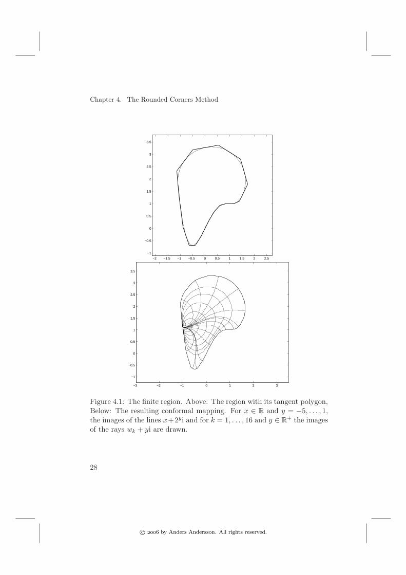
Finite region

Here, we construct a mapping function from the upper half-plane to aregion bounded below by the curve

z = x+ iy, y = x4 − 2x3 + 2x (4.18)

27



−2 −1.5 −1 −0.5 0 0.5 1 1.5 2 2.5

−1

−0.5

0

0.5

1

1.5

2

2.5

3

3.5

−3 −2 −1 0 1 2 3

−1

−0.5

0

0.5

1

1.5

2

2.5

3

3.5

Figure 4.1: The finite region. Above: The region with its tangent polygon,Below: The resulting conformal mapping. For x ∈ R and y = −5, . . . , 1,the images of the lines x+2yi and for k = 1, . . . , 16 and y ∈ R

+ the imagesof the rays wk + yi are drawn.

28


4.4. Examples

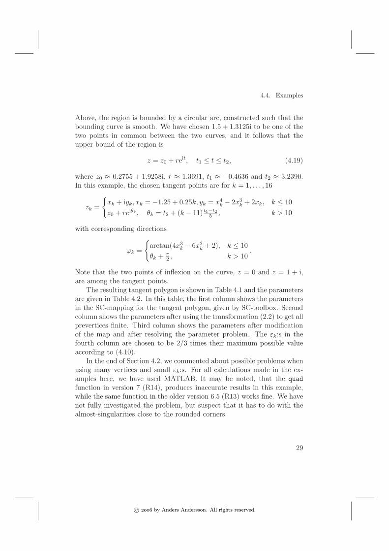
Above, the region is bounded by a circular arc, constructed such that thebounding curve is smooth. We have chosen 1.5 + 1.3125i to be one of thetwo points in common between the two curves, and it follows that theupper bound of the region is

z = z0 + reit, t1 ≤ t ≤ t2, (4.19)

where z0 ≈ 0.2755 + 1.9258i, r ≈ 1.3691, t1 ≈ −0.4636 and t2 ≈ 3.2390.In this example, the chosen tangent points are for k = 1, . . . , 16

zk =

xk + iyk, xk = −1.25 + 0.25k, yk = x4k − 2x3

k + 2xk, k ≤ 10

z0 + reiθk , θk = t2 + (k − 11) t1−t25 , k > 10

with corresponding directions

ϕk =

arctan(4x3k − 6x2

k + 2), k ≤ 10

θk + π2 , k > 10

.

Note that the two points of inflexion on the curve, z = 0 and z = 1 + i,are among the tangent points.

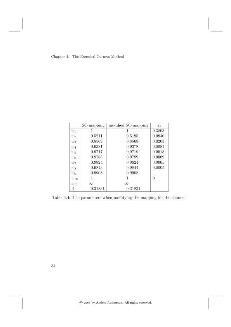
The resulting tangent polygon is shown in Table 4.1 and the parametersare given in Table 4.2. In this table, the first column shows the parametersin the SC-mapping for the tangent polygon, given by SC-toolbox. Secondcolumn shows the parameters after using the transformation (2.2) to get allprevertices finite. Third column shows the parameters after modificationof the map and after resolving the parameter problem. The εk:s in thefourth column are chosen to be 2/3 times their maximum possible valueaccording to (4.10).

In the end of Section 4.2, we commented about possible problems whenusing many vertices and small εk:s. For all calculations made in the ex-amples here, we have used MATLAB. It may be noted, that the quad

function in version 7 (R14), produces inaccurate results in this example,while the same function in the older version 6.5 (R13) works fine. We havenot fully investigated the problem, but suspect that it has to do with thealmost-singularities close to the rounded corners.

29



tangent points tangent polygon verticesk zk ϕk z′k αk

1 −1.0000 + 1.0000i 4.8367 −0.8837 + 0.0696i 0.939122 −0.7500 − 0.3398i 5.0280 −0.6365 − 0.6875i 0.600463 −0.5000 − 0.6875i 0 −0.3925 − 0.6875i 0.681224 −0.2500 − 0.4648i 1.0015 −0.1696 − 0.3393i 0.966375 0 1.1071 0.1625 + 0.3250i 1.022706 0.2500 + 0.4727i 1.0358 0.3807 + 0.6932i 1.079727 0.5000 + 0.8125i 0.7854 0.6193 + 0.9318i 1.153598 0.7500 + 0.9727i 0.3029 0.8375 + 1.0000i 1.096419 1.0000 + 1.0000i 0 1.1696 + 1.0000i 0.86873

10 1.2500 + 1.0352i 0.4124 1.3925 + 1.0975i 0.7788611 1.5000 + 1.3125i 1.1071 1.7377 + 1.7878i 0.7642812 1.5924 + 2.2990i 1.8477 1.4471 + 2.8102i 0.7642813 0.9950 + 3.0895i 2.5882 0.5429 + 3.3688i 0.7642814 0.0207 + 3.2699i 3.3288 −0.5014 + 3.1710i 0.7642815 −0.8201 + 2.7457i 4.0693 −1.1388 + 2.3205i 0.7642816 −1.0871 + 1.7915i 4.8098 −1.0444 + 1.3556i 0.99144

Table 4.1: The tangent points and tangent polygon vertices for the finiteregion

30


4.4. Examples

Parametersin after Moebius after rounding

SC-map transform (2.2) the corners εk

w1 −1 −1 −1 0.0207w2 −0.9359 −0.9379 −0.9363 0.0006w3 −0.9340 −0.9361 −0.9344 0.0006w4 −0.9201 −0.9232 −0.9212 0.0043w5 −0.7317 −0.7634 −0.7567 0.0532w6 −0.4386 −0.5616 −0.5604 0.0492w7 −0.1712 −0.4140 −0.4142 0.0205w8 −0.0425 −0.3525 −0.3534 0.0115w9 0.0347 −0.3181 −0.3182 0.0034w10 0.0586 −0.3078 −0.3078 0.0034w11 0.1382 −0.2746 −0.2747 0.0111w12 0.2477 −0.2316 −0.2318 0.0143w13 0.3694 −0.1871 −0.1873 0.0148w14 0.5505 −0.1266 −0.1269 0.0202w15 1 0 0 0.0422w16 ∞ 1 1 0.3333|A| 0.7907 0.3944 0.3930argA −1.4733 −1.4464 −1.4464

Table 4.2: The parameters when modifying the mapping for the finiteregion

31



Channel

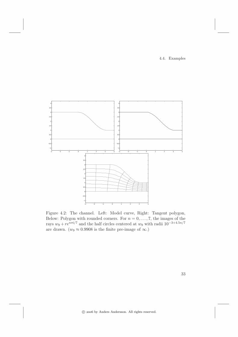
In this example we model a channel with the real axis as a lower bound.As upper bound we take the curve

z = x+ i · y, y =

3 x < 0

2 + cosx 0 ≤ x ≤ π

1 x > π

.

The chosen tangent points on the upper bound have x-values −1, π/8,2π/8, . . . , 7π/8, π + 1. On the lower bound we use the origin as a vertexwith α = 1. Together with the two infinite vertices, the tangent polygonhas 11 vertices. The vertices in the tangent polygon are given in Table4.3.

tangent points verticesk zk ϕk z′k αk

1 4.1416 + i 0 2.9478 + i 1.11632 2.7489 + 1.0761i −0.3655 2.5612 + 1.1480i 1.07963 2.3562 + 1.2929i −0.6155 2.1791 + 1.4181i 1.04154 1.9635 + 1.6173i −0.7459 1.8319 + 1.7389i 1.01265 1.5708 + 2.0000i −0.7854 1.3097 + 2.2611i 0.98746 1.1781 + 2.3827i −0.7459 0.9625 + 2.5819i 0.95857 0.7854 + 2.7071i −0.6155 0.5804 + 2.8520i 0.92048 0.3927 + 2.9239i −0.3655 0.1938 + 3i 0.88379 −1 + 3i 0 −∞ 0

10 0 0 0 111 ∞ 0

Table 4.3: The tangent points and tangent polygon vertices for the channel

The parameters are given in Table 4.4. In this map, the εk:s are set tohalf their maximum possible value according to (4.10).

32


4.4. Examples

−3 −2 −1 0 1 2 3 4

−1

−0.5

0

0.5

1

1.5

2

2.5

3

3.5

4

−3 −2 −1 0 1 2 3 4

−1

−0.5

0

0.5

1

1.5

2

2.5

3

3.5

4

−3 −2 −1 0 1 2 3 4

−1

−0.5

0

0.5

1

1.5

2

2.5

3

3.5

4

Figure 4.2: The channel. Left: Model curve, Right: Tangent polygon,Below: Polygon with rounded corners. For n = 0, . . . , 7, the images of therays w9 + renπi/7 and the half circles centered at w9 with radii 10−3+4.5n/7

are drawn. (w9 ≈ 0.9908 is the finite pre-image of ∞.)

33



SC-mapping modified SC-mapping εk

w1 −1 −1 0.3803w2 0.5211 0.5195 0.0840w3 0.8569 0.8568 0.0203w4 0.9381 0.9378 0.0084w5 0.9717 0.9719 0.0018w6 0.9788 0.9789 0.0009w7 0.9824 0.9824 0.0005w8 0.9843 0.9844 0.0005w9 0.9908 0.9908w10 1 1 0w11 ∞ ∞A 0.31831 0.31831

Table 4.4: The parameters when modifying the mapping for the channel

34


Chapter 5

The Outer Polygon Method

When working with the Schwarz–Christoffel mapping, and especially withthe SC Toolbox [6], it is unavoidable to notice the beautiful smooth curvesthat are the images of lines or circles inside the region that is mapped. Forexample, consider a mapping f from the unit circle to a finite polygon.The image under this mapping of a circle with radius less than but closeto one would be a region bounded by a C∞-curve inside the polygon. Orlet f be a mapping from the upper half-plane to a channel bounded bypolygonal curves. Then the image under f of the region bounded by tworays in the upper half-plane going out from the point on the real axis thatf maps to infinity, would be a channel bounded by smooth curves.

The question arises: Would it be possible, given a simply connectedregion Ω in the complex plane, to find a polygon outside Ω, such that theSchwarz–Christoffel mapping from the upper half–plane or unit circle tothe polygon would map a part of that half–plane or circle on Ω? We willhere show that the answer at least in some cases is affirmative, and sketcha method, “The Outer Polygon method”, to find such a polygon.

We introduce some notation: In the following, we let the letter R eitherthe upper half–plane or the unit circle. We also use the notation Rε withthe following meaning: In the case R is the upper half–plane, we let

Rε = z ∈ C : βπ ≤ arg(z − a) ≤ (1 − ε)πfor some a ∈ R and some 0 ≤ β ≤ ε; if R is the unit circle,

Rε = z ∈ C : |z| ≤ 1 − ε.We note that there exist a conformal mapping gε from R to Rε, where

gε(z) =

(

e−iβπ(z − a))1/(1−ε)

, R is the upper half–plane,

z/(1 − ε), R is the unit circle.

35


Chapter 5. The Outer Polygon Method

(ε− β)π βπa

Rεε Rε

Figure 5.1: The region Rε in the upper half–plane (left) and unit cir-cle(right).

Definition 5.1. Given a simply connected region Ω with smooth boundarycurve Γ, an n-sided outer polygon P

Ω is a polygon with the followingproperties:

• P Ω ⊃ Ω.

• For some Rε, the Schwarz–Christoffel mapping s from R to P Ω maps

Rε conformally on a region with boundary curve C, such that then-sided tangent polygons PC and PΓ are identical.

If an outer polygon can be found, s gε is an approximate conformalmapping from R to Ω, and the Fréchet distance between C and Γ is givenby Theorem 3.2.

5.1 Finding the Outer Polygon

As indicated in the above definition, a good approximation of an outerpolygon can in some cases be found, using the tangent polygons describedin chapter 3. Suppose that Ω is bounded by a smooth curve Γ. We firstturn Γ into a ctp by equipping it with tangent points according to definition3.2, and construct its tangent polygon PΓ. The sides in PΓ correspondingto points of inflexion on Γ are called sides of inflexion.

Let P be an approximation of the polygon P Ω in definition 5.1, with

the same number of sides as the polygon PΓ and with all sides exceptthe sides of inflexion parallel to their counterparts in PΓ. Let further s

36


5.1. Finding the Outer Polygon

be the Schwarz–Christoffel mapping that maps R on P , and let C be theboundary curve of the region s(Rε). We now turn C into a ctp, by choosingtangent points on it where its direction is the same as the direction of Γ.In a point of inflexion where the direction of Γ reaches a local maximumor minimum, this is impossible since the direction of C will not reach thisextreme. But as required, the corresponding point of inflexion on C is atangent point.

In the case of a channel, C is not approaching infinity as a straightline, and can therefore not, according to definition 3.2 be a ctp, but sinceit converges quite fast to its asymptotes, Theorem 2.2, we can extend theidea a little bit and use the asymptotes as tangents in ∞, and so constructa tangent polygon PC .

We will later consider the case ε = 0, and if so, we let PC = C = P .

PΓ and PC are not parallel, since the direction of Γ and C differ in thepoints of inflexion, but with a method similar to that in Section 4.2, wecan find an approximation to the outer polygon P o

Ω. The main differenceis that the direction of the sides of inflexion must be one of the adjustableparameters in the outer polygon.

Assume that PΓ, P and PC are n-sided polygons with side–lengthsLk,Γ, Lk,P and Lk,C for k = 1, . . . , n. As in Section 4.2, we let in the caseof a channel, the channel width at the ends replace two of the polygon’sside–lengths. Assume further that the sides numbered n1, . . . , nm are sidesof inflexion, and that their angular directions are ϕnj ,Γ, ϕnj ,P and ϕnj ,C

for j = 1, . . . ,m. Let

LΓ = L2,Γ, . . . , Ln−1,Γ,

LP = L2,P , . . . , Ln−1,P ,

LC = L2,C , . . . , Ln−1,C

and further

ϕΓ = ϕn1,PΓ, . . . , ϕnm,PΓ

,

ϕP = ϕn1,P , . . . , ϕnm,P ,

ϕC = ϕn1,PC, . . . , ϕnm,PC

.

37



A good approximation of the outer polygon can now be found by solvingthe equation

F (LP ,ϕP ) = 0, (5.1)

where

F (LP ,ϕP ) = (LPΓ− LPC

,ϕPΓ− ϕPC

). (5.2)

A polygon is determined by all but two of the lengths or directionsof the sides. We have in (5.1) omitted two of the side–lengths but otheralternatives are of course possible.

5.2 The Existence of an Outer Polygon

If we allow polygons with arbitrarily many sides, no outer polygon is infact needed. We can make a polygon with a boundary arbitrarily close toΓ, and with a small ε make the image of Rε coincide arbitrarily well withΩ. But it is also for small ε:s that the existence of an outer polygon canbe proved. We state these observations in two theorems.

Theorem 5.1. Suppose that Ω is a simply connected region bounded bya smooth curve Γ, and that R is either the upper half–plane or the unitcircle. Then for any ε0 > 0, the outer polygon method, with a tangentpolygon PΓ as an approximation of the outer polygon P

Ω, can be used tofind a conformal mapping from R to a region bounded by a smooth curveC, where the Fréchet distance δ(C,Γ) < ε0.

Proof. If Ω is a finite region, we can since Γ is smooth, find a tangentpolygon PΓ such that δ(Γ, PΓ) < ε0/2. Let s be the Schwarz–Christoffelmapping from R to PΓ, and let C be the boundary curve of s(Rε). IfR is the unit circle and Ω a finite region, s is uniformly continuous in R(including the boundary of R), and we can find ε > 0 such that δ(C,PΓ) <ε0/2. Hence δ(C,Γ) < ε0.

If Ω is a channel, R is the upper half–plane and Rε a region boundedby rays from the point a on the real axis, we know from Theorem 2.2 that

38


5.2. The Existence of an Outer Polygon

the rays are mapped on curves with asymptotes parallel to the channelwalls at the ends.

Given ε0 > 0, we can find real numbers 0 < r1 < r∗1 < r∗2 < r2 < ∞such that all prevertices wk are inside any of the intervals [a− r∗2, a− r∗1]and [a + r∗1, a + r∗2], and furthermore, for the curve Cϕ = s(a + teiϕ) andits asymptotes in the tangent polygon PCϕ , we can according to Theorem2.2 choose r∗1 and r∗2 such that the distance δ(Cϕ, PCϕ) < ε0/3 for allt /∈ [r∗1, r

∗2] and for all ϕ ∈ [0, π].

Since s is uniformly continuous on a compact subset of R, we can selectε such that for the boundary curve C = s(a+ teiπε) of s(Rε), the distanceδ(C,Γ) < ε0/3 for t ∈ [r1, r2]. Then,

δ(PC ,Γ) ≤ δ(PC , C) + δ(C,Γ) <2ε03

for t ∈ [r1, r∗1] ∪ [r∗2, r2],

and since the asymptotes in PC are parallel to the channel walls in Γ atthe ends of the channel, δ(PC ,Γ) < 2ε0/3 everywhere outside the interval[r∗1, r

∗2]. Hence,

δ(C,Γ) ≤ δ(C,PC) + δ(PC ,Γ) <ε03

+2ε03

= ε0

outside the interval [r1, r2].

Theorem 5.2. Let x ∈ R2n−2 be a vector containing parameters

w2, . . . , wn−2, |A|, α1, . . . , αn in a Schwarz–Christoffel mapping

s(w) = A

∫ w

w0

∏

k

(ω − wk)αk−1dω +B.

Assume that the region Ω is bounded by a ctp Γ, and let xΓ be the param-eters in the mapping for the tangent polygon PΓ. Define the function

S(x) = (L2, . . . , Ln−1, ϕ1, . . . , ϕn),

where Lk is the length and ϕk is the direction of the kth side in the polygons(R) with parameters x. If the Jacobian

∂S

∂x(xΓ) 6= 0,

then there exist an ε > 0 such that an outer polygon P Ω exists.

39



L1,Γ

L2,Γ

L3,Γ

z1

z2

Figure 5.2: The channel Ω. Its tangent polygon PΓ has side–lengths L1,Γ,L2,Γ and L3,Γ and the approximative outer polygon P has vertices z1 andz2.

Proof. Define the function

G(x, ε) = F (LP ,ϕP )

where P is the polygon s(R) with the parameters x in s. G(xΓ, 0) = 0and

∂G

∂x(xΓ, 0) =

∂S

∂x(xΓ) 6= 0,

so by the implicit function theorem, there exist a neighbourhood |ε| < din which parameters x∗

ε can be found such that G(x∗ε, ε) = 0. Then s(R)

with parameters x∗ε is an outer polygon P

Ω.

Given that the Jacobian meets the conditions in the theorem, the exis-tence of an outer polygon can be guaranteed for small values of ε, i.e. whenRε is very close to R. This can always be accomplished, if we use polygonswith many sides. However, it is the possibility to use much simpler poly-gons with easy calculated Schwarz–Christoffel mappings that motivatesthe outer polygon method.

5.3 Example

We illustrate the idea on a channel, shown in Figure 5.2, similar to the onein Section 4.4. The lower bound is a horizontal line, and we can assume

40


5.3. Example

that it is the real axis. The upper bound is a smooth curve, continuouslydifferentiable, horizontal at the ends, decreasing, and with exactly onepoint of inflexion.

Assume that Ω is this channel with boundary curve Γ, and that itswidth is L1,Γ at the left opening and L3,Γ at the right opening. We turnΓ into a ctp with one tangent point on the real axis, one tangent point ateach of the straight line ends of the upper part, and the final tangent pointin the point of inflexion. Assume that the only side with finite length inthe tangent polygon PΓ, the tangent in the point of inflexion, has lengthL2,Γ and direction ϕ2,Γ.

An approximate outer polygon is a polygonal channel P with the realaxis as lower bound. The upper bound is a 3-sided polygonal curve withfirst and last side horizontal, and with vertices in z1 = x1 + iy1 and z2 =x2 + iy2. We can without loss of generality assume that x1 = 0.

Following the idea described above, we now, using for example theSC-toolbox [6], easily construct a Schwarz–Christoffel mapping function

s(w) = A

∫ w

w0

(ω − w1)α1−1(ω − w2)

α2−1

ω − adω +B, (5.3)

which maps the upper half–plane Π+ conformally into the interior of P .In (5.3), a is the real finite number that is mapped to ∞. The function

επ

a

g(Π+)

Figure 5.3: The region g(Π+)

gε(w) = (w − a)1−ε + a (5.4)

41



maps the upper half-plane on the region above the broken line

z = x+ yi,

y = (a− x) tan επ x < a

y = 0, x ≥ a(5.5)

as shown in figure 5.3. Now the function f = s gε maps the upper half–plane on a region bounded by a curve C of similar shape as Γ, and theright half of the real axis (x ∈ R : x > a) is mapped on the real axis.

For some real wC , C has a point of inflexion f(wC) which can befound numerically or algebraically. A tangent polygon PC is constructedwith the tangent to C in f(wC), the two horizontal asymptotes to theupper boundary and the real axis as sides. Let

L1,C = limw→a−

f(w), L3,C = limw→−∞

f(w),

and finally L2,C be the distance between the point of intersections betweenthe tangent and the horizontal lines y = L1,C and y = L3,C .

The function (5.1) can here take the form

F : (y1, x2, y2) → (L1,C − L1,Γ, L2,C − L2,Γ, L3,C − L3,Γ), (5.6)

and we can use Newton’s method to determine y1, x2 and y2 such that Cand Γ have approximately the same tangent polygon. We have then got afunction f that maps the upper half–plane on a channel, bounded belowby the real axis and above by a curve C that in its point of inflexion hasapproximately the same direction as Γ. The y-limits when x → ±∞ arethe same in C and Γ. By a horizontal translation of C, it is possible tolet the points of inflexion on C and Γ have the same real value. However,because of the different curvature of the curve C near a convex and aconcave vertex, the two points will not coincide.

A numerical result

In this example, Ω is the channel in figure 5.2. Its lower bound is thereal axis, and the upper bound has asymptotes y = 2 and y = 1. Theangular direction in its point of inflexion is 5π/6, i.e. the length of thefinite tangent polygon side L2Γ is 2.

42


5.3. Example

−3 −2.5 −2 −1.5 −1 −0.5 0 0.5 1 1.5

−0.5

0

0.5

1

1.5

2

2.5

Figure 5.4: The channel with its outer polygon

In the function gε in equation (5.4), we use ε = 0.05, and when solv-ing (5.6), we use the tangent polygon PΓ as a starting approximation inNewton’s method. After a few iterations, an outer polygon with verticesin −0.7342 + 2.1053i and 0.4198 + 1.0526i is determined, with inner an-gels 0.7646π and 1.2354π in these vertices. The Schwarz–Christoffel map-ping function s for this polygon, found by SC–toolbox, is approximately

s(w) = 0.3350

∫ w

1

(ω + 1)0.2354(ω − 0.7021)−0.2354

ω − 0.7996dω − 0.7342.

(The constant B in (5.3) is here chosen so that x = 0 in the point ofinflexion on Γ. Many other alternatives are of course possible.)

Then the function g in (6.5) is

g(w) = (w − 0.7996)0.95 + 0.7996,

and f = s g is a conformal mapping from the upper half–plane to thischannel.

43



5.4 Comments

Each step in the Newton iteration requires a solution of the parameterproblem in the map s, i.e. determining the constants A, a, w1 and w2 in(5.3). An alternative to the method described above is of course to usethe equations Lk,C = Lk,Γ to directly determine these constants. However,SC–toolbox solves the parameter problem so fast, and moreover, evaluatesthe integrals with such a speed that the roundabout over the polygon P o

Ω

normally reaches the goal faster.In the description of the method, we have used the pair (Lk, ϕk), i.e.

the length and direction of a polygon side to determine the polygons in-volved in the method. We can of course as well use the polygon’s vertices(xk, yk). This is in fact what we have done in the example, in the outerpolygon.

There is a significant difference in the way an inner curve in the tangentpolygon behaves near convex and concave vertices. At a concave vertexthe inner curve passes quite close to the vertex with a high curvature, whileit at a convex vertex passes far from the vertex with a comparably lowercurvature. The difference is great for acute angles.

Hence, in the numerical example above, the absolute curvature of theresulting curve is greater near the concave vertex than near the convexvertex, and the point of inflexion, z = 1.3349i is quite close to the former.

44


Chapter 6

The Zipper Method

6.1 The Zipper algorithms

In [5], a class of algorithms for conformal mappings are described, algo-rithms which are built on the idea that a slit in the upper half-plane canbe removed, using a simple combination of elementary functions. For anyregion in the complex plane, its boundary curve can be cut into smallpieces, and by an iterated use of such a slit-removing function, where eachpiece of the boundary curve is seen as a slit in the upper half-plane, and ofcourse with some suitable starting and finishing mappings, the boundarycurve can be mapped on the real axis, while the region itself is conformallymapped on the upper half-plane. The elementary functions that are usedin the algorithm can all easily be inverted, and so the algorithms result invery efficient and accurate approximate conformal mappings between theupper half-plane and a simple region.

[5] introduces three different algorithms: the slit algorithm, where theslits are assumed to be straight lines, the zipper algorithm, where theyare assumed to be circular arcs through three of the boundary points, andfinally the simple geodesic algorithm, where the slits are assumed to becircular arcs, orthogonal to the the real axis. Since the geodesic algorithmproduces a conformal mapping that maps the upper half-plane on a regionbounded by a smooth curve, and the smoothness has been in focus ofour interests, we have used this algorithm in our work. Furthermore, theconvergence of the geodesic algorithm is proved in [5].

45


Chapter 6. The Zipper Method

The Geodesic algorithm

Let Ω be the upper half-plane with a vertical slit from the origin up to apoint z = ci. It is obvious that the mapping

sc(z) =√

z2 + c2 (6.1)

removes the slit, and maps Ω conformally on the upper half-plane, giventhat the branch of the square root is chosen such that Im sc(z) > 0 whenIm z > 0. If instead Ω is the upper half-plane with a slit that is a circulararc, orthogonal to the real axis, from the origin to the point z = z0, themapping

gb(z) =z

1 − z/b, b =

|z0|2Re z0

(6.2)

takes Ω into a half-plane with vertical slit of length c = |z0|2 / Im z0, andso fz0

= sc gb maps Ω conformally on the upper half-plane.This function can be used repeatedly to approximately map any curve

C in the upper half-plane orthogonal to the real axis on the real axis. Letz0, . . . , zn be points on C ,where z0 is real and z1, . . . , zn, have positiveimaginary part. We can without loss of generality assume that z0 = 0.Let for k = 1, . . . , n

ϕk = fζk fζk−1

· · · fζ1 , ζj =

zj , j = 1

ϕj−1(zj), j > 1. (6.3)

The function ϕn then “zips” the curve C down on the real axis, and fur-thermore, its inverse

ϕ−1n = f−1

ζ1 · · · f−1

ζn(6.4)

maps a part of the real axis on a smooth curve through z0, . . . , zn, a curvethat is orthogonal to the real axis. Combined with some suitable openingand ending elementary maps, this technique can easily be used to approxi-mately construct a conformal mapping function between any simple regionand the upper half-plane.

For our purposes, it is convenient to consider an infinite region R,bounded below by the real axis and a smooth curve C, orthogonal to thereal axis and with control points z0, . . . , zn+1, where z0 = 0 and zn+1 is a

46


6.2. Constructing the Mapping Function

R

z z0 n+1

Figure 6.1: The region R

real positive number. Like before, z1, . . . , zn are all in the upper half-plane.

We want to construct a conformal mapping between R and the upperhalf-plane, and we therefore use the map ϕn described above. If, in any ofthe maps fζk

, b < ϕk−1(zn+1), the image of zn+1 will move to the negativepart of the real axis, and the image of R will be a finite region. A laterf might move zn+1 back again. However, for all k = 1, . . . , n, ϕk(R) is aregion on the left side of the curve from 0 to ζk+1. Finally, after applyingfζn

, ϕn(zn) = 0 and ϕn(zn+1) is real. We assume that the two points areconnected by a semicircle in the upper half-plane. In the case ϕn(zn+1) ispositive, ϕn(R) is an infinite region above the real axis and this semicircle,otherwise ϕn(R) is the finite region between the semicircle and the realaxis. The function

g(z) =

(

z

1 − z/ϕn(zn+1)

)2

, ϕn(zn+1) < 0

z2

2z − ϕn(zn+1), ϕn(zn+1) > 0

(6.5)

maps this region conformally on the upper half-plane, i.e., ϕ = g ϕn is aconformal mapping from R to the upper half-plane.

6.2 Constructing the Mapping Function

Let Ω be a channel in the complex plane, i.e. an infinite simple regionbounded by two smooth not connected curves. For simplicity, we call

47



Figure 6.2: Channel with indented sides and outer polygon

these curves the upper and lower boundary and name them ΓU and ΓL

respectively. We assume further that ΓU and ΓL go to infinity as parallelstraight lines, i.e. that Ω outside some circle is bounded by parallel straightlines.

As a first measure, we find a conformal mapping s between the upperhalf-plane and a region R with the following properties:

• R is a channel that coincides with Ω outside some circle.

• The boundary of R is smooth in every point where it coincides withthe boundary of Ω.

If Ω has indentations on both sides immediately after the straight lineparallel infinite parts (Figure 6.2), we can let R be a polygon with twoinfinite vertices, and s an ordinary Schwarz–Christoffel mapping. If this isnot the case (Figure 6.3), a polygon with rounded corners and a modifiedSchwarz–Christoffel mapping could be used.

Now, s−1(Ω) is an infinite region, bounded below by a smooth curvethat coincides with the real axis everywhere except from a few (normallytwo) regions where it passes through points with positive imaginary parts.In an informal language, the curve makes a few hills above the real axis,though it is still smooth. Assume that the leftmost of these non-real

48


6.2. Constructing the Mapping Function

Figure 6.3: Channel with outer rounded polygon

J−1 s−1(Ω)

s−1(Ω)

Figure 6.4: The regions s−1(Ω) and J−1 s−1(Ω)

parts of the curve are situated at the interval [a, b] on the real axis. TheJoukowski map

J(z) =z2 − ab

2z − a− b(6.6)

maps the upper half-plane minus a semicircle through a and b on the upperhalf-plane, and its inverse will, with an appropriate selection of branches,map the real axis between a and b on a semi-circle through a and b. Assumefurther that we choose branches, such that

x ∈ R, x < a⇒ J−1(x) ∈ R, J−1(x) < a

x ∈ R, x > b⇒ J−1(x) ∈ R, J−1(x) > b

Im z > 0 ⇒ ImJ−1(z) > 0.

The function J−1 will then map the boundary curve between a and b on a

49



smooth curve above this semi-circle, orthogonal to the real axis at a andb. The rest of the boundary curve will of course be affected, but sincereal numbers outside [a, b] are mapped on real numbers and points in theupper half-plane are mapped on points in the upper half-plane, all othernon-real parts of the curve are still “smooth hills” above the real axis.

A translation by a will take us to the situation described in Section6.1. The function ϕ described there will map the first non-real part of thecurve on the real axis, and leave the others not unchanged, but as new“smooth hills” above the real axis. This can be done repeatedly, until allthe non-real parts are removed, and the region Ω is mapped conformallyon the upper half-plane.

To all the mappings used in the process, we can easily find inverses,and so construct a conformal mapping from the upper half-plane to Ω.

6.3 Examples

Example 1

−6 −4 −2 0 2 4 6

−2

0

2

4

6

8

Figure 6.5: The channel Ω and polygon R.

In this example, we construct a conformal mapping for a channel Ω,

50


6.3. Examples

bounded below by the real axis and above by the curve

z = x+ yi, y =

5, x < −π3 − 2 cosx, −π ≤ x < 02 − cosx, 0 ≤ x < π3, x ≥ π

. (6.7)

On the curved part −π ≤ x ≤ π we put reference points with values xk+ykiwhere xk = π−kπ/10. We let R be the polygonal channel bounded belowby the real axis and above by a polygonal curve with right-angled verticesin the points 5i and 3i.

With the SC-toolbox [6], we find the Schwarz–Christoffel mapping

s(w) = 0.9549

∫ w

1

√ω + 1√

ω + 0.5548(ω + 0.3044)dω, (6.8)

mapping the upper half–plane on R, and as described in Section 6.2, we uses−1 (implemented in the toolbox) to find the constants a and b in the mapJ defined in equation (6.6) and its inverse. We have a = s−1(x0 + y0i) =−30.1921 and b = s−1(x20 + y20i) = −0.3879, and so we can start thegeodesic algorithm with the values zk = J−1(s−1(xk + yki)) − a, given inTable 6.1.

The function ϕ19, defined in equation (6.3), maps the channel on ahalf–circle that intersects the real axis at ϕ19(z20) = −2.3524 · 105 and theorigin. This means that the function g defined in equation (6.5) here is

g(z) =

(

z

1 + z/235243

)2

.

Since ϕ(z20) = gϕ19(z20) = ∞, the curved part of the channel bound-ary is mapped on an infinite part of the negative real axis, something thatmust be taken into consideration, when constructing a mapping from astraight horizontal channel to Ω. We also note that the two points of in-finity at each end of Ω are now mapped to two points on the real axis,B = −3.0441 · 108 and C = −3.2613 · 108. Because of these things, it isdifficult and not very meaningful to make a nice square grid on the half–plane, invert the mappings, and expect the original channel to appear.

51



k xk + yki zk ζk ϕ19(zk)/104 ϕ(zk)/108

0 3.1416+3.0000i 0 0 −1.6237 −3.04201 2.8274+2.9511i 7.9427+14.6098i 7.9427+14.610i −1.6237 −3.04202 2.5133+2.8090i 14.8161+18.3200i −2.3829+23.564i −1.6237 −3.04203 2.1991+2.5878i 21.5077+19.5796i −0.5180+31.123i −1.6237 −3.04204 1.8850+2.3090i 27.7181+18.7751i −0.0273+41.700i −1.6237 −3.04205 1.5708+2.0000i 32.7288+16.2917i 1.3586+56.885i −1.6237 −3.04206 1.2566+1.6910i 36.0034+12.9160i 3.9015+78.861i −1.6237 −3.04207 0.9425+1.4122i 37.5295+ 9.5507i 9.6850+110.59i −1.6237 −3.04208 0.6283+1.1910i 37.7409+ 6.8195i 21.415+155.67i −1.6237 −3.04209 0.3142+1.0489i 37.1932+ 4.9284i 42.956+218.07i −1.6237 −3.0419

10 0+1.0000i 36.3195+ 3.7766i 75.434+306.71i −1.6237 −3.041611 −0.3142+1.0979i 35.2561+ 3.2503i 154.76+433.23i −1.6234 −3.040512 −0.6283+1.3820i 34.0660+ 3.0860i 186.56+752.94i −1.6224 −3.036413 −0.9425+1.8244i 32.8855+ 2.9191i 85.681+1266.9i −1.6194 −3.024614 −1.2566+2.3820i 31.8838+ 2.5815i 52.828+1902.2i −1.6123 −2.996115 −1.5708+3.0000i 31.1773+ 2.1414i 37.156+2665.8i −1.5968 −2.934816 −1.8850+3.6180i 30.7106+ 1.7304i 161.46+3576.0i −1.5641 −2.807217 −2.1991+4.1756i 30.3700+ 1.3752i 330.44+4900.5i −1.4903 −2.531718 −2.5133+4.6180i 30.1001+ 1.0421i 375.15+7322.7i −1.2977 −1.886319 −2.8274+4.9021i 29.9002+ 0.6885i 39.420+ 12976i 0 020 −3.1416+5.0000i 29.8042 −235243 −235243 ∞

Table 6.1: The values of the reference points on the curved part of theboundary after the different mappings

Instead, we can construct a mapping from the channel

Q = x+ yi : x, y ∈ R, 0 ≤ y ≤ 1

to Ω. The function

r(z) =C −B

eπz + 1+ C

maps Q on the upper half–plane in such a way that the point z = i ismapped to infinity, the left end of the channel is mapped to B and theright to C. Hence, the function

F (z) = s(J(ϕ−119 (g−1(r(z))) + a))

is a conformal mapping from Q to Ω.

52


6.3. Examples

−6 −4 −2 0 2 4 6

−2

0

2

4

6

8

Figure 6.6: The image under F of a straight horizontal channel with width1. The horizontal grid lines are images of the lines x+0.1ki, k = 0, . . . , 10and the vertical are images of k + yi, k = 0, . . . , 5, 0 ≤ y ≤ 1.

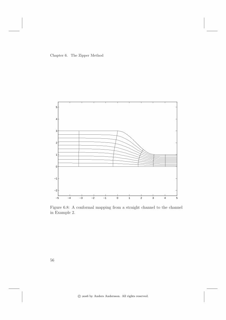
Example 2

In this example, we use the geodesic algorithm to construct a conformalmapping for the region that was treated in section 4.4. This channelrequires a polygon with rounded corners as an outer region for which amodified Schwarz–Christoffel mapping

s = A

∫ w

w0

3∏

k=1

hk(ω) dω

53



−2 −1 0 1 2 3 4 5

−1

−0.5

0

0.5

1

1.5

2

2.5

3

3.5

4

Figure 6.7: The channel and an outer polygon with rounded corners.

is constructed. In s, A = 1/π, w0 = 0.9984 and the factors hk are

h1(ω) =(ω + 0.3449)0.24 + (ω + 1.6551)0.24

2,

h2(ω) =(ω − 0.9580)0.76 − (ω − 0.9716)0.76

2 · 0.76 · 0.0068,

h3(ω) = (ω − 0.9848)−1.

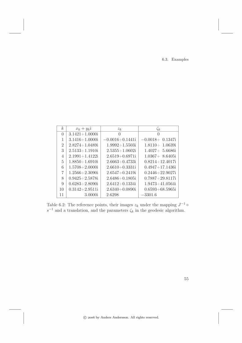
As reference points on the curved part of the boundary, we use thepoints xk +yki, with xk = (11−k)π/10, k = 1, . . . , 11, yk = (2+cos xk)i,and finally x0+y0i = 3.1421+i, the point where the boundary curve meetsthe outer rounded polygon. In the map J defined in equation (6.6), wehave in this example a = s−1(x0 + y0i) = −1.6551 and b = s−1(x11 +y11i) = 0.9747, and so we can start the geodesic algorithm with the valueszk = J−1(s−1(xk + yki)) − a, given in Table 6.2. In the table are also theparameters ζk given, and a picture of the the resulting conformal mappingis shown in Figure 6.8.

54


6.3. Examples

k xk + yki zk ζk0 3.1421+1.0000i 0 01 3.1416+1.0000i −0.0016+0.1441i −0.0018+ 0.1347i2 2.8274+1.0489i 1.9992+1.5503i 1.8110+ 1.0639i3 2.5133+1.1910i 2.5355+1.0602i 1.4027+ 5.6686i4 2.1991+1.4122i 2.6519+0.6971i 1.0367+ 8.6405i5 1.8850+1.6910i 2.6663+0.4733i 0.8214+12.4017i6 1.5708+2.0000i 2.6610+0.3331i 0.4947+17.1436i7 1.2566+2.3090i 2.6547+0.2419i 0.2446+22.9027i8 0.9425+2.5878i 2.6486+0.1805i 0.7887+29.8117i9 0.6283+2.8090i 2.6412+0.1334i 1.9473+41.0564i

10 0.3142+2.9511i 2.6340+0.0890i 0.6593+68.5965i11 3.0000i 2.6298 −3301.6

Table 6.2: The reference points, their images zk under the mapping J−1 s−1 and a translation, and the parameters ζk in the geodesic algorithm.

55



−5 −4 −3 −2 −1 0 1 2 3 4 5

−2

−1

0

1

2

3

4

5

Figure 6.8: A conformal mapping from a straight channel to the channelin Example 2.

56


Chapter 7

Summary and Conclusions

We have in this work treated three different methods for constructingconformal mappings for regions bounded by smooth curves. The researchwas first motivated by the difficulty to find a mapping for such a region withsufficient control of the boundary, using one of the traditional methods.Like all the traditional methods, our methods have their advantages anddrawbacks.

The rounded corners method described in chapter 4 gives a good controlover the boundary curve, since the direction is preserved in all the tangentpoints and varies monotonously between them. The main problem withthe method is that the complexity of the mapping function increases withthe number of tangent points, and can soon enough reach a level wherethe calculation of the integrals is very time-consuming or error-prone.

However, thanks to the control of the direction mention above, aston-ishing good results can be achieved with surprisingly few tangent points.Secondly, we are not sure that the integration method used in this work,adaptive Simson’s quadrature as implemented in Matlab’s quad-function,is the fastest and most appropriate numerical integration method for thefunctions we work with.

With the outer polygon method described in chapter 5, we can makeuse of the fast Gauss-Jacobi quadrature as it is implemented in SC-toolbox[6], and have therefore access to fast calculation of function values, bothwhen determining the function parameters, i.e. the vertices of the outerpolygon, and when using the resulting function. We also note the infi-nite regularity of the boundary curve. If s is a Schwarz–Christoffel map-ping from the region R to a polygon, then s(Rε) is a region boundedby a C∞–curve for any ε > 0. The two other methods produce just C1

boundary curves.

57


Chapter 7. Summary and Conclusions

One obvious disadvantage with the method is the limited control of thedirection, especially when, as described in the introduction, it is requiredthat channel walls are parallel at the ends. In those cases, we have toaccept just an approximate parallelity.

It must also be mentioned, that more research is needed on this method.In a more complicated problem than that described in 5.3, we don’t yetknow if a nontrivial outer polygon exists, and if it does, under whichconditions the Newton iteration converges to that polygon.

The zipper method, described in chapter 6, uses a completely differentidea. The calculation of function values is fast, even if many thousandsof control points are used. We have no total control of the direction inthe control points, but the convergence when using more and more pointsis shown in [5] and since we without difficulty can use very many points,the method seems to be a good alternative. Note also that if needed,parallelity at the ends is here guaranteed by the way we use the geodesicalgorithm.

However, numerical problems can occur. As demonstrated in the sim-ple numerical example, the parameters tend to grow very large, and aninteresting part of the channel corresponds to a small region far away inthe half–plane. This means that it could in some cases be difficult to meeta required accuracy when working in double precision, especially if theboundary is complicated and many reference points are needed. Even inthe simple example above, noticeable inaccurate values appear if we try touse the function F on numbers with real values greater than about 15. Ifsuch calculations are required, a better machine precision is needed.

7.1 Suggestions for future work

When working with numerical methods, you find yourself in a border-land between mathematical and experimental sciences. A lot of successfulexperiments with a certain method can convince you that an iterative al-gorithm always results in an appropriate function, and of course, that sucha function exists. But the method can still resist your attempts to proveconvergence or existence.

This is the situation with the rounded corners method. We have been

58


7.1. Suggestions for future work

able to prove the existence of a solution to the parameter problem for justvery modest roundings of the corners, roundings so small that a redeter-mination of the parameters is really not needed. The experimental resultshave convinced us of the existence in a much wider range of situations, butwe have not yet been able to produce a proof for global or next–to–globalexistence.

As mentioned above, there is a lot left to do with the outer polygonmethod. In this work, we just present the idea, and the preliminary sug-gestion that the concept of tangent polygons also in this method may bea useful tool, when solving the parameter problem. But there is lot ofwork still remaining. It must be investigated if an outer polygon alwaysexist, and for which problems the method is useful. Our experiments withit shows that you soon run into problems when trying it on more com-plicated regions, where the curvature of the boundary curve changes signseveral times.

59


Bibliography

[1] Helmut Alt and Michael Godau. Computing the Fréchet distancebetween two polygonal curves. Internat. J. Comput. Geom. Appl., 5(1-2):75–91, 1995. Eighth Annual ACM Symposium on ComputationalGeometry (Berlin, 1992).

[2] Petter Bjørstad and Eric Grosse. Conformal mapping of circular arcpolygons. SIAM J. Sci. Statist. Comput., 8(1):19–32, 1987.

[3] James Corones and Rober Krueger. Obtaining scattering kernels usinginvariant imbedding. J. Math. Anal. Appl., 95(2):393–415, 1983.

[4] R.T. Davis. Numerical methods for coordinate generation based onSchwarz-Christoffel transformations. In 4th AIAA Comput. Fluid Dy-namic Conf., pages 1–15, Williamsburg, VA, 1979.

[5] Marshall D.E. and S. Rohde. Convergence of the zipper al-gorithm for conformal mapping. Preprint available fromhttp://www.math.washington.edu/~marshall/preprints/zipper.pdf.

[6] T. A. Driscoll. Schwarz–Christoffel toolbox for Matlab. Availablefrom http://www.math.udel.edu/~driscoll/SC/.

[7] Tobin A. Driscoll and Lloyd N. Trefethen. Schwarz-Christoffel map-ping, volume 8 of Cambridge Monographs on Applied and Computa-tional Mathematics. Cambridge University Press, Cambridge, 2002.

[8] Peter Henrici. Applied and computational complex analysis. Vol.3. Pure and Applied Mathematics (New York). John Wiley &Sons Inc., New York, 1986. Discrete Fourier analysis—Cauchyintegrals—construction of conformal maps—univalent functions, AWiley-Interscience Publication.

60


Bibliography

[9] Peter Henrici. Applied and computational complex analysis. Vol.1. Wiley Classics Library. John Wiley & Sons Inc., New York,1988. Power series—integration—conformal mapping—location of ze-ros, Reprint of the 1974 original, A Wiley-Interscience Publication.

[10] L.H. Howell. Computation of Conformal Maps by Modified Schwarz-Christoffel Transformations. PhD thesis, MIT, 1990.

[11] Louis H. Howell. Numerical conformal mapping of circular arc poly-gons. J. Comput. Appl. Math., 46(1-2):7–28, 1993. Computationalcomplex analysis.

[12] Prem K. Kythe. Computational conformal mapping. BirkhäuserBoston Inc., Boston, MA, 1998.

[13] Börje Nilsson. Acoustic transmission in curved ducts with variouscross-sections. Proc. R. Soc. Lond. A, 458:1555–1574, 2002.

[14] Börje Nilsson and Olle Brander. The propagation of sound in cylin-drical ducts with mean flow and bulk reacting lining. iv. IMA J. Appl.Math., 27:263–289, 1981.

[15] Günter Rote. Computing the Fréchet distance between piecewisesmooth curves. To appear in Computational Geometry, Theory andApplications, 2005.

[16] Roland Schinzinger and Patricio A. A. Laura. Conformal mapping:methods and applications. Elsevier Science Publishers B.V., Amster-dam, 1991.

[17] Kenneth Stephenson. The approximation of conformal structuresvia circle packing. In Computational methods and function theory1997 (Nicosia), volume 11 of Ser. Approx. Decompos., pages 551–582.World Sci. Publishing, River Edge, NJ, 1999.

[18] Lloyd N. Trefethen. Numerical computation of the Schwarz-Christoffel transformation. SIAM J. Sci. Statist. Comput., 1(1):82–102, 1980.

61


Bibliography

[19] Lloyd N. Trefethen, editor. Numerical conformal mapping. North-Holland Publishing Co., Amsterdam, 1986. Reprint of J. Comput.Appl. Math. 14 (1986), no. 1-2.

62



Växjö UniversityDepartment of Mathematics and Systems Engineering

issn - isrn vxu-msi-ma-r----se

Date post:	12-Mar-2022
Category:	Documents
Upload:	others
View:	10 times
Download:	0 times

Numerical Conformal Mappings for Regions Bounded by - DiVA

Documents