Page 1
Numerical Evaluation of One-Loop
Scattering Amplitudes for e−e+ → e−e+γ
Giovanni Ossola
New York City College of TechnologyCity University of New York (CUNY)
USTRON’09 – MATTER TO THE DEEPEST
Recent Developments in Physics of Fundamental Interactions
Ustron, Poland – September 11-16, 2009
Giovanni Ossola (City Tech) OPP Reduction September 2009 1 / 30
Page 2
Outline
1 Motivation & Introduction
2 A few comments on the OPP method
3 Work in Progress and New Results
4 NLO QED corrections to e−e+ → e−e+γ, e−e+ → µ
−µ
+γ
Giovanni Ossola (City Tech) OPP Reduction September 2009 2 / 30
Page 3
Summary and Conclusions
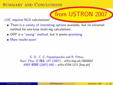
from USTRON 2007LHC requires NLO calculations!
There is a variety of interesting options available, but no universalmethod for one-loop multi-leg calculations
OPP is a “young” method, but it seems promising
More results soon!
G. O., C. G. Papadopoulos and R. Pittau
Nucl. Phys. B 763, 147 (2007) – arXiv:hep-ph/0609007JHEP 0707 (2007) 085 – arXiv:0704.1271 [hep-ph]
Giovanni Ossola (City Tech) OPP Reduction September 2009 3 / 30
Page 4
Progress in 2005-2009
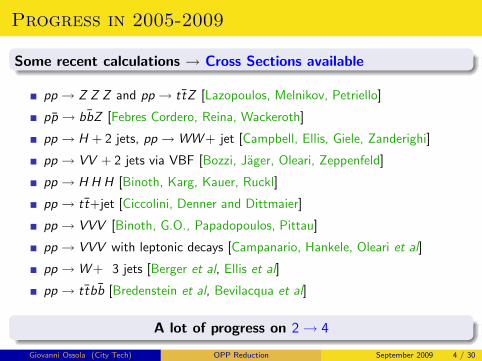
Some recent calculations → Cross Sections available
pp → Z Z Z and pp → ttZ [Lazopoulos, Melnikov, Petriello]
pp → bbZ [Febres Cordero, Reina, Wackeroth]
pp → H + 2 jets, pp → WW+ jet [Campbell, Ellis, Giele, Zanderighi]
pp → VV + 2 jets via VBF [Bozzi, Jager, Oleari, Zeppenfeld]
pp → H H H [Binoth, Karg, Kauer, Ruckl]
pp → tt+jet [Ciccolini, Denner and Dittmaier]
pp → VVV [Binoth, G.O., Papadopoulos, Pittau]
pp → VVV with leptonic decays [Campanario, Hankele, Oleari et al]
pp → W+ 3 jets [Berger et al, Ellis et al]
pp → ttbb [Bredenstein et al, Bevilacqua et al]
A lot of progress on 2 → 4
Giovanni Ossola (City Tech) OPP Reduction September 2009 4 / 30
Page 5
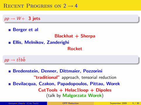
Recent Progress on 2 → 4
pp → W + 3 jets
Berger et al
Blackhat + Sherpa
Ellis, Melnikov, Zanderighi
Rocket
pp → ttbb
Bredenstein, Denner, Dittmaier, Pozzorini
“traditional” approach, tensorial reduction
Bevilacqua, Czakon, Papadopoulos, Pittau, Worek
CutTools + Helac1loop + Dipoles(talk by Malgorzata Worek)
Giovanni Ossola (City Tech) OPP Reduction September 2009 5 / 30
Page 6
OPP Method
Three years ago (Sept.2006), we proposed a new method for the numericalevaluation of scattering amplitudes, based on a decomposition at theintegrand level.
Some of the advantages:
Universal - applicable to any process
Simple - based on basic algebraic properties
Automatizable - easy to implement in a computer code
Final Task
Produce a MULTI-PROCESS fully automatized NLO generator
Giovanni Ossola (City Tech) OPP Reduction September 2009 6 / 30
Page 7
“Standing on the shoulders of giants”
1 Passarino-Veltman Reduction to Scalar Integrals
M =∑
i
di Boxi +∑
i
ci Trianglei
+∑
i
bi Bubblei +∑
i
ai Tadpolei + R ,
Set the basis for our NLO calculationsExploits the Lorentz structure
2 Pittau/del Aguila Recursive Tensorial ReductionExpress qµ =
∑
i Gi ℓiµ , ℓi
2 = 0The generated terms might reconstruct denominators Di
or vanish upon integration
3 “Cut-based” Techniques (Bern, Dixon, Dunbar, Kosower in ’94)direct extraction of the coefficients of the scalar integral
Pigmaei gigantum humeris impositi plusquam ipsi gigantes vident
Giovanni Ossola (City Tech) OPP Reduction September 2009 7 / 30
Page 8
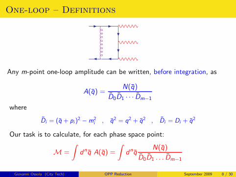
One-loop – Definitions
Any m-point one-loop amplitude can be written, before integration, as
A(q) =N(q)
D0D1 · · · Dm−1
where
Di = (q + pi )2 − m2
i , q2 = q2 + q2 , Di = Di + q2
Our task is to calculate, for each phase space point:
M =
∫
dnq A(q) =
∫
dnqN(q)
D0D1 . . . Dm−1
Giovanni Ossola (City Tech) OPP Reduction September 2009 8 / 30
Page 9
The traditional “master” formula
∫
A =
m−1∑
i0<i1<i2<i3
d(i0i1i2i3)
∫
1
Di0Di1Di2Di3
+
m−1∑
i0<i1<i2
c(i0i1i2)
∫
1
Di0Di1Di2
+m−1∑
i0<i1
b(i0i1)
∫
1
Di0Di1
+m−1∑
i0
a(i0)
∫
1
Di0
+ rational terms
Giovanni Ossola (City Tech) OPP Reduction September 2009 9 / 30
Page 10
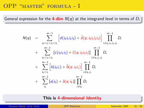
OPP “master” formula - I
General expression for the 4-dim N(q) at the integrand level in terms of Di
N(q) =
m−1∑
i0<i1<i2<i3
[
d(i0i1i2i3) + d(q; i0i1i2i3)]
m−1∏
i 6=i0,i1,i2,i3
Di
+
m−1∑
i0<i1<i2
[c(i0i1i2) + c(q; i0i1i2)]
m−1∏
i 6=i0,i1,i2
Di
+
m−1∑
i0<i1
[
b(i0i1) + b(q; i0i1)]
m−1∏
i 6=i0,i1
Di
+
m−1∑
i0
[a(i0) + a(q; i0)]
m−1∏
i 6=i0
Di
This is 4-dimensional Identity
Giovanni Ossola (City Tech) OPP Reduction September 2009 10 / 30
Page 11
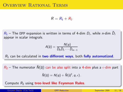
Overview Rational Terms
R = R1 + R2
R1 – The OPP expansion is written in terms of 4-dim Di , while n-dim Di
appear in scalar integrals.
A(q) =N(q)
D0D1 · · · Dm−1
R1 can be calculated in two different ways, both fully automatized.
R2 – The numerator N(q) can be also split into a 4-dim plus a ǫ-dim part
N(q) = N(q) + N(q2, q, ǫ) .
Compute R2 using tree-level like Feynman Rules.
Giovanni Ossola (City Tech) OPP Reduction September 2009 11 / 30
Page 12
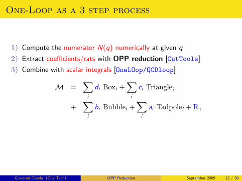
One-Loop as a 3 step process
1) Compute the numerator N(q) numerically at given q
2) Extract coefficients/rats with OPP reduction
3) Combine with scalar integrals
M =∑
i
di Boxi +∑
i
ci Trianglei
+∑
i
bi Bubblei +∑
i
ai Tadpolei + R ,
Giovanni Ossola (City Tech) OPP Reduction September 2009 12 / 30
Page 13
One-Loop as a 3 step process
1) Compute the numerator N(q) numerically at given q
2) Extract coefficients/rats with OPP reduction [CutTools]
3) Combine with scalar integrals [OneLOop/QCDloop]
M =∑
i
di Boxi +∑
i
ci Trianglei
+∑
i
bi Bubblei +∑
i
ai Tadpolei + R ,
Giovanni Ossola (City Tech) OPP Reduction September 2009 12 / 30
Page 14
One-Loop as a 3 step process
1) Compute the numerator N(q) numerically at given q [???]
2) Extract coefficients/rats with OPP reduction [CutTools]
3) Combine with scalar integrals [OneLOop/QCDloop]
M =∑
i
di Boxi +∑
i
ci Trianglei
+∑
i
bi Bubblei +∑
i
ai Tadpolei + R ,
What about the numerator N(q) ?
Giovanni Ossola (City Tech) OPP Reduction September 2009 12 / 30
Page 15
A real proof of concept
van Hameren, Papadopoulos, Pittau – arXiv:0903.4665 [hep-ph]
1) numerator N(q) numerically with HELAC-1loop
2) coefficients via OPP reduction with CutTools
3) scalar integrals with OneLOop/QCDloop
Fully Automated numerical evaluation of ANY one-loop amplitude
All 6-particle processes in the Les Houches 2007 “Wish List’
uu → ttbb gg → ttbb uu → W +W−bb gg → W +W−bb
uu → bbbb gg → bbbb ud → W +ggg uu → Zggg
uu → ttgg gg → ttgg
Czakon, Papadopoulos, Worek – arXiv:0905.0883 [hep-ph]
Dipoles: Automated Dipole Subtraction within HELACGiovanni Ossola (City Tech) OPP Reduction September 2009 13 / 30
Page 16
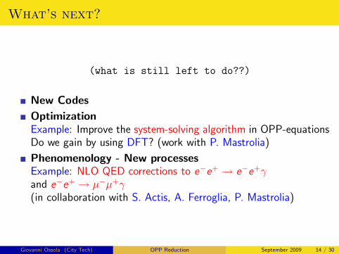
What’s next?
(what is still left to do??)
New Codes
OptimizationExample: Improve the system-solving algorithm in OPP-equationsDo we gain by using DFT? (work with P. Mastrolia)
Phenomenology - New processesExample: NLO QED corrections to e−e+ → e−e+
γ
and e−e+ → µ−µ
+γ
(in collaboration with S. Actis, A. Ferroglia, P. Mastrolia)
Giovanni Ossola (City Tech) OPP Reduction September 2009 14 / 30
Page 17
NLO QED corrections to e−e+ → e−e+γ
During the last few years, there has been a significant progress in reducing
the theoretical uncertainty in Bhabha generators used at presently running
e+e− colliders down to 0.1%
NNLO QED calculations are essential to establish the theoretical accuracy
of existing generators and, if necessary, to improve it below 0.1%
In particular, the one-loop corrections to single hard bremsstrahlung should
be calculated for full Bhabha scattering, to get a better control of the
theoretical precision
G. Balossini, C. Bignamini, C. M. Carloni Calame, G. Montagna,O. Nicrosini and F. Piccinini
“Mini-review on Monte Carlo programs for Bhabha scattering,”
talk presented at Loops and Legs in Quantum Field Theory 2008
Giovanni Ossola (City Tech) OPP Reduction September 2009 15 / 30
Page 18
Tree-level diagrams
QED tree-level diagrams for e−e+ → e−e+γ (full set)and e−e+ → µ−µ+γ (first line only)
Giovanni Ossola (City Tech) OPP Reduction September 2009 16 / 30
Page 19
One-loop diagrams
Representative one-loop diagrams for e−e+ → e−e+γ:
2d2c2b2a
2e 2f 2g
QGRAF generates 38 one-loop diagrams for the process e−e+ → µ−µ+γ
and 76 diagrams for the process e−e+ → e−e+γ
Giovanni Ossola (City Tech) OPP Reduction September 2009 17 / 30
Page 20
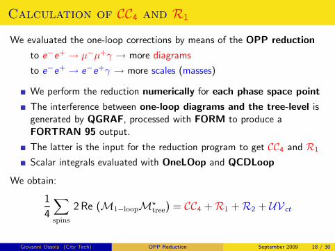
Calculation of CC4 and R1
We evaluated the one-loop corrections by means of the OPP reduction
to e−e+ → µ−µ+γ → more diagrams
to e−e+ → e−e+γ → more scales (masses)
We perform the reduction numerically for each phase space point
The interference between one-loop diagrams and the tree-level isgenerated by QGRAF, processed with FORM to produce aFORTRAN 95 output.
The latter is the input for the reduction program to get CC4 and R1
Scalar integrals evaluated with OneLOop and QCDLoop
We obtain:
1
4
∑
spins
2 Re (M1−loopM⋆
tree) = CC4 + R1 + R2 + UVct
Giovanni Ossola (City Tech) OPP Reduction September 2009 18 / 30
Page 21
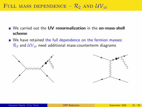
Full mass dependence – R2 and UVct
We carried out the UV renormalization in the on-mass-shellscheme
We have retained the full dependence on the fermion masses:R2 and UVct need additional mass-counterterm diagrams
Giovanni Ossola (City Tech) OPP Reduction September 2009 19 / 30
Page 22
Checks that we performed
1 Two independent calculations
A) CutTools for the reduction + QCDLoop for scalar integralsB) independent code for the reduction + OneLOop for scalar integrals
2 “N = N” test (done by CutTools)
3 Double precision vs Multiple precision
4 Complete cancellation of UV and IR poles
5 Stability test on quasi-collinear configuration
Giovanni Ossola (City Tech) OPP Reduction September 2009 20 / 30
Page 23
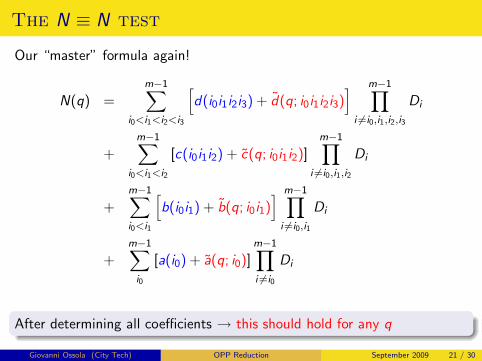
The N ≡ N test
Our “master” formula again!
N(q) =
m−1∑
i0<i1<i2<i3
[
d(i0i1i2i3) + d(q; i0i1i2i3)]
m−1∏
i 6=i0,i1,i2,i3
Di
+
m−1∑
i0<i1<i2
[c(i0i1i2) + c(q; i0i1i2)]
m−1∏
i 6=i0,i1,i2
Di
+
m−1∑
i0<i1
[
b(i0i1) + b(q; i0i1)]
m−1∏
i 6=i0,i1
Di
+m−1∑
i0
[a(i0) + a(q; i0)]m−1∏
i 6=i0
Di
After determining all coefficients → this should hold for any q
Giovanni Ossola (City Tech) OPP Reduction September 2009 21 / 30
Page 24
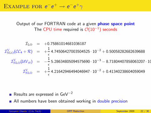
Example for e−e+ → e−e+γ
Output of our FORTRAN code at a given phase space pointThe CPU time required is O(10−1) seconds
ILO = +0.75861014681036187
IV
NLO(CC4 + R) = +1
ǫ4.74506427003504525 · 10−2 + 0.50058282682639688
IV
NLO(UVct) = −1
ǫ5.28634805094575690 · 10−3 − 8.71804407858063207 · 10
IV
NLO = +1
ǫ4.21642946494046947 · 10−2 + 0.41340238604059049
Results are expressed in GeV−2
All numbers have been obtained working in double precision
Giovanni Ossola (City Tech) OPP Reduction September 2009 22 / 30
Page 25
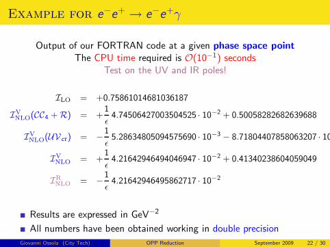
Example for e−e+ → e−e+γ
Output of our FORTRAN code at a given phase space pointThe CPU time required is O(10−1) seconds
Test on the UV and IR poles!
ILO = +0.75861014681036187
IV
NLO(CC4 + R) = +1
ǫ4.74506427003504525 · 10−2 + 0.50058282682639688
IV
NLO(UVct) = −1
ǫ5.28634805094575690 · 10−3 − 8.71804407858063207 · 10
IV
NLO = +1
ǫ4.21642946494046947 · 10−2 + 0.41340238604059049
IR
NLO = −1
ǫ4.21642946495862717 · 10−2
Results are expressed in GeV−2
All numbers have been obtained working in double precision
Giovanni Ossola (City Tech) OPP Reduction September 2009 22 / 30
Page 26
Example for e−e+ → µ−µ
+γ
Virtual part IVNLO as a function of the energy E−of the outgoing muon:
the muon is (almost) parallel or antiparallel to the photon momentum
0.01
0.012
0.014
0.016
0.018
0.02
0.022I
V NLO
[GeV
−2]
0.1 0.2 0.3 0.4 0.5
E− [GeV]
There are no istabilities(work done in double precision)
Giovanni Ossola (City Tech) OPP Reduction September 2009 23 / 30
Page 27
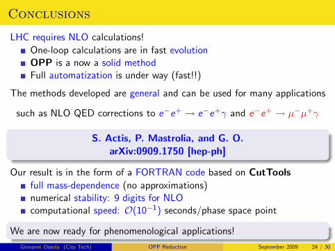
Conclusions
LHC requires NLO calculations!
One-loop calculations are in fast evolutionOPP is a now a solid methodFull automatization is under way (fast!!)
Giovanni Ossola (City Tech) OPP Reduction September 2009 24 / 30
Page 28
Conclusions
LHC requires NLO calculations!
One-loop calculations are in fast evolutionOPP is a now a solid methodFull automatization is under way (fast!!)
The methods developed are general and can be used for many applications
such as NLO QED corrections to e−e+ → e−e+γ and e−e+ → µ−µ+γ
S. Actis, P. Mastrolia, and G. O.
arXiv:0909.1750 [hep-ph]
Our result is in the form of a FORTRAN code based on CutTools
full mass-dependence (no approximations)numerical stability: 9 digits for NLOcomputational speed: O(10−1) seconds/phase space point
We are now ready for phenomenological applications!
Giovanni Ossola (City Tech) OPP Reduction September 2009 24 / 30
Page 29
Sideboard
EXTRA SLIDES
Giovanni Ossola (City Tech) OPP Reduction September 2009 25 / 30
Page 30
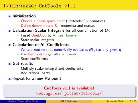
Intermezzo: CutTools v1.1
Initialization- Choose a phase-space point (“extended” kinematics)- Define denominators Di : momenta and masses
Calculation Scalar Integrals for all combination of Di .- I used OneLOop by A. van Hameren- Store scalar integrals
Calculation of All Coefficients- Write a routine that numerically evaluates N(q) at any given q
- Use CutTools to get all coefficients- Store coefficients
Get results- Multiply scalar integral and coefficients- Add rational parts
Repeat for a new PS point
CutTools v1.1 is available!www.ugr.es/ pittau/CutTools/
Giovanni Ossola (City Tech) OPP Reduction September 2009 26 / 30
Page 31
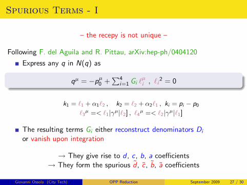
Spurious Terms - I
– the recepy is not unique –
Following F. del Aguila and R. Pittau, arXiv:hep-ph/0404120
Express any q in N(q) as
qµ = −pµ
0 +∑4
i=1 Gi ℓµ
i , ℓi2 = 0
k1 = ℓ1 + α1ℓ2 , k2 = ℓ2 + α2ℓ1 , ki = pi − p0
ℓ3µ =< ℓ1|γ
µ|ℓ2] , ℓ4µ =< ℓ2|γ
µ|ℓ1]
The resulting terms Gi either reconstruct denominators Di
or vanish upon integration
→ They give rise to d , c , b, a coefficients→ They form the spurious d , c , b, a coefficients
Giovanni Ossola (City Tech) OPP Reduction September 2009 27 / 30
Page 32
Spurious Terms - II
d(q) term (only 1)d(q) = d T (q) ,
where d is a constant (does not depend on q)
T (q) ≡ Tr [(/q + /p0)/ℓ1/ℓ2/k3γ5]
c(q) terms (they are 6)
c(q) =
jmax∑
j=1
{
c1j [(q + p0) · ℓ3]j + c2j [(q + p0) · ℓ4]
j}
In the renormalizable gauge, jmax = 3
b(q) and a(q) give rise to 8 and 4 terms, respectively
Giovanni Ossola (City Tech) OPP Reduction September 2009 28 / 30
Page 33
OPP “master” formula - II
N(q) =
m−1X
i0<i1<i2<i3
h
d(i0i1 i2 i3) + d(q; i0 i1 i2 i3)i
m−1Y
i 6=i0,i1,i2,i3
Di +
m−1X
i0<i1<i2
[c(i0i1 i2) + c(q; i0 i1 i2)]
m−1Y
i 6=i0,i1,i2
Di
+
m−1X
i0<i1
h
b(i0i1) + b(q; i0 i1)i
m−1Y
i 6=i0,i1
Di +
m−1X
i0
[a(i0) + a(q; i0)]
m−1Y
i 6=i0
Di
The quantities d , c , b, a are the coefficients of all possible scalar functions
The quantities d , c , b, a are the “spurious” terms → vanish upon integration
It is now an algebraic problem:
Any N(q) just depends on a set of coefficients, to be determined!
Giovanni Ossola (City Tech) OPP Reduction September 2009 29 / 30
Page 34
OPP “master” formula - II
N(q) =
m−1X
i0<i1<i2<i3
h
d(i0i1 i2 i3) + d(q; i0 i1 i2 i3)i
m−1Y
i 6=i0,i1,i2,i3
Di +
m−1X
i0<i1<i2
[c(i0i1 i2) + c(q; i0 i1 i2)]
m−1Y
i 6=i0,i1,i2
Di
+
m−1X
i0<i1
h
b(i0i1) + b(q; i0 i1)i
m−1Y
i 6=i0,i1
Di +
m−1X
i0
[a(i0) + a(q; i0)]
m−1Y
i 6=i0
Di
The quantities d , c , b, a are the coefficients of all possible scalar functions
The quantities d , c , b, a are the “spurious” terms → vanish upon integration
It is now an algebraic problem:
Any N(q) just depends on a set of coefficients, to be determined!
Choose {qi} wisely
by evaluating N(q) for a set of values of the integration momentum {qi}such that some denominators Di vanish (“cuts”)
Giovanni Ossola (City Tech) OPP Reduction September 2009 29 / 30
Page 35
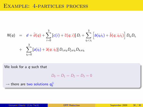
Example: 4-particles process
N(q) = d + d(q) +
3∑
i=0
[c(i) + c(q; i)]Di +
3∑
i0<i1
[
b(i0i1) + b(q; i0i1)]
Di0Di1
+
3∑
i0=0
[a(i0) + a(q; i0)] Di 6=i0Dj 6=i0Dk 6=i0
We look for a q such that
D0 = D1 = D2 = D3 = 0
→ there are two solutions q±0
Giovanni Ossola (City Tech) OPP Reduction September 2009 30 / 30
Page 36
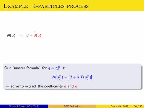
Example: 4-particles process
N(q) = d + d(q)
Our “master formula” for q = q±0 is:
N(q±0 ) = [d + d T (q±
0 )]
→ solve to extract the coefficients d and d
Giovanni Ossola (City Tech) OPP Reduction September 2009 30 / 30
Page 37
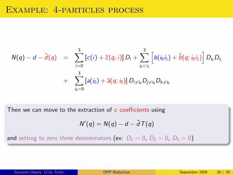
Example: 4-particles process
N(q) − d − d(q) =
3∑
i=0
[c(i) + c(q; i)]Di +
3∑
i0<i1
[
b(i0i1) + b(q; i0i1)]
Di0Di1
+
3∑
i0=0
[a(i0) + a(q; i0)] Di 6=i0Dj 6=i0Dk 6=i0
Then we can move to the extraction of c coefficients using
N ′(q) = N(q) − d − dT (q)
and setting to zero three denominators (ex: D1 = 0, D2 = 0, D3 = 0)
Giovanni Ossola (City Tech) OPP Reduction September 2009 30 / 30
Page 38
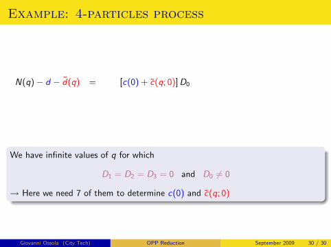
Example: 4-particles process
N(q) − d − d(q) = [c(0) + c(q; 0)]D0
We have infinite values of q for which
D1 = D2 = D3 = 0 and D0 6= 0
→ Here we need 7 of them to determine c(0) and c(q; 0)
Giovanni Ossola (City Tech) OPP Reduction September 2009 30 / 30