Mathematical Models and Methods in Applied Sciences Vol. 23, No. 13 (2013) 2523–2560 c World Scientific Publishing Company DOI: 10.1142/S0218202513500395 NUMERICAL HOMOGENIZATION OF A NONLINEARLY COUPLED ELLIPTIC–PARABOLIC SYSTEM, REDUCED BASIS METHOD, AND APPLICATION TO NUCLEAR WASTE STORAGE ANTOINE GLORIA D´ epartement de Math´ ematiques, Universit´ e Libre de Bruxelles (ULB), 1050 Brussels, Belgium and Project-team SIMPAF, Inria Lille–Nord Europe, 59650 Villeneuve d’Ascq, France [email protected]THIERRY GOUDON Project-team COFFEE, Inria Sophia Antipolis M´ editerran´ ee, France and Labo. J. A. Dieudonn´ e, UMR 7351, CNRS–Universit´ e Nice Sophia Antipolis, France [email protected]STELLA KRELL ANDRA DRD/EAP and Project-team SIMPAF, Inria Lille–Nord Europe, France (Current address: Labo. J. A. Dieudonn´ e, UMR 7351, CNRS–Universit´ e Nice Sophia Antipolis) [email protected]Received 7 March 2012 Revised 8 January 2013 Accepted 14 January 2013 Published 23 April 2013 Communicated by C. Conca We consider the homogenization of a coupled system of PDEs describing flows in het- erogeneous porous media. Due to the coupling, the effective coefficients always depend on the slow variable, even in the simple case when the porosity is periodic. Therefore the most important part of the computational time for the numerical simulation of such flows is dedicated to the determination of these coefficients. We propose a new numerical algorithm based on Reduced Basis techniques, which significantly improves the compu- tational performances. Keywords : Porous media; homogenization; reduced basis method. AMS Subject Classification: 35B27, 65M60, 65Z05, 76M50, 76M10 2523 Math. Models Methods Appl. Sci. 2013.23:2523-2560. Downloaded from www.worldscientific.com by UNIVERSITY OF MIAMI on 09/29/13. For personal use only.
We consider the homogenization of a coupled system of PDEs describing flows in het-erogeneous porous media. Due to the coupling, the effective coefficients always dependon the slow variable, even in the simple case when the porosity is periodic. Thereforethe most important part of the computational time for the numerical simulation of suchflows is dedicated to the determination of these coefficients. We propose a new numericalalgorithm based on Reduced Basis techniques, which significantly improves the compu-tational performances.
This work is concerned with the numerical treatment of a nonlinearly coupledelliptic–parabolic system of equations whose coefficients vary on a small scale.Resolving the finest scales induces a prohibitive numerical cost, both in termsof computational time and memory storage. Our goal consists in finding relevant“averaged” models, combined with efficient numerical methods. It turns out thatthe main part of the computational effort is precisely devoted to the evaluation ofthe coefficients of the effective equations which are obtained by homogenization. Weshall propose methods which lead to a considerable speed-up of this crucial step.
A strong motivation comes from the modeling of radionuclide transport innuclear waste storage devices. This yields a nonlinear system of parabolic equations,coupling the time-evolution of the radionuclide concentration C(t, x) (for the sake ofsimplicity we consider only one single species of radionuclides) to the velocity fieldU(t, x) of the water flow. The flow takes place in a complex porous medium madeof clay, limestone and marl — so that the physical properties vary a lot from placeto place. The modeling of radionuclide transport in disposal facilities of radioactivewaste therefore requires to deal with PDEs whose coefficients are heterogeneousat small scales. The realization of routine simulations should however rely on fastcomputations, which excludes the finest scales. Homogenization is the natural toolto derive effective models, which hopefully smooth out in a consistent way the smallscale features of the problem. In the case of the nonlinearly coupled system treatedhere, (periodic) homogenization alone is not enough to drastically reduce the com-putational cost, since a so-called cell-problem (which is itself an elliptic PDE) hasto be solved at each Gauss point of the computational domain — this could surprisethe expert: although diffusion coefficients are assumed to be periodic, and the equa-tions are linear, the nonlinear coupling condition makes the homogenized diffusionmatrix depend on the space variable. This is where the reduced basis (RB) methodcomes into the picture: these cell-problems can be viewed as a d-parameter (d beingthe space dimension) family of elliptic equations, which is an ideal setting for theRB method. A further practical issue is related to the dependence of the ellipticoperator upon the parameters, which is not affine (according to the terminology ofthe RB approach) and therefore requires a specific treatment.
The model under investigation here has been derived for the benchmark COU-PLEX, see Ref. 4. This benchmark is based on a set of simplified but realistic modelsfor the transport of radionuclides around a nuclear waste repository. It allows oneto evaluate the pros and cons of several numerical strategies that can be used inthis context. We wish to complete the benchmark by considering the correspondinghomogenization problem. Let us recall the model. We are interested in the evolu-tion in time and space of the concentration C of a species (pollutant, nuclear waste,etc.) in a saturated porous medium Ω, which is driven by reaction, transport anddiffusion:
Rφ∂tC −∇ · (D(U)∇C − UC) +RφλC = S. (1.1)
Mat
h. M
odel
s M
etho
ds A
ppl.
Sci.
2013
.23:
2523
-256
0. D
ownl
oade
d fr
om w
ww
.wor
ldsc
ient
ific
.com
by U
NIV
ER
SIT
Y O
F M
IAM
I on
09/
29/1
3. F
or p
erso
nal u
se o
nly.
September 2, 2013 10:33 WSPC/103-M3AS 1350039
Nonlinearly Coupled Elliptic–Parabolic System 2525
This equation involves the following quantities: the fluid velocity U , a nonlineardiffusion matrix field D(U), the porosity φ > 0, the species-dependent latencyretardation factor R > 0 and degradation coefficient λ = ln(2)
T (where T is thehalf-time of the species), and a source term S. The system is completed by initialand boundary conditions, which can be of Dirichlet, Neumann, or mixed type.Both the diffusion coefficients D(U) and transport term U ·∇C depend on the fluidvelocity, which is itself related to the hydrodynamic load (or piezoelectric height)Θ = p
ρg + z (z = xd ∈ R being the height coordinate), through the formula
U = −K∇Θ, (1.2)
where K is the heterogeneous permeability tensor of the porous medium. In thiswork, we focus on the simplest situation possible where the hydraulic regime isestablished and governed by a mere diffusion equation relating the charge to thestationary source flow q:
∇ · U = q. (1.3)
The diffusion coefficients satisfy D(U) = D0 + D(U), where D0 is a diffusionmatrix field and D(U) is given by
D(U) = α|U |I + βU ⊗ U
|U | , (1.4)
for some α, β ≥ 0. We shall write the COUPLEX system (1.1)–(1.4) in dimension-less form, and identify a small parameter 0 < ε 1, which is the ratio betweenthe typical period of the heterogeneities and the characteristic length scale of Ω.The rescaled system has the same form as (1.1)–(1.4), with however a permeabil-ity matrix of the form K(x/ε) for some periodic function K. We may consideroscillating source terms q, S and diffusion coefficient D0 as well.
This work addresses the following questions:
(1) prove existence and uniqueness of suitable weak solutions to the COUPLEXsystem (1.1)–(1.4),
(2) find effective equations for this model of transport of radionuclides in porousmedia describing the regime 0 < ε 1,
(3) design numerical methods to compute efficiently the coefficients of the effectivemodels, without using the brutal and prohibitive method consisting of solvingindependently the cell-problems and computing the suitable averages at eachGauss point of the computational domain.
The first two points are considered as a preliminary to the design of a numericalsolution method. Note that the COUPLEX system can be embedded into a muchmore general family of systems, which has been widely studied in the literature.The main difference with the existing literature is the coupling condition: in theCOUPLEX system (1.1)–(1.4), C depends on Θ but Θ does not depend on C; thisis a weak coupling. In more general models, Θ depends on C through an additional
Mat
h. M
odel
s M
etho
ds A
ppl.
Sci.
2013
.23:
2523
-256
0. D
ownl
oade
d fr
om w
ww
.wor
ldsc
ient
ific
.com
by U
NIV
ER
SIT
Y O
F M
IAM
I on
09/
29/1
3. F
or p
erso
nal u
se o
nly.
September 2, 2013 10:33 WSPC/103-M3AS 1350039
2526 A. Gloria, T. Goudon & S. Krell
viscosity term in the Darcy equation (1.3); this is a strong coupling. In the lattercase, existence results have been obtained in Refs. 16, 17 and 10. Uniqueness ofweak solutions has not been proved in general. This is a specific feature of theCOUPLEX system, which we shall address in Sec. 2. The problem is not trivial sincethe coefficients D(U) are unbounded unless ∇Θ is bounded (which does not holdin general). The system with strong coupling has been homogenized by Choquetand Sili in Ref. 11. We provide a much simpler proof in the case of weak coupling,which includes in addition the uniqueness property. As will be shown in Sec. 2, theeffective model in the regime ε→ 0 has the form
∇ · U∗ = q∗,
∂tC∗ −∇ · (D∗∇C∗ − U∗C∗) + λC∗ = S∗,
(1.5)
where the functions S∗, q∗ are determined by suitable “averages” of the oscillatingfunctions S, q, while the velocity field U∗ and the diffusion coefficient D∗ are givenby relations of the form
U∗ = U(K, q), D∗ = D(D0, U∗), (1.6)
for some nonlinear maps U and D. The core of this paper is the numerical approxi-mation of this homogenized system in Sec. 3. We shall see that the direct approachfor the computation of the effective coefficients, which consists in solving correctorequations at each Gauss point of Ω, remains prohibitive in terms of computationalcost. We then propose a numerical strategy based on the RB method (see Ref. 21and the references therein for elliptic equations, and Ref. 5 for an application tohomogenization). The guideline of the RB approach is the construction of a suitableGalerkin basis “adapted” to the parametrized set of equations. We present in detailthe application of the RB method to the COUPLEX system (1.1)–(1.4). Again, thefact that the diffusion coefficients are unbounded raises some interesting questions,this time not only for the analysis but also for the practical implementation of theRB method, and more specifically for the choice of the estimator. Numerical resultsdemonstrate the ability of the method to provide accurate results with a substantialspeed-up.
We shall make use of the following notation:
• R+ = [0,+∞);
• 0 < T <∞ is a final time;• d ≥ 1 denotes the space dimension;• Md(R) is the set of d× d real matrices, I is the identity matrix;• Ω is an open bounded Lipschitz domain of R
d;• For all p ∈ [1,∞] and s ∈ N, Lp(Ω) denotes the space of p-integrable functions
on Ω, W s,p(Ω) denotes the Sobolev space of p-integrable functions whose s-firstdistributional derivatives are p-integrable, W 1,p
0 (Ω) the closure in W 1,p(Ω) of thespace C∞
0 (Ω) of smooth functions compactly supported in Ω;• For p = 2, we denote the Hilbert spaces W 1,2(Ω) and W 1,2
0 (Ω) by H1(Ω) andH1
0 (Ω), respectively;
Mat
h. M
odel
s M
etho
ds A
ppl.
Sci.
2013
.23:
2523
-256
0. D
ownl
oade
d fr
om w
ww
.wor
ldsc
ient
ific
.com
by U
NIV
ER
SIT
Y O
F M
IAM
I on
09/
29/1
3. F
or p
erso
nal u
se o
nly.
September 2, 2013 10:33 WSPC/103-M3AS 1350039
Nonlinearly Coupled Elliptic–Parabolic System 2527
• Y = (0, 1)d is the periodic cell, and H1#(Y) denotes the closure of the subspace
of C∞(Rd) made of Y-periodic functions with vanishing mean.
2. Well-Posedness and Homogenization
2.1. Main results
Let λ > 0, q ∈ L∞(Ω), and S ∈ L2(0, T ;H−1(Ω)). We consider the following weaklycoupled system of PDEs:
U = −K∇Θ in Ω,
∇ · U = q in Ω,
∂tC −∇ · (D(U)∇C − UC) + λC = S in ]0, T [×Ω.
(2.1)
The weak coupling condition reads
D(U)(x) := D0(x) + α|U(x)|I + βU(x) ⊗ U(x)
|U(x)| , (2.2)
for a.e. x ∈ Ω, where α > 0, β ≥ 0. The functions x → K(x) and x → D0(x) arematrix-valued; they both satisfy uniform bounds and strong ellipticity conditions:there exists Λ > 0 such that for a.e. x ∈ Ω and all ξ ∈ R
The system (2.1) is complete by boundary conditions and an initial condition.For the mathematical analysis of the problem, we restrict ourselves to homogeneousDirichlet boundary conditions; namely, we set
Θ = 0 on ∂Ω,
C(0, ·) = Cinit in Ω,
C = 0 on ]0, T [×∂Ω,
(2.3)
for some Cinit ∈ L2(Ω). The adaptation to more general (time-independent) bound-ary conditions, as treated in the numerical tests later on, could be considered with-out further difficulty.
We are interested in the case when K is an ε-periodic matrix, and ε→ 0. Beforewe turn to this problem, we first define a notion of weak solution for the coupledsystem (2.1)–(2.3), and give an existence and uniqueness result.
Definition 1. A weak solution of (2.1)–(2.3) is a pair (Θ, C) ∈ H10 (Ω) × L2(0, T ;
H10 (Ω))∩C0(0, T ;L2(Ω)) such that ∂tC ∈ L2(0, T ;H−1(Ω)),
∫ T
0
∫Ω∇C ·D(U)∇C <
∞ with U = −K∇Θ, and which satisfies (2.1)–(2.3) in the following sense:
• Θ is a weak solution in H10 (Ω) to (2.1)1,2 and (2.3)1;
• For all v ∈ L2(0, T ;H10 (Ω))∩L2(0, T ;L∞(Ω)) such that
∫ T
0
∫Ω∇v ·D(U)∇v <∞,
Mat
h. M
odel
s M
etho
ds A
ppl.
Sci.
2013
.23:
2523
-256
0. D
ownl
oade
d fr
om w
ww
.wor
ldsc
ient
ific
.com
by U
NIV
ER
SIT
Y O
F M
IAM
I on
09/
29/1
3. F
or p
erso
nal u
se o
nly.
September 2, 2013 10:33 WSPC/103-M3AS 1350039
2528 A. Gloria, T. Goudon & S. Krell
we have ∫ T
0
〈∂tC, v〉H−1,H10
+∫ T
0
∫Ω
∇v ·D(U)∇C +∫ T
0
∫Ω
vU · ∇C
+∫ T
0
∫Ω
Cv(q + λ) =∫ T
0
〈S, v〉H−1,H10.
The following theorem states the existence and uniqueness of such weak solu-tions.
Theorem 1. For all q ∈ L∞(Ω), S ∈ L2(0, T ;H−1(Ω)) and Cinit ∈ L2(Ω), thereexists a unique weak solution to (2.1)–(2.3) in the sense of Definition 1.
We now turn to the periodic homogenization of (2.1)–(2.3). Let K be a Y =(0, 1)d-periodic matrix. For all ε > 0, we consider the coupled system
Uε = −Kε∇Θε in Ω,
∇ · Uε = q in Ω,
∂tCε −∇ · (D(Uε)∇Cε − UεCε) + λCε = S in ]0, T [×Ω,
Θε = 0 on ∂Ω,
Cε(0, ·) = Cinit in Ω,
Cε = 0 on ]0, T [×∂Ω,
(2.4)
where q, S, Cinit and the function D are as above, and Kε is defined by Kε(x) :=K(x/ε) on Ω. Theorem 1 ensures the existence and uniqueness of a weak solution(Θε, Cε) of (2.4) for all ε > 0. In order to characterize the asymptotic behaviorof (Θε, Cε) as ε → 0 we need to introduce a few auxiliary quantities. For all i ∈1, . . . , d, we let ϕi denote the unique periodic weak solution in H1
#(Y) to thefollowing elliptic equation
−∇ ·K(ei + ∇ϕi) = 0. (2.5)
We define the matrix K∗ by: for all i, j ∈ 1, . . . , d,
ej ·K∗ei =∫
Y
(ej + ∇ϕj) ·K(ei + ∇ϕi). (2.6)
The matrix K∗ defined this way is strongly elliptic. This allows one to define theunique weak solution Θ0 ∈ H1
0 (Ω) to the elliptic equation
−∇ ·K∗∇Θ0 = q. (2.7)
The homogenized drift is then given by
U0 = −K∗∇Θ0. (2.8)
Mat
h. M
odel
s M
etho
ds A
ppl.
Sci.
2013
.23:
2523
-256
0. D
ownl
oade
d fr
om w
ww
.wor
ldsc
ient
ific
.com
by U
NIV
ER
SIT
Y O
F M
IAM
I on
09/
29/1
3. F
or p
erso
nal u
se o
nly.
September 2, 2013 10:33 WSPC/103-M3AS 1350039
Nonlinearly Coupled Elliptic–Parabolic System 2529
Next we have to consider two-scale functions U , D defined on Ω × Y by
We point out that, while K∗ is a constant matrix, D∗ is not a constant matrix field,since ∇Θ0 is in general not constant on Ω. We are now in position to describe theasymptotic behavior.
Theorem 2. Let q ∈ L∞(Ω), S ∈ L2(0, T ;H−1(Ω)), Cinit ∈ L2(Ω), D be as in(2.2), and let K be a Y-periodic bounded and strongly elliptic matrix. For all ε > 0,we set Kε := K(·/ε). We let K∗, Θ0, U0 and D∗ be as in (2.6), (2.7), (2.8) and(2.11), respectively. Then there exists a unique weak solution C0 to
∂tC0 −∇ · (D∗∇C0 − U0C0) + λC0 = S in ]0, T [×Ω,
C0(0, ·) = Cinit in Ω,
C0 = 0 on ]0, T [×∂Ω,
(2.12)
in the sense of Definition 1 (with D∗ in place of D(U)), and the unique weaksolution (Θε, Cε) to (2.4) converges to (Θ0, C0) strongly in L2(Ω) and L2((0, T ) ×Ω), and weakly in H1(Ω) and L2(0, T ;H1(Ω)); in addition Cε converges inC0([0, T ], L2(Ω)-weak) to C0.
Although the diffusion D∗ is not of the form (2.2), for all x ∈ Ω, D∗(x) onlydepends on ∇Θ0(x), and D∗ ∈ L2(Ω). Hence existence and uniqueness of weaksolutions for the homogenized system can be proved the same way as for Theo-rem 1, and we leave the details to the reader. From the homogenization point ofview, Theorem 2 is a rather direct application of two-scale convergence and Theo-rem 1. Although D(U) is unbounded, it is square-integrable and the homogenizedsystem remains elliptic-parabolic (for the homogenization of elliptic equations withunbounded coefficients which are not equi-integrable, nonlocal effects may appear,
Mat
h. M
odel
s M
etho
ds A
ppl.
Sci.
2013
.23:
2523
-256
0. D
ownl
oade
d fr
om w
ww
.wor
ldsc
ient
ific
.com
by U
NIV
ER
SIT
Y O
F M
IAM
I on
09/
29/1
3. F
or p
erso
nal u
se o
nly.
September 2, 2013 10:33 WSPC/103-M3AS 1350039
2530 A. Gloria, T. Goudon & S. Krell
and we refer the reader to Refs. 2 and 6). In the case of strong coupling (thatis when the equation for U depends on C through a nonconstant viscosity term),homogenization has been proved in Ref. 11. Yet Ref. 11 is an overkill for the prob-lem under consideration (uniqueness is not discussed in Ref. 11 though), and wedisplay the main arguments of a simpler proof in Appendix A.
Remark 1. In this statement we have considered only the case of a periodic oscil-lating matrix K. Note that, even in this simple case, the matrix D depends onboth the slow variable x ∈ Ω and the fast variable y ∈ Y. The result generalizesreadily to the case of a locally periodic fields of the form K(x, x/ε). Similarly, oscil-lating source terms and diffusion coefficients D0, depending on x and x/ε, can beconsidered.
Since the specific feature of the coupled model under investigation is the unique-ness of weak solutions, we prove Theorem 1 in detail in the following subsection.
2.2. Proof of Theorem 1
The difference with respect to previous contributions on the strongly coupled systemis the fact that weak solutions can be proved to be unique for the weakly coupledsystem. The only subtle feature of the system is the integrability condition on D
and U , which are square-integrable but not necessarily essentially bounded. Theproof is based on standard regularization and compactness arguments. We shallonly prove the uniqueness of weak solutions in detail.
For the reader convenience we quickly sketch the proof of existence of weaksolutions as well. We divide the proof into six steps, and proceed by regularization.In the first step we recall a classical result essentially due to J.-L. Lions. In thesecond step we introduce the regularizations for U and D(U). In the third step weapply Step 1 and derive a priori estimates. In Step 4 we deduce from these a prioriestimates, by compactness and Aubin-Simon’s arguments, that the weakly coupledsystem admits a distributional solution. We then show in Step 5 that this solutionsatisfies a weak formulation of the equation. We prove uniqueness of weak solutionsin Step 6.
Step 1. Case of bounded coefficients and drifts.Let D : Ω → Md(R) be uniformly bounded and strongly elliptic, and U ∈L∞(Ω,Rd). We consider the equation
∂tC −∇ · (D∇C − UC) + λC = S in ]0, T [×Ω,
C(0, ·) = Cinit in Ω,
C = 0 on ]0, T [×∂Ω.
(2.13)
Then for all S ∈ L2(0, T ;H−1(Ω)) and Cinit ∈ L2(Ω) there exists a unique functionC ∈ L2(0, T ;H1
0(Ω)) ∩ C0(0, T ;L2(Ω)) such that ∂tC ∈ L2(0, T ;H−1(Ω)), which
Mat
h. M
odel
s M
etho
ds A
ppl.
Sci.
2013
.23:
2523
-256
0. D
ownl
oade
d fr
om w
ww
.wor
ldsc
ient
ific
.com
by U
NIV
ER
SIT
Y O
F M
IAM
I on
09/
29/1
3. F
or p
erso
nal u
se o
nly.
September 2, 2013 10:33 WSPC/103-M3AS 1350039
Nonlinearly Coupled Elliptic–Parabolic System 2531
satisfies the weak form of (2.13): for all v ∈ L2(0, T ;H10 (Ω)) and all T > 0,∫ T
0
〈∂tC, v〉H−1,H10
+∫ T
0
∫Ω
∇v ·D∇C −∫ T
0
∫Ω
CU · ∇v + λ
∫ T
0
∫Ω
Cv
=∫ T
0
〈S, v〉H−1,H10.
Note that by an exponential change of time, one may assume λ to be as largeas desired (which then ensures the coercivity of the bilinear form). We refer thereader to Ref. 23 for details. In the sequel we shall use the following equivalentweak formulation: for all v ∈ L2(0, T ;H1
0 (Ω)) and all t > 0,∫ t
0
〈∂tC, v〉H−1,H10
+∫ t
0
∫Ω
∇v ·D∇C +∫ t
0
∫Ω
∇C · Uv +∫ t
0
∫Ω
(q + λ)Cv
=∫ t
0
〈S, v〉H−1,H10, (2.14)
which we obtain by using the divergence theorem and the identity ∇ · U = q.
Step 2. Regularizations.First note that the elliptic part of the system
U = −K∇Θ in Ω,
∇ · U = q in Ω,
Θ = 0 on ∂Ω,
(2.15)
admits a unique weak solution Θ ∈ H10 (Ω). The associated drift U = −K∇Θ is
not essentially bounded, but square-integrable. Likewise the associated diffusioncoefficients D(U) are not essentially bounded, but square-integrable. In particular,the advection–diffusion equation
∂tC −∇ · (D(U)∇C − UC) + λC = S in ]0, T [×Ω,
C(0, ·) = Cinit in Ω,
C = 0 on ]0, T [×∂Ω,
(2.16)
does not satisfy the assumptions of Step 1. We regularize D(U) and U , and beginwith the diffusion coefficients. Since D(U) is a symmetric matrix, for a.e. x ∈ Ωthere exist α1(x), . . . , αd(x) ≥ 0, and a unitary matrix P (x) such that D(U)(x) =PT (x)diag(α1(x), . . . , αd(x))P (x). For all M > 0 and a.e. x ∈ Ω, we define DM (x)as follows:
In particular, DM converges monotonically to D(U) in L2(Ω) as M → ∞. Forthe regularization of U , we prefer to regularize the defining equation ∇ · U = q
rather than using truncations. We consider KM and qM two sequences of smoothfunctions such that KM and qM are bounded in L∞(Ω) and converge to K and q
Mat
h. M
odel
s M
etho
ds A
ppl.
Sci.
2013
.23:
2523
-256
0. D
ownl
oade
d fr
om w
ww
.wor
ldsc
ient
ific
.com
by U
NIV
ER
SIT
Y O
F M
IAM
I on
09/
29/1
3. F
or p
erso
nal u
se o
nly.
September 2, 2013 10:33 WSPC/103-M3AS 1350039
2532 A. Gloria, T. Goudon & S. Krell
in Lr(Ω) for all r <∞, respectively. We define ΘM as the unique weak solution inH1
0 (Ω) to
−∇ · (KM∇ΘM ) = qM
and set UM := −KM∇ΘM . By elliptic regularity, UM belongs to L∞(Ω). Further-more, UM converges to U in L2(Ω) (the argument relies on Meyers’ estimate, whichimplies that ∇ΘM converges to ∇Θ in Lp(Ω) for some p > 2 depending only onthe constant Λ, whereas KM converges in Lp′
(Ω) to K, with 1/p+ 1/p′ = 1).Hence, for all M > 0, Step 1 implies there exists a unique weak solution
CM ∈ L2(0, T ;H10(Ω)) ∩ C0(0, T ;L2(Ω)) such that ∂tC
M ∈ L2(0, T ;H−1(Ω)) tothe regularized equation
∂tCM −∇ · (DM∇CM − UMCM ) + λCM = S in ]0, T [×Ω,
CM (0, ·) = Cinit in Ω,
CM = 0 on ]0, T [×∂Ω.
(2.17)
It remains to pass to the limit as M → ∞.
Step 3. A priori estimates.The weak form of (2.17) with test-function CM itself yields for all 0 < t ≤ T ,∫ t
0
〈∂tCM , CM 〉H−1,H1
0+∫ t
0
∫Ω
∇CM ·DM∇CM −∫ t
0
∫Ω
CMUM · ∇CM
+λ
∫ t
0
∫Ω
(CM )2 =∫ t
0
〈S,CM 〉H−1,H10.
Since ∇ · UM = qM , we have by the divergence theorem
−∫ t
0
∫Ω
CMUM · ∇CM = −12
∫ t
0
∫Ω
UM · ∇(CM )2 =12
∫ t
0
∫Ω
q(CM )2,
so that the weak form turns into
12
∫Ω
(CM (·, t))2 +∫ t
0
∫Ω
∇CM ·DM∇CM +∫ t
0
∫Ω
(CM )2(
12qM + λ
)=
12
∫Ω
C2init +
∫ t
0
〈S,CM 〉H−1,H10.
Recalling that one may take λ such that 12 inf qM + λ ≥ − 1
2 supM‖qM‖L∞(Ω) +λ = λ∗ > 0, we finally deduce by coercivity of DM (and arbitrariness of t):
12
sup0<t≤T
∫Ω
(CM (·, t))2 + Λ−1‖∇CM‖2L2(0,T ;L2(Ω)) + λ∗‖CM‖2
L2(0,T ;L2(Ω))
≤ ‖S‖L2(0,T ;H−1(Ω))‖CM‖L2(0,T ;H10 (Ω)) +
12‖Cinit‖2
L2(Ω).
Using this estimate, Young’s inequality, and the equation again, we finally obtainthat CM is bounded in L2(0, T ;H1
0 (Ω)) ∩ L∞(0, T ;L2(Ω)) and that ∂tCM is
bounded in L2(0, T ;H−1(Ω)), uniformly in M .
Mat
h. M
odel
s M
etho
ds A
ppl.
Sci.
2013
.23:
2523
-256
0. D
ownl
oade
d fr
om w
ww
.wor
ldsc
ient
ific
.com
by U
NIV
ER
SIT
Y O
F M
IAM
I on
09/
29/1
3. F
or p
erso
nal u
se o
nly.
September 2, 2013 10:33 WSPC/103-M3AS 1350039
Nonlinearly Coupled Elliptic–Parabolic System 2533
Step 4. Compactness and existence of distributional solutions.By weak compactness and Aubin-Simon’s theorem (see Ref. 25), there exists afunction C ∈ L2(0, T ;H1
0(Ω)) ∩ C0(0, T ;L2(Ω)) with ∂tC ∈ L2(0, T ;H−1(Ω)) suchthat CM converges weakly to C in L2(0, T ;H1
0(Ω)), strongly in L2(0, T ;L2(Ω)),and such that ∂tC
M converges weakly to ∂tC in L2(0, T ;H−1(Ω)).It is easy to check that C solves (2.16) in the sense of distributions, and satisfies
the initial condition as a continuous function in time taking values in L2(Ω).
Step 5. Weak formulation of the system.In this step, we shall prove that (Θ, C) is a weak solution of (2.1)–(2.3) in the senseof Definition 1. We start by showing that
∫ T
0
∫Ω ∇C ·D(U)∇C < ∞, which is not
obvious a priori since ∇C ∈ L2(Ω) and D(U) ∈ L2(Ω). Let M ′ > 0 be fixed. Byweak lower-semicontinuity, since ∇CM converges weakly to ∇C in L2(0, T ;L2(Ω)),∫ T
0
∫Ω
∇C ·DM ′∇C ≤ lim infM→∞
∫ T
0
∫Ω
∇CM ·DM ′∇CM .
Since M → DM is an increasing function in the sense of symmetric matrices,the a priori estimate of Step 3 implies for all M ≥M ′,∫ T
0
∫Ω
∇CM ·DM ′∇CM ≤∫ T
0
∫Ω
∇CM ·DM∇CM
≤ ‖Cinit‖2L2(Ω) + ‖S‖2
L2(0,T ;H−1(Ω)).
Hence, ∫ T
0
∫Ω
∇C ·DM ′∇C ≤ ‖Cinit‖2L2(Ω) + ‖S‖2
L2(0,T ;H−1(Ω))
and the desired estimate∫ T
0
∫Ω
∇C ·D(U)∇C ≤ ‖Cinit‖2L2(Ω) + ‖S‖2
L2(0,T ;H−1(Ω)),
follows from the monotone convergence theorem as M ′ → ∞, using again themonotonicity of M → DM .
Let v ∈ L2(0, T ;H10 (Ω))∩L2(0, T ;L∞(Ω)) be such that
∫ T
0
∫Ω ∇v ·D(U)∇v <
∞. In order to prove that C is a weak solution, we need to pass to the limit asM → ∞ in the weak formulation (2.14) for CM , i.e.∫ t
0
〈∂tCM , v〉H−1,H1
0+∫ t
0
∫Ω
∇v ·DM∇CM +∫ t
0
∫Ω
∇CM · UMv
+∫ t
0
∫Ω
(q + λ)CMv =∫ t
0
〈S, v〉H−1,H10.
In view of the regularity of v, the convergence of UM to U in L2(Ω), and the weakcompactness of CM obtained in Step 4, the only nontrivial term to treat is thesecond-order term, and we shall prove that
limM→∞
∫ T
0
∫Ω
∇v ·DM∇CM =∫ T
0
∫Ω
∇v ·D(U)∇C.
Mat
h. M
odel
s M
etho
ds A
ppl.
Sci.
2013
.23:
2523
-256
0. D
ownl
oade
d fr
om w
ww
.wor
ldsc
ient
ific
.com
by U
NIV
ER
SIT
Y O
F M
IAM
I on
09/
29/1
3. F
or p
erso
nal u
se o
nly.
September 2, 2013 10:33 WSPC/103-M3AS 1350039
2534 A. Gloria, T. Goudon & S. Krell
Let M ′ > 0 be fixed. We rewrite the above term as∫ T
0
∫Ω
∇v ·DM∇CM
=∫ T
0
∫Ω
∇v · (DM −DM ′)∇CM +
∫ T
0
∫Ω
∇v ·DM ′∇CM . (2.18)
We focus on the second term of the R.H.S. and first take the limit as M → ∞.Since DM ′
is bounded, this yields
limM→∞
∫ T
0
∫Ω
∇v ·DM ′∇CM =∫ T
0
∫Ω
∇v ·DM ′∇C.
We conclude by the dominated convergence theorem that
limM ′→∞
limM→∞
∫ T
0
∫Ω
∇v ·DM ′∇CM =∫ T
0
∫Ω
∇v ·D(U)∇C,
since by Young’s inequality and monotonicity of M → DM ,
|∇v ·DM ′∇C| ≤ 12(∇v ·D(U)∇v + ∇C ·D(U)∇C),
which is integrable.It remains to prove that the first term of the R.H.S. of (2.18) vanishes as M ′ and
M go to infinity. By Cauchy–Schwarz inequality and monotonicity of M → DM ,we have∣∣∣∣∣
∫ T
0
∫Ω
∇v · (DM −DM ′)∇CM
∣∣∣∣∣≤(∫ T
0
∫Ω
∇v · (D −DM ′)∇v
)1/2(∫ T
0
∫Ω
∇CM ·DM∇CM
)1/2
.
The second factor of the R.H.S. is bounded by Step 3 uniformly in M . We thereforefocus on the first factor. Since D −DM ′ ≤ D in the sense of symmetric matricesand ∇v ·D∇v ∈ L1(Ω), the dominated convergence theorem yields
limM ′→∞
∫ T
0
∫Ω
∇v · (D −DM ′)∇v = 0
and therefore
limM ′→∞
lim supM→∞
∣∣∣∣∣∫ T
0
∫Ω
∇v · (DM −DM ′)∇CM
∣∣∣∣∣ = 0,
which concludes the proof of this step.
Step 6. Uniqueness of weak solutions.Since Eq. (2.16) is linear with respect to C, uniqueness follows formally from theweak formulation tested with the solution C itself. However, we cannot directlyproceed this way since C /∈ L2(0, T ;L∞(Ω)) a priori and it is not clear whether it
Mat
h. M
odel
s M
etho
ds A
ppl.
Sci.
2013
.23:
2523
-256
0. D
ownl
oade
d fr
om w
ww
.wor
ldsc
ient
ific
.com
by U
NIV
ER
SIT
Y O
F M
IAM
I on
09/
29/1
3. F
or p
erso
nal u
se o
nly.
September 2, 2013 10:33 WSPC/103-M3AS 1350039
Nonlinearly Coupled Elliptic–Parabolic System 2535
can be used as an admissible test function. Instead we use a standard truncationargument: for all N > 0 we define a function ϕN : R → R as
ϕN (x) :=
−N for x < −N,x for |x| ≤ N,
N for x > N
and we test the weak formulation of (2.16) with CN := ϕN (C) ∈ L2(0, T ;H10 (Ω))∩
L∞((0, T ) × Ω). This yields∫ T
0
〈∂tC,CN 〉H−1,H10
+∫ T
0
∫Ω
∇CN ·D(U)∇C +∫ T
0
∫Ω
CNU · ∇C
+∫ T
0
∫Ω
CCN (q + λ) =∫ T
0
〈S,CN 〉H−1,H10. (2.19)
It is easy to prove that CN → C in L2(0, T ;H1(Ω)) as N → ∞ so that wecan pass to the limit in the first and last terms of the L.H.S. and in the R.H.S. of(2.19). It remains to treat the last two terms. We begin with the Dirichlet form. Bydefinition of ϕN and CN ,
∇C ·D(U)∇C.We now turn to the third term of the L.H.S. of (2.19), which we treat together
with the term involving q. In particular since ∇ · U = q, the divergence theoremyields ∫ T
0
∫Ω
CNU · ∇C +∫ T
0
∫Ω
CCNq = −∫ T
0
∫Ω
CU · ∇CN .
Note that by definition of ϕN and CN we can rewrite this identity as∫ T
0
∫Ω
CNU · ∇C +∫ T
0
∫Ω
CCN q = −∫ T
0
∫Ω
CNU · ∇CN .
Using that ∇ · U = q and the divergence theorem again, this turns into∫ T
0
∫Ω
CNU · ∇C +∫ T
0
∫Ω
CCN q = −∫ T
0
∫Ω
CNU · ∇CN
= −12
∫ T
0
∫Ω
U · ∇C2N
=12
∫ T
0
∫Ω
qC2N .
Passing to the limit in the last identity yields
limN→∞
(∫ T
0
∫Ω
CNU · ∇C +∫ T
0
∫Ω
CCNq
)=
12
∫ T
0
∫Ω
qC2.
Mat
h. M
odel
s M
etho
ds A
ppl.
Sci.
2013
.23:
2523
-256
0. D
ownl
oade
d fr
om w
ww
.wor
ldsc
ient
ific
.com
by U
NIV
ER
SIT
Y O
F M
IAM
I on
09/
29/1
3. F
or p
erso
nal u
se o
nly.
September 2, 2013 10:33 WSPC/103-M3AS 1350039
2536 A. Gloria, T. Goudon & S. Krell
Gathering the results of this step, we obtain the following identity:
12
∫Ω
C2(T, ·) +∫ T
0
∫Ω
∇C ·D(U)∇C +∫ T
0
∫Ω
C2
(12q + λ
)
=∫ T
0
〈S,C〉H−1,H10
+12
∫Ω
C2init,
since∫ T
0 〈∂tC,C〉H−1,H10
= 12
∫Ω C
2(T, ·) − 12
∫ΩC
2(0, ·). This implies uniqueness ofweak solutions, and concludes the proof of Theorem 1.
3. Numerical Approximation of the Homogenized System
In this section we propose a numerical strategy to approximate the weak solutionto the homogenized system (2.7)–(2.12). There are essentially three steps to solve(2.7)–(2.12):
(1) The computation of K∗ and the approximation of Θ0. The latter is solution ofa standard elliptic equation once K∗ is known, see (2.7).
(2) The approximation of D∗(x) at every Gauss point x of Ω. This requires to solvea family of elliptic equations on the periodic cell Y, parametrized by the Gausspoints x via ∇Θ0(x).
(3) The numerical solution of the advection–diffusion equation (2.12).
As we shall see, the bottleneck of the numerical approximation of (2.7)–(2.12) interms of computational cost is the approximation of D∗ in the second step. A largepart of this section is dedicated to this problem, and we shall use a reduced basisapproach to drastically reduce this computational cost. We have chosen not to focuson the numerical strategy to solve the advection–diffusion equation (2.12) since theequation is rather “standard” once D∗ is known. In particular, for the numeri-cal tests of the coupled system we use a naive P1-finite element method in spacecombined with the implicit Euler method in time. For more efficient and modernmethods, we refer the reader to Refs. 24, 14, 15, 26, 27, 8 and 9. The main contri-bution of this section (a numerical method for the computation of D∗) can indeedbe combined with any strategy to solve the advection–diffusion equation (2.12).
In the first subsection we present a direct approach to solve (2.7)–(2.12), andcomplement the homogenization result of Theorem 2 by numerical tests showing therate of convergence of (Θε, Cε) towards (Θ0, C0). As expected, the computationaltime to approximateD∗ becomes rapidly prohibitive as the number of discretizationpoints increases. In the second subsection we turn to the RB method. We firstquickly recall the rationale of the approach, and discuss what can be expected interms of convergence. We then turn to the practical implementation of the method,propose an a posteriori estimator adapted to homogenization problems (but notlimited to the specific one treated here), and present an original and effective wayof fast-assembling of the RB matrix, which is the major difficulty encountered in
Mat
h. M
odel
s M
etho
ds A
ppl.
Sci.
2013
.23:
2523
-256
0. D
ownl
oade
d fr
om w
ww
.wor
ldsc
ient
ific
.com
by U
NIV
ER
SIT
Y O
F M
IAM
I on
09/
29/1
3. F
or p
erso
nal u
se o
nly.
September 2, 2013 10:33 WSPC/103-M3AS 1350039
Nonlinearly Coupled Elliptic–Parabolic System 2537
the RB method when the dependence of the diffusion matrix upon the parameteris not affine — as it is the case here.
Before we turn to the core of this section let us point out that, as the attentivereader may have already noticed, it is not clear a priori that the finite elementmethod converges since the diffusion matrix in (2.12) is unbounded. The methoddoes indeed converge to the expected solution. This property can be proved alongthe lines of the existence-uniqueness theory developed in Sec. 2.
3.1. Direct approach
3.1.1. Space and time discretizations
We discretize the homogenized problem (2.7)–(2.12) with a finite element methodin space and the implicit Euler scheme in time. Let TΩ,h0 and TY,h1 ,TY,h1
be regulartessellations of Ω and of Y, respectively, into d-simplices of meshsizes h0, h1, h1 > 0.We denote by Vk
Ω,h0the space of Pk finite elements associated with TΩ,h0 for k = 0
and 1 (for k = 1, we only consider functions which vanish on the boundary), andby V1
Y,h1,V1
Y,h1(respectively V0
Y,h1) the subspaces of H1
#(Y) (respectively L2(Y))made of P1-periodic (respectively P0) finite elements associated with TY,h1 ,TY,h1
.As quickly mentioned above, a natural strategy to solve (2.7)–(2.12) is as follows:
Algorithm 1. (1) Numerical approximation K∗h1
of K∗: compute for all k ∈1, . . . , d Galerkin approximations ϕh1
k of ϕk in V1Y,h1
defined by: For all ψ ∈ V1Y,h1∫
Y
∇ψ ·K(ek + ∇ϕh1k ) = 0. (3.1)
Define then for all k, l ∈ 1, . . . , d,
el ·K∗h1
ek =∫
Y
(el + ∇ϕh1l ) ·K(ek + ∇ϕh1
k ).
For future reference, we set ϕh1 = (ϕh11 , . . . , ϕ
h1d ) ∈ H1
#(Y,Rd).
(2) Compute the Galerkin approximation Θh00 ∈ V1
Ω,h0of the solution to (2.7) with
K∗h1
in place of K∗, unique solution in V1Ω,h0
to: for all w ∈ V1Ω,h0
,∫Ω
∇w ·K∗h1∇Θh0
0 =∫
Ω
qw.
It defines Uh00 = −K∗
h1∇Θh0
0 , too.
(3) Approximation D∗h0
∈ V0Ω,h0
(each entry of the matrix is piecewise constant onTΩ,h0) of the homogenized diffusion D∗. Let ΠV0
Ω,h0denote the L2-projection onto
V0Ω,h0
. For every element T of the tessellation TΩ,h0 , ∇Θh00 |T is constant, and we
Mat
h. M
odel
s M
etho
ds A
ppl.
Sci.
2013
.23:
2523
-256
0. D
ownl
oade
d fr
om w
ww
.wor
ldsc
ient
ific
.com
by U
NIV
ER
SIT
Y O
F M
IAM
I on
09/
29/1
3. F
or p
erso
nal u
se o
nly.
September 2, 2013 10:33 WSPC/103-M3AS 1350039
2538 A. Gloria, T. Goudon & S. Krell
define D∗h0|T as follows: for all k, l ∈ 1, . . . , d,
el ·D∗h0|T ek =
∫Y
(el + ∇Φh1l |T ) · Dh1 |T (ek + ∇Φh1
k |T ),
where
Dh1 |T (y) := ΠV0Ω,h0
D0|T + D(Uh1 |T (y)),
Uh1 |T (y) := −K(y)(I + ∇ϕh1(y))∇Θh00 |T
and Φh1k |T ∈ V1
Y,h1is the unique periodic weak solution to: for all Ψ ∈ V1
Y,h1,∫
Y
∇Ψ · Dh1 |T (ek + ∇Φh1k |T ) = 0. (3.2)
(4) Approximation of C0. Let N ∈ N∗. The time interval [0, T ] is uniformly dis-
cretized with a fixed time step ∆t = TN . For all n ∈ 0, . . . , N, we set tn = n∆t,
and define the approximation Ch0,n0 ∈ V1
Ω,h0of C0(tn, ·) by induction as the unique
solution to: for all v ∈ V1Ω,h0
,∫Ω
Ch0,n+10 − Ch0,n
0
∆t+∫
Ω
∇v · (D∗h0∇Ch0,n+1
0 − Uh00 Ch0,n+1
0 )
+∫
Ω
λCh0,n+10 v =
∫Ω
Sn+1v.
Since we use an implicit time discretization, there is no CFL condition — note thatwe could have used a semi-implicit scheme as well (see for instance Ref. 23).
In this algorithm we have used two different discretizations V1Y,h1
and V1Y,h1
ofH1
#(Y). Indeed, Eq. (3.2) is an elliptic equation whose diffusion coefficients varya priori at scale h1, and it is reasonable to approximate its solutions with a finerdiscretization parameter h1 ≤ h1.
3.1.2. Numerical tests
To illustrate Theorem 2 when the homogenized system is solved using the directapproach of Algorithm 1, we consider a numerical test suggested by ANDRA.a Wetake d = 2 and let Ω = ]0, 2[2 be a square domain, and [0, T ] be the time intervalwith T = 1. The permeability is defined on the domain Y = ]0, 1[2 by:
∀ y = (y1, y2) ∈ Y, ∀ y1 ∈ ]0, 1[, K(y1, y2) =
4.94064, if y2 ≥ 0.5,
0.57816, if y2 < 0.5.
aAgence nationale pour la gestion des dechets radioactifs — http://www.andra.fr
Mat
h. M
odel
s M
etho
ds A
ppl.
Sci.
2013
.23:
2523
-256
0. D
ownl
oade
d fr
om w
ww
.wor
ldsc
ient
ific
.com
by U
NIV
ER
SIT
Y O
F M
IAM
I on
09/
29/1
3. F
or p
erso
nal u
se o
nly.
September 2, 2013 10:33 WSPC/103-M3AS 1350039
Nonlinearly Coupled Elliptic–Parabolic System 2539
Fig. 1. Laminate structure.
It has a laminate structure (see Fig. 1). We consider boundary conditions whichare slightly different from those in Theorem 2 and Algorithm 1 — note that theadaptations are straightforward in both cases:
Dirichlet boundary conditions: Let x = (x1, x2) ∈ ∂Ω.
The parameters used in the numerical tests are gathered in Table 1. As a con-sequence of the laminate structure, the correctors ϕ1 and ϕ2 and Φ1 and Φ2 belongto the finite element space V1
Y,h1provided the geometry of TY,h1 matches the lam-
inate structure of Fig. 1. In this case, one can therefore take h1 = h1. In Table 2we compare the approximations (Θεh1
system (2.7)–(2.12), for several values of ε (the discretization parameters h1 and h0
being fixed). The periodic cell Y is discretized with eight elements per dimension,and the macroscopic domain Ω is discretized using 2× 8/ε elements per dimensionto compute (Θεh1
ε , Cεh1ε ). For the approximation of (Θh0
0 , Ch00 ), we take h0 = 1/100.
This yields
• V1Y,h1
has dimension 81;• V1
Ω,h0has dimension ∼40,000;
• V1Ω,h0,ε has dimension ∼256ε−2.
We display in Table 2 the L2(Ω) norm of the error Θh00 − Θεh1
ε and theL2(Ω× ]0, T [)-norm of the error Ch0
0 −Ch1ε for ε ∈ 0.2, 0.1, 0.05, 0.025, that is, we
compare solutions of the homogenized problems to approximations of the solutionresolving the ε-scale (the case ε = 0.025 is already borderline in terms of computa-tional cost). These results have been obtained using FreeFem++ (see Ref. 19). Thelinear systems are solved with a direct solver. We obtain a first order of convergencefor both errors.
As can be seen in Table 2 the apparent convergence rates are of order 1, whichis consistent with a formal two-scale expansion, and shows the interest of replacing(Θε, Cε) by its homogenized counterpart (h0, C0). Although the computational timefor the approximation of (Θ0, C0) is much smaller than the computational timefor the approximation of (Θε, Cε) when ε is small, this method rapidly becomesprohibitive when the tessellation of Y gets finer since the approximation of D∗ thenbecomes quite expensive.
The last part of this paper is devoted to the speed up of the approximation ofD∗, with a numerical cost which should ideally be independent of the meshsize h1
of TY,h1 . From now on we assume D in (2.10) to be a symmetric matrix (that is,we assume D0 to be symmetric).
3.2. Reduced basis method for homogenization problems
In this section we describe how to apply the reduced basis method to the homog-enized problem under consideration, assuming in addition that D0 in (2.2) is aconstant matrix.
3.2.1. General presentation
The reduced basis method was introduced for the accurate online evaluation of(outputs of) solutions to a parameter-dependent family of elliptic PDEs. The basisof the method and further references can be found in Ref. 21. The applicationto the homogenization of elliptic equations is discussed in Ref. 5. Abstractly, itcan be viewed as a method to determine a “good” N -dimensional space SN to beused in approximating the elements of a set F = (Φ1(ξ), . . . ,Φd(ξ)), ξ ∈ P of
Mat
h. M
odel
s M
etho
ds A
ppl.
Sci.
2013
.23:
2523
-256
0. D
ownl
oade
d fr
om w
ww
.wor
ldsc
ient
ific
.com
by U
NIV
ER
SIT
Y O
F M
IAM
I on
09/
29/1
3. F
or p
erso
nal u
se o
nly.
September 2, 2013 10:33 WSPC/103-M3AS 1350039
Nonlinearly Coupled Elliptic–Parabolic System 2541
parametrized elements lying in a Hilbert space S, the parameter ξ ranging a certainsubset P ⊂ R
n.Let us describe how the computation of the effective coefficients we are con-
cerned with belongs to such a framework. First of all, the auxiliary function Θ0 issimply determined by solving the problem (2.7), with effective coefficients obtainedby solving the cell equations (2.5). There is no difficulty in this step and ∇xΘ0 canbe considered as given in this discussion. Then, we write the effective coefficient(2.10) for the concentration equation (2.12) as follows:
D(x, y) = D(∇xΘ0(x))(y),
where ξ ∈ Rd → D(ξ) ∈ L∞(Y,Md(R)) is defined by
D(ξ)(y) = D0 + α|M(y)ξ|I + βM(y)ξ ⊗M(y)ξ
|M(y)ξ| = D0 + D(M(y)ξ),
M(y) = K(y)(I + ∇ϕ(y)),
ϕ = (ϕ1, . . . , ϕd) solutions of (2.5).
(3.4)
We recall that α, β ≥ 0, and D0 is a positive-definite symmetric matrix whileM : Y → Md(R) is a square-integrable function. We are interested in the solutionΦk(ξ) ∈ H1
#(Y) to the problem: for all Ψ ∈ H1#(Y),∫
Y
∇Ψ(y) · D(ξ)(y)(ek + ∇Φk(ξ)(y)) dy = 0.
In the present context, S = H1#(Y) and we wish to find a convenient finite-
dimensional approximation space SN which allows one to describe the set F ofsolutions. In the rest of this section we particularize the standard RB method tohomogenization problems, by choosing a specific error estimator and orthogonal-ization procedure. To avoid further heavy notation, we do not display the variabley in what follows.
Let n ≥ 1 and let D : Rn → L∞(Y,Md(R)) be a function taking values in a set
of (y ∈ Y)-dependent d×d symmetric real matrices, satisfying uniform bounds andelliptic estimates. We suppose that D(ξ) depends continuously on the parameterξ ∈ R
n. Given a compact subset K of Rn, we set FK = (Φ1(ξ), . . . ,Φd(ξ)), ξ ∈ K,
where Φk(ξ) ∈ H1#(Y) denotes the unique periodic weak solution to the problem:
for all Ψ ∈ H1#(Y), and for all k ∈ 1, . . . , d,∫
Y
∇Ψ(ξ) · D(ξ)(ek + ∇Φk(ξ)) = 0.
The set FK is therefore compact in H1#(Y).
To construct the N -finite-dimensional space SN intended to approximate FK,we proceed by induction using a greedy algorithm. To this aim we need a reli-able estimator which measures the error between Φk(ξ) for some ξ ∈ K and its
Mat
h. M
odel
s M
etho
ds A
ppl.
Sci.
2013
.23:
2523
-256
0. D
ownl
oade
d fr
om w
ww
.wor
ldsc
ient
ific
.com
by U
NIV
ER
SIT
Y O
F M
IAM
I on
09/
29/1
3. F
or p
erso
nal u
se o
nly.
September 2, 2013 10:33 WSPC/103-M3AS 1350039
2542 A. Gloria, T. Goudon & S. Krell
approximation Φj
k(ξ) in Sj for 0 ≤ j ≤ N , which is defined as the unique weaksolution Φ
j
k(ξ) ∈ Sj to: for all Ψj ∈ Sj ,∫
Y
∇Ψj(ξ) · D(ξ)(ek + ∇Φ
j
k(ξ)) = 0. (3.5)
Recalling that we are dealing with a homogenization problem, the quantity of inter-est is the symmetric homogenized matrix D∗(ξ) defined for all k, l ∈ 1, . . . , d by(see (2.11))
el ·D∗(ξ)ek =∫
Y
(el + ∇Φl(ξ)) · D(ξ)(ek + ∇Φk(ξ)).
We denote by D∗,j(ξ) the approximation of D∗(ξ) using Sj , that is for all k, l ∈1, . . . , d
el ·D∗,j(ξ)ek =∫
Y
(el + ∇Φj
l (ξ)) · D(ξ)(ek + ∇Φj
k(ξ)).
A standard calculation using (3.5) and the symmetry of D yields
el · (D∗(ξ) −D∗,j(ξ))ek =∫
Y
(∇Φl(ξ) −∇Φj
l (ξ)) · D(ξ)(∇Φk(ξ) −∇Φj
k(ξ)).
This shows that the error on the homogenized matrix is a suitable estimator ofthe error at the level of the Φk. We thus define the estimator E
j:K×1, . . . , d →
R+ by
Ej(ξ, k) =
√|ek · (D∗(ξ) −D∗,j(ξ))ek|
ek ·D∗(ξ)ek
.
So defined, and recalling that D is assumed to take values in the set of uniformlyelliptic symmetric matrices (say with ellipticity constants 0 < ν ≤ ν < ∞), theestimator is such that there exist C1, C2 > 0 verifying for all suitable j, k, ξ theinequality
C1Ej(ξ, k) ≤ ‖∇Φk(ξ) −∇Φ
j
k(ξ)‖L2(Y) ≤ C2Ej(ξ, k). (3.6)
The induction procedure is then as follows. For all j ∈ 0, . . . , N − 1, chooseξj+1 ∈ K and kj+1 ∈ 1, . . . , d such that
(ξj+1, kj+1) = arg maxK,1,...,d
Ej,
define
Ψj+1 =Φkj+1(ξj+1) − Φ
j
kj+1(ξj+1)
‖∇Φkj+1(ξj+1) −∇Φj
kj+1(ξj+1)‖L2(Y)
and set
Sj+1 := span Ψ1, . . . ,Ψj+1.
Mat
h. M
odel
s M
etho
ds A
ppl.
Sci.
2013
.23:
2523
-256
0. D
ownl
oade
d fr
om w
ww
.wor
ldsc
ient
ific
.com
by U
NIV
ER
SIT
Y O
F M
IAM
I on
09/
29/1
3. F
or p
erso
nal u
se o
nly.
September 2, 2013 10:33 WSPC/103-M3AS 1350039
Nonlinearly Coupled Elliptic–Parabolic System 2543
By induction, for all j ∈ 0, . . . , N, dimSj+1 = j + 1, since by constructionΨj+1 is orthogonal to Sj for the following scalar product of H1
#(Y)
(Ψ1,Ψ2) →∫
Y
∇Ψ1 · D(ξj+1)∇Ψ2. (3.7)
Note that usually, in the RB literature, the vectors Ψj are orthogonalized using thesame scalar product for all j (whereas here, the scalar product depends on j).The choice made here makes the computation of the reduced basis simpler (andthe generated space Sj+1 is the same). The influence of this choice in practice isinvestigated numerically in Sec. 3.3.3.
What convergence rate can be expected in terms of N? In the case when n = 1and D has a dependence of the form D(ξ) = D0 + ξD1 (that is D is an affinefunction on the real line, and K is just a segment), the combination of results fromRef. 21 (and also the more general case treated in Ref. 12) and of Ref. 3 (see alsoRef. 7) shows that there exist c, C > 0 such that for all N ≥ 1,
supK,1,...,d
EN ≤ C exp(−cN).
The convergence being exponential in N , the reduced basis method is expected toyield accurate results for moderate N (say for N which is much smaller than thedimension of the finite element space V1
Y,h1for instance). Note that this yields a
complete control of the error on the homogenized coefficients since for all k, l ∈1, . . . , d by Cauchy–Schwarz’s inequality and definition of the estimator,
|el · (D∗(ξ) −D∗,N (ξ))ek| =∣∣∣∣∫
Y
(∇Φl(ξ) −∇ΦNl (ξ)) · D(ξ)(∇Φk(ξ) −∇ΦN
k (ξ))∣∣∣∣
≤√
(el ·D∗(ξ)el)(ek ·D∗(ξ)ek)EN(ξ, k)EN (ξ, l)
≤ C exp(−2cN),
for some constant C depending only on C and d, ν, ν.In the case under consideration here, D is replaced by D defined in (3.4). Things
are more complex than in Refs. 21 and 3 for the following three reasons:
• the parameter ξ is in Rd (i.e. n = d > 1 in the case of interest);
• a priori K = Rd, which is not a compact set;
• the function ξ → D(ξ) is nonlinear.
More generally, our working plan faces the following technical difficulties:
• The parameter ξ ranges over the whole Rd while the method is designed to deal
with parameters lying in a compact set.• The method simplifies significantly when the dependence of D upon ξ is affine.
In such a case it is described and analyzed in full details, whereas here thedependence with respect to the parameter is more intricate. The implementationof the method will require additional devices.
Mat
h. M
odel
s M
etho
ds A
ppl.
Sci.
2013
.23:
2523
-256
0. D
ownl
oade
d fr
om w
ww
.wor
ldsc
ient
ific
.com
by U
NIV
ER
SIT
Y O
F M
IAM
I on
09/
29/1
3. F
or p
erso
nal u
se o
nly.
September 2, 2013 10:33 WSPC/103-M3AS 1350039
2544 A. Gloria, T. Goudon & S. Krell
• The matrix M arising in the definition (3.4) of D is not essentially bounded asa function of y ∈ Y, but square-integrable only. Therefore the available resultsthat could be used to analyze the method simply do not apply.
The algorithm described in this paragraph is not of any practical use yet sincein order to choose ξj+1 and kj+1, one needs to know E
j(ξ, k) for all ξ and k. In the
following paragraph we describe the standard way to proceed in practice.
3.2.2. Practical reduced basis method
In practice we do not have access to Ej(ξ, k), ξ ∈ K, k ∈ 1, . . . , k since:
• the corrector Φk(ξ) has to be approximated in a finite-dimensional subspace Vof H1
#(Y), so that Ej
is approximated by some Ej ,• the space K has to be replaced by some finite set K.
The construction of the reduced basis is then as follows.
Algorithm 2. Let N ∈ N, p ≥ N , K = ξm, m ∈ 1, . . . , p be a finite subset ofK, and V be a finite-dimensional subspace of H1
#(Y).
(1) For all m ∈ 1, . . . , p and k ∈ 1, . . . , d, let Φk(ξm) ∈ V be an approximationof the corrector Φk(ξm) in V , that is the unique element of V such that for allΨ ∈ V , ∫
Y
∇Ψ · D(ξm)(ek + ∇Φk(ξm)) = 0
and let D∗kk(ξm) be the approximation of ek ·D∗(ξm)ek given by
D∗kk(ξm) =
∫Y
(ek + ∇Φk(ξm)) · D(ξm)(ek + ∇Φk(ξm)).
(2) Set V0 = 0.(3) While 0 ≤ j < N :
(a) For all m ∈ 1, . . . , p and k ∈ 1, . . . , d, let Φjk(ξm) ∈ V be an approxi-
mation of the corrector Φk(ξm) in Vj , that is the unique element of Vj suchthat for all Ψj ∈ Vj∫
Y
∇Ψj · D(ξm)(ek + ∇Φjk(ξm)) = 0
and let D∗,jkk (ξm) be the approximation of D∗
kk(ξm) given by
D∗,jkk (ξm) =
∫Y
(ek + ∇Φjk(ξm)) · D(ξm)(ek + ∇Φj
k(ξm)).
Mat
h. M
odel
s M
etho
ds A
ppl.
Sci.
2013
.23:
2523
-256
0. D
ownl
oade
d fr
om w
ww
.wor
ldsc
ient
ific
.com
by U
NIV
ER
SIT
Y O
F M
IAM
I on
09/
29/1
3. F
or p
erso
nal u
se o
nly.
September 2, 2013 10:33 WSPC/103-M3AS 1350039
Nonlinearly Coupled Elliptic–Parabolic System 2545
(b) For all m ∈ 1, . . . , p and k ∈ 1, . . . , d, define the estimator Ej(m, k) as
Ej(m, k) =
√|ek ·D∗(ξm)ek −D∗,j
kk (ξm)|ek ·D∗(ξm)ek
and set
(mj , kj) = arg maxK,1,...,d
Ej(m, k).
(c) Define
Ψj+1 :=Φkj (ξm) − Φj
kj(ξm)
‖∇Φkj (ξm) −∇Φjkj
(ξm)‖L2(Y)
and set
Vj+1 = span Ψi, 1 ≤ i ≤ j + 1.(d) j = j + 1.
Provided p is chosen large enough and V has dimension larger than N , one hasas in the previous paragraph dimVN = N .
What convergence rate can be expected in terms of N? Going back to theexample mentioned in the previous paragraph, that is for D(ξ) = D0+ξD1 and K asegment, the answer is given in Ref. 3. In particular it is proved that the exponentialestimate is stable in the sense that if the reduced basis VN is constructed startingfrom approximations of the correctors Φk(ξ), ξ ∈ K, k ∈ 1, . . . , d within anerror e, then the error estimate is of the form
supK,1,...,d
EN ≤ C exp(−cN) + Ce.
In Algorithm 2 there are two origins for the error e:
• The fact that H1#(Y) is replaced by a finite-dimensional space V , so that for all
ξ ∈ K and k ∈ 1, . . . , d, Φk(ξ) is a finite-dimensional approximation of Φk.• The fact that for the greedy algorithm, the argmax of the estimator is taken inK and not in K.
The first source of error is standard and can be controlled by a priori or aposteriori estimates. In the affine case above, the second source of error can alsobe estimated. Indeed, as proved in Ref. 13, the maps Φk : K → H1
#(Y), ξ →Φk(ξ) are analytic for all k ∈ 1, . . . , d. In particular, if K is a sampling of Kwith “meshsize” h, for all ξ ∈ K, Φk(ξ) can be approximated by interpolation inΦk(ξm), m ∈ 1, . . . , p within an error of order hq for any q ∈ N. Hence thepractical reduced basis method remains efficient in this specific case. However, thisanalysis is restricted to the affine case and it does not apply in our context.
Mat
h. M
odel
s M
etho
ds A
ppl.
Sci.
2013
.23:
2523
-256
0. D
ownl
oade
d fr
om w
ww
.wor
ldsc
ient
ific
.com
by U
NIV
ER
SIT
Y O
F M
IAM
I on
09/
29/1
3. F
or p
erso
nal u
se o
nly.
September 2, 2013 10:33 WSPC/103-M3AS 1350039
2546 A. Gloria, T. Goudon & S. Krell
3.2.3. Fast-assemby of the matrix
Let K, K and N ∈ N and VN be as in Algorithm 2. For all ξ ∈ K and k ∈ 1, . . . , d,the approximation of Φk(ξ) in the reduced basis VN is given by the unique functionΦN
k (ξ) ∈ VN such that for all ΨN ∈ VN ,∫Y
∇ΨN · D(ξ)(ek + ∇ΦNk (ξ)) = 0. (3.8)
Expanding ΦNk (ξ) in the basis VN as ΦN
k (ξ) =∑N
j=1 uj(ξ)Ψj , the above equationis equivalent to the linear system
M(ξ)U = B(ξ, k),
where for all j ∈ 1, . . . , N, Uj = uj(ξ) and B(ξ, k)j = −∫Y∇Ψj ·D(ξ)ek, and the
N × N matrix M(ξ) is given by its entries M(ξ)j1j2 =∫
Y∇Ψj1 · D(ξ)∇Ψj2 for all
1 ≤ j1, j2 ≤ N . In particular, in order to compute ΦNk (ξ), one needs to solve (3.8),
and therefore construct the matrix M(ξ) and the R.H.S. B(ξ, k).Without further assumptions on the function ξ → D(ξ), the exact calculation
of M(ξ) and B(ξ, k) requires:
• the storage of the coordinates of each vector Ψj of the reduced basis VN in thefinite-dimensional space V ;
• the computation of integrals over Y.
Both the information to be stored and the computational cost to construct M(ξ)and B(ξ, k) scale like the dimension dim(V) of the finite-dimensional space V (whichcan be prohibitively large). Yet, if ξ → D(ξ) has specific structural properties, theinformation to be stored and the computational cost can be drastically reduced.This is the case when ξ → D(ξ) is affine. Let us go back to the example of D(ξ) =D0 + ξD1. Then, the entries of the matrix M(ξ) and of the R.H.S. B(ξ, j) take theform: for all 1 ≤ j, j1, j2 ≤ N ,
M(ξ)j1j2 =∫
Y
∇Ψj1 ·D0∇Ψj2 + ξ
∫Y
∇Ψj1 ·D1∇Ψj2 ,
B(ξ, k)j =∫
Y
∇Ψj ·D0ek + ξ
∫Y
∇Ψj ·D1ek.
In particular, provided we store the following two N ×N matrices M1 and M2,and the following two d×N matrices B1 and B2 defined by: for all 1 ≤ j, j1, j2 ≤ N
and k ∈ 1, . . . , d,
(M1)j1j2 =∫
Y
∇Ψj1 ·D0∇Ψj2 , (M2)j1j2 =∫
Y
∇Ψj1 ·D1∇Ψj2 ,
(B1)kj =∫
Y
∇Ψj ·D0ek, (B2)kj =∫
Y
∇Ψj ·D1ek,
Mat
h. M
odel
s M
etho
ds A
ppl.
Sci.
2013
.23:
2523
-256
0. D
ownl
oade
d fr
om w
ww
.wor
ldsc
ient
ific
.com
by U
NIV
ER
SIT
Y O
F M
IAM
I on
09/
29/1
3. F
or p
erso
nal u
se o
nly.
September 2, 2013 10:33 WSPC/103-M3AS 1350039
Nonlinearly Coupled Elliptic–Parabolic System 2547
one may reconstruct M(ξ) and B(ξ, k) by the simple formulas
M(ξ) = M1 + ξM2, B(ξ, k) = (B1)k + ξ(B2)k,
where (B1)k and (B2)k are the kth column of B1 and B2, respectively.The gain is twofold:
• the dimension of the information to store is 2N2 + 2dN , which is independent ofdim(V);
• the computation of M(ξ) and B(ξ, k) only requires N2 +N multiplications andN2 +N additions, and not the computation of N2 +N integrals on Y (using anintegration rule which should be exact for functions of V).
The same strategy allows one to easily compute the approximation D∗,N(ξ) ofthe homogenized matrix D∗(ξ), via the formula: for all k, l ∈ 1, . . . , d,
ek ·D∗,N(ξ)el =∫
Y
(ek + ∇ΦNk (ξ)) · D(ξ)(el + ∇ΦN
l (ξ))
= ek
(∫Y
D0 + ξ
∫Y
D1
)el
+N∑
j=1
uj(ξ)ek ·(∫
Y
D0∇Ψj + ξ
∫Y
D1∇Ψj
),
so that one has to store 2d2+2dN real numbers only, to compute the approximationof the homogenized matrix.
This fast-assembly method is very convenient and efficient, but requires thediffusion matrix D(ξ) to be affine with respect to ξ.
3.3. Application of the reduced basis method to the
homogenized system
As said above, the evaluation of the effective coefficients for the homogenized prob-lem involves the parametrized matrices D defined in (3.4) where the parameterξ ranges the unbounded set R
d. In the following paragraph we shall rewrite theproblem in an equivalent form which allows one to work with a compact set ofparameters. We address the issue of fast assembly in the second paragraph, bearingin mind that the dependence with respect to the parameter is not affine. We providewith a numerical study of the method in the last paragraph.
3.3.1. Rewriting of the problem
The starting point to rewrite the problem is the following observation: for all ξ ∈ Rd
and all k ∈ 1, . . . , d, the corrector Φk(ξ) ∈ H1#(Y) is solution to
−∇ · D(ξ)1 + |ξ| (ek + ∇Φk(ξ)) = 0. (3.9)
Mat
h. M
odel
s M
etho
ds A
ppl.
Sci.
2013
.23:
2523
-256
0. D
ownl
oade
d fr
om w
ww
.wor
ldsc
ient
ific
.com
by U
NIV
ER
SIT
Y O
F M
IAM
I on
09/
29/1
3. F
or p
erso
nal u
se o
nly.
September 2, 2013 10:33 WSPC/103-M3AS 1350039
2548 A. Gloria, T. Goudon & S. Krell
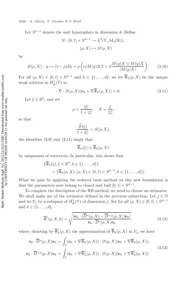
Let Sd−1 denote the unit hypersphere in dimension d. Define
D : [0, 1]× Sd−1 → L2(Y,Md(R)),
(ρ,X) → D(ρ,X)
by
D(ρ,X) : y → (1 − ρ)D0 + ρ
(α|M(y)X |I + β
M(y)X ⊗M(y)X|M(y)X |
). (3.10)
For all (ρ,X) ∈ [0, 1] × Sd−1 and k ∈ 1, . . . , d, we let Φk(ρ,X) be the uniqueweak solution in H1
#(Y) to
−∇ · D(ρ,X)(ek + ∇Φk(ρ,X)) = 0. (3.11)
Let ξ ∈ Rd, and set
ρ =|ξ|
1 + |ξ| , X =ξ
|ξ| ,
so that
D(ξ)1 + |ξ| = D(ρ,X),
the identities (3.9) and (3.11) imply that
Φk(ξ) ≡ Φk(ρ,X)
by uniqueness of correctors. In particular, this shows that
Φk(ξ), ξ ∈ Rd, k ∈ 1, . . . , d
= Φk(ρ,X), (ρ,X) ∈ [0, 1)× Sd−1, k ∈ 1, . . . , d.What we gain by applying the reduced basis method on this new formulation isthat the parameters now belong to closed unit ball [0, 1] × Sd−1.
To complete the description of the RB method, we need to choose an estimator.We shall make use of the estimator defined in the previous subsection. Let j ∈ N
and let Vj be a subspace of H1#(Y) of dimension j. Set for all (ρ,X) ∈ [0, 1]×Sd−1
and k ∈ 1, . . . , d,
Ej(ρ,X, k) =
√|ek · (D∗(ρ,X) −D∗,j(ρ,X))ek|
ek ·D∗(ρ,X)ek
, (3.12)
where, denoting by Φj
k(ρ,X) the approximation of Φk(ρ,X) in Vj , we have
ek ·D∗(ρ,X)ek =∫
Y
(ek + ∇Φk(ρ,X)) · D(ρ,X)(ek + ∇Φk(ρ,X)),
ek ·D∗,j(ρ,X)ek =∫
Y
(ek + ∇Φj
k(ρ,X)) · D(ρ,X)(ek + ∇Φj
k(ρ,X)).(3.13)
Mat
h. M
odel
s M
etho
ds A
ppl.
Sci.
2013
.23:
2523
-256
0. D
ownl
oade
d fr
om w
ww
.wor
ldsc
ient
ific
.com
by U
NIV
ER
SIT
Y O
F M
IAM
I on
09/
29/1
3. F
or p
erso
nal u
se o
nly.
September 2, 2013 10:33 WSPC/103-M3AS 1350039
Nonlinearly Coupled Elliptic–Parabolic System 2549
Note that this estimator is consistent with the estimator associated with D sincewe have for all ξ ∈ R
d,
Ej(ξ, k) = Ej(ρ,X, k)
for ρ = |ξ|1+|ξ| and X = ξ
|ξ| , the estimator Ej(ξ, k) (and the matrices D∗(ξ), D∗,j(ξ))
being defined with the matrix D(ξ). Since we also have for all ξ ∈ Rd
D∗(ρ,X) =1
1 + |ξ|D∗(ξ),
D∗,j(ρ,X) =1
1 + |ξ|D∗,j(ξ),
for ρ = |ξ|1+|ξ| and X = ξ
|ξ| , it is equivalent to approximate D∗ and D∗. We willfocus on the former in what follows.
Before we turn to fast-assembly, let us make a comment of the RB method usedhere. The estimator (3.12) satisfies the second inequality of (3.6), namely thereexists C2 > 0 such that for all j ∈ N, (ρ,X) ∈ [0, 1]× Sd−1, and k ∈ 1, . . . , d,
‖∇Φk(ρ,X) −∇Φj
k(ρ,X)‖L2(Y) ≤ C2Ej(ρ,X, k).
Yet the converse inequality only holds in a weaker sense. In particular, using thatD∗(ρ,X) and D∗,j(ρ,X) can be defined as
ek ·D∗(ρ,X)ek =∫
Y
ek · D(ρ,X)(ek + ∇Φk(ρ,X)),
ek ·D∗,j(ρ,X)ek =∫
Y
ek · D(ρ,X)(ek + ∇Φj
k(ρ,X)),
if M ∈ L2(Y,Md(R)) is square-integrable but not essentially bounded, we endup with
C1Ej(ρ,X, k) ≤ ‖∇Φk(ρ,X) −∇Φ
j
k(ρ,X)‖1/2L2(Y),
for some C1 > 0, a weaker estimate than the first inequality of (3.6). As a conse-quence, the convergence of the RB method and of the greedy algorithm in this casedoes not follow from Refs. 7, 12, 13 and 3. Filling the gap in the analysis for suchunbounded coefficients is beyond the scope of the present work. Nevertheless, thenumerical experiments show the efficiency of the algorithm to treat this case.
3.3.2. Fast-assembly procedure
In this section, we restrict our discussion to d = 2 for notational convenience.The case d > 2 can be treated similarly. In dimension 2, the unit sphere S1 is
Mat
h. M
odel
s M
etho
ds A
ppl.
Sci.
2013
.23:
2523
-256
0. D
ownl
oade
d fr
om w
ww
.wor
ldsc
ient
ific
.com
by U
NIV
ER
SIT
Y O
F M
IAM
I on
09/
29/1
3. F
or p
erso
nal u
se o
nly.
September 2, 2013 10:33 WSPC/103-M3AS 1350039
2550 A. Gloria, T. Goudon & S. Krell
parametrized by [0, 2π], so that from now on, we write the element of S1 as
X = e(θ) = cos(θ)e1 + sin(θ)e2 (3.14)
and consider D as a function of ρ and θ (instead of ρ and X). The diffusion matrixD : [0, 1] × [0, 2π] → L2(Y,Md(R)) given by (3.10), i.e.
D(ρ, θ) : y → (1 − ρ)D0 + ρ
(α|M(y)e(θ)|I + β
M(y)e(θ) ⊗M(y)e(θ)|M(y)e(θ)|
),
is affine with respect to ρ, but not with respect to θ ∈ [0, 2π]. The empirical inter-polation technique has been successfully developed to deal with such problems, see,for instance, Ref. 20. It amounts to constructing iteratively and adaptively a basisand interpolation points (called magic points) using a greedy algorithm. Yet the effi-ciency of this method heavily rests on the regularity of the coefficients with respectto both the space variable and the parameter. In the case under investigation here,the coefficients are not smooth in space, not even continuous (the coefficients arepiecewise constant). As a direct consequence, the number of magic points to beconsidered grows at least linearly with the number of elements where the coef-ficients are constant. This is not a desired scaling property since its cost wouldincrease with mesh refinement. This is observed in practice, even on an elementaryone-dimensional example.
To circumvent this difficulty we use a partial Fourier series expansion in theθ-variable, and write:
D(ρ, θ)(y) = (1 − ρ)D0 + ρ
(a0(y)
2+
∞∑n=1
(an(y) cos(nθ) + bn(y) sin(nθ))
),
where the functions y → an(y) and y → bn(y) are matrix fields which depend onlyon y →M(y).
Given a finite-dimensional space VN = span Ψ1, . . . ,ΨN of dimension N ≥1, and some parameters (ρ, θ) ∈ [0, 1] × [0, 2π] and k ∈ 1, . . . , d, in order toapproximate the corrector Φk in VN , it is enough to solve the linear system
M(ρ, θ)U = B(ρ, θ, k),
where U is the vector of coordinates of Φk in VN , M(ρ, θ) is the N×N -matrix givenfor all 1 ≤ j1, j2 ≤ N by
M(ρ, θ)j1j2 = (1 − ρ)∫
Y
∇Ψj1 ·D0∇Ψj2 + ρ
∫Y
∇Ψj1 ·a0
2∇Ψj2
+∞∑
n=1
ρ cos(nθ)∫
Y
∇Ψj1 · an∇Ψj2
+∞∑
n=1
ρ sin(nθ)∫
Y
∇Ψj1 · bn∇Ψj2
Mat
h. M
odel
s M
etho
ds A
ppl.
Sci.
2013
.23:
2523
-256
0. D
ownl
oade
d fr
om w
ww
.wor
ldsc
ient
ific
.com
by U
NIV
ER
SIT
Y O
F M
IAM
I on
09/
29/1
3. F
or p
erso
nal u
se o
nly.
September 2, 2013 10:33 WSPC/103-M3AS 1350039
Nonlinearly Coupled Elliptic–Parabolic System 2551
and the R.H.S. is the N -vector given for all 1 ≤ j ≤ N by
B(ρ, θ, k)j = −(1 − ρ)∫
Y
∇Ψj ·D0ek − ρ
∫Y
∇Ψj · a0
2ek
−∞∑
n=1
ρ cos(nθ)∫
Y
∇Ψj · anek −∞∑
n=1
ρ sin(nθ)∫
Y
∇Ψj · bnek.
In particular, provided we truncate the Fourier series expansion up to someorder L ∈ N, a fast assembly procedure can be devised if the 2(L + 1) followingmatrices of order N and 2Lk(L+ 1) following vectors of order N are stored:(∫
Y
∇Ψj1 ·D0∇Ψj2
)j1,j2
,
(∫Y
∇Ψj1 ·a0
2∇Ψj2
)j1,j2
,
(∫Y
∇Ψj1 · an∇Ψj2
)j1,j2
,
(∫Y
∇Ψj1 · bn∇Ψj2
)j1,j2
, for n ∈ 1, . . . , L
(3.15)
and for k ∈ 1, . . . , d,(∫Y
∇Ψj ·D0ek
)j
,
(∫Y
∇Ψj · a0
2ek
)j
,
(∫Y
∇Ψj · anek
)j
,
(∫Y
∇Ψj · bnek
)j
, for n ∈ 1, . . . , L. (3.16)
Note that the number of real numbers to be stored for the fast-assembly onlydepends on L andN . In particular, if the reduced basis vectors Ψj are approximatedin a finite-dimensional subspace of H1
#(Y), this number is independent of the sizeof that subspace, as desired.
In practice, once we are given the reduced basis Ψ1, . . . ,ΨN, the matrices(3.15) and vectors (3.16) can be obtained by performing a fast Fourier transform of
θ → α|M(y)e(θ)|I + βM(y)e(θ) ⊗M(y)e(θ)
|M(y)e(θ)| ,
at each Gauss point y ∈ Y to evaluate the values of an(y) and bn(y).
3.3.3. Numerical results
Let d = 2, TY,h1 ,TY,h1be regular tessellations of Y of meshsize h1, h1 > 0 and
V1Y,h1
,V1Y,h1
be the subspaces of H1#(Y) made of P1-periodic finite elements associ-
ated with TY,h1 and TY,h1
, respectively. The diffusion matrix M ∈ L2(Y,Md(R))is defined by
M(y) = K(y)(I + ∇ϕh1(y)),
Mat
h. M
odel
s M
etho
ds A
ppl.
Sci.
2013
.23:
2523
-256
0. D
ownl
oade
d fr
om w
ww
.wor
ldsc
ient
ific
.com
by U
NIV
ER
SIT
Y O
F M
IAM
I on
09/
29/1
3. F
or p
erso
nal u
se o
nly.
September 2, 2013 10:33 WSPC/103-M3AS 1350039
2552 A. Gloria, T. Goudon & S. Krell
Fig. 2. Checkerboard structure.
where K is a standard checkerboard: for all y = (y1, y2) ∈ Y,
K(y1, y2) =
4.94064, if y1 ≥ 0.5, y2 ≥ 0.5 or y1 < 0.5, y2 < 0.5,0.57816, elsewhere,
see Fig. 2, and ϕh1 =(ϕh1
1 , . . . , ϕh1d
)is defined as in (3.1). In this case, the correctors
do not belong to finite element spaces, and shall take h1 ≤ h1. In the computations,we take h1 ∈ 1
10 ,120 ,
140 so that ν h1
:= dimV1Y,h1
∼ 100, 400, 1600. The otherparameters are the same as in Table 1. In the rest of this section, we assume thatthe corrector equations (3.2) are solved in V1
Y,h1, so that the reduced basis will be
a subspace of V1Y,h1
as well.For the reduced basis method we replace the compact space P = [0, 1]× [0, 2π]
by the finite set Pp := (ρi, θj), (i, j) ∈ 1, . . . , p × 1, . . . , p − 1, with p ≥ 2,θj = (j − 1) 2π
p−1 , and ρi = (i − 1) 1p−1 , whose cardinal is denoted by N . Let us
denote by DL the diffusion matrix obtained by a truncation of the Fourier seriesexpansion of D at order L, and let D∗ denote the homogenized coefficients definedin (3.13) (where the correctors Φk(ρ,X) is in fact approximated in V1
Y,h1, and with
X related to θ through (3.14)), and let D∗L be defined by
ek ·D∗L(ρ, θ)ek =
∫Y
(ek + ∇Φk(ρ, θ)) · DL(ρ, θ)(ek + ∇Φk(ρ, θ)).
We choose L such that
supi,j∈1,...,p
|D∗(ρi, θj) −D∗L(ρi, θj)|
|D∗(ρi, θj)|≤ 10−6.
Note that in order to reduce the effect of the aliasing phenomena in the fastFourier transform, we compute in practice twice as many coefficients as needed(that is, up to 2L for an effective truncation of order L). Numerical tests showthat the convergence rate is 3, as can be seen in Fig. 3, and that L depends bothon the dimension ν h1
of V1Y,h1
and on the number N of samples, but not on thedimension of V1
Y,h1(associated with the discretization parameter h1). As can be
Mat
h. M
odel
s M
etho
ds A
ppl.
Sci.
2013
.23:
2523
-256
0. D
ownl
oade
d fr
om w
ww
.wor
ldsc
ient
ific
.com
by U
NIV
ER
SIT
Y O
F M
IAM
I on
09/
29/1
3. F
or p
erso
nal u
se o
nly.
September 2, 2013 10:33 WSPC/103-M3AS 1350039
Nonlinearly Coupled Elliptic–Parabolic System 2553
101
102
10−8
10−7
10−6
10−5
10−4
10−3
10−2
Fig. 3. Plot of the error due to the Fourier series expansion: L → supi,j∈1,...,p ×|D∗(ρi,θj)−D∗
L(ρi,θj)||D∗(ρi,θj )| (slope of linear fitting: −3).
Table 3. Dependence of the order L of theFourier series expansion for an error less than10−6 in function of the dimension ν h1
of V1Y,h1
and of the cardinal N of P.
ν h1
N 100 400 1600
110 41 61 61420 41 61 61
1640 49 95 175
expected, the smaller h1, the finer the approximation ϕh1 of the correctors ϕ of theDarcy equation, the more complex D (it should however stabilize as h1 → 0). Wedisplay the results of the numerical tests on L in Table 3.
For all N ≤ N = p(p− 1), we denote by VN the RB space of dimension N . Wethen choose N such that
supPp
(ENL (ρ, θ))2 ≤ 10−6,
where ENL is the estimator associated with DL and the space VN , when the equations
are solved in V1Y,h1
. As expected, N depends both on the dimension ν h1of V1
Y,h1and
on the number N of samples, but not on the dimension of V1Y,h1
scaling property. The dimension N of the reduced basis in function of ν h1and N is
displayed in Table 4. A more standard plot represents the RB error in function of
Mat
h. M
odel
s M
etho
ds A
ppl.
Sci.
2013
.23:
2523
-256
0. D
ownl
oade
d fr
om w
ww
.wor
ldsc
ient
ific
.com
by U
NIV
ER
SIT
Y O
F M
IAM
I on
09/
29/1
3. F
or p
erso
nal u
se o
nly.
September 2, 2013 10:33 WSPC/103-M3AS 1350039
2554 A. Gloria, T. Goudon & S. Krell
Table 4. Dependence of the size N of the
reduced basis for an error less than 10−6 infunction of the dimension ν h1
of V1Y,h1
and of
the cardinal N of P.
ν h1
N 100 400 1600
110 21 25 25420 23 38 44
1640 24 47 60
0 5 10 15 20 25 30 35 40 45 5010
−10
10−8
10−6
10−4
10−2
100
Fig. 4. RB basis error supPp(EN
L (ρ, θ))2 for N = 110 in function of the size N of the reducedbasis, exponential convergence.
the RB size. For completeness we have plotted such a graph in Fig. 4, for p = 10,L = 40, h1 = 1
20 , and h1 = 140 . As in simpler cases, the convergence is exponential
(10−8 is the machine precision).In order to check a posteriori the efficiency of the method (both in terms of L
andN), we have picked at random a set P of 100 pairs of parameters (ρ, θ) ∈ [0, 1]×[0, 2π], computed the corresponding approximations D∗(ρ, θ) of the homogenizedcoefficients in V1
Y,h1, and compared them to the approximations D∗,N
L (ρ, θ) usingthe reduced basis method of order N and a Fourier series expansion of D truncatedat order L. The numerical tests show that this error
supfP
|D∗(ρ, θ) −D∗,NL (ρ, θ)|
|D∗(ρ, θ)|
does depend on the dimension ν h1of V1
Y,h1and on the number N of samples,
but not on the dimension of V1Y,h1
(associated with the discretization parameterh1). We have chosen p ∈ 11, 21, 41 so that the sample sets are included in one
Mat
h. M
odel
s M
etho
ds A
ppl.
Sci.
2013
.23:
2523
-256
0. D
ownl
oade
d fr
om w
ww
.wor
ldsc
ient
ific
.com
by U
NIV
ER
SIT
Y O
F M
IAM
I on
09/
29/1
3. F
or p
erso
nal u
se o
nly.
September 2, 2013 10:33 WSPC/103-M3AS 1350039
Nonlinearly Coupled Elliptic–Parabolic System 2555
Table 5. Dependence of the RB error u in function of
another, which ensures that the error due to the RB method decreases as p (andN = p(p − 1)) increases, as can be checked on Table 5. Note also that the errorincreases as h1 → 0 (i.e. ν h1
→ ∞).A last comment is in order. For N = 1640 and ν h1
= 1600, the error is notreduced much with respect to N = 420 in Table 5. On Fig. 5 the points chosen bythe greedy algorithm are plotted for N = 1640 and ν h1
= 1600 (circles denote pointsfor the corrector in the direction e1 and crosses denote points for the corrector inthe direction e2). This figure shows that most of the information for the RB liesin the region ρ close to 1 and θ in [0, π] (this latter fact is indeed a consequenceof the identity D(ρ, θ) = D(ρ, π − θ)). This motivates us to put more points inthis region rather than in the rest of P, and allows us to focus on the right regionof the parameters. Taking for instance 5 × 168 points in the region [0.9, 1] × [0, π]
0.5 0.55 0.6 0.65 0.7 0.75 0.8 0.85 0.9 0.95 10
0.5
1
1.5
2
2.5
3
Fig. 5. Points chosen by the greedy algorithm for N = 1640 and ν h1= 1600 (all the points
chosen in [0, 1] × [0, 2π] lie in [0.5, 1] × [0, π]).
Mat
h. M
odel
s M
etho
ds A
ppl.
Sci.
2013
.23:
2523
-256
0. D
ownl
oade
d fr
om w
ww
.wor
ldsc
ient
ific
.com
by U
NIV
ER
SIT
Y O
F M
IAM
I on
09/
29/1
3. F
or p
erso
nal u
se o
nly.
September 2, 2013 10:33 WSPC/103-M3AS 1350039
2556 A. Gloria, T. Goudon & S. Krell
Table 6. Condition numbers (min and max) in function of the reduced basisdimension N , depending on the scalar product used.
N L2(Ω) scalar product (min./max.) Scalar product (3.7) (min./max.)
and 10 × 30 in [0, 1] × [0, π], that is a total of 1140 points (to be compared to the1640 uniformly chosen points in P), the reduced basis has dimension N = 68 forν h1
= 1600, L = 177, and the error on the 100 random points of P is reduced to4.1e− 05 (instead of 2.0e− 04).
For completeness we have also tested the influence of the choice of the scalarproduct (3.7) to orthogonalize the reduced basis vectors, compared to the canonicalL2(Ω)-scalar product. In practice this choice can only influence the conditioningof the linear system to be solved to approximate solutions in the reduced basis.We have compared the condition number of those matrices constructed with thescalar product (3.7) to the condition number of those matrices constructed with thecanonical scalar product of L2(Ω) on the 100 random pairs of parameters (ρ, θ) ∈[0, 1] × [0, 2π], as a function of the dimension of the reduced basis. The minimumand the maximum of the condition numbers are reported on Table 6. As can beseen the condition numbers are of the same orders, although they seem to dependless on the parameters for the scalar product (3.7).
In conclusion, these tests widely confirm the efficiency of the method. We donot observe any difficulty that could be due to the specific form of the coefficients.In particular the convergence properties that we observe seem not to be altered bythe fact that the coefficients are unbounded. Note also that the numerical difficultyof the computation of the effective coefficients in itself would not be simplified byconsidering bounded coefficients.
Remark 2. As in Remark 1, we could also consider locally periodic coefficientsdepending on both the slow and the fast variables, provided the dependence withrespect to the slow variable is smooth enough. Of course the price to be paid is toincrease the size of the set of parameters P accordingly.
4. Conclusion
We have considered a simple model of radionuclide transport in porous media:the radionuclide concentration satisfies a convection–diffusion equation where thecoefficients are determined through the Darcy law by solving a nonhomogeneouselliptic equation. A remarkable feature of the model relies on the fact that thediffusion coefficients depend nonlinearly on the velocity and do not satisfy a uniformL∞-estimate.
Mat
h. M
odel
s M
etho
ds A
ppl.
Sci.
2013
.23:
2523
-256
0. D
ownl
oade
d fr
om w
ww
.wor
ldsc
ient
ific
.com
by U
NIV
ER
SIT
Y O
F M
IAM
I on
09/
29/1
3. F
or p
erso
nal u
se o
nly.
September 2, 2013 10:33 WSPC/103-M3AS 1350039
Nonlinearly Coupled Elliptic–Parabolic System 2557
Nevertheless, existence-uniqueness results can be established for this model.Although we can also perform the homogenization analysis, the effective coefficientsremain nonhomogeneous due to the nonlinear coupling, even in the simple case ofperiodic oscillations. It impacts strongly the computational cost when using directevaluations of the coefficients. We propose an algorithm based on the ReducedBasis method in order to speed up these computations. The method relies on asuitable parametrization of the problem, which in particular allows us to make useof the fast Fourier transform to construct efficiently stiffness matrices. Workingwith unbounded coefficients is clearly identified as a difficulty for analyzing theconvergence properties of the method, but simulations demonstrate the efficiencyof the scheme which is a valuable tool for the computation of such complex flows.
Appendix A. Proof of Theorem 2
We decompose the proof into two steps and homogenize the Darcy equation andthe advection–diffusion equation separately.
Step 1. Homogenization of the Darcy equation, and two-scale convergence of Uε
and D(Uε).By standard two-scale convergence arguments (see Ref. 1, and see also Ref. 22),the function Θε two-scale converges to Θ0 and ∇Θε two-scale converges to thefunction (x, y) ∈ Ω×Y → (I +∇ϕ(y))∇Θ0(x). Likewise the flux Kε∇Θε two-scaleconverges to (x, y) → K(y)(I+∇ϕ(y))∇Θ0(x) = −U(x, y). In order to homogenizethe advection–diffusion equation, we need the function Kε∇Θε to be an admissibletest-function for two-scale convergence, see Ref. 1. It is enough to prove thatKε∇Θε
strongly two-scale converges to −U , that is, in addition of two-scale convergence,to prove that we have
limε→0
∫Ω
|Kε(x)∇Θε(x)|2dx =∫
Ω
∫Y
|U(x, y)|2dydx. (A.1)
This is essentially a consequence of the following convergence of the energy:
Taking vε = Kε∇Θε then proves (A.1).We conclude this step by the proof of the strong two-scale convergence of D(Uε)
to (x, y) → D(x, y). This is a direct consequence of Ref. 18 since (x, U) → D(U)(x)is a Lipschitz function with respect to U uniformly in x, and Uε strongly two-scaleconverges to U .
Step 2. Homogenization of the advection–diffusion equation.In view of the results of Step 1, this is now standard matter to prove the two-scaleconvergence of Cε to C0. The proof of Theorem 1 provides uniform bounds on Cε
which gives weak compactness. Hence, up to extraction, Cε two-scale convergesto some C0, and ∇Cε to some (x, y) → ∇C0(x) + ∇yC1(x, y) (time is treatedas a parameter). Since D(Uε) and Uε strongly two-scale converge to D and U ,respectively, there is no difficulty to pass at the two-scale limit in the equationfor Cε tested with functions (t, x) → ψ(t)φ(x, x/ε) and φ ∈ C∞(Ω, C∞
per(Y)) andψ ∈ C∞(0, T ).
It remains to note that following the arguments of Step 5 in the proof of Theo-rem 1, we obtain∫ T
so that (Θ0, C0) is the unique weak solution of the homogenized system, and thewhole sequence Cε converges.
Acknowledgments
This work is supported by ANDRA (Direction Recherche et Developpement/ServiceEvaluation et Analyse de Performances) through a specific Inria–ANDRA researchpartnership. We thank Guillaume Pepin and Marc Leconte for having introducedus to the problem and for their kind and constant encouragements.
Mat
h. M
odel
s M
etho
ds A
ppl.
Sci.
2013
.23:
2523
-256
0. D
ownl
oade
d fr
om w
ww
.wor
ldsc
ient
ific
.com
by U
NIV
ER
SIT
Y O
F M
IAM
I on
09/
29/1
3. F
or p
erso
nal u
se o
nly.
September 2, 2013 10:33 WSPC/103-M3AS 1350039
Nonlinearly Coupled Elliptic–Parabolic System 2559
References
1. G. Allaire, Homogenization and two-scale convergence, SIAM J. Math. Anal. 23(1992) 1482–1518.
2. M. Bellieud and G. Bouchitte, Homogenization of elliptic problems in a fiber rein-forced structure. Nonlocal effects, Ann. Scuola Norm. Sup. Pisa Cl. Sci. (4 ) 26 (1998)407–436.
3. P. Binev, A. Cohen, W. Dahmen, R. Devore, G. Petrova and P. Wojtaszczyk, Conver-gence rates for greedy algorithms in reduced basis methods (2010), preprint AICES–2010/05-2.
4. A. Bourgeat, M. Kern, S. Schumacher and J. Talandier, The couplex test cases:Nuclear waste disposal simulation, Comput. Geosci. 8 (2004) 83–98.
5. S. Boyaval, Reduced-basis approach for homogenization beyond the periodic setting,Multiscale Model. Simulat. 7 (2008) 466–494.
6. M. Briane, Homogenization of non-uniformly bounded operators: Critical barrier fornonlocal effects, Arch. Rational Mech. Anal. 164 (2002) 73–101.
7. A. Buffa, Y. Maday, A. T. Patera, C. Prud’homme and G. Turinici, A priori conver-gence of the greedy algorithm for the parametrized reduced basis, preprint.
8. C. Chainais-Hillairet and J. Droniou, Convergence analysis of a mixed finite volumescheme for an elliptic–parabolic system modeling miscible fluid flows in porous media,SIAM J. Numer. Anal. 45 (2007) 2228–2258.
9. C. Chainais-Hillairet, S. Krell and A. Mouton, Convergence analysis and numericalresults of a finite volume discretization for the peaceman model, in preparation.
10. Z. Chen and R. Ewing, Mathematical analysis for reservoir models, SIAM J. Math.Anal. 30 (1999) 431–453.
11. C. Choquet and A. Sili, Homogenization of a model of displacement with unboundedviscosity, Netw. Heterog. Media 4 (2009) 649–666.
12. A. Cohen, R. DeVore and C. Schwab, Convergence rates of best N-term Galerkinapproximations for a class of elliptic PDEs, Found. Comput. Math. 10 (2010)615–646.
13. A. Cohen, R. Devore and C. Schwab, Analytic regularity and polynomial approxima-tion of parametric and stochastic elliptic PDE’s, Anal. Appl. 9 (2011) 11–47.
14. J. Douglas, R. E. Ewing and M. F. Wheeler, A time-discretization procedure for amixed finite element approximation of miscible displacement in porous media, RAIROAnal. Numer. 17 (1983) 249–265.
15. R. E. Ewing, T. F. Russell and M. F. Wheeler, Simulation of miscible displacementusing mixed methods and a modified method of characteristics, Proc. 7th SPE Sym-posium on Reservoir Simulation, Dallas, Texas, Paper SPE 12241 (Soc. PetroleumEngineers, 1983), pp. 71–81.
16. P. Fabrie and M. Langlais, Mathematical analysis of miscible displacement in porousmedium, SIAM J. Math. Anal. 23 (1992) 1375–1392.
17. X. Feng, On existence and uniqueness results for a coupled system modeling miscibledisplacement in porous media, J. Math. Anal. Appl. 194 (1995) 883–910.
18. T. Goudon and F. Poupaud, Approximation by homogenization and diffusion ofkinetic equations, Commun. Partial Differential Equations 26 (2001) 537–569.
19. F. Hecht, A. Le Hyaric, K. Ohtsuka and O. Pironneau, Freefem++, finite elementssoftware. http://www.freefem.org/ff++/.
20. Y. Maday, N. C. Nguyen, A. T. Patera and G. S. H. Pau, A general multipurposeinterpolation procedure: The magic points, Commun. Pure Appl. Anal. 8 (2009)383–404.
Mat
h. M
odel
s M
etho
ds A
ppl.
Sci.
2013
.23:
2523
-256
0. D
ownl
oade
d fr
om w
ww
.wor
ldsc
ient
ific
.com
by U
NIV
ER
SIT
Y O
F M
IAM
I on
09/
29/1
3. F
or p
erso
nal u
se o
nly.
September 2, 2013 10:33 WSPC/103-M3AS 1350039
2560 A. Gloria, T. Goudon & S. Krell
21. Y. Maday, A. T. Patera and G. Turinici, Global a priori convergence theory forreduced-basis approximations of single-parameter symmetric coercive elliptic partialdifferential equations, C. R. Math. Acad. Sci. Paris 335 (2002) 289–294.
22. G. Nguetseng, A general convergence result for a functional related to the theory ofhomogenization, SIAM J. Math. Anal. 20 (1989) 608–623.
23. A. Quarteroni and A. Valli, Numerical Approximation of Partial Differential Equa-tions, Springer Series in Computational Mathematics, Vol. 23 (Springer-Verlag, 1997).
24. T. F. Russell, Finite elements with characteristics for two-component incompress-ible miscible displacement, in Proc. 6th SPE Sympos. on Reservoir Simulation, NewOrleans, TX, Paper SPE 10500 (Soc. Petroleum Engineers, 1982), pp. 123–135.
25. J. Simon, Compact sets in the space Lp(0, T ; B), Ann. Mat. Pura Appl. 146 (1987)65–96.
26. H. Wang, D. Liang, R. E. Ewing, S. L. Lyons and G. Qin, An approximation tomiscible fluid flows in porous media with point sources and sinks by an Eulerian-Lagrangian localized adjoint method and mixed finite element methods, SIAM J. Sci.Comput. 22 (2000) 561–581.
27. H. Wang, D. Liang, R. E. Ewing, S. L. Lyons and G. Qin, An improved numeri-cal simulator for different types of flows in porous media, Numer. Methods PartialDifferential Equations 19 (2003) 343–362.