Numerical Hopkinson Bar Analysis: Uni-Axial Stress and

Planar Bar-Specimen Interface Conditions by Design

by Bazle A. Gama and John W. Gillespie, Jr.

ARL-CR-553 September 2004

prepared by

University of Delaware Center for Composite Materials

Newark, DE 19716

under contract

DAAD19-01-2-0005 Approved for public release; distribution is unlimited.

NOTICES

Disclaimers The findings in this report are not to be construed as an official Department of the Army position unless so designated by other authorized documents. Citation of manufacturer’s or trade names does not constitute an official endorsement or approval of the use thereof. Destroy this report when it is no longer needed. Do not return it to the originator.

Army Research Laboratory Aberdeen Proving Ground, MD 21005-5069

ARL-CR-553 September 2004

Numerical Hopkinson Bar Analysis: Uni-Axial Stress and Planar Bar-Specimen Interface Conditions by Design

Bazle A. Gama and John W. Gillespie, Jr.

University of Delaware Center for Composite Materials

Newark, DE 19716

prepared by

University of Delaware Center for Composite Materials

Newark, DE 19716

under contract

DAAD19-01-2-0005 Approved for public release; distribution is unlimited.

ii

REPORT DOCUMENTATION PAGE Form Approved OMB No. 0704-0188

Public reporting burden for this collection of information is estimated to average 1 hour per response, including the time for reviewing instructions, searching existing data sources, gathering and maintaining the data needed, and completing and reviewing the collection information. Send comments regarding this burden estimate or any other aspect of this collection of information, including suggestions for reducing the burden, to Department of Defense, Washington Headquarters Services, Directorate for Information Operations and Reports (0704-0188), 1215 Jefferson Davis Highway, Suite 1204, Arlington, VA 22202-4302. Respondents should be aware that notwithstanding any other provision of law, no person shall be subject to any penalty for failing to comply with a collection of information if it does not display a currently valid OMB control number. PLEASE DO NOT RETURN YOUR FORM TO THE ABOVE ADDRESS. 1. REPORT DATE (DD-MM-YYYY)

September 2004 2. REPORT TYPE

Final 3. DATES COVERED (From - To)

January 2003–May 2003 5a. CONTRACT NUMBER

DAAD19-01-2-0005 5b. GRANT NUMBER

4. TITLE AND SUBTITLE

Numerical Hopkinson Bar Analysis: Uni-Axial Stress and Planar Bar-Specimen Interface Conditions by Design

5c. PROGRAM ELEMENT NUMBER

5d. PROJECT NUMBER

622618.AH80 5e. TASK NUMBER

6. AUTHOR(S)

Bazle A. Gama* and John W. Gillespie, Jr.*

5f. WORK UNIT NUMBER

7. PERFORMING ORGANIZATION NAME(S) AND ADDRESS(ES)

University of Delaware Center for Composite Materials Newark, DE 19716

8. PERFORMING ORGANIZATION REPORT NUMBER

10. SPONSOR/MONITOR'S ACRONYM(S)

ARL-CR-553 9. SPONSORING/MONITORING AGENCY NAME(S) AND ADDRESS(ES)

U.S. Army Research Laboratory ATTN: AMSRL-WM-MB Aberdeen Proving Ground, MD 21005-5066

11. SPONSOR/MONITOR'S REPORT NUMBER(S)

12. DISTRIBUTION/AVAILABILITY STATEMENT

Approved for public release; distribution is unlimited. 13. SUPPLEMENTARY NOTES

*University of Delaware, Center for Composite Materials, Newark, DE 19716 14. ABSTRACT

High strain rate characterization of materials is usually performed using the Split Hopkinson Pressure Bar (SHPB) in the strain rate range, 2 410 – 10 .< In the one-dimensional analysis of Hopkinson bar experiment, it is assumed that the specimen deforms under uni-axial stress, the bar-specimen interfaces remain planar at all-time, and the stress equilibrium in the specimen is achieved in travel times. The first two assumptions are in general not true for acoustically hard specimens with diameter smaller than the bars. Explicit dynamic finite element analyses are used to investigate these assumptions. A new specimen design is suggested which satisfies the uni-axial stress condition in the specimen under the linear-elastic deformation phase of the specimen. A new Hopkinson bar experimental technique is presented to ensure that the bar-specimen interfaces remain planar at all time. Extensive numerical analyses are performed to quantify the accuracy of the proposed configurations.

15. SUBJECT TERMS

SHPB, numerical simulation, 3-D analysis, uni-axial stress, specimen design, planar bar-specimen interface, transmission tube

16. SECURITY CLASSIFICATION OF: 19a. NAME OF RESPONSIBLE PERSON Bazle A. Gama

a. REPORT UNCLASSIFIED

b. ABSTRACT UNCLASSIFIED

c. THIS PAGE UNCLASSIFIED

17. LIMITATION OF ABSTRACT

UL

18. NUMBER OF PAGES

58 19b. TELEPHONE NUMBER (Include area code)

302-831-8352 Standard Form 298 (Rev. 8/98) Prescribed by ANSI Std. Z39.18

iii

Contents

List of Figures iv

List of Tables v

Acknowledgments vi

1. Introduction 1 1.1 SHPB Specimen Design ....................................................................................................1

1.1.1 Specimen Design to Minimize Friction and Inertia ..............................................2 1.1.2 Experimental Study on Specimen Shape and Failure ...........................................4

1.2 Objectives ..........................................................................................................................6

2. Numerical Simulation of Compression SHPB Experiment 6

3. Effect of Nonplanar Bar-Specimen Interface: The Problem 9

4. Uni-Axial Stress Along the Specimen Through Specimen Design: Partial Solution 10 4.1 Specimen Design 1: Cylindrical Specimen With Chamfered Edges..............................11

4.2 Specimen Design 2: Dog Bone/Dumbbell-Shaped Cylindrical Specimen.....................15

5. Planar Bar-Specimen Interface Condition Through Experiment Design: Complete Solution 19

5.1 Compression SHPB With a TT .......................................................................................19

5.2 Numerical Simulation of Compression SHPB With TT .................................................22

6. Summary 30

7. References 31

Distribution List 35

iv

List of Figures

Figure 1. Damage at the impact end of Takeda’s unidirectional specimen at different loading levels. .........................................................................................................................................4

Figure 2. Dog bone-shaped hollow cylindrical specimen geometry for torsional testing. .............5 Figure 3. New compression SHPB specimen geometry proposed by Deltort et al. All

dimensions in millimeters. .........................................................................................................5 Figure 4. Schematic diagram of a compression SHPB and the notations used in the analyses......7 Figure 5. Quartersymmetric model of SHPB and finite element mesh. .........................................7 Figure 6. Loading history on the impact face of the IB. .................................................................9 Figure 7. Nonplanar bar-specimen interface deformation model of a small diameter hard

specimen: jiu – axial displacements in Z-direction; subscripts i = C, D, and E represent

bar-center, specimen-edge, and bar-edge, respectively; superscripts j = 1 and 2; “1” = IB-S interface; “2” = S-TB interface..............................................................................10

Figure 8. Numerical Hopkinson bar responses for two different test cases..................................11 Figure 9. Contours of axial stress distribution in the specimen at a different time. .....................12 Figure 10. Quartersymmetric finite element model of Hopkinson bars and cylindrical

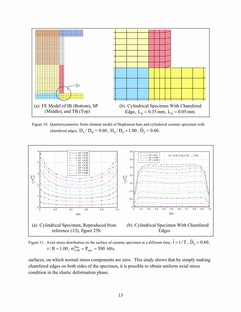
ceramic specimen with chamfered edges, S BD / D = 0.60 , S SH / D 1.00= , SD = 0.60. .........13 Figure 11. Axial stress distribution on the surface of ceramic specimen at a different time,

t t / T= , SD 0.60= , r / R 1.00= , MaxZ IB maxP 500−σ = = MPa. ....................................................13

Figure 12. Distribution of dimensionless axial stress along the length of a cylindrical specimen with and without chamfered edges. .........................................................................14

Figure 13. Distribution of axial stress in the radial direction at different Z / H locations of a cylindrical specimen with chamfered edges, t t / T 0.25.= = ..................................................15

Figure 14. The parametric definition of a cylindrical dog bone/dumbbell-shaped specimen proposed by Deltort et al..........................................................................................................16

Figure 15. Contours of axial stress distribution in the dog bone-shaped specimen at a different time............................................................................................................................17

Figure 16. Distribution of dimensionless axial stress along the length of a dog bone-shaped specimen and that for cylindrical specimens with and without chamfered edges. ..................18

Figure 17. Deviation from stress equilibrium of different specimen designs...............................18 Figure 18. A new compression SHPB experimental set-up with TT............................................20 Figure 19. Finite element model of the compression SHPB with TT...........................................22 Figure 20. Bar responses of the new compression SHPB with TT...............................................24 Figure 21. Notations for axial displacements measured at different radial locations of

different bars. ...........................................................................................................................24 Figure 22. Nonplanar interface parameter, iu , as a function of time, ceramic specimen. ...........25

v

Figure 23. Nonplanar interface parameter, iu , as a function of time, aluminum specimen.........25 Figure 24. HPB with TT: applications with direct impact and hollow cylindrical specimen......28 Figure 25. Deviation from the stress equilibrium of the ceramic specimen with a different HS

/ DS ratio, SHPB with TT.........................................................................................................29 Figure 26. Stress-strain response of SHPB with TT and comparison with classic methods, HS

/ DS, DS / DIB = 0.60.................................................................................................................30

List of Tables

Table 1. Geometric properties of the SHPB. ..................................................................................8 Table 2. Linear-elastic and elastic-plastic material constants.........................................................8 Table 3. Nonplanar bar-specimen interface parameters and fitting constants for ceramic

specimen and steel bars............................................................................................................26 Table 4. Nonplanar bar-specimen interface parameters and fitting constants for the

aluminum specimen and steel bars. .........................................................................................27

vi

Acknowledgments

This report is prepared through participation in the Composite Materials Technology Collaborative Program sponsored by the U.S. Army Research Laboratory under Cooperative Agreement DAAD19-01-2-0005. The authors gratefully acknowledge the help provided by Dr. Libo Ren in data reduction, using the dispersion correction software “Hopkinson” developed by himself and coworkers at the University of Delaware-Center for Composite Materials. Discussion and difference in opinion with Dr. Sergey L. Lopatnikov generated new ideas of Hopkinson bar experiments and analysis, and is gratefully acknowledged.

1

1. Introduction

Hopkinson bar experimental techniques (1–5) are considered the simplest high strain rate test method compared to plate impact (4) and explosive loading techniques (4, 6). Significant advances have been made in the Hopkinson Bar research field to accommodate new test methods (7–9) and new analyses techniques (10, 11). A recent critical review by the authors elucidating the 20th century advancement in Hopkinson bar techniques (12) pointed out some further areas that need improvement prior to becoming a standard test method. Two such areas are considered in the present study: the specimen deforming under uni-axial stress and the bar-specimen interfaces remaining planar throughout the duration of the test.

Finite element analysis (FEA) has been performed to study the validity of one-dimensional (1-D) assumptions (13) of compression split-Hopkinson Pressure Bar (SHPB) technique. It has been identified that the nonplanar bar-specimen assumption made in Hopkinson Bar analysis is not valid for an acoustically hard specimen with diameter smaller than the bar. As a consequence, the average strain of the specimen measured from the bar response is found unreliable. The axial stress distribution of the specimen is found to be nonuniform in the linear elastic phase of deformation; however, it is uniform in the plastic phase. It has been identified that the stress equilibrium in an elastic-plastic specimen is not achieved in the linear elastic phase of deformation; however, the deviation from equilibrium in the plastic deformation phase is constant and minimum but not absolutely zero. These important observations focused our efforts on identifying mechanisms to achieve uni-axial stress via design of the specimen geometry while simultaneously minimizing the nonplanar deformation of the bar-specimen interfaces via modifications to the test fixturing. Our objective is to achieve more accurate strain measurements enabling high strain rate properties in the elastic regime to be measured reliably.

1.1 SHPB Specimen Design

Historically, right circular cylindrical specimens have been used in the compression testing of isotropic elastic-plastic materials. However, researchers have looked at many different specimen geometries while conducting tension, shear, and torsion testing of materials under Hopkinson bar loading (4). Top hat specimen geometry for measuring tension properties using the compression SHPB is described by Lindholm and Yeakley (14). Dog bone-shaped cylindrical (15, 16) and strip specimens (17–20) have been used in tension split SHPB testing. A double-notch-shear (DNS) testing (21) and punch loading (22) are described in reference (4), where an incident bar and a transmitter tube are used in conjunction with double-notch and flat-plate specimens. A hat-shaped specimen can also be used with traditional SHPB for shear testing (4). Dog bone-shaped tubular specimens, on the other hand, are generally used for torsion testing (23) at high loading rates.

2

1.1.1 Specimen Design to Minimize Friction and Inertia

Specimen design with the objectives of minimizing friction and inertia effects has also been looked at in the past by many researchers. The maximum specimen diameter ( SD ) that can be allowed is equal to the bar diameter ( BD ). Gray (24) suggested that the radial and longitudinal inertia and friction effects can be lessened by minimizing the areal-mismatch between the bar and specimen ( S BD ~ 0.80D ); and choosing S SH /D ratio ( SH – length of the specimen) between 0.50 and 1.0, which is based on the corrections for inertia effects proposed by Davies and Hunter (25):

( ) ( ) ( )C M 2 2 2 2S S S S S Sσ (t) = σ (t) + ρ H 6 – ν D 8 × ε (t) t⎡ ⎤ ∂ ∂⎣ ⎦ , (1)

where subscript S stands for “specimen,” and superscripts C and M stand for “corrected” and “measured,” respectively. This expression predicts that the correction term will be zero, if either the strain rate is constant or the bracketed term is zero. The later condition provides the optimum ratio of the specimen for inertia effect and is expressed as follows:

S S SH /D = 3v /4 (2)

For a Poisson’s ratio of 0.333, the optimum S SH / D is 0.50. To minimize the friction effects, the S SH / D ratio should be in the range 1.50–2.00 (26). Thus the conditions for minimum friction

and inertia effects cannot be satisfied simultaneously and Gray’s (24) suggestion of 0.50 < S SH / D < 1.0 can be taken as a compromise between these two effects.

If a constant strain rate condition is used, then one can effectively use thinner specimens ( S SH / D < 0.50), and thus minimize the stress nonequilibrium in the specimen. Usually, constant strain rate conditions can be achieved through shaped incident pulses; however, the attainable strain rates in these cases are limited by the stress rate of the incident pulse (27). The optimum thickness of the specimen depends on the rise time, t, required to achieve a uni-axial stress state in the specimen. The rise time is estimated as the time required for π reverberations in the specimen (26). For a plastically deforming solid that obeys the Taylor-von Karman Theory, the rise time is given by

2 2 2S St ( H ) / ( / )≥ π ρ ∂σ ∂ε , (3)

where Sρ and SH are the density and thickness of the specimen, respectively, and /∂σ ∂ε is the stage 2 work-hardening rate of the true stress-strain diagram of the material to be tested. By decreasing the specimen thickness, it is thus possible to reduce the rise time; however, the specimen S SH / D requirement for minimizing friction and inertia effects requires that the specimen diameter also be reduced. Consequently, one needs to use a smaller diameter bar as well (to satisfy the conditions, DS ~ 0.80DB and 0.50 < S SH / D < 1.0).

3

Malinowski and Klepaczko (28) presented a combined analytical, experimental and numerical study in the determination of an optimum specimen geometry used in the SHPB test technique. In addition to specimen inertia investigated by Davies and Hunter (25), the effect of interfacial friction between the Hopkinson bars and a cylindrical specimen is considered in the analysis. A unified approach to inertia and friction is offered through the consideration of energy balance. The difference between the measured ( M

Sσ ) and correct ( CSσ ) specimen stress using “3-wave”

analysis can be expressed as follows:

( ) ( )

2M 2M C 2 2S S S SS S S S

S S S

D H 3 3 D3 H / D 12 D 16 64

⎡ ⎤⎛ ⎞µσ ρ⎢ ⎥σ − σ = + − ⋅ ε + ε + ρ ε⎜ ⎟⋅ ⎢ ⎥⎝ ⎠⎣ ⎦

, (4)

where µ is the coefficient of Coulomb friction, and both SH and SD represent their respective instantaneous values. If the optimum value S SH / D is sought by setting, M C

S S 0σ − σ = , then the following solution is obtained:

( )

( ) ( )1

3M 1 13 3S S

2 2S S SOpt

H 2 1 1 1 1D D

⎡ ⎤⎛ ⎞ ⋅µσ ⎡ ⎤⎢ ⎥= − ⋅ − + β + + + β⎜ ⎟ ⎢ ⎥ρ ⋅ ⎣ ⎦⎢ ⎥⎝ ⎠ ε + ε⎣ ⎦,

and

( )( )

2 32S S

M 2S

0.5D16 8

ε − ε⎛ ⎞ρβ = ⋅⎜ ⎟⋅µσ ⋅⎝ ⎠ ε + ε

. (5)

While the detailed analysis of equations 4 and 5 can be found in reference (28), the major conclusions about the optimum specimen S SH / D ratio are summarized here. The optimum

S SH / D is a function of coefficient of friction, specimen stress, density, strain rate, and strain acceleration. Thus, there is no universal optimum S SH / D ratio, rather it changes with ε and ε of the test for a given specimen material. Based on the fact that the optimum S SH / D ratio is a function of M

S S/σ ρ of the specimen, Malinowski and Klepaczko (28) identified three ranges of optimum S SH / D values for metals:

1. For materials with high MS S/σ ρ ratio (e.g., titanium, high-strength steel, etc.) –

S S1.0 H / D 1.5≤ ≤ .

2. For materials with medium MS S/σ ρ ratio (e.g., aluminum, copper, etc.) –

S S0.5 H / D 1.0≤ ≤ .

3. For materials with low MS S/σ ρ ratio (e.g., lead, gold, etc.) – S S0.1 H / D 0.5≤ ≤ .

In addition to the previously mentioned discussion on the optimum S SH / D ratio for metallic specimens, there are additional guidelines for soft (29) and hard (27) specimens also. Chen et al. (30) observed substantial wave attenuation in thick (0.25-in) RTV630 rubber samples

4

as compared with thin (0.06-in) samples, suggesting that depending on test temperature and specimen material, an S SH / D ratio of 0.25–0.50 can be used to minimize attenuation. Ceramic specimens, on the other hand, possess high-failure strength and relatively low-failure strain. In order to allow sufficient deformation of the specimen before failure, the recommended S SH / D ratio for ceramic specimens is usually higher than for the metallic specimens ( S S1.0 H / D 2.0< < ) (27).

1.1.2 Experimental Study on Specimen Shape and Failure

Harding (31) used waisted strip specimen (in-plane shape is rectangular and dog bone shaped through the thickness) under compression SHPB technique and found that stress equilibrium is hard to achieve. On the other hand, Harding’s compression SHPB experiments on cylindrical specimens with specimen length to diameter ratio, S SH / D = 1.0, 2.0, and 2.5 in the warp and weft directions revealed that in addition to the shear band formation, specimens with higher

S SH / D ratio introduce longitudinal splitting as an additional failure mode.

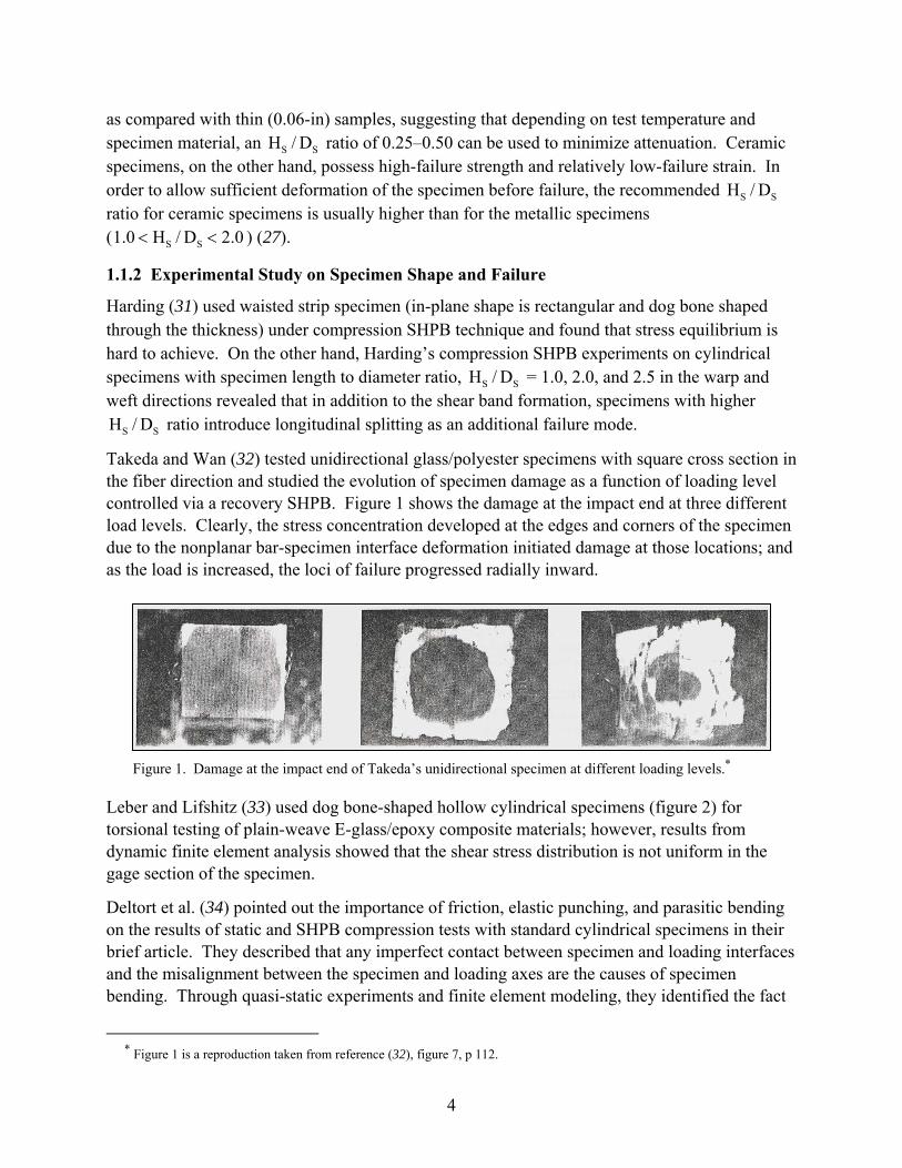
Takeda and Wan (32) tested unidirectional glass/polyester specimens with square cross section in the fiber direction and studied the evolution of specimen damage as a function of loading level controlled via a recovery SHPB. Figure 1 shows the damage at the impact end at three different load levels. Clearly, the stress concentration developed at the edges and corners of the specimen due to the nonplanar bar-specimen interface deformation initiated damage at those locations; and as the load is increased, the loci of failure progressed radially inward.

Figure 1. Damage at the impact end of Takeda’s unidirectional specimen at different loading levels.*

Leber and Lifshitz (33) used dog bone-shaped hollow cylindrical specimens (figure 2) for torsional testing of plain-weave E-glass/epoxy composite materials; however, results from dynamic finite element analysis showed that the shear stress distribution is not uniform in the gage section of the specimen.

Deltort et al. (34) pointed out the importance of friction, elastic punching, and parasitic bending on the results of static and SHPB compression tests with standard cylindrical specimens in their brief article. They described that any imperfect contact between specimen and loading interfaces and the misalignment between the specimen and loading axes are the causes of specimen bending. Through quasi-static experiments and finite element modeling, they identified the fact

* Figure 1 is a reproduction taken from reference (32), figure 7, p 112.

5

Figure 2. Dog bone-shaped hollow cylindrical

specimen geometry for torsional testing.*

that friction between specimen and interfaces and elastic punching effect lead to a heterogeneous state of specimen strain and can cause barreling of the specimen at large deformation. A new specimen design is proposed, which has a dog bone/dumbbell shape (figure 3). They performed a few quasi-static and SHPB compression experiments to prove the concept. The new specimen is found to have a problem of buckling because of its longer length.

Figure 3. New compression SHPB specimen geometry proposed by Deltort et al.† All dimensions in millimeters.

Ninan et al. (35) used both two-dimensional (2-D) plane stress and an axisymmetric model of the full SHPB and studied the effect of interface friction and incident pulse shape. The strain history of a rectangular specimen (axial dimension smaller than bar diameter) was presented at five different points, considering both frictionless and constrained boundaries. The strain history/distribution was found uniform for the frictionless case, but nonuniform for the constrained case. A conclusion was made that friction at bar-specimen interfaces may produce nonhomogeneous strain distribution in the specimen.

*Figure 2 is a reproduction taken from reference (33), figure 3, p 394. † Figure 3 is a reproduction taken from reference (34), figure 3, p C3–267.

6

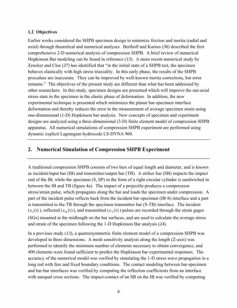
1.2 Objectives

Earlier works considered the SHPB specimen design to minimize friction and inertia (radial and axial) through theoretical and numerical analyses. Bertholf and Karnes (36) described the first comprehensive 2-D numerical analysis of compression SHPB. A brief review of numerical Hopkinson Bar modeling can be found in reference (13). A more recent numerical study by Zencker and Clos (37) has identified that “in the initial state of a SHPB test, the specimen behaves elastically with high stress triaxiality. In this early phase, the results of the SHPB procedure are inaccurate. They can be improved by well-known inertia corrections, but error remains.” The objectives of the present study are different than what has been addressed by other researchers. In this study, specimen designs are presented which will improve the uni-axial stress state in the specimen in the elastic phase of deformation. In addition, the new experimental technique is presented which minimizes the planar bar-specimen interface deformation and thereby reduces the error in the measurement of average specimen strain using one-dimensional (1-D) Hopkinson bar analysis. New concepts of specimen and experiment designs are analyzed using a three-dimensional (3-D) finite element model of compression SHPB apparatus. All numerical simulations of compression SHPB experiment are performed using dynamic explicit Lagrangian hydrocode LS-DYNA 960.

2. Numerical Simulation of Compression SHPB Experiment

A traditional compression SHPB consists of two bars of equal length and diameter, and is known as incident/input bar (IB) and transmitter/output bar (TB). A striker bar (SB) impacts the impact end of the IB, while the specimen (S, SP) in the form of a right circular cylinder is sandwiched in between the IB and TB (figure 4a). The impact of a projectile produces a compression stress/strain pulse, which propagates along the bar and loads the specimen under compression. A part of the incident pulse reflects back from the incident bar-specimen (IB-S) interface and a part is transmitted to the TB through the specimen-transmitter bar (S-TB) interface. The incident ( I (t)ε ), reflected ( R (t)ε ), and transmitted ( T (t)ε ) pulses are recorded through the strain gages (SGs) mounted at the midlength on the bar surfaces, and are used to calculate the average stress and strain of the specimen following the 1-D Hopkinson Bar analysis (24).

In a previous study (13), a quartersymmetric finite element model of a compression SHPB was developed in three dimensions. A mesh sensitivity analysis along the length (Z-axis) was performed to identify the minimum number of elements necessary to obtain convergence, and 400 elements were found sufficient to predict the Hopkinson bar experimental responses. The accuracy of the numerical model was verified by simulating the 1-D stress wave propagation in a long rod with free and fixed boundary conditions. The contact modeling between bar-specimen and bar-bar interfaces was verified by computing the reflection coefficients from an interface with unequal cross sections. The impact-contact of an SB on the IB was verified by computing

7

the stress in the bar, particle velocities of the propagating stress waves, and the duration of pulses as a function of SB lengths. The finite diameter effect in an SHPB was evaluated by the study of shaped pulses. The model was also validated for a “bars together” calibration experiment. The model was found to predict all the previously mentioned analytical problems with sufficient accuracy. This well-verified and validated model is used in the present analyses. The axis of the cylindrical specimen is taken as the Z-axis, and the axis orthogonal to the Z-axis is taken as the radial axis, r (also X and Y axes [figure 4b]). The details of the model can be found in reference (13). For completeness, a brief summary is presented next.

Figure 4. Schematic diagram of a compression SHPB and the notations used in the analyses.

A 3-D model of the SHPB is developed using 8-node solid elements. A 1-point integration scheme is used to save computational time. The longitudinal axis of the bars is taken as the geometric Z-axis. In the case of a specimen with a circular or rectangular cross section, two planes of symmetry passing through X-Z and Y-Z plane exist. In the present study, a quartersymmetric model (figure 5) with appropriate boundary conditions in the symmetric planes is used. The impact velocity of the SB is used as the initial condition, or a pressure pulse is applied on the impact face of the IB. A surface-to-surface contact interface condition without friction is defined between the bar interfaces. The specimen in the form of a right circular cylinder or a dog bone/dumbbell shape is considered.

Figure 5. Quartersymmetric model of SHPB and finite element mesh.

Striker Bar(SB)

Incident/Input Bar(IB)

Transmitter/Output Bar(TB)

Specimen(SP)

Strain Gage (SG) Strain Gage

Striker Bar(SB)

Incident/Input Bar(IB)

Transmitter/Output Bar(TB)

Specimen(SP)

Strain Gage (SG) Strain Gage

H

Z

r, X,

Y

R0

H

Z

r, X,

Y

R0

(a) Compression SHPB (b) Notations

Transmission Bar (TB)

Striker Bar (SB)

Incident Bar (IB)

Specimen (SP)

Transmission Bar (TB)

Striker Bar (SB)

Incident Bar (IB)

Specimen (SP)

8

The geometric dimensions of the model are presented in table 1; however, all of these dimensions can be varied as a test parameter. The bars remain elastic at all times during the SHPB experiment, and thus a linear-elastic isotropic material model is considered for the bars. The specimens are modeled with both linear-elastic and elastic-plastic isotropic material models. Two material parameters, Young’s modulus (E) and Poisson’s ratio (ν), are required to describe a linear-elastic model; however, two additional parameters, yield stress (σy) and tangent modulus (Et), are necessary for elastic-plastic definition. For wave propagation analysis, density (ρ) of the material is also necessary. The material properties used in the numerical simulation are listed in table 2 including the calculated bar velocity 0C E /= ρ .

Table 1. Geometric properties of the SHPB.

Parameter SB IB TB SP

Length (mm) 304.80 1524 1524 Variable

Diameter (mm) 25.40 25.40 25.40 Variable

Table 2. Linear-elastic and elastic-plastic material constants.

Material Ρ (g/cm3)

E (GPa)

ν σy (MPa)

Et (MPa)

c0 (m/s)

Inconela 8.40 201.33 0.290 — — 4895.70

Steel 7.85 206.91 0.300 830.00 0.0 5134.00

Aluminum 2.70 68.95 0.285 249.00 840.00 5053.42

Ceramic 3.95 370.00 0.220 — — 9678.37 aInconel is a registered trademark of the INCO family of companies.

In the SHPB experiment, the most common measured quantities are the impact velocity of the projectile, axial strain on the bar surface as a function of time via surface mounted SGs, and the axial and transverse strains on the specimen surface as a function of time. In the numerical experiment, displacement and velocity of nodes, strain and stress of the elements, interface forces, and material and global energies can be investigated as a function of time. Time history data of selected nodes, elements, and interfaces of interest are stored during solution and analyzed during the postprocessing phase. The validated model, as described in reference (13), is then used for detailed numerical analyses.

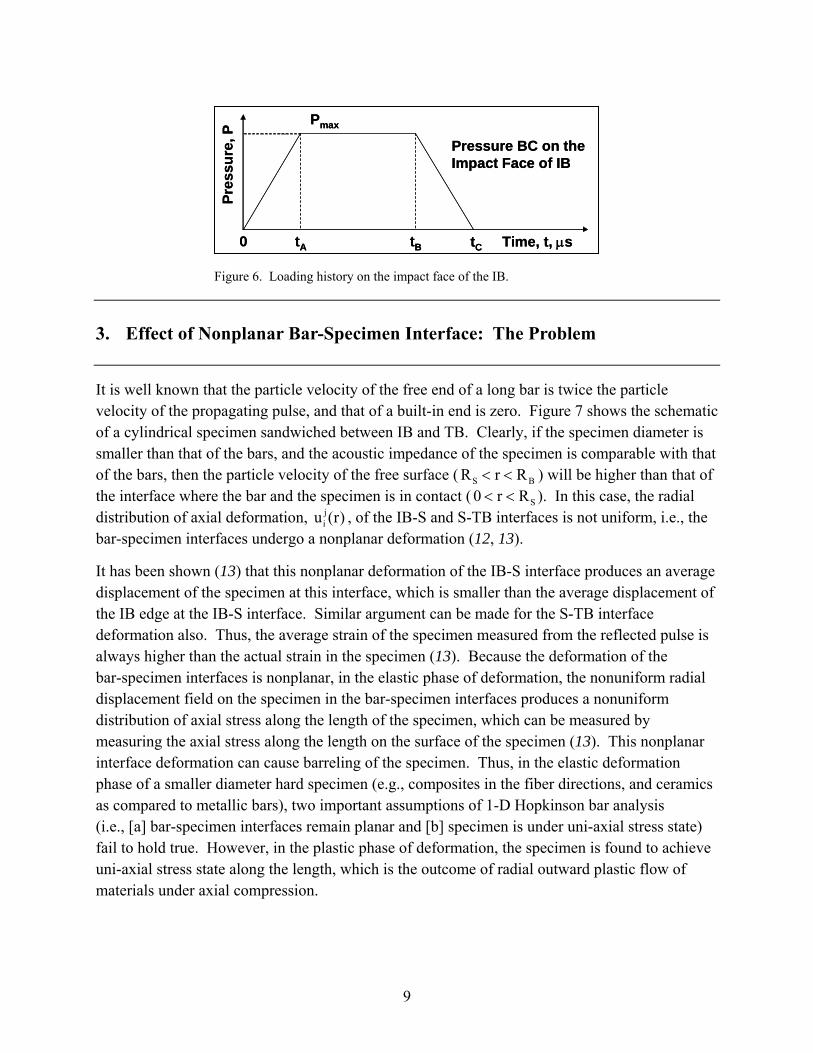
In order to enforce a known boundary condition, a parametric stress pulse is taken as the input to the impact face of the IB with four parameters: At , Bt , Ct , and maxP (figure 6). By suitable choice of these parameters: different pulse shapes can be obtained (e.g., rectangular, trapezoidal, and triangular). Detail parameters used in a numerical experiment will be described in each different case study.

9

Figure 6. Loading history on the impact face of the IB.

3. Effect of Nonplanar Bar-Specimen Interface: The Problem

It is well known that the particle velocity of the free end of a long bar is twice the particle velocity of the propagating pulse, and that of a built-in end is zero. Figure 7 shows the schematic of a cylindrical specimen sandwiched between IB and TB. Clearly, if the specimen diameter is smaller than that of the bars, and the acoustic impedance of the specimen is comparable with that of the bars, then the particle velocity of the free surface ( S BR r R< < ) will be higher than that of the interface where the bar and the specimen is in contact ( S0 r R< < ). In this case, the radial distribution of axial deformation, j

iu (r) , of the IB-S and S-TB interfaces is not uniform, i.e., the bar-specimen interfaces undergo a nonplanar deformation (12, 13).

It has been shown (13) that this nonplanar deformation of the IB-S interface produces an average displacement of the specimen at this interface, which is smaller than the average displacement of the IB edge at the IB-S interface. Similar argument can be made for the S-TB interface deformation also. Thus, the average strain of the specimen measured from the reflected pulse is always higher than the actual strain in the specimen (13). Because the deformation of the bar-specimen interfaces is nonplanar, in the elastic phase of deformation, the nonuniform radial displacement field on the specimen in the bar-specimen interfaces produces a nonuniform distribution of axial stress along the length of the specimen, which can be measured by measuring the axial stress along the length on the surface of the specimen (13). This nonplanar interface deformation can cause barreling of the specimen. Thus, in the elastic deformation phase of a smaller diameter hard specimen (e.g., composites in the fiber directions, and ceramics as compared to metallic bars), two important assumptions of 1-D Hopkinson bar analysis (i.e., [a] bar-specimen interfaces remain planar and [b] specimen is under uni-axial stress state) fail to hold true. However, in the plastic phase of deformation, the specimen is found to achieve uni-axial stress state along the length, which is the outcome of radial outward plastic flow of materials under axial compression.

0 tB tC Time, t, µstA

Pres

sure

, P Pressure BC on the Impact Face of IB

Pmax

0 tB tC Time, t, µstA

Pres

sure

, P Pressure BC on the Impact Face of IB

Pmax

10

Figure 7. Nonplanar bar-specimen interface deformation model of a small diameter hard specimen: j

iu – axial displacements in Z-direction; subscripts i = C, D, and E represent bar-center, specimen-edge, and bar-edge, respectively; superscripts j = 1 and 2; “1” = IB-S interface; “2” = S-TB interface.*

The nonplanar deformation of bar-specimen interface is related with the nonuniform axial stress distribution in the specimen. To correct this problem, one can design a new experiment such that the bar-specimen interface remains plane at all time during dynamic deformation of the specimen, or can design a specimen such that the axial stress distribution in the specimen is uniform. In the following sections, new specimen and experiment design is presented, which improves the uni-axial stress distribution in the specimen and provides better planar bar-specimen interface conditions.

4. Uni-Axial Stress Along the Specimen Through Specimen Design: Partial Solution

The nonplanar deformation of the bar-specimen interfaces is identified as the main reason for nonuniform axial stress distribution along the length of the specimens. A numerical simulation with a cylindrical ceramic specimen of specimen diameter to bar diameter ratio, DS /DB = 0.60, and specimen length to specimen diameter ratio, HS /DS = 1.00, which is equivalent to the dimensionless specimen length, ( ) ( ) ( )2

S S B S S S B SD D D H D D D H 0.60,= = ⋅ = has been

*Adapted from references (12) and (13).

r, X, Y

Z

DB

DS

HS

uE1

uD1

uC1

RB

RS

uE2

uD2

uC2

0

1

2

IB TB

SP

r, X, Y

Z

DB

DS

HS

uE1

uD1

uC1

RB

RS

uE2

uD2

uC2

0

1

2

IB TB

SP

11

performed with a triangular input stress pulse ( At 99= µs, Bt 101= µs, Ct = 200 µs, and Pmax = 500 MPa); parameters are described in figure 6 of duration T = 200 µs. Detailed results of this simulation are presented in reference (13). The IB and TB ( BD 25.4= mm) considered in this simulation were made from steel (see table 2 for properties). The cross section of the bar is modeled with 195 elements, and the specimen cross-section has one-to-one node connectivity for stable contact modeling. The incident, reflected and transmitted stress in the bars, is presented in figure 8a as dotted lines with open symbols. It is clear from figure 8a that the specimen is loaded under compression during the first half of the incident pulse ( 0 t / T 0.50< < ), and the second half of the pulse represents unloading ( 0.50 t / T 1.00< < ). Figure 9a shows the contours of stress distribution in the specimen at three different times ( t / T 0.15, 0.30, 0.45= ) during the ramp-loading phase. The stress amplitude is highest at time, t / T 0.45= , and the stress concentration is visible at the edges of the specimen. A similar profile is also obtained by Anderson et al. (38) while modeling the compression of cylindrical specimen with truncated cones as loading block in the SHPB setting. Figure 9 also shows that the stress on the free surfaces ( S BR r R< < ) of the bar-specimen interfaces is zero.

Figure 8. Numerical Hopkinson bar responses for two different test cases.

4.1 Specimen Design 1: Cylindrical Specimen With Chamfered Edges

The nonplanar deformation model presented in figure 7 suggests that a specimen with curved loading faces can eliminate the nonuniform axial stress distribution in the specimen. While the shape of the curve to which the specimen loading surfaces should be machined can be determined by solving the nonlinear contact problem, it is obvious that this solution process is extensive in nature. To demonstrate the concept, a cylindrical specimen with chamfered edges is considered instead (figure 8b). The finite element model of this chamfered specimen is presented in figure 10. The geometry of the chamfer can be described by two variables, LR and LH, as shown in figure 8b.

(a) Bar Responses

-600

-450

-300

-150

0

150

0 100 200 300 400 500 600 700

ReflectedPulses

IncidentPulses

TransmittedPulses

Solid Lines with Solid Symbols:Cylindrical Specimenwith Chamfered Edges

Dotted Lines with Open Symbols:Cylindrical Specimen

Time, t, µs.

Stre

ss in

the

Bar,

σ Z, M

Pa.

LR

LH

Z

r, X, YLR

LH

Z

r, X, Y

RL - Dimension along radius,

HL - Dimension along length (b) Notations – Chamfered Specimen;

12

t/T = 0.15 t/T = 0.30 t/T = 0.45t/T = 0.15 t/T = 0.30 t/T = 0.45 t/T = 0.15 t/T = 0.30 t/T = 0.45t/T = 0.15 t/T = 0.30 t/T = 0.45 (a) Cylindrical Specimen (b) Specimen With Chamfered Edge

Fringe Levels: Axial Compressive Stress, Zσ , MPa

1: 0 ~ 100 2: 100 ~ 300 3: 300 ~ 500 4: 500 ~ 700

5: 700 ~ 900 6: 900 ~ 1100 7: 1100 ~ 1300 8: 1300 ~ 1500

9: 1500 ~ 1700 10: 1700 ~ 1900 11: 1900 ~ 2100 12: 2100 ~ 2300

Figure 9. Contours of axial stress distribution in the specimen at a different time.

The numerical model of the chamfered specimen is loaded with the same boundary condition as in the case of a pure cylindrical specimen. The reflected and transmitted stresses in the bars (figure 8a, solid lines with solid symbols) appear to be a little different than the case of a cylindrical specimen. The contour of axial stresses at different times in the case of the specimen with chamfered edges (figure 9b) appears to be more uniform than the cylindrical specimen. It has been shown in reference (13) that the uniformity of the distribution of the axial stress in the specimen along the length can be represented by plotting the axial stresses on the surface of the specimen along the length as a function of time (figure 11a). In the elastic phase of deformation, the axial stress distribution on the surface of cylindrical specimen is found to be nonuniform at all time. The axial stress near the bar-specimen contact interfaces is higher than the midlength of the specimen, and the distribution has an elliptical shape. The distribution of axial stresses on the surface of a cylindrical specimen with chamfered edges is shown in figure 11b. As expected, the stress distribution on the surface of the specimen is almost uniform along the length of the specimen, except at the chamfered edges. At the chamfered edges, there are additional free

13

(a) FE Model of IB (Bottom), SP

(Middle), and TB (Top) (b) Cylindrical Specimen With Chamfered

Edge, RL 0.35= mm, HL 0.05= mm.

Figure 10. Quartersymmetric finite element model of Hopkinson bars and cylindrical ceramic specimen with chamfered edges, S BD / D = 0.60 , S SH / D 1.00= , SD = 0.60.

(a) Cylindrical Specimen, Reproduced from (b) Cylindrical Specimen With Chamfered reference (13), figure 25b. Edges

Figure 11. Axial stress distribution on the surface of ceramic specimen at a different time, t t / T= , SD 0.60= , r / R 1.00= , Max

Z-IB maxP 500σ = = MPa.

surfaces, on which normal stress components are zero. This study shows that by simply making chamfered edges on both sides of the specimen, it is possible to obtain uniform axial stress condition in the elastic deformation phase.

0

1

2

3

4

5

0 0.2 0.4 0.6 0.8 1.0

t/T = 0.05t/T = 0.10t/T = 0.15t/T = 0.20t/T = 0.25t/T = 0.30t/T = 0.35t/T = 0.40t/T = 0.45

Z/H.

σ Z/σZ-

IBM

ax

0

0.5

1.0

1.5

2.0

2.5

3.0

3.5

0 0.1 0.2 0.3 0.4 0.5 0.6 0.7 0.8 0.9 1.0

t/T = 0.0t/T = 0.05t/T = 0.50

t/T = 0.05, 0.10, 0.15, ...., 0.50

Z/H.

σ Z/σZ-

IBM

ax.

14

In reference (13), it has been shown that the nonuniform distribution of axial stress on the surface of cylindrical specimen has self-similar behavior under ramp loading in the elastic phase of deformation, which can be shown by normalizing the axial stress by that at the midlength of the specimen (figure 12). In figure 12, the self-similar behavior of axial stress on the surface of a cylindrical specimen with chamfered edges is also presented. This figure shows the benefit of a chamfered specimen in attaining the uniform stress distribution in most part of a cylindrical specimen.

Figure 12. Distribution of dimensionless axial stress along the length of a cylindrical specimen with and without chamfered edges.

The axial stress distribution along the radial direction of the specimen at different Z / H locations of a cylindrical specimen at time t = t / T = 0.25 is presented in figure 13. In figure 13a, the axial stress is normalized with the maximum axial stress in the incident pulse.

The axial stress distribution in the radial direction is almost uniform in the range, 0.10 < Z / H < 0.90, which is also evident from figure 12. In figure 13b, the axial stress is normalized with the axial stress at location r / R = 0.025 and plotted as a map along the length of the specimen. This figure clearly shows that the axial stress distribution is uniform over the specimen length except for a small region around the chamfered edged. It has been shown in reference (13) that the uniform distribution of axial stress on the surface of a cylindrical specimen along the length guarantees the overall uniformity of axial stress in the specimen (in the plastic deformation phase). Figure 13 proves the validity of that general statement in the

0

0.2

0.4

0.6

0.8

1.0

1.2

1.4

1.6

1.8

2.0

0 0.1 0.2 0.3 0.4 0.5 0.6 0.7 0.8 0.9 1.0

t/T = 0.05, 0.10, 0.15, ...., 0.50

CylindricalSpecimenwithChamferedEdges

CylindricalSpecimen

Z/H.

σ Z/σZZ/

H =

0.5

0 .

15

Figure 13. Distribution of axial stress in the radial direction at different Z / H locations of a cylindrical specimen with chamfered edges, t t / T 0.25.= =

elastic deformation phase in case of a cylindrical specimen with chamfered edges. Chamfering the edges of the specimen can thus effectively minimize the problem of nonuniform axial stress distribution of a small diameter cylindrical specimen. The analysis of the dog bone/dumbbell-shaped specimen design suggested by Deltort et al. (34) is presented next.

4.2 Specimen Design 2: Dog Bone/Dumbbell-Shaped Cylindrical Specimen

One can analyze the distribution of axial stress on the surface of a cylindrical specimen in the elastic deformation phase (figure 12) and can heuristically make a hypothesis that a traditional dog bone/dumbbell shape cylindrical specimen can also provide uniform axial stress distribution on the surface of the specimen in the gage section. It is also obvious that a specimen with a diameter equal to the bar minimizes the nonplanar deformation of the bar-specimen interfaces (12, 13). The cylindrical dog bone/dumbbell-shaped specimen proposed by Deltort et al. (34) also considered the end of the specimen to be of equal diameter to the bars. This specimen and associated parameters to define the specimen geometry are presented in figure 14. Two important parameters of the dog bone specimen are the length of the right circular cylinder part at the specimen ends, LF, (which will be in contact with the bars), and the length of the parabolic section, LC, of the specimen. The length of the cylindrical gage section is denoted by usual nomenclature, HS.

To be consistent with our analyses of cylindrical specimens with and without chamfered edges, the specimen dimensionless parameters are kept unchanged (i.e., DS / DB = 0.60, HS / DS = 1.00,

SD 0.60= ). Because the specimen aspect ratio is taken as HS / DS = 1.00, the total length of the dog bone-shaped specimen is longer than the cylindrical specimens.

0

0.5

1.0

1.5

2.0

2.5

3.0

3.5

4.0

0 0.1 0.2 0.3 0.4 0.5 0.6 0.7 0.8 0.9 1.0

Z/H = 0.01Z/H = 0.06Z/H = 0.11Z/H = 0.24Z/H = 0.49Z/H = 0.74Z/H = 0.99

r/R.

σ Z/σZ-

IBM

ax.

0.0

0.1

0.2

0.3

0.4

0.5

0.6

0.7

0.8

0.9

1.0

0 0.1 0.2 0.3 0.4 0.5 0.6 0.7 0.8 0.9 1.0

2

1

0

2

1

r/R.

Z/H

.

t/T = 0.25

025.0/ =RrZ

Z

σσ

025.0/ =RrZ

Z

σσ

0.0

0.1

0.2

0.3

0.4

0.5

0.6

0.7

0.8

0.9

1.0

0 0.1 0.2 0.3 0.4 0.5 0.6 0.7 0.8 0.9 1.0

2

1

0

2

1

r/R.

Z/H

.

t/T = 0.25

025.0/ =RrZ

Z

σσ

025.0/ =RrZ

Z

σσ

(a) Axial Stress Normalized with MaxZ-IBσ (b) Axial Stress Normalized with r / R 0.025

Z=σ

16

Figure 14. The parametric definition of a cylindrical dog bone/dumbbell-shaped specimen proposed by Deltort et al. (34).

A finite element model of the dog bone-shaped specimen is developed by keeping the same strategy of one-to-one correspondence of nodes between the contact interfaces and is presented in figure 15a. Both the bar and specimen cross-section is modeled using 144 elements. The specimen parameters have been marked on the FE model, and the different sections and interfaces are highlighted. Similar loads and boundary conditions are used as in the case of specimen design 1. Figure 15b shows the contour of axial stress distribution in the dog bone-shaped specimen at three different times, as is also presented in previous cases (figure 9). The range of fringes is also the same for comparison with figure 9. The axial stress distribution of the dog bone-shaped specimen is superior to that of the cylindrical specimen with chamfered edges. The distribution of axial stress on the surface of the dog bone-shaped specimen along the length is presented in figure 16, where the Z-coordinate at the beginning of the gage section is taken as zero to make a comparison with the cylindrical specimens. The results for cylindrical specimens with and without chamfer are also plotted for comparison. There still remains some nonhomogenous distribution of axial stress at the beginning of the gage section; however, the overall distribution is superior to that of the cylindrical specimen with the chamfered edge.

A dog bone-shaped shaped cylindrical specimen can provide a uni-axial stress condition in the specimen in the elastic deformation phase; however, the calculation of the specimen average strain from bar responses becomes problematic due to the presence of the additional length of the specimen in addition to the gage section. However, because the specimen has uni-axial stress state over the gage length, SGs can be mounted on the surface of the specimen to measure the specimen strain, which is also true for the case of the cylindrical specimen with chamfered edges. It is interesting to note that, in testing of ceramic materials, SGs are used on the specimen to measure the specimen strain along with shaped pulses (27). However, uncertainty remains in selecting an SG of specific gage length for a specific specimen length, even if one decides to bond the SG in the midlength of the specimen. From the present analysis, a major conclusion

LC LFHS

DS DB

r, X, Y

Z

LC LFHS

DS DB

r, X, Y

Z

17

IB

TB

LF

LC

HS

IB

TB

LF

LC

HS

7.62mm

8.28mm

7.77mm

9.34mm

12.7mm

LC = 7.62mm

LF = 6.35mm

7.62mm

8.28mm

7.77mm

9.34mm

12.7mm

LC = 7.62mm

LF = 6.35mm

t/T = 0.15 t/T = 0.45t/T = 0.30t/T = 0.15 t/T = 0.45t/T = 0.30

(a) FE Model of the Dog Bone Specimen

(b) Axial Stress Distribution

Fringe Levels: Axial Compressive Stress, Zσ , MPa

1: 0 ~ 100 2: 100 ~ 300 3: 300 ~ 500 4: 500 ~ 700

5: 700 ~ 900 6: 900 ~ 1100 7: 1100 ~ 1300 8: 1300 ~ 1500

9: 1500 ~ 1700 10: 1700 ~ 1900 11: 1900 ~ 2100 12: 2100 ~ 2300

Figure 15. Contours of axial stress distribution in the dog bone-shaped specimen at a different time.

can be made that Hopkinson Bar testing of linear-elastic materials (e.g., composites in fiber direction and ceramics) can be performed while satisfying the uni-axial stress condition in the elastic phase of deformation if a chamfered or dog bone-shaped specimen is used. The other conclusion is that one can use SG to measure specimen strain with confidence, knowing the fact that the specimen is under uni-axial stress state in case of a chamfered and a dog bone/dumbbell-shaped specimen.

Both of the specimen designs have their own limitations. The chamfered cylindrical specimen does not guarantee the planar bar interface condition, and thus the solution is not complete. The dog bone-shaped specimen having equal diameter guarantees planar bar-specimen condition, however, requires an additional SG to measure the strain in the specimen. It is also important that the specimen remains under stress equilibrium. The deviation of stress equilibrium in the specimen is usually characterized by the factor ( ) ( )avg 1 2 1 2R / 2 F F / F F= ∆σ σ = ⋅ − + (12, 13) and is presented in figure 17 for all three cases. The forces, 1F and 2F , at the IB-S and S-TB interfaces, are taken from the time history of contact forces at the corresponding interfaces.

18

0

0 . 2

0 . 4

0 . 6

0 . 8

1 . 0

1 . 2

1 . 4

1 . 6

1 . 8

2 . 0

0 0 . 1 0 . 2 0.3 0.4 0.5 0.6 0.7 0.8 0 . 9 1 . 0

Dog Bone-ShapedCylindricalSpecimen

t/T = 0.10, 0.15, ...., 0.45

C y l i n d r i calS p e c i m enw i t h C h a m f e redE d g e s

C y l i n dricalS p e c imen

Z/H.

σ Z / σ Z Z / H =

0 . 5 0 .

Figure 16. Distribution of dimensionless axial stress along the length of a dog bone-shaped specimen and that for cylindrical specimens with and without chamfered edges.

0

0 . 1

0 . 2

0 . 3

0 . 4

0 . 5

0 . 6

0 . 7

0 . 8

0 . 9

1 . 0

0 0 . 0 5 0 . 1 0 0.15 0.20 0.25 0.30 0.35 0.40 0 . 4 5 0 . 5 0

Dog Bone Cyl. Speci m e n Chamfered Cyl. Spec i m e n Cylindrical Specimen

t/T.

R = ∆ σ / σ a v g = 2 ( F 1 - F 2 ) / ( F 1 + F 2 ) .

Figure 17. Deviation from stress equilibrium of different specimen designs.

19

It has been shown by the authors (13) that the specimen is not under stress equilibrium at anytime as can also be seen from figure 17. It is interesting that the cylindrical specimen with chamfered edges does not provide any better stress equilibrium for the specimen. However, the dog bone/dumbbell shaped specimen, being longer in length, has the deviation from equilibrium, which is much higher than the cylindrical specimens with chamfered edges. In both the cases, additional considerations should be undertaken to improve the stress equilibrium in the specimen. In separate works (39, 40), analytical techniques have been proposed to address the issues related to deviation of stress equilibrium. However, in general, better stress equilibrium can be achieved by using thinner specimens (12).

5. Planar Bar-Specimen Interface Condition Through Experiment Design: Complete Solution

The nonplanar deformation model of a small diameter hard specimen is presented in figure 7 and is also discussed in references (12, 13, 34). The main reason for the nonplanar deformation of the bar-specimen interface is that the free end of the IB, which is not in contact with the specimen (RS < r < RB), moves with higher particle velocity than the portion in contact with the specimen (0 < r < RS), as described in figure 7. If one uses a specimen with diameter equal to the bar (DS = DB), the bar-specimen interfaces will remain planar. However, if high strain rate stress-strain diagram up to the failure of the specimen is sought, a realistic engineering practice is to use a small diameter specimen such that the stress level in the specimen is sufficiently high to cause damage or failure. If a smaller diameter specimen is used, ideally one can use a hollow cylindrical tube to load the free end of the specimen. In that case, the transmitter bar diameter should be equal to the specimen diameter to support the specimen on the transmission end. A new compression SHPB experimental technique is proposed in this report for the first time to guarantee the planar bar-specimen interface condition, and is presented in figure 18.

5.1 Compression SHPB With a TT

The new compression SHPB has several unique features, which include a transmitter /transmission bar (TB) that is equal to the SP diameter, or a little greater diameter than the specimen to accommodate the radial expansion due to Poisson’s effect. It has a TT with an inner diameter a little greater than the TB, such that the TB can have a sliding fit inside the TT; and the outer diameter of the TT is equal to the diameter of the IB. The length of the TT should be more than 4× the SB length, and should be approximately half the length of the TB. Independent SGs should be mounted on the IB, TT, and TB. Figure 18 shows that both the specimen and the TT are in contact with the IB. When the incident pulse reaches the IB-S/IB-TT interface, a part of it is transmitted to the TT and a part to the specimen. If the TT and the IB are made from the same material, the reflection coefficient of the area of IB that is in contact with the TT is zero (acoustic impedance of the IB and TT tube being the same, i.e., IB IB 0IB TT 0TT TTZ c c Z= ρ = ρ = ).

20

(a) Schematic Diagram

(b) Notations

Figure 18. A new compression SHPB experimental set-up with TT.

The reflection coefficient of the part of IB that is in contact with the specimen depends on the impedance of the specimen. If the impedance of the specimen is 50% of the bar, then the reflection coefficient of the IB-S contact area is 1

3− (negative one-third), and if it is 50% more than the bar, then the reflection coefficient is 1

5+ (positive one-fifth). Because the reflection from the IB-TT interface is zero, the reflected pulse recorded by the SG mounted on the IB surface will consist only of the reflections from the IB-S contact interface and from the free surface of the IB if there is any clearance between the specimen and the TT. Thus, the particle velocities at IB-S and IB-TT interfaces can be expressed as

IB-S IB IBI R1 0IB (t) (t)u = –c × ε – ε⎡ ⎤⎣ ⎦ (6)

and

IB-TT IB TTI T1 0IB 0TT(t) (t)u = –c ×ε = –c ×ε , (7)

and the corresponding displacements as

t

IB-S IB IBI R1 0IB (t) (t)u c dt⎡ ⎤⎣ ⎦= − ⋅ ε − ε ⋅∫ (8)

and

SB IB TT TBSP

SG SG

SGSB IB TT TBSP

SG SG

SG

IB TT

TB

SP

TTIBu −1

SIBu −1

TBIBu −2

1 2

( )tIBIε

( )tIBRε

( )tTTTε

( )tTBTε

IB TT

TB

SP

TTIBu −1

SIBu −1

TBIBu −2

1 2

( )tIBIε

( )tIBRε

( )tTTTε

( )tTBTε

21

t t

IB-TT IB TTI T1 0IB 0TT(t) (t)u c dt c dt= − ⋅ ε ⋅ = − ⋅ ε ⋅∫ ∫ , (9)

where subscript 1 represents the IB-S/IB-TT interface, and the superscripts denote the location where the properties are measured at. If the IB-S/IB-TT interface remains planar then the following equity should exist:

IB-S IB-TT1 1u = u . (10)

If this equity exists, then either of equations 8 or 9 can be taken as the displacement of the IB-S/IB-TT interface, otherwise one can take an algebraic average as the displacement at this interface:

( )IB-S/ IB-TT IB-TT IB-S1 1 1u u u 2= + . (11)

A complex stress wave reverberation in the specimen takes place, and the stress wave is transmitted to the TB. The particle velocity and displacement at the S-TB interface can then be expressed as

S-TB TBT2 0TB (t)u c= − ⋅ε (12)

and

t

S-TB TBT2 0TB (t)u c dt= − ⋅ ε ⋅∫ , (13)

where subscript 2 represents the S-TB interface.

It is well known that the stress wave propagation in finite diameter bars is dispersive (3, 41), and thus a dispersion correction of the strain signals recorded on IB, TT, and TB should be performed (10, 12). It is important to mention that the dispersion correction methodology automatically performs the time sifting of incident, reflected and transmitted pulses to a common zero, and makes the algebraic manipulation easy. Once the dispersion correction procedure is performed, the average strain of the specimen can be expressed as

( )S-TB IB-S/ IB-TTS 2 1 S(t) u u Hε = − . (14)

Because the free end of the IB-S interface is loaded with the TT and the TB diameter is equal to the specimen diameter, it is anticipated that the bar-specimen interfaces will remain planar at all time. Thus the major problem of nonplanar bar-specimen interface condition of a smaller diameter hard specimen can be resolved by the new compression SHPB with TT.

Following the 1-D stress wave propagation assumptions (12), the forces in the IB-S/IB-TT interface and S-TB interface can be expressed as

IB IB TT1 IB IB I R TT TT TF (t) A E (t) (t) A E (t)⎡ ⎤= ε + ε − ε⎣ ⎦ , (15)

22

and

TB2 TB TB TF (t) A E (t)= ε . (16)

The average stress in the specimen then can be expressed as

[ ]S 1 2 S(t) F (t) F (t) 2 Aσ = + ⋅ , (17)

which is equivalent to the “3-wave” analysis as described by Gray (24). Because equation (17) use four different measured strains to calculate the average specimen stress, this analysis can be termed as “4-wave” analysis.

The use of a TT is reported in literature by Harding and Huddart (21) in the dynamic punch shear testing technique, and by Nemat-Nasser et al. (8) in the tri-axial Hopkinson bar test technique. However, the unique use of TT to guarantee the planar bar-specimen interface condition is reported in this report for the first time. The numerical experiment of this new SHPB design is presented next to provide the proof of concept and validity of analysis.

5.2 Numerical Simulation of Compression SHPB With TT

The cross section of the specimen and the TB is modeled with 280 and 300 elements, respectively; while the IB and TT cross sections are modeled with 540 and 240 elements, respectively. Along the length of the IB and TB, 400 elements are used as described for the earlier case; however, 200 elements along the length of TT are used. A specimen with chamfered edges is used in this model, which guarantees the uni-axial stress along the length of the specimen. The parameters of the chamfered specimen are the same as described earlier. Figure 19 shows the FE model at the bar-specimen interfaces location. Properties of steel are used to model the bars, and the specimen is modeled with elastic-plastic aluminum and elastic ceramic materials.

IB SP

TT

TT

TBIB SP

TT

TT

TB

Figure 19. Finite element model of the compression SHPB with TT.

23

The geometric dimensions of the SHPB with TT model are as follows: IBL = 1524 mm, IBD = 25.4 mm, TTL = 562 mm, ID

TTD = 15.875 mm, ODTTD = 25.4 mm, TBL = 1524 mm,

TBD = 15.1 mm, SH = 15.24 mm, and SD = 15.1 mm. These dimensions for the bars and the specimen represent a realistic experiment, where the specimen diameter is a little less than the TB, and the diameter of the TB is also a little less than the inner diameter of the TT. A triangular input stress pulse ( At 99= µs, Bt 101= µs, Ct 200= µs, and maxP 500= MPa) of duration T 200= µs is used at the impact end of the projectile. The bar responses (element stresses on the bar surface at midlength) are presented in figure 20 with aluminum and ceramic specimens for the IB, TB, and TT. Note that the reflected and transmitted pulses measured at midlength of the IB and TB have the same time references; however, the transmitted pulse measured at midlength of the TT appears early in time because the length of TT is half of the IB. In the case of the aluminum specimen, a reflected pulse with a nearly constant amplitude up to 500 µs represents the elastic deformation phase, and the increase in amplitude after that represents the plastic deformation, which is also evident from the transmitted pulse. However, for the ceramic specimen, the reflected pulse has near zero amplitude because the impedance ratio of steel and ceramic is 1.054. As described earlier, the stress pulse in the TT has the same order of magnitude as the incident pulse and can be used to measure the displacement of the IB-S/IB-TT interface of the specimen.

The stresses in the bars are dispersion corrected (12), and then the time-shifted stresses are converted to strains in the bars. Equations 6–17 are used in calculating the average strain and stress in the specimen. Before presenting the stress-strain data, one needs to prove that the bar-specimen interface is planar and the specimen is under uni-axial stress. In addition, one also needs to comment on the stress equilibrium. If these three basic assumptions made in 1-D Hopkinson bar analysis hold true, then the experiment is considered as a valid experiment.

Three dimensionless nonplanar interface parameters, iu – i = IB, TT, TB, can be defined to express the deviation from the planar interface condition for the bar-specimen interfaces.

( )C A AIB Z Z Z(t)u u u u= − , (18)

( )C B BTT Z Z Z(t)u u u u= − , (19)

and

( )E D DTB Z Z Z(t)u u u u= − , (20)

where, the displacement components, jZu , are outlined in figure 21, and j = A, B, C, D, E.

24

Figure 20. Bar responses of the new compression SHPB with TT.

Figure 21. Notations for axial displacements measured at different radial locations of different bars.

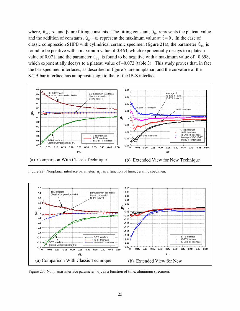
Figures 22 and 23 show the time history of the dimensionless nonplanar interface parameters for ceramic and aluminum specimens, respectively. In these figures, the nonplanar interface parameters IBu , TTu , and TBu (given by equations 18–20) for the new compression SHPB with TT are presented and denoted by IB-S/IB-TT interface, IB-TT interface, and S-TB interface, respectively. In addition, the nonplanar interface parameters at IB-S interface and S-TB interface for classic SHPB with cylindrical specimens are also presented. The nonplanar interface parameters have maximum value at small displacements, which correspond to small time ( t 0≈ ) and exponentially decrease to plateau level at large displacements, and can be expressed as

( ) ti i0

ˆˆ ˆu t u e−β⋅= + α ⋅ , (21)

-600

-400

-200

0

200

400

600

0 100 200 300 400 500 600 700

TransmissionTube Response

TransmittedPulse

ReflectedPulse

IncidentPulse

Time, t, µs.

Stre

ss in

the

Bar

s, σ

, ΜΠ

α.

-600

-400

-200

0

200

400

600

0 100 200 300 400 500 600 700

TransmissionTube Response

TransmittedPulse

ReflectedPulse

IncidentPulse

Time, t, µs.

Stre

ss in

the

Bars

, σ, M

Pa.

(a) With Aluminum Specimen (b) With Ceramic Specimen

IB

TT

TB

SP

AZu

CZu

BZu

DZu

EZu

IB

TT

TB

SP

AZu

CZu

BZu

DZu

EZu

25

(a) Comparison With Classic Technique

where, i0u , α , and β are fitting constants. The fitting constant, i0u represents the plateau value and the addition of constants, i0u + α represent the maximum value at t 0= . In the case of classic compression SHPB with cylindrical ceramic specimen (figure 21a), the parameter IBu is found to be positive with a maximum value of 0.463, which exponentially decays to a plateau value of 0.071, and the parameter TBu is found to be negative with a maximum value of −0.698, which exponentially decays to a plateau value of −0.072 (table 3). This study proves that, in fact the bar-specimen interfaces, as described in figure 7, are nonplanar, and the curvature of the S-TB bar interface has an opposite sign to that of the IB-S interface.

Figure 22. Nonplanar interface parameter, iu , as a function of time, ceramic specimen.

Figure 23. Nonplanar interface parameter, iu , as a function of time, aluminum specimen.

iu

-0.7

-0.6

-0.5

-0.4

-0.3

-0.2

-0.1

0

0.1

0.2

0.3

0.4

0.5

0 0.05 0.10 0.15 0.20 0.25 0.30 0.35 0.40 0.45 0.50

S-TB InterfaceIB-TT InterfaceIB-S/IB-TT Interface

Bar-Specimen InterfacesNew CompressionSHPB with TT

S-TB InterfaceClassic Compression SHPB

IB-S InterfaceClassic Compression SHPB

t/T.

iu

-0.7

-0.6

-0.5

-0.4

-0.3

-0.2

-0.1

0

0.1

0.2

0.3

0.4

0.5

0 0.05 0.10 0.15 0.20 0.25 0.30 0.35 0.40 0.45 0.50

S-TB InterfaceIB-TT InterfaceIB-S/IB-TT Interface

Bar-Specimen InterfacesNew CompressionSHPB with TT

S-TB InterfaceClassic Compression SHPB

IB-S InterfaceClassic Compression SHPB

t/T.

iu

-0.04

-0.03

-0.02

-0.01

0

0.01

0.02

0.03

0.04

0 0.05 0.10 0.15 0.20 0.25 0.30 0.35 0.40 0.45 0.50

S-TB InterfaceIB-TT InterfaceIB-S/IB-TT InterfaceAverage of IB-S/IB-TT and IB-TT Interfaces

Average ofIB-S/IB-TT andIB-TT Interfaces

IB-TT Interface

S-TB Interface

IB-S/IB-TT Interface

t/T.

iu

-0.04

-0.03

-0.02

-0.01

0

0.01

0.02

0.03

0.04

0 0.05 0.10 0.15 0.20 0.25 0.30 0.35 0.40 0.45 0.50

S-TB InterfaceIB-TT InterfaceIB-S/IB-TT InterfaceAverage of IB-S/IB-TT and IB-TT Interfaces

Average ofIB-S/IB-TT andIB-TT Interfaces

IB-TT Interface

S-TB Interface

IB-S/IB-TT Interface

t/T.

(a) Comparison With Classic Technique (b) Extended View for New Technique

iu

-0.7

-0.6

-0.5

-0.4

-0.3

-0.2

-0.1

0

0.1

0.2

0.3

0.4

0.5

0 0.05 0.10 0.15 0.20 0.25 0.30 0.35 0.40 0.45 0.50

S-TB InterfaceIB-TT InterfaceIB-S/IB-TT Interface

Bar-Specimen InterfacesNew CompressionSHPB with TT

S-TB InterfaceClassic Compression SHPB

IB-S InterfaceClassic Compression SHPB

t/T.

iu

-0.7

-0.6

-0.5

-0.4

-0.3

-0.2

-0.1

0

0.1

0.2

0.3

0.4

0.5

0 0.05 0.10 0.15 0.20 0.25 0.30 0.35 0.40 0.45 0.50

S-TB InterfaceIB-TT InterfaceIB-S/IB-TT Interface

Bar-Specimen InterfacesNew CompressionSHPB with TT

S-TB InterfaceClassic Compression SHPB

IB-S InterfaceClassic Compression SHPB

t/T.

iu

-0.20

-0.18

-0.16

-0.14

-0.12

-0.10

-0.08

-0.06

-0.04

-0.02

0

0.02

0.04

0.06

0.08

0.10

0 0.05 0.10 0.15 0.20 0.25 0.30 0.35 0.40 0.45 0.50

S-TB InterfaceIB-TT InterfaceIB-S/IB-TT Interface

t/T.

iu

-0.20

-0.18

-0.16

-0.14

-0.12

-0.10

-0.08

-0.06

-0.04

-0.02

0

0.02

0.04

0.06

0.08

0.10

0 0.05 0.10 0.15 0.20 0.25 0.30 0.35 0.40 0.45 0.50

S-TB InterfaceIB-TT InterfaceIB-S/IB-TT Interface

t/T.

(b) Extended View for New (a) Comparison With Classic Technique

26

Table 3. Nonplanar bar-specimen interface parameters and fitting constants for ceramic specimen and steel bars.

Ceramic Specimens

Parameters

Classic SHPB New SHPB With TT

IBu TBu IBu TBu

i0u 0.0709 −0.0716 0.0031 −0.0034 α 0.3920 −0.6260 0.0209 −0.0354 β 7.34 7.57 26.4 8.22

In the case of the new compression SHPB with TT and with ceramic specimen, the calculated values of the nonplanar interface parameters are an order of magnitude lower than the classic case; however, these are not absolutely zero. A little free surface on the IB-S/IB-TT interface and the specimen with different acoustic impedance than the bars are the main reasons for the finite but relatively smaller values of the nonplanar interface parameters. Figure 21b shows a close-up view of these parameters. Table 3 shows the fitting parameters of the nonplanar interface parameters for IB-S and S-TB interfaces. The plateau value at IB-S/IB-TT is found to be (ûIB0 = 0.0031), which is only 4.4% as compared to the classic case (ûIB0 = 0.0709). The maximum value in this case is found to be (ûIB0 + a = 0.024), which is ~5.2% of the classic value (ûIB0 + a = 0.463). Similar reduction is observed in the S-TB interface. This study validates the hypothesis made prior to the numerical experiment that the new compression SHPB with TT will guarantee a planar-bar-specimen interface condition for small-diameter-hard specimens in the elastic phase of deformation. In a realistic experimental setup, the specimen diameter should be a little less than the transmission bar, and there would be a little free surface on the IB-S/IB-TT interface, and thus the bar-specimen interfaces, will not be perfectly nonplanar. In the case of ceramic specimens and steel bars, the classic method provides 46%–70% error in small strain measurement and ~7% error for large strain measurements. However, this new technique with TT will provide much better accuracy than the classic method with the limit of 2%–4% error for very small strain measurement and 0.31%–0.34% error for relatively larger strains.

It is interesting to note that the error in the IB-TT interface is similar (same order of magnitude) to that of the IB-S/IB-TT interface, but is negative instead of positive. If equation 11 is used to calculate the average displacement at the IB-S/IB-TT interface, the error will be minimum (near zero) as shown in figure 22b by the legend “Average of the IB-S/IB-TT and IB-TT Interfaces.” It has been shown that the error in the S-TB interface is an order of magnitude smaller in the case of the SHPB with TT; the use of equation 14 will provide a sufficiently accurate measurement of strain in the elastic deformation phase (small strain) of a ceramic (linear-elastic) specimen.

The aluminum specimen is acoustically softer than the bars, and thus the curvature of the IB-S/IB-TT interface, in the case of SHPB with TT, is found opposite to that of the classic case (figure 23b, table 4). This implies that the particle velocity at the center of the IB

27

Table 4. Nonplanar bar-specimen interface parameters and fitting constants for the aluminum specimen and steel bars.

Aluminum Specimens

Parameters

Classic SHPB New SHPB With TT

IBu TBu IBu TBu

i0u −0.0114 −0.0164 −0.0147 0.0050

α 0.2280 −0.7250 −0.1570 −0.0404 β 5.27 6.52 15.6 4.55

(in contact with the specimen) is higher than the edge of the IB. In other wards, the curvature of the IB-S interface has the same shape and sign as that of the S-TB interface. In this case, the displacement measured at the IB-S/IB-TT interface will be smaller than the average displacement of the specimen, and consecutively the strain measured using equation 8 will be smaller than the specimen strain. This error in displacement measurement (under prediction) at the IB-S/IB-TT interface has the same order of magnitude as compared to the classic case (over prediction); however, the amplitude error is a little smaller. On the other hand, the error in the S-TB interface is greatly improved by the new SHPB with TT method.

The amplitude of the stress pulse in the TT has the same order of magnitude as that of the incident pulse. A close examination of figure 22b and 23b reveals that the error in the IB-TT interface is negative and an order of magnitude smaller as compared to the classic case. Thus, the stress pulse of TT alone can be used to measure the displacement (equation 9) of the IB-S/IB-TT interface, irrespective of the type of the specimen. In this case, the IB responses (incident and reflected pulses) are redundant, which suggests that the length of the IB can be arbitrary. If the length of the IB is considered zero, then the compression SHPB with TT reduces to a direct impact Hopkinson pressure bar (HPB) with TT (figure 24a). One of the problems of direct impact HPB is that the displacement of the impact face of the specimen cannot be measured without a high-speed camera. If a direct impact HPB with TT is used, the displacement of the impact end of the specimen can be measured from the TT response (equation 9), and as usual, the displacement of the S-TB interface can be estimated from the TB response (equation 13).

The analysis and numerical results presented can be applied to a hollow cylindrical specimen with some changes. Figure 24b shows the application of a hollow cylindrical specimen in conjunction with an SHPB with TT and with a direct impact HPB with TT. Materials with low Poisson’s ratio, e.g., metal foams, can be used as hollow cylindrical specimens. Additional cylindrical enclosures may be used to characterize materials under confinement. The new compression SHPB with TT (figure 18) and the new direct impact HPB with TT (figure 24a) guarantee the planar bar-specimen interface condition within reasonable engineering accuracy (<5%). In addition, the direct impact HPB with TT eliminates the age-old problem of

28

(a) Direct Impact HPB with TT

(b) Hollow Cylindrical Specimen with the new SHPB or Direct Impact HPB with TT

Figure 24. HPB with TT: applications with direct impact and hollow cylindrical specimen.

displacement measurement at the impact end of the specimen. Because the cylindrical specimen with chamfered edges provides uni-axial stress distribution along the length of the specimen under elastic deformation phase, the use of a cylindrical specimen with chamfered edges in conjunction with the new SHPB with TT satisfies the planar bar-specimen interface condition at all time. However, the problem of stress equilibrium in the specimen remains (figure 17). The accurate construction of a stress-strain diagram in the linear-elastic deformation phase should accurately predict the average stress in the specimen in addition to the accurate prediction of small strain/elastic deformation. The stress equilibrium in the specimen is usually not achieved (24, 27, 37) in the initial phase of elastic deformation (figure 17). It is a usual practice to use specimens with HS / DS ~ 1.00 in most SHPB applications; however, thinner specimens can provide better stress equilibrium. If thinner specimens are used, 0.01 < HS / DS < 0.10, the uni-axial stress condition of the specimen changes to plane-strain condition, and in this case, friction and radial inertia effects become important. The new SHPB with TT is designed for small strain measurement in the linear-elastic deformation phase, and it can be assumed that the

SB TT TBSP

SG

SGSB TT TBSP

SG

SG

IB or SB TT TBHollow Cylindrical

SpecimenIB or SB TT TBHollow Cylindrical

Specimen

29

friction and radial inertia effects are negligible. With this assumption, the effect of specimen thickness on the nonequilibrium stress parameter, R, is determined for three different ceramic specimens with chamfered edges, HS / DS = 1.00, 0.50, 0.25, and is presented in figure 25.

0

0.05

0.10

0.15

0.20

0.25

0.30

0.35

0.40

0.45

0.50

0 0.05 0.10 0.15 0.20 0.25 0.30 0.35 0.40 0.45 0.50

HS/DS = 0.25HS/DS = 0.50HS/DS = 1.00

Chamfered SpecimenSHPB with TT

t/T.

R =

∆σ/

σ avg =

2(F

1 - F 2)/(

F 1 + F

2).

Figure 25. Deviation from the stress equilibrium of the ceramic

specimen with a different HS / DS ratio, SHPB with TT.

Figure 25 shows that the decrease in the specimen HS / DS ratio decreases the nonequilibrium stress parameter, R; however, nonequilibrium exists (37). Thus, one can plot the time-averaged nonequilibrium stress and strain data to represent engineering stress-strain relationships of the material at high strain rate (figure 26). The numerical bar responses are corrected for dispersion following the methodology proposed by Lifshitz and Leber (10). In addition, the dispersion correction algorithm for cylindrical tubes and rods proposed by Ren et al. (41) using the M-H shell model (42, 43) is also used.

The linear-elastic modulii of ceramic and aluminum used in the simulations were 370 GPa and 69 GPa, respectively. In the case of ceramic specimen (figure 26a), the modulii obtained from the simulation in the cases of classic 1-wave, 3-wave, and SHPB with TT analyses are 158, 208, and 502 GPa, respectively, which corresponds to the ratio of theoretical modulus vs. simulated modulus, ETheo / ESimu 0.427, 0.562, and 1.357, respectively. The ratios ETheo / ESimu for the aluminum specimen (figure 26b) in the previously mentioned cases are 0.790, 0.764, and 1.635, respectively. Clearly, the classic 1- and 3-wave analyses predict higher strains due to the nonplanar interface condition and thus lower linear-elastic modulus. The new SHPB with TT overpredicts the modulus, which proves the validity of the assumption that the bar-specimen interfaces are nonplanar. The impedance mismatch between the SP and IB, and IB and TT (note that we used steel TT) is identified as the source of this error. If the impedance of the TT is matched with that of the specimen, this error might reduce significantly, and these issues will be addressed elsewhere.

30

Figure 26. Stress-strain response of SHPB with TT and comparison with classic methods, HS / DS, DS / DIB = 0.60.

Zhao and Gary (44) and Zhao (45) proposed a combined analytical-numerical-experimental approach for the small strain measurement using the SHPB technique, which is computationally extensive and requires parametric evaluation of several parameters of a rate-sensitive material model, however, is considered the state-of-the-art solution of the problem. The new SHPB with TT and with the chamfered cylindrical specimen provides an experimental way of measuring small linear-elastic deformation, while satisfying all the major assumptions made in the 1-D SHPB analysis.

6. Summary

Extensive numerical analyses are carried out in the design of Hopkinson bar specimens and in new experiments that satisfy the uni-axial stress condition in the specimen and the planar bar-specimen conditions. It has been shown that a right cylindrical specimen with a chamfered specimen with a diameter smaller than the bars improves the uni-axial stress condition in the specimen. The new SHPB with TT and direct impact HPB with TT experimental techniques provide the planar bar-specimen interface condition much better than the traditional method. These new experimental techniques provide a way for small-strain measurement with sufficient engineering accuracy. The new direct impact HPB with TT solves the age-old problem of the displacement measurement at the impact end of the specimen. One-dimensional Hopkinson bar analysis is modified for the analysis of the new SHPB with TT technique. The new data analysis together with dispersion correction methodology is applied to reduce the numerical bar responses in to stress-strain diagrams. Results show that the new SHPB with TT provides better planar bar-specimen interface conditions, however, overpredicts the linear-elastic modulus, which can further be modified though the selection of impedance-matched TT.

0

200

400

600

800

1000

1200

1400

1600

1800

2000

0 0.001 0.002 0.003 0.004 0.005 0.006 0.007 0.008 0.009 0.010

SHPB with TT: Dispersed, E = 502 GPa.3-wave: Dispersed, E = 208 GPa.1-wave: Dispersed, E = 158 GPa.

Engineering Strain, ε, mm/mm.

Eng

inee

ring

Stre

ss, σ

, MPa

.

0

50

100

150

200

250

300

350

400

0 0.005 0.010 0.015 0.020 0.025 0.030 0.035 0.040 0.045 0.050

SHPB with TT: Dispersed, E = 112.8 GPa.3-wave: Dispersed, E = 52.7 GPa.1-wave: Dispersed, E = 54.5 GPa.

Engineering Strain, ε, mm/mm.

Eng

inee

ring

Stre

ss, σ

, MPa

.

(a) Ceramic Specimen (b) Aluminum Specimen

31

7. References

1. Hopkinson, B. A Method of Measuring the Pressure Produced in the Detonation of High Explosives or by the Impact of Bullets. Philosophical Transactions of the Royal Society of London, Series A, Containing Papers of a Mathematical or Physical Character 1914, 213, 437–456.

2. Kolsky, H. An Investigation of the Mechanical Properties of Materials at Very High Rates of Loading. Proc. Phys. Soc., London, II-B 1949, 62, 676–700.

3. Davies, R. M. A Critical Study of the Hopkinson Pressure Bar. Philosophical Transactions of the Royal Society of London, Series A, Mathematical and Physical Sciences 1948, 240 (821), 375–457.

4. Mechanical Testing and Evaluation, ASM Handbook, Volume 8; AMS International: Materials Park, OH, 2000.

5. Meyers, M. A. Dynamic Behavior of Materials; John Wiley & Sons: New York, 1994.

6. Daniel, I. M.; LaBedz, R. H.; Liber, T. New Methods for Testing Composites at Very High Strain Rates. Experimental Mechanics 1981, 21 (2), 71–77.

7. Nemat-Nasser, S.; Issacs, J. B.; Starrett, J. E. Hopkinson Techniques for Dynamic Recovery Experiments. Proceedings of the Royal Society of London, Series A 1991, 453, 371–391.

8. Nemat-Nasser, S.; Isaacs, J.; Rome J. Triaxial Hopkinson Techniques, Mechanical Testing and Evaluation, ASM Handbook, Volume 8; ASM International: Materials Park, OH, 2000; pp 516–518.

9. Chen, W.; Zhang, B.; Forrestal, M. J. A Split Hopkinson Bar Technique for Low Impedance Materials. Experimental Mechanics 1999, 39, 1–5.

10. Lifshitz, J. M.; Leber, H. Data Processing in the Split Hopkinson Pressure Bar Tests International Journal of Impact Engineering 1994, 15 (6), 723–733.

11. Bussac, M. N.; Collet, P.; Gary, G.; Othman, R. An Optimization Method for Separating and Rebuilding One-Dimensional Dispersive Waves From Multi-Point Measurements: Application to Elastic or Viscoelastic Bars. Journal of the Mechanics and Physics of Solids 2002, 50, 321–349.

12. Gama, B. A.; Lopatnikov, S. L.; Gillespie, J. W., Jr. Hopkinson Bar Experimental Technique: A Critical Review. Applied Mechanics Review August 2003.

32

13. Gama, B. A.; Lopatnikov, S. L.; Gillespie, J. W., Jr. Numerical Hopkinson Bar Analysis: Validity of One-Dimensional Assumptions. ASC 2003 Conference, Gainesville, FL, 20–22 October 2003.

14. Lindholm, U. S.; Yeakley, L. M. High Strain Rate Testing: Tension and Compression. Experimental Mechanics 1968, 8, 1–9.

15. Nicholas, T. Tensile Testing of Materials at High Rates of Strain. Experimental Mechanics 1980, 21, 177–185.

16. Noble, J. P.; Goldthorpe, B. D.; Church, P.; Harding, J. The Use of the Hopkinson Bar to Validate Constitutive Relations at High Rates of Strain. Journal of Mechanics and Physics of Solids 1999, 47, 1187–1206.

17. Rodriguez, J.; Chocron, I. S.; Martinez, M. A.; Sanchez Galvez, V. High Strain Rate Properties of Aramid and Polyethylene Woven Fabric Composites. Composites, Part B, 1996, 27B, 147–154.

18. Chocron Benloulo, I. S.; Rodriguez, J.; Martinez, M. A.; Sanchez Galvez, V. Dynamic Tensile Testing of Aramid and Polyethylene Fiber Composites. International Journal of Impact Engineering 1997, 19 (2), 135–146.

19. Melin, L. G.; Asp, L. E. Effects of Strain Rate on Transverse Tension Properties of a Carbon/Epoxy Composite: Studied by Moire Photography. Composites, Part A, 1999, 30, 305–316.

20. Eskandari, H.; Nemes, J. A. Dynamic Testing of Composite Laminates With a Tensile Split Hopkinson Bar. Journal of Composite Materials 2000, 33 (4), 260–273.

21. Harding, J.; Huddart, J. The Use of the Double-Notch Shear Test in Determining the Mechanical Properties of Uranium at Very High Rates of Strain. Proceedings of the 2nd International Conference on Mechanical Properties at High Rates of Strain; Harding, J., Ed., The Institute of Physics: London, 1980, vol. 47, pp 49–61.

22. Ferguson, W. G.; Hauser, J. E.; Dorn, J. E. The Dynamic Punching of Metals, Dislocation Damping in Zink Single Crystals. Britt. J. Appl. Phys. 1967, 18, 411–417.

23. Gilat, A. Torsional Kolsky Bar Testing, Mechanical Testing and Evaluation, ASM Handbook, Volume 8, ASM International: Materials Park, OH, 2000; pp 505–515.

24. Gray, G. T., III. Classic Split-Hopkinson Pressure Bar Testing, Mechanical Testing and Evaluation, ASM Handbook, Volume 8; ASM International: Materials Park, OH, 2000; pp 462–476.

25. Davies, E. D. H.; Hunter, S. C. The Dynamic Compression Testing of Solids by the Method of Split Hopkinson Pressure Bar (SHPB). J. Mech. Phys. Solids 1963, 11, 155–179.

33

26. Follansbee, P. S. The Hopkinson Bar, Mechanical Testing and Evaluation, ASM Handbook, Volume 8; ASM International: Materials Park, OH, 1995; pp 198–203.

27. Subhash, G.; Ravichandran, G. Split-Hopkinson Pressure Bar Testing of Ceramics, Mechanical Testing and Evaluation, ASM Handbook, Volume 8; ASM International: Materials Park, OH, 2000; pp 488–496.

28. Malinowski, J. Z.; Klepaczko, J. R. Unified Analytic and Numerical Approach to Specimen Behavior in the Split Hopkinson Pressure Bar. International Journal of Mechanical Sciences 1986, 28 (6), 381–391.

29. Gray, G. T., III. Split-Hopkinson Pressure Bar Testing of Soft Materials, Mechanical Testing and Evaluation, ASM Handbook, Volume 8; ASM International: Materials Park, OH, 2000; pp 488–496.

30. Chen, W.; Zhang, B.; Forrestal, M. J. A Split Hopkinson Bar Technique for Low Impedance Materials. Experimental Mechanics 1999, 39, 1–5.

31. Harding, J. Effect of Strain Rate and Specimen Geometry on the Compressive Strength of Woven Glass-Reinforced Epoxy Laminates. Composites 1993, 24 (4), 323–332.

32. Takeda, N.; Wan, L. Impact Compression Damage Evolution in Unidirectional Glass Fiber Reinforced Polymer Composites, ASME, AD in High Strain Rate Effects on Polymer, Metal and Ceramic Matrix Composites and Other Advanced Materials 1995, 48, 109–113.

33. Leber, H.; Lifshitz, J. M. Interlaminar Shear Behavior of Plain-Weave GRP at Static and High Rates of Strain. Composites Science and Technology 1996, 56 (4), 391–405.

34. Deltort, B.; Neme, A.; Tanguy, B. New Specimen Geometry for Compression Hopkinson Bars. Journal De Physique, IV 1997, 7 (3), C3-265–C3-270.

35. Ninan, L.; Tsai, J.; Sun, C. T. Use of Split Hopkinson Pressure Bar for Testing Off-Axis Composites. International Journal of Impact Engineering 2001, 25, 291–313.

36. Bertholf, L. D.; Karnes, C. H. Two-Dimensional Analysis of the Split Hopkinson Pressure Bar System. Journal of Mechanics and Physics of Solids 1975, 23, 1–19.

37. Zencker, U.; Clos, R. Limiting Conditions for Compression Testing of Flat Specimens in the Split Hopkinson Pressure Bar. Experimental Mechanics 1999, 39 (4), 343–348.

38. Anderson C. E., Jr.; O’Donoghue, P. E.; Lankford, J.; Walker, J. D. Numerical Simulation of SHPB Experiments for the Dynamic Compressive Strength and Failure of Ceramics. International Journal of Fracture 1992, 55, 193–208.

34

39. Lopatnikov, S. L.; Gama, B. A.; Krauthauser, C.; Gillespie, J. W., Jr. On the Classic Split-Hopkinson Pressure Bar (SHPB) Analysis. Technical Physics Letters 2004, 30 (2), 39–46.

40. Pochhammer, L. Uber Fortplanzungsgeschwindigkeiten kleiner Schwindungen in einem unbegrenzten isotropen Kreiszylinder. Journal reine angewandte Mathematik (Creele) 1876, 81, 324.

41. Ren, L.; Larson, M.; Gama, B. A.; Gillespie, J. W., Jr. Wave Dispersion in Cylindrical Tubes: Applications to Hopkinson Pressure Bar Experimental Techniques. International Journal of Impact Engineering, submitted for publication, May 2003.

42. Herrmann, G.; Mirsky, I. Three-Dimensional and Shell-Theory Analysis of Axially Symmetric Motions of Cylinders. Journal of Applied Mechanics 1956, 23, 563–568.

43. Mirsky, I.; Herrmann, G. Axially Symmetric Motions of Thick Cylindrical Shells. Journal of Applied Mechanics 1958, 25, 97–102.

44. Zhao, H.; Gary, G. On the Use of SHPB Techniques to Determine the Dynamic Behavior of Materials in the Range of Small Strains. International Journal of Solids and Structures 1996, 33 (23), 3363–3375.

45. Zhao, H. A Study on Testing Techniques for Concrete-Like Materials Under Compressive Impact Loading. Cement and Concrete Composites 1998, 20, 293–299.

NO. OF NO. OF COPIES ORGANIZATION COPIES ORGANIZATION

35

1 DEFENSE TECHNICAL (PDF INFORMATION CTR ONLY) DTIC OCA 8725 JOHN J KINGMAN RD STE 0944 FT BELVOIR VA 22060-6218 1 COMMANDING GENERAL US ARMY MATERIEL CMD AMCRDA TF 5001 EISENHOWER AVE ALEXANDRIA VA 22333-0001 1 INST FOR ADVNCD TCHNLGY THE UNIV OF TEXAS AT AUSTIN 3925 W BRAKER LN STE 400 AUSTIN TX 78759-5316 1 US MILITARY ACADEMY MATH SCI CTR EXCELLENCE MADN MATH THAYER HALL WEST POINT NY 10996-1786 1 DIRECTOR US ARMY RESEARCH LAB IMNE AD IM DR 2800 POWDER MILL RD ADELPHI MD 20783-1197 3 DIRECTOR US ARMY RESEARCH LAB AMSRD ARL CI OK TL 2800 POWDER MILL RD ADELPHI MD 20783-1197 3 DIRECTOR US ARMY RESEARCH LAB AMSRD ARL CS IS T 2800 POWDER MILL RD ADELPHI MD 20783-1197

ABERDEEN PROVING GROUND 1 DIR USARL AMSRD ARL CI OK TP (BLDG 4600)

NO. OF NO. OF COPIES ORGANIZATION COPIES ORGANIZATION

36

1 DIRECTOR US ARMY RESEARCH LAB AMSRD ARL SE L D SNIDER 2800 POWDER MILL RD ADELPHI MD 20783-1197 1 DIRECTOR US ARMY RESEARCH LAB AMSRD ARL SE DE R ATKINSON 2800 POWDER MILL RD ADELPHI MD 20783-1197 5 DIRECTOR US ARMY RESEARCH LAB AMSRD ARL WM MB A ABRAHAMIAN M BERMAN M CHOWDHURY T LI E SZYMANSKI 2800 POWDER MILL RD ADELPHI MD 20783-1197 1 COMMANDER US ARMY MATERIEL CMD AMXMI INT 5001 EISENHOWER AVE ALEXANDRIA VA 22333-0001 2 PM MAS SFAE AMO MAS MC PICATINNY ARSENAL NJ 07806-5000 3 COMMANDER US ARMY ARDEC AMSTA AR CC M PADGETT J HEDDERICH H OPAT PICATINNY ARSENAL NJ 07806-5000 2 COMMANDER US ARMY ARDEC AMSTA AR AE WW E BAKER J PEARSON PICATINNY ARSENAL NJ 07806-5000

1 COMMANDER US ARMY ARDEC AMSTA AR FSE PICATINNY ARSENAL NJ 07806-5000 1 COMMANDER US ARMY ARDEC AMSTA AR TD PICATINNY ARSENAL NJ 07806-5000 13 COMMANDER US ARMY ARDEC AMSTA AR CCH A F ALTAMURA M NICOLICH M PALATHINGUL D VO R HOWELL A VELLA M YOUNG L MANOLE S MUSALLI R CARR M LUCIANO E LOGSDEN T LOUZEIRO PICATINNY ARSENAL NJ 07806-5000 1 COMMANDER US ARMY ARDEC AMSTA AR CCH P J LUTZ PICATINNY ARSENAL NJ 07806-5000 1 COMMANDER US ARMY ARDEC AMSTA AR FSF T C LIVECCHIA PICATINNY ARSENAL NJ 07806-5000 1 COMMANDER US ARMY ARDEC AMSTA ASF PICATINNY ARSENAL NJ 07806-5000

NO. OF NO. OF COPIES ORGANIZATION COPIES ORGANIZATION

37

1 COMMANDER US ARMY ARDEC AMSTA AR QAC T C J PAGE PICATINNY ARSENAL NJ 07806-5000 1 COMMANDER US ARMY ARDEC AMSTA AR M D DEMELLA PICATINNY ARSENAL NJ 07806-5000 3 COMMANDER US ARMY ARDEC AMSTA AR FSA A WARNASH B MACHAK M CHIEFA PICATINNY ARSENAL NJ 07806-5000 2 COMMANDER US ARMY ARDEC AMSTA AR FSP G M SCHIKSNIS D CARLUCCI PICATINNY ARSENAL NJ 07806-5000 2 COMMANDER US ARMY ARDEC AMSTA AR CCH C H CHANIN S CHICO PICATINNY ARSENAL NJ 07806-5000 1 COMMANDER US ARMY ARDEC AMSTA AR QAC T D RIGOGLIOSO PICATINNY ARSENAL NJ 07806-5000 1 COMMANDER US ARMY ARDEC AMSTA AR WET T SACHAR BLDG 172 PICATINNY ARSENAL NJ 07806-5000

1 US ARMY ARDEC INTELLIGENCE SPECIALIST AMSTA AR WEL F M GUERRIERE PICATINNY ARSENAL NJ 07806-5000 10 COMMANDER US ARMY ARDEC AMSTA AR CCH B P DONADIA F DONLON P VALENTI C KNUTSON G EUSTICE K HENRY J MCNABOC G WAGNECZ R SAYER F CHANG PICATINNY ARSENAL NJ 07806-5000 6 COMMANDER US ARMY ARDEC AMSTA AR CCL F PUZYCKI R MCHUGH D CONWAY E JAROSZEWSKI R SCHLENNER M CLUNE PICATINNY ARSENAL NJ 07806-5000 1 PM ARMS SFAE GCSS ARMS BLDG 171 PICATINNY ARSENAL NJ 07806-5000 1 COMMANDER US ARMY ARDEC AMSTA AR WEA J BRESCIA PICATINNY ARSENAL NJ 07806-5000 1 PM MAS SFAE AMO MAS PICATINNY ARSENAL NJ 07806-5000

NO. OF NO. OF COPIES ORGANIZATION COPIES ORGANIZATION

38

1 PM MAS SFAE AMO MAS CHIEF ENGINEER PICATINNY ARSENAL NJ 07806-5000 1 PM MAS SFAE AMO MAS PS PICATINNY ARSENAL NJ 07806-5000 2 PM MAS SFAE AMO MAS LC PICATINNY ARSENAL NJ 07806-5000 1 COMMANDER US ARMY ARDEC PRODUCTION BASE MODERN ACTY AMSMC PBM K PICATINNY ARSENAL NJ 07806-5000 1 COMMANDER US ARMY TACOM PM COMBAT SYSTEMS SFAE GCS CS 6501 ELEVEN MILE RD WARREN MI 48397-5000 1 COMMANDER US ARMY TACOM AMSTA SF WARREN MI 48397-5000 1 DIRECTOR AIR FORCE RESEARCH LAB MLLMD D MIRACLE 2230 TENTH ST WRIGHT PATTERSON AFB OH 45433-7817 1 OFC OF NAVAL RESEARCH J CHRISTODOULOU ONR CODE 332 800 N QUINCY ST ARLINGTON VA 22217-5600 1 US ARMY CERL R LAMPO 2902 NEWMARK DR CHAMPAIGN IL 61822

1 COMMANDER US ARMY TACOM PM SURVIVABLE SYSTEMS SFAE GCSS W GSI H M RYZYI 6501 ELEVEN MILE RD WARREN MI 48397-5000 1 COMMANDER US ARMY TACOM CHIEF ABRAMS TESTING SFAE GCSS W AB QT T KRASKIEWICZ 6501 ELEVEN MILE RD WARREN MI 48397-5000 1 COMMANDER WATERVLIET ARSENAL SMCWV QAE Q B VANINA BLDG 44 WATERVLIET NY 12189-4050 1 TNG, DOC, & CBT DEV ATZK TDD IRSA A POMEY FT KNOX KY 40121 2 HQ IOC TANK AMMUNITION TEAM AMSIO SMT R CRAWFORD W HARRIS ROCK ISLAND IL 61299-6000 2 COMMANDER US ARMY AMCOM AVIATION APPLIED TECH DIR J SCHUCK FT EUSTIS VA 23604-5577 1 NSWC DAHLGREN DIV CODE G06 DAHLGREN VA 22448 2 US ARMY CORPS OF ENGR CERD C T LIU CEW ET T TAN 20 MASSACHUSETTS AVE NW WASHINGTON DC 20314

NO. OF NO. OF COPIES ORGANIZATION COPIES ORGANIZATION

39

1 US ARMY COLD REGIONS RSCH & ENGRNG LAB P DUTTA 72 LYME RD HANOVER NH 03755 14 COMMANDER US ARMY TACOM AMSTA TR R R MCCLELLAND D THOMAS J BENNETT D HANSEN AMSTA JSK S GOODMAN J FLORENCE K IYER D TEMPLETON A SCHUMACHER AMSTA TR D D OSTBERG L HINOJOSA B RAJU AMSTA CS SF H HUTCHINSON F SCHWARZ WARREN MI 48397-5000 14 BENET LABS AMSTA AR CCB R FISCELLA M SOJA E KATHE M SCAVULO G SPENCER P WHEELER S KRUPSKI J VASILAKIS G FRIAR R HASENBEIN AMSTA CCB R S SOPOK E HYLAND D CRAYON R DILLON WATERVLIET NY 12189-4050 1 USA SBCCOM PM SOLDIER SPT AMSSB PM RSS A J CONNORS KANSAS ST NATICK MA 01760-5057

1 NSWC TECH LIBRARY CODE 323 17320 DAHLGREN RD DAHLGREN VA 22448 2 USA SBCCOM MATERIAL SCIENCE TEAM AMSSB RSS J HERBERT M SENNETT KANSAS ST NATICK MA 01760-5057 2 OFC OF NAVAL RESEARCH D SIEGEL CODE 351 J KELLY 800 N QUINCY ST ARLINGTON VA 22217-5660 1 NSWC CRANE DIVISION M JOHNSON CODE 20H4 LOUISVILLE KY 40214-5245 2 NSWC U SORATHIA C WILLIAMS CD 6551 9500 MACARTHUR BLVD WEST BETHESDA MD 20817 2 COMMANDER NSWC CARDEROCK DIVISION R PETERSON CODE 2020 M CRITCHFIELD CODE 1730 BETHESDA MD 20084 8 DIRECTOR US ARMY NGIC D LEITER MS 404 M HOLTUS MS 301 M WOLFE MS 307 S MINGLEDORF MS 504 J GASTON MS 301 W GSTATTENBAUER MS 304 R WARNER MS 305 J CRIDER MS 306 2055 BOULDERS RD CHARLOTTESVILLE VA 22911-8318

NO. OF NO. OF COPIES ORGANIZATION COPIES ORGANIZATION

40

1 NAVAL SEA SYSTEMS CMD D LIESE 1333 ISAAC HULL AVE SE 1100 WASHINGTON DC 20376-1100 1 EXPEDITIONARY WARFARE DIV N85 F SHOUP 2000 NAVY PENTAGON WASHINGTON DC 20350-2000 8 US ARMY SBCCOM SOLDIER SYSTEMS CENTER BALLISTICS TEAM J WARD W ZUKAS P CUNNIFF J SONG MARINE CORPS TEAM J MACKIEWICZ BUS AREA ADVOCACY TEAM W HASKELL AMSSB RCP SS W NYKVIST S BEAUDOIN KANSAS ST NATICK MA 01760-5019 7 US ARMY RESEARCH OFC A CROWSON H EVERETT J PRATER G ANDERSON D STEPP D KISEROW J CHANG PO BOX 12211 RESEARCH TRIANGLE PARK NC 27709-2211 1 AFRL MLBC 2941 P ST RM 136 WRIGHT PATTERSON AFB OH 45433-7750 1 DIRECTOR LOS ALAMOS NATL LAB F L ADDESSIO T 3 MS 5000 PO BOX 1633 LOS ALAMOS NM 87545

8 NSWC J FRANCIS CODE G30 D WILSON CODE G32 R D COOPER CODE G32 J FRAYSSE CODE G33 E ROWE CODE G33 T DURAN CODE G33 L DE SIMONE CODE G33 R HUBBARD CODE G33 DAHLGREN VA 22448 1 NSWC CARDEROCK DIVISION R CRANE CODE 6553 9500 MACARTHUR BLVD WEST BETHESDA MD 20817-5700 1 AFRL MLSS R THOMSON 2179 12TH ST RM 122 WRIGHT PATTERSON AFB OH 45433-7718 2 AFRL F ABRAMS J BROWN BLDG 653 2977 P ST STE 6 WRIGHT PATTERSON AFB OH 45433-7739 5 DIRECTOR LLNL R CHRISTENSEN S DETERESA F MAGNESS M FINGER MS 313 M MURPHY L 282 PO BOX 808 LIVERMORE CA 94550 1 AFRL MLS OL L COULTER 5851 F AVE BLDG 849 RM AD1A HILL AFB UT 84056-5713 1 OSD JOINT CCD TEST FORCE OSD JCCD R WILLIAMS 3909 HALLS FERRY RD VICKSBURG MS 29180-6199

NO. OF NO. OF COPIES ORGANIZATION COPIES ORGANIZATION

41

3 DARPA M VANFOSSEN S WAX L CHRISTODOULOU 3701 N FAIRFAX DR ARLINGTON VA 22203-1714 2 SERDP PROGRAM OFC PM P2 C PELLERIN B SMITH 901 N STUART ST STE 303 ARLINGTON VA 22203 1 OAK RIDGE NATL LAB R M DAVIS PO BOX 2008 OAK RIDGE TN 37831-6195 1 OAK RIDGE NATL LAB C EBERLE MS 8048 PO BOX 2008 OAK RIDGE TN 37831 3 DIRECTOR SANDIA NATL LABS APPLIED MECHS DEPT MS 9042 J HANDROCK Y R KAN J LAUFFER PO BOX 969 LIVERMORE CA 94551-0969 1 OAK RIDGE NATL LAB C D WARREN MS 8039 PO BOX 2008 OAK RIDGE TN 37831 4 NIST M VANLANDINGHAM MS 8621 J CHIN MS 8621 J MARTIN MS 8621 D DUTHINH MS 8611 100 BUREAU DR GAITHERSBURG MD 20899 1 HYDROGEOLOGIC INC SERDP ESTCP SPT OFC S WALSH 1155 HERNDON PKWY STE 900 HERNDON VA 20170

3 NASA LANGLEY RESEARCH CTR AMSRD ARL VS W ELBER MS 266 F BARTLETT JR MS 266 G FARLEY MS 266 HAMPTON VA 23681-0001 1 NASA LANGLEY RESEARCH CTR T GATES MS 188E HAMPTON VA 23661-3400 1 FHWA E MUNLEY 6300 GEORGETOWN PIKE MCLEAN VA 22101 1 USDOT FEDERAL RAILROAD M FATEH RDV 31 WASHINGTON DC 20590 3 CYTEC FIBERITE R DUNNE D KOHLI R MAYHEW 1300 REVOLUTION ST HAVRE DE GRACE MD 21078 1 DIRECTOR NGIC IANG TMT 2055 BOULDERS RD CHARLOTTESVILLE VA 22911-8318 1 SIOUX MFG B KRIEL PO BOX 400 FT TOTTEN ND 58335 2 3TEX CORP A BOGDANOVICH J SINGLETARY 109 MACKENAN DR CARY NC 27511 1 3M CORP J SKILDUM 3M CENTER BLDG 60 IN 01 ST PAUL MN 55144-1000

NO. OF NO. OF COPIES ORGANIZATION COPIES ORGANIZATION

42

1 DIRECTOR DEFENSE INTLLGNC AGNCY TA 5 K CRELLING WASHINGTON DC 20310 1 ADVANCED GLASS FIBER YARNS T COLLINS 281 SPRING RUN LANE STE A DOWNINGTON PA 19335 1 COMPOSITE MATERIALS INC D SHORTT 19105 63 AVE NE PO BOX 25 ARLINGTON WA 98223 1 JPS GLASS L CARTER PO BOX 260 SLATER RD SLATER SC 29683 1 COMPOSITE MATERIALS INC R HOLLAND 11 JEWEL CT ORINDA CA 94563 1 COMPOSITE MATERIALS INC C RILEY 14530 S ANSON AVE SANTA FE SPRINGS CA 90670 2 SIMULA J COLTMAN R HUYETT 10016 S 51ST ST PHOENIX AZ 85044 2 PROTECTION MATERIALS INC M MILLER F CRILLEY 14000 NW 58 CT MIAMI LAKES FL 33014 2 FOSTER MILLER M ROYLANCE W ZUKAS 195 BEAR HILL RD WALTHAM MA 02354-1196

1 ROM DEVELOPMENT CORP R O MEARA 136 SWINEBURNE ROW BRICK MARKET PLACE NEWPORT RI 02840 2 TEXTRON SYSTEMS T FOLTZ M TREASURE 1449 MIDDLESEX ST LOWELL MA 01851 1 O GARA HESS & EISENHARDT M GILLESPIE 9113 LESAINT DR FAIRFIELD OH 45014 2 MILLIKEN RESEARCH CORP H KUHN M MACLEOD PO BOX 1926 SPARTANBURG SC 29303 1 CONNEAUGHT INDUSTRIES INC J SANTOS PO BOX 1425 COVENTRY RI 02816 1 ARMTEC DEFENSE PRODUCTS S DYER 85 901 AVE 53 PO BOX 848 COACHELLA CA 92236 1 NATL COMPOSITE CTR T CORDELL 2000 COMPOSITE DR KETTERING OH 45420 3 PACIFIC NORTHWEST LAB M SMITH G VAN ARSDALE R SHIPPELL PO BOX 999 RICHLAND WA 99352 1 SAIC M PALMER 1410 SPRING HILL RD STE 400 MS SH4 5 MCLEAN VA 22102

NO. OF NO. OF COPIES ORGANIZATION COPIES ORGANIZATION

43

1 ALLIANT TECHSYSTEMS INC 4700 NATHAN LN N PLYMOUTH MN 55442-2512 1 APPLIED COMPOSITES W GRISCH 333 NORTH SIXTH ST ST CHARLES IL 60174 1 CUSTOM ANALYTICAL ENG SYS INC A ALEXANDER 13000 TENSOR LANE NE FLINTSTONE MD 21530 1 AAI CORP DR N B MCNELLIS PO BOX 126 HUNT VALLEY MD 21030-0126 1 OFC DEPUTY UNDER SEC DEFNS J THOMPSON 1745 JEFFERSON DAVIS HWY CRYSTAL SQ 4 STE 501 ARLINGTON VA 22202 3 ALLIANT TECHSYSTEMS INC J CONDON E LYNAM J GERHARD WV01 16 STATE RT 956 PO BOX 210 ROCKET CENTER WV 26726-0210 1 PROJECTILE TECHNOLOGY INC 515 GILES ST HAVRE DE GRACE MD 21078 1 HEXCEL INC R BOE PO BOX 18748 SALT LAKE CITY UT 84118 1 PRATT & WHITNEY C WATSON 400 MAIN ST MS 114 37 EAST HARTFORD CT 06108

5 NORTHROP GRUMMAN B IRWIN K EVANS D EWART A SHREKENHAMER J MCGLYNN BLDG 160 DEPT 3700 1100 WEST HOLLYVALE ST AZUSA CA 91701 1 HERCULES INC HERCULES PLAZA WILMINGTON DE 19894 1 BRIGS COMPANY J BACKOFEN 2668 PETERBOROUGH ST HERNDON VA 22071-2443 1 ZERNOW TECHNICAL SERVICES L ZERNOW 425 W BONITA AVE STE 208 SAN DIMAS CA 91773 1 GENERAL DYNAMICS OTS L WHITMORE 10101 NINTH ST NORTH ST PETERSBURG FL 33702 2 GENERAL DYNAMICS OTS FLINCHBAUGH DIV K LINDE T LYNCH PO BOX 127 RED LION PA 17356 1 GKN WESTLAND AEROSPACE D OLDS 450 MURDOCK AVE MERIDEN CT 06450-8324 2 BOEING ROTORCRAFT P MINGURT P HANDEL 800 B PUTNAM BLVD WALLINGFORD PA 19086

NO. OF NO. OF COPIES ORGANIZATION COPIES ORGANIZATION

44

5 SIKORSKY AIRCRAFT G JACARUSO T CARSTENSAN B KAY S GARBO MS S330A J ADELMANN 6900 MAIN ST PO BOX 9729 STRATFORD CT 06497-9729 1 AEROSPACE CORP G HAWKINS M4 945 2350 E EL SEGUNDO BLVD EL SEGUNDO CA 90245 2 CYTEC FIBERITE M LIN W WEB 1440 N KRAEMER BLVD ANAHEIM CA 92806 2 UDLP G THOMAS M MACLEAN PO BOX 58123 SANTA CLARA CA 95052 1 UDLP WARREN OFC A LEE 31201 CHICAGO RD SOUTH SUITE B102 WARREN MI 48093 2 UDLP R BRYNSVOLD P JANKE MS 170 4800 EAST RIVER RD MINNEAPOLIS MN 55421-1498 1 LOCKHEED MARTIN SKUNK WORKS D FORTNEY 1011 LOCKHEED WAY PALMDALE CA 93599-2502 1 LOCKHEED MARTIN R FIELDS 5537 PGA BLVD SUITE 4516 ORLANDO FL 32839

1 NORTHRUP GRUMMAN CORP ELECTRONIC SENSORS & SYSTEMS DIV E SCHOCH MS V 16 1745A W NURSERY RD LINTHICUM MD 21090 1 GDLS DIVISION D BARTLE PO BOX 1901 WARREN MI 48090 2 GDLS D REES M PASIK PO BOX 2074 WARREN MI 48090-2074 1 GDLS MUSKEGON OPER M SOIMAR 76 GETTY ST MUSKEGON MI 49442 1 GENERAL DYNAMICS AMPHIBIOUS SYS SURVIVABILITY LEAD G WALKER 991 ANNAPOLIS WAY WOODBRIDGE VA 22191 6 INST FOR ADVANCED TECH H FAIR I MCNAB P SULLIVAN S BLESS W REINECKE C PERSAD 3925 W BRAKER LN STE 400 AUSTIN TX 78759-5316 1 ARROW TECH ASSOC 1233 SHELBURNE RD STE D8 SOUTH BURLINGTON VT 05403-7700 1 R EICHELBERGER CONSULTANT 409 W CATHERINE ST BEL AIR MD 21014-3613

NO. OF NO. OF COPIES ORGANIZATION COPIES ORGANIZATION

45

1 SAIC G CHRYSSOMALLIS 8500 NORMANDALE LAKE BLVD SUITE 1610 BLOOMINGTON MN 55437-3828 1 UCLA MANE DEPT ENGR IV H T HAHN LOS ANGELES CA 90024-1597 2 UNIV OF DAYTON RESEARCH INST R Y KIM A K ROY 300 COLLEGE PARK AVE DAYTON OH 45469-0168 1 UMASS LOWELL PLASTICS DEPT N SCHOTT 1 UNIVERSITY AVE LOWELL MA 01854 1 IIT RESEARCH CTR D ROSE 201 MILL ST ROME NY 13440-6916 1 GA TECH RESEARCH INST GA INST OF TCHNLGY P FRIEDERICH ATLANTA GA 30392 1 MICHIGAN ST UNIV MSM DEPT R AVERILL 3515 EB EAST LANSING MI 48824-1226 1 UNIV OF WYOMING D ADAMS PO BOX 3295 LARAMIE WY 82071 1 PENN STATE UNIV R S ENGEL 245 HAMMOND BLDG UNIVERSITY PARK PA 16801

2 PENN STATE UNIV R MCNITT C BAKIS 212 EARTH ENGR SCIENCES BLDG UNIVERSITY PARK PA 16802 1 PURDUE UNIV SCHOOL OF AERO & ASTRO C T SUN W LAFAYETTE IN 47907-1282 1 STANFORD UNIV DEPT OF AERONAUTICS & AEROBALLISTICS S TSAI DURANT BLDG STANFORD CA 94305 1 UNIV OF MAINE ADV STR & COMP LAB R LOPEZ ANIDO 5793 AEWC BLDG ORONO ME 04469-5793 1 JOHNS HOPKINS UNIV APPLIED PHYSICS LAB P WIENHOLD 11100 JOHNS HOPKINS RD LAUREL MD 20723-6099 1 UNIV OF DAYTON J M WHITNEY COLLEGE PARK AVE DAYTON OH 45469-0240 1 NORTH CAROLINA ST UNIV CIVIL ENGINEERING DEPT W RASDORF PO BOX 7908 RALEIGH NC 27696-7908 5 UNIV OF DELAWARE CTR FOR COMPOSITE MTRLS J GILLESPIE M SANTARE S YARLAGADDA S ADVANI D HEIDER 201 SPENCER LAB NEWARK DE 19716

NO. OF NO. OF COPIES ORGANIZATION COPIES ORGANIZATION

46

1 DEPT OF MTRLS SCIENCE & ENGRG UNIV OF ILLINOIS AT URBANA CHAMPAIGN J ECONOMY 1304 WEST GREEN ST 115B URBANA IL 61801 1 UNIV OF MARYLAND DEPT OF AEROSPACE ENGRG A J VIZZINI COLLEGE PARK MD 20742 1 DREXEL UNIV A S D WANG 3141 CHESTNUT ST PHILADELPHIA PA 19104 3 UNIV OF TEXAS AT AUSTIN CTR FOR ELECTROMECHANICS J PRICE A WALLS J KITZMILLER 10100 BURNET RD AUSTIN TX 78758-4497 3 VA POLYTECHNICAL INST & STATE UNIV DEPT OF ESM M W HYER K REIFSNIDER R JONES BLACKSBURG VA 24061-0219 1 SOUTHWEST RESEARCH INST ENGR & MATL SCIENCES DIV J RIEGEL 6220 CULEBRA RD PO DRAWER 28510 SAN ANTONIO TX 78228-0510 1 BATELLE NATICK OPERS B HALPIN 313 SPEEN ST NATICK MA 01760 3 DIRECTOR US ARMY RESEARCH LAB AMSRD ARL WM MB A FRYDMAN 2800 POWDER MILL RD ADELPHI MD 20783-1197

ABERDEEN PROVING GROUND 1 US ARMY ATC CSTE DTC AT AC I W C FRAZER 400 COLLERAN RD APG MD 21005-5059 91 DIR USARL AMSRD ARL CI AMSRD ARL O AP EG M ADAMSON AMSRD ARL SL BA AMSRD ARL SL BB D BELY AMSRD ARL WM J SMITH H WALLACE AMSRD ARL WM B A HORST T KOGLER AMSRD ARL WM BA D LYON AMSRD ARL WM BC J NEWILL P PLOSTINS A ZIELINSKI AMSRD ARL WM BD P CONROY B FORCH M LEADORE C LEVERITT R LIEB R PESCE RODRIGUEZ B RICE AMSRD ARL WM BF S WILKERSON AMSRD ARL WM M B FINK J MCCAULEY AMSRD ARL WM MA L GHIORSE S MCKNIGHT E WETZEL AMSRD ARL WM MB J BENDER T BOGETTI L BURTON R CARTER K CHO W DE ROSSET G DEWING R DOWDING W DRYSDALE

NO. OF NO. OF COPIES ORGANIZATION COPIES ORGANIZATION

47

R EMERSON D HENRY D HOPKINS R KASTE L KECSKES M MINNICINO B POWERS D SNOHA J SOUTH M STAKER J SWAB J TZENG AMSRD ARL WM MC J BEATTY R BOSSOLI E CHIN S CORNELISON D GRANVILLE B HART J LASALVIA J MONTGOMERY F PIERCE E RIGAS W SPURGEON AMSRD ARL WM MD B CHEESEMAN P DEHMER R DOOLEY G GAZONAS S GHIORSE C HOPPEL M KLUSEWITZ W ROY J SANDS D SPAGNUOLO S WALSH S WOLF AMSRD ARL WM RP J BORNSTEIN C SHOEMAKER AMSRD ARL WM T B BURNS AMSRD ARL WM TA W BRUCHEY M BURKINS W GILLICH B GOOCH T HAVEL E HORWATH M NORMANDIA J RUNYEON M ZOLTOSKI

AMSRD ARL WM TB P BAKER AMSRD ARL WM TC R COATES AMSRD ARL WM TD D DANDEKAR T HADUCH T MOYNIHAN M RAFTENBERG S SCHOENFELD T WEERASOORIYA AMSRD ARL WM TE A NIILER J POWELL

NO. OF NO. OF COPIES ORGANIZATION COPIES ORGANIZATION

48

1 LTD R MARTIN MERL TAMWORTH RD HERTFORD SG13 7DG UK 1 SMC SCOTLAND P W LAY DERA ROSYTH ROSYTH ROYAL DOCKYARD DUNFERMLINE FIFE KY 11 2XR UK 1 CIVIL AVIATION ADMINSTRATION T GOTTESMAN PO BOX 8 BEN GURION INTRNL AIRPORT LOD 70150 ISRAEL 1 AEROSPATIALE S ANDRE A BTE CC RTE MD132 316 ROUTE DE BAYONNE TOULOUSE 31060 FRANCE 1 DRA FORT HALSTEAD P N JONES SEVEN OAKS KENT TN 147BP UK 1 SWISS FEDERAL ARMAMENTS WKS W LANZ ALLMENDSTRASSE 86 3602 THUN SWITZERLAND 1 DYNAMEC RESEARCH LAB AKE PERSSON BOX 201 SE 151 23 SODERTALJE SWEDEN

1 ISRAEL INST OF TECHLGY S BODNER FACULTY OF MECHANICAL ENGR HAIFA 3200 ISRAEL 1 DSTO WEAPONS SYSTEMS DIVISION N BURMAN RLLWS SALISBURY SOUTH AUSTRALIA 5108 AUSTRALIA 1 DEF RES ESTABLISHMENT VALCARTIER A DUPUIS 2459 BLVD PIE XI NORTH VALCARTIER QUEBEC CANADA PO BOX 8800 COURCELETTE GOA IRO QUEBEC CANADA 1 ECOLE POLYTECH J MANSON DMX LTC CH 1015 LAUSANNE SWITZERLAND 1 TNO DEFENSE RESEARCH R IJSSELSTEIN ACCOUNT DIRECTOR R&D ARMEE PO BOX 6006 2600 JA DELFT THE NETHERLANDS 2 FOA NATL DEFENSE RESEARCH ESTAB DIR DEPT OF WEAPONS & PROTECTION B JANZON R HOLMLIN S 172 90 STOCKHOLM SWEDEN

NO. OF COPIES ORGANIZATION

49

2 DEFENSE TECH & PROC AGENCY GROUND I CREWTHER GENERAL HERZOG HAUS 3602 THUN SWITZERLAND 1 MINISTRY OF DEFENCE RAFAEL ARMAMENT DEVELOPMENT AUTH M MAYSELESS PO BOX 2250 HAIFA 31021 ISRAEL 1 TNO DEFENSE RESEARCH I H PASMAN POSTBUS 6006 2600 JA DELFT THE NETHERLANDS 1 B HIRSCH TACHKEMONY ST 6 NETAMUA 42611 ISRAEL 1 DEUTSCHE AEROSPACE AG DYNAMICS SYSTEMS M HELD PO BOX 1340 D 86523 SCHROBENHAUSEN GERMANY

50

INTENTIONALLY LEFT BLANK.