1

Numerical Integration ofPartial Differential Equations (PDEs)

• Introduction to PDEs.••• SemiSemiSemi---analytic methods to solve analytic methods to solve analytic methods to solve PDEsPDEsPDEs...••• Introduction to Finite Differences.Introduction to Finite Differences.Introduction to Finite Differences.••• Stationary Problems, Elliptic Stationary Problems, Elliptic Stationary Problems, Elliptic PDEsPDEsPDEs...••• Time dependent Problems.Time dependent Problems.Time dependent Problems.••• Complex Problems in Solar System Complex Problems in Solar System Complex Problems in Solar System

Research.Research.Research.

2

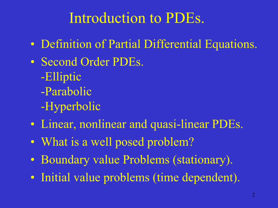
Introduction to PDEs.• Definition of Partial Differential Equations.• Second Order PDEs.

-Elliptic-Parabolic-Hyperbolic

• Linear, nonlinear and quasi-linear PDEs.• What is a well posed problem?• Boundary value Problems (stationary).• Initial value problems (time dependent).

3

Differential Equations

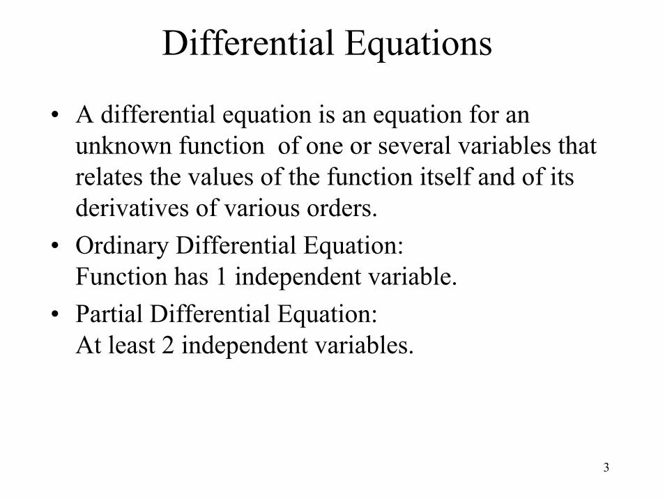
• A differential equation is an equation for an unknown function of one or several variables that relates the values of the function itself and of its derivatives of various orders.

• Ordinary Differential Equation:Function has 1 independent variable.

• Partial Differential Equation:At least 2 independent variables.

4

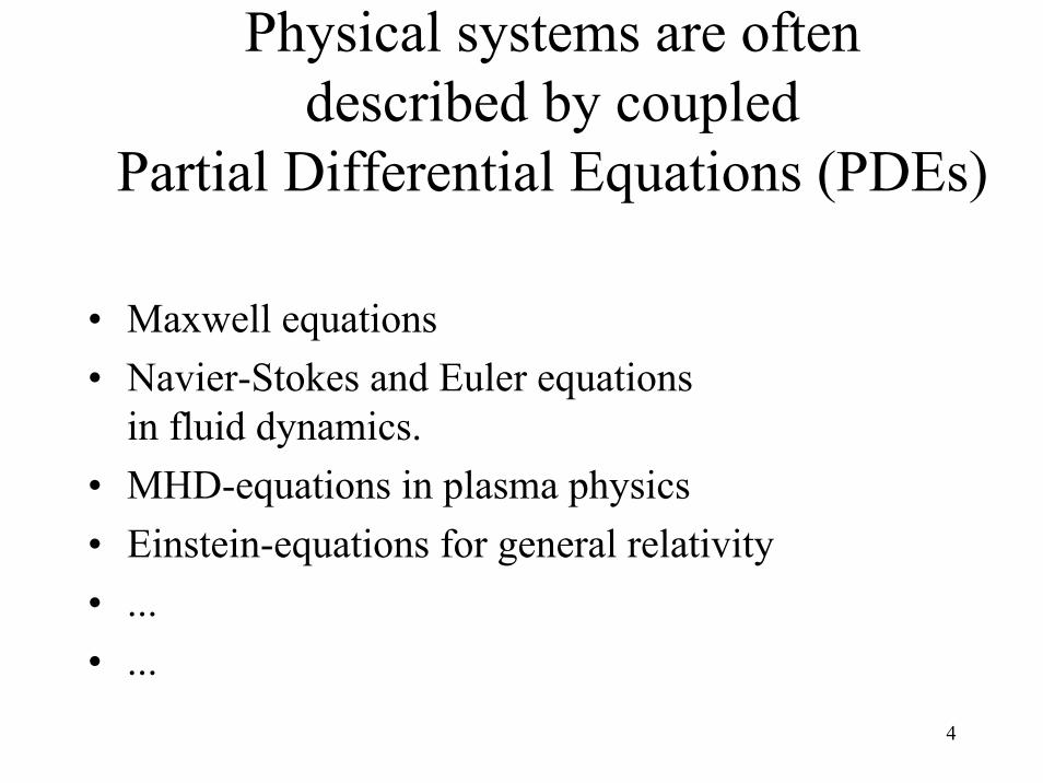
Physical systems are oftendescribed by coupled

Partial Differential Equations (PDEs)

• Maxwell equations• Navier-Stokes and Euler equations

in fluid dynamics.• MHD-equations in plasma physics• Einstein-equations for general relativity• ...• ...

5

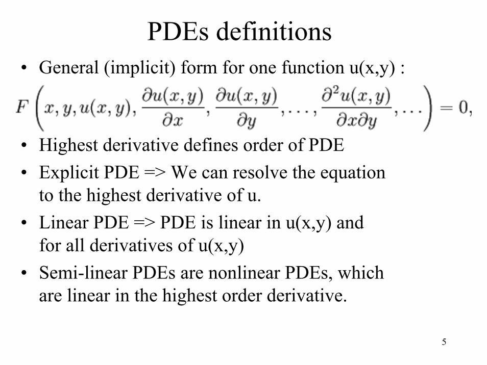
PDEs definitions• General (implicit) form for one function u(x,y) :

• Highest derivative defines order of PDE• Explicit PDE => We can resolve the equation

to the highest derivative of u. • Linear PDE => PDE is linear in u(x,y) and

for all derivatives of u(x,y)• Semi-linear PDEs are nonlinear PDEs, which

are linear in the highest order derivative.

6

Linear PDEs of 2. Order

• a(x,y)c(x,y) − b(x,y)2 / 4 > 0 Elliptic• a(x,y)c(x,y) − b(x,y)2 / 4 = 0 Parabolic• a(x,y)c(x,y) − b(x,y)2 / 4 < 0 Hyperbolic

Quasi-linear: coefficients depend on u and/orfirst derivative of u, but NOT on second derivatives.

7

PDEs and Quadratic Equations

• Quadratic equations in the form

describe cone sections.

• a(x,y)c(x,y) − b(x,y)2 / 4 > 0 Ellipse• a(x,y)c(x,y) − b(x,y)2 / 4 = 0 Parabola• a(x,y)c(x,y) − b(x,y)2 / 4 < 0 Hyperbola

8

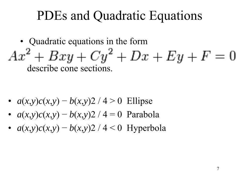
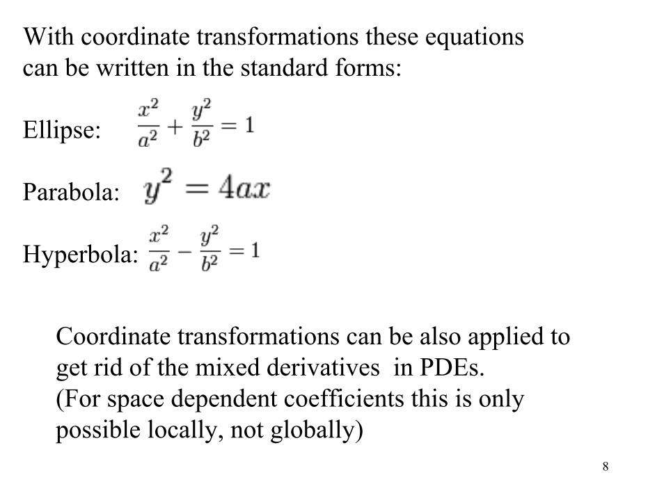
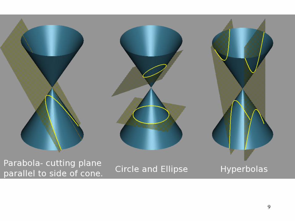
With coordinate transformations these equations can be written in the standard forms:

Ellipse:

Parabola:

Hyperbola:

Coordinate transformations can be also applied toget rid of the mixed derivatives in PDEs.(For space dependent coefficients this is only possible locally, not globally)

9

10

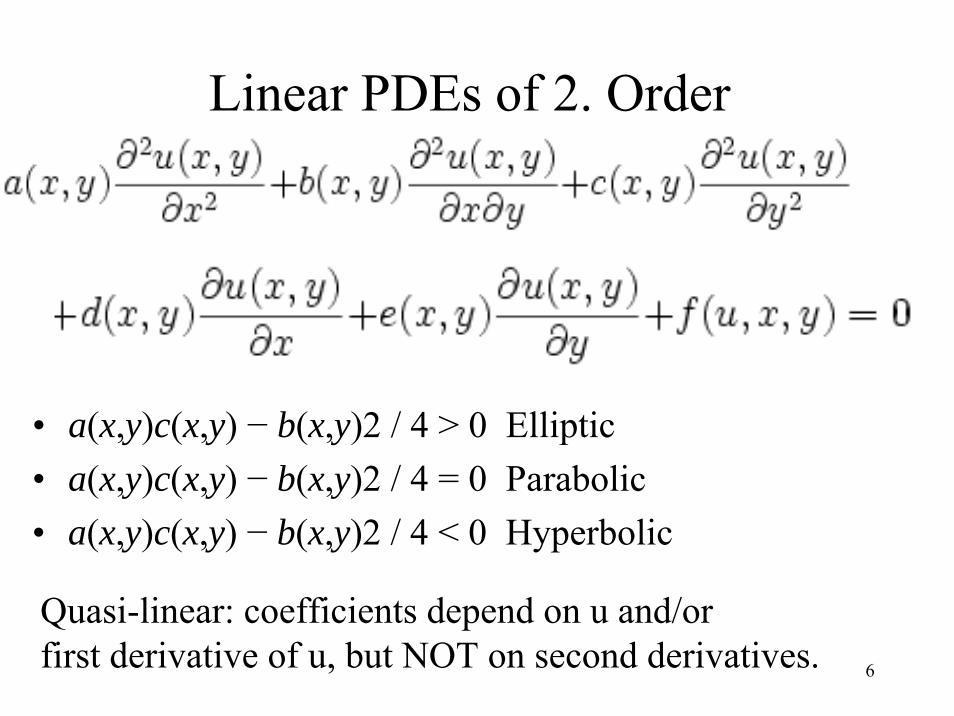
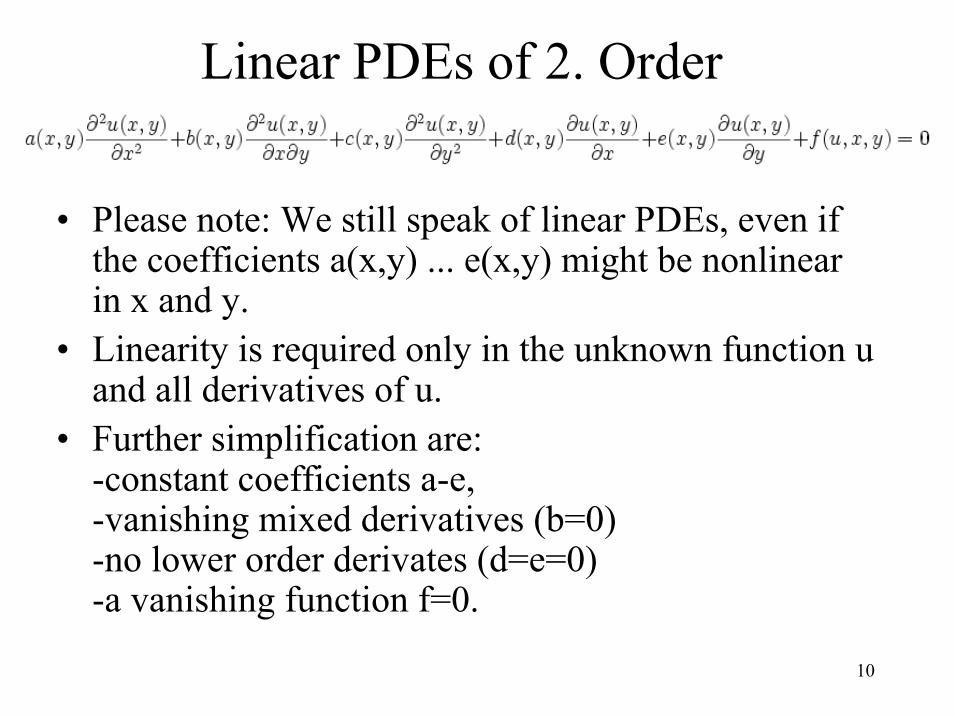
Linear PDEs of 2. Order

• Please note: We still speak of linear PDEs, even ifthe coefficients a(x,y) ... e(x,y) might be nonlinearin x and y.

• Linearity is required only in the unknown function u and all derivatives of u.

• Further simplification are:-constant coefficients a-e,-vanishing mixed derivatives (b=0) -no lower order derivates (d=e=0) -a vanishing function f=0.

11

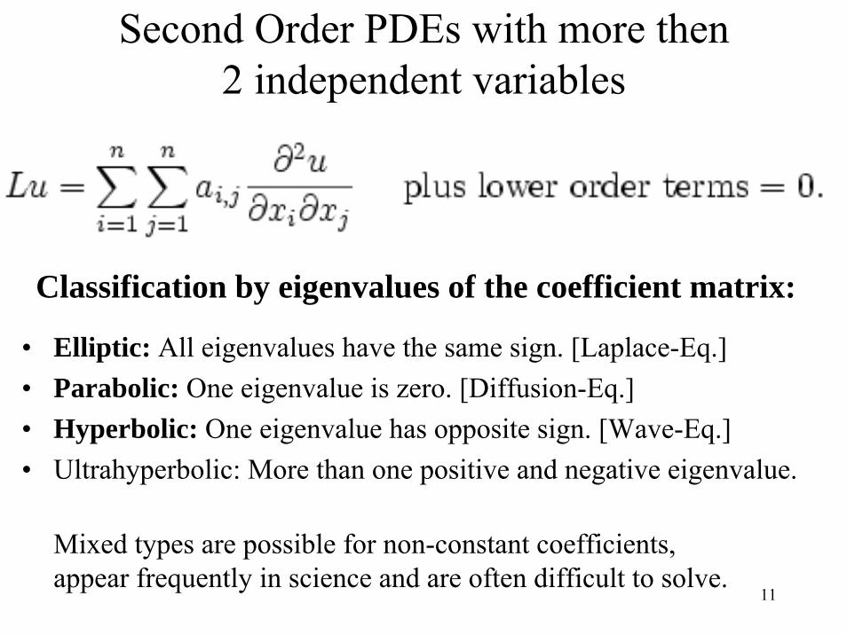
Second Order PDEs with more then2 independent variables

• Elliptic: All eigenvalues have the same sign. [Laplace-Eq.]• Parabolic: One eigenvalue is zero. [Diffusion-Eq.]• Hyperbolic: One eigenvalue has opposite sign. [Wave-Eq.]• Ultrahyperbolic: More than one positive and negative eigenvalue.

Mixed types are possible for non-constant coefficients,appear frequently in science and are often difficult to solve.

Classification by eigenvalues of the coefficient matrix:

12

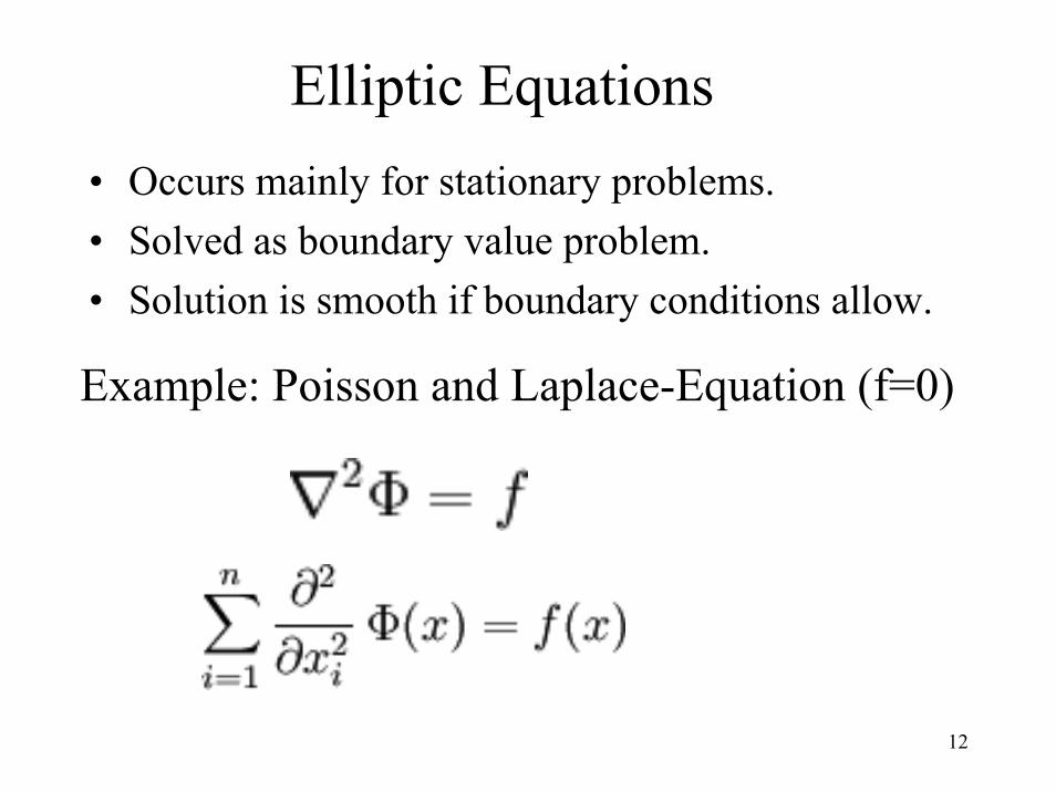
Elliptic Equations• Occurs mainly for stationary problems.• Solved as boundary value problem.• Solution is smooth if boundary conditions allow.

Example: Poisson and Laplace-Equation (f=0)

13

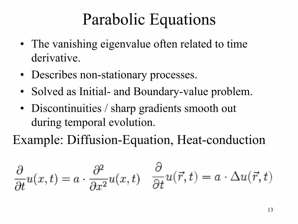
Parabolic Equations• The vanishing eigenvalue often related to time

derivative.• Describes non-stationary processes.• Solved as Initial- and Boundary-value problem.• Discontinuities / sharp gradients smooth out

during temporal evolution.Example: Diffusion-Equation, Heat-conduction

14

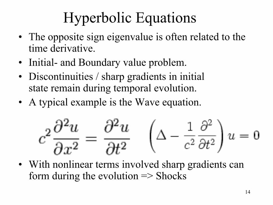
Hyperbolic Equations• The opposite sign eigenvalue is often related to the

time derivative.• Initial- and Boundary value problem.• Discontinuities / sharp gradients in initial

state remain during temporal evolution.• A typical example is the Wave equation.

• With nonlinear terms involved sharp gradients can form during the evolution => Shocks

15

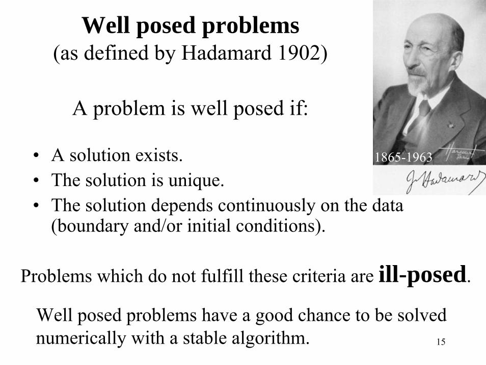
Well posed problems(as defined by Hadamard 1902)

A problem is well posed if:

• A solution exists.• The solution is unique.• The solution depends continuously on the data

(boundary and/or initial conditions).

Problems which do not fulfill these criteria are ill-posed.

Well posed problems have a good chance to be solvednumerically with a stable algorithm.

1865-1963

16

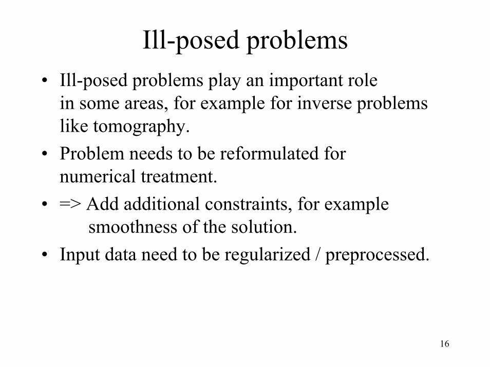
Ill-posed problems• Ill-posed problems play an important role

in some areas, for example for inverse problems like tomography.

• Problem needs to be reformulated fornumerical treatment.

• => Add additional constraints, for examplesmoothness of the solution.

• Input data need to be regularized / preprocessed.

17

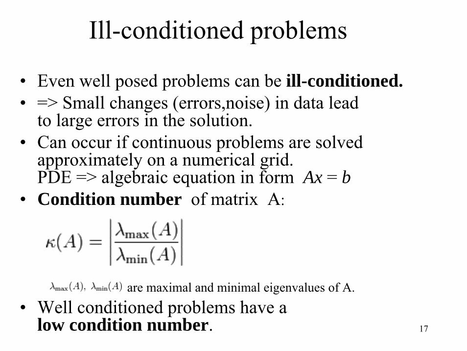
Ill-conditioned problems

• Even well posed problems can be ill-conditioned. • => Small changes (errors,noise) in data lead

to large errors in the solution.• Can occur if continuous problems are solved

approximately on a numerical grid.PDE => algebraic equation in form Ax = b

• Condition number of matrix A:

are maximal and minimal eigenvalues of A.

• Well conditioned problems have a low condition number.

18

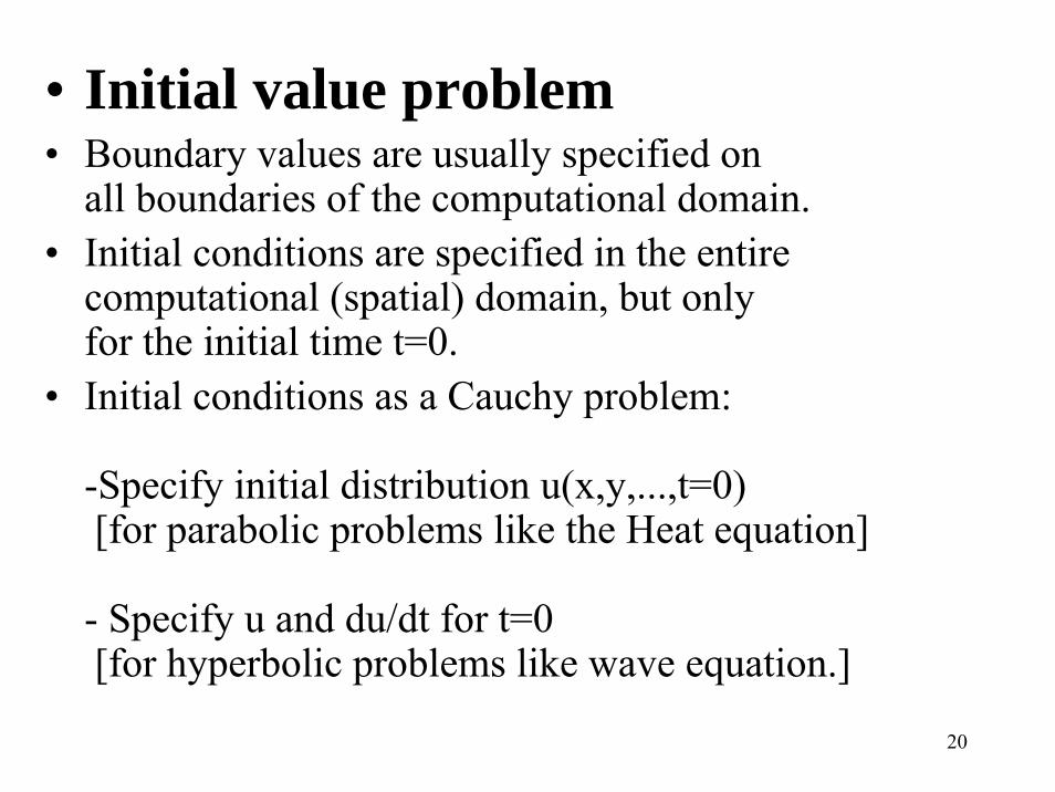
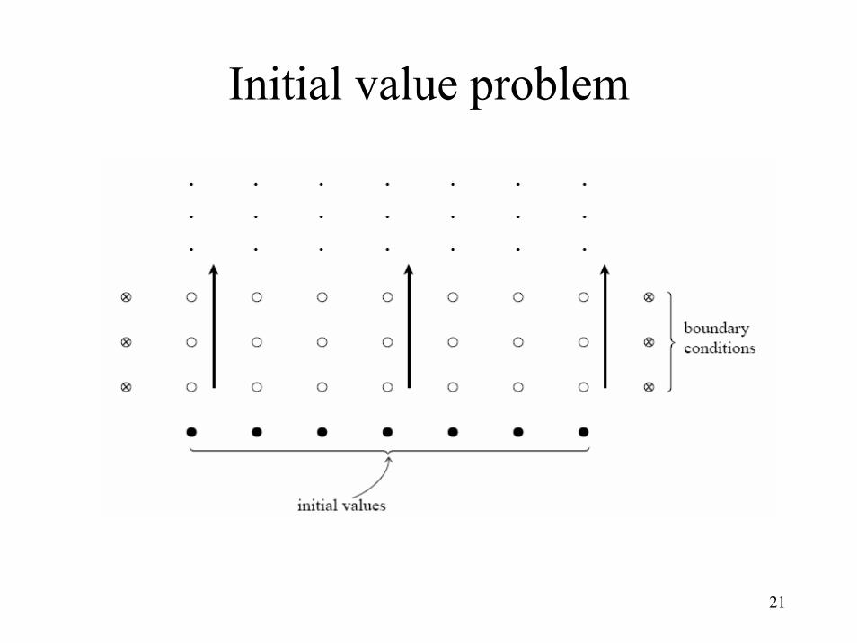
How to solve PDEs?• PDEs are solved together with appropriate

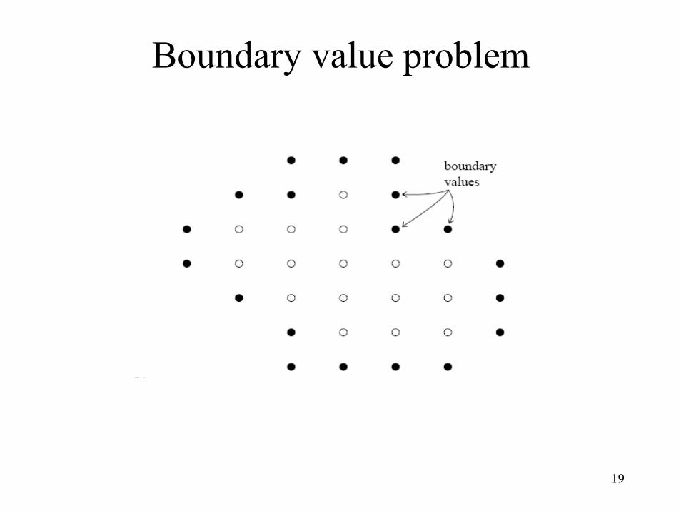
Boundary Conditions and/or Initial Conditions.• Boundary value problem

-Dirichlet B.C.: Specify u(x,y,...) on boundaries(say at x=0, x=Lx, y=0, y=Ly in a rectangular box)-von Neumann B.C.: Specify normal gradient ofu(x,y,...) on boundaries.

In principle boundary can be arbitrary shaped.(but difficult to implement in computer codes)

19

Boundary value problem

20

• Initial value problem• Boundary values are usually specified on

all boundaries of the computational domain.• Initial conditions are specified in the entire

computational (spatial) domain, but onlyfor the initial time t=0.

• Initial conditions as a Cauchy problem:

-Specify initial distribution u(x,y,...,t=0)[for parabolic problems like the Heat equation]

- Specify u and du/dt for t=0[for hyperbolic problems like wave equation.]

21

Initial value problem

22

Cauchy Boundary conditions• Cauchy B.C. impose both Dirichlet

and Von Neumann B.C. on part ofthe boundary (for PDEs of 2. order).

• More general: For PDEs of order n theCauchy problem specifies u and allderivatives of u, up to the order n-1on parts of the boundary.

• In physics the Cauchy problem is oftenrelated to temporal evolution problems (initial conditions specified for t=0)

Augustin Louis Cauchy1789-1857

23

Introduction to PDEsSummary

• What is a well posed problem? Solution exists, is unique, continuous on boundary conditions.

• Elliptic (Poisson), Parabolic (Diffusion)and Hyperbolic (Wave) PDEs.

• PDEs are solved with boundary conditionsand initial conditions.

• What are Dirichlet and von Neumannboundary conditions?

24

Numerical Integration ofPartial Differential Equations (PDEs)

••• Introduction to Introduction to Introduction to PDEsPDEsPDEs...• Semi-analytic methods to solve PDEs.••• Introduction to Finite Differences.Introduction to Finite Differences.Introduction to Finite Differences.••• Stationary Problems, Elliptic Stationary Problems, Elliptic Stationary Problems, Elliptic PDEsPDEsPDEs...••• Time dependent Problems.Time dependent Problems.Time dependent Problems.••• Complex Problems in Solar System Complex Problems in Solar System Complex Problems in Solar System

Research.Research.Research.

25

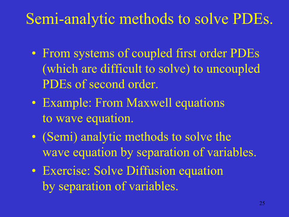
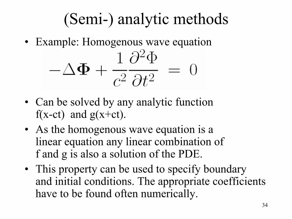
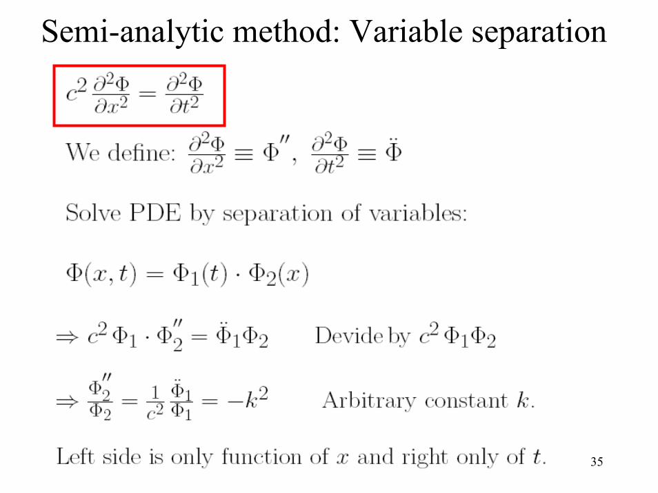
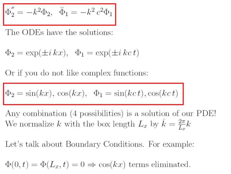
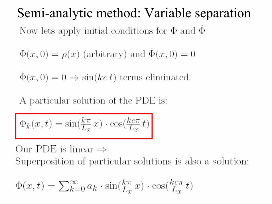
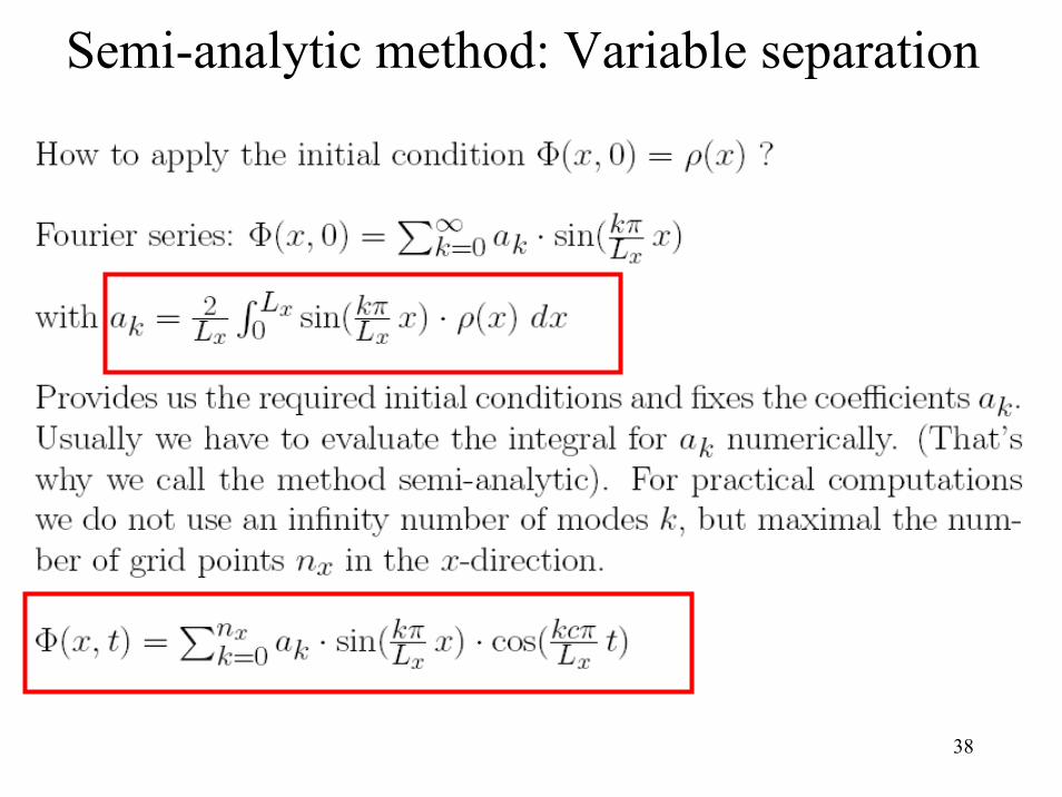
Semi-analytic methods to solve PDEs.

• From systems of coupled first order PDEs(which are difficult to solve) to uncoupledPDEs of second order.

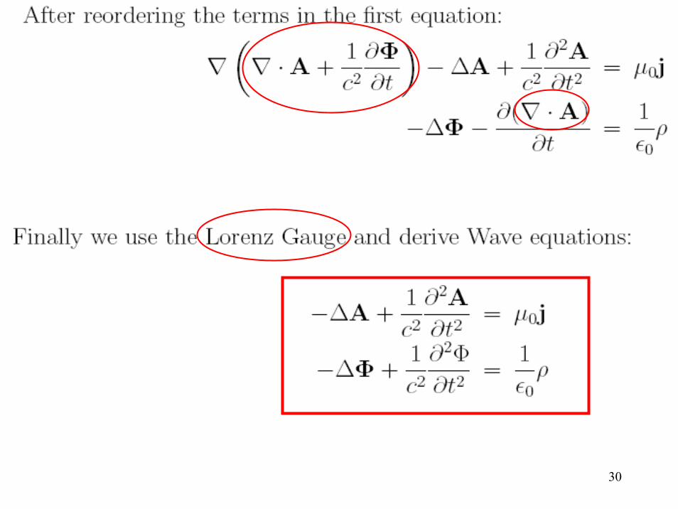
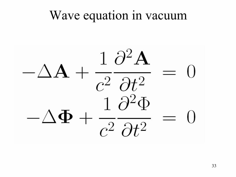
• Example: From Maxwell equationsto wave equation.

• (Semi) analytic methods to solve thewave equation by separation of variables.

• Exercise: Solve Diffusion equationby separation of variables.

26

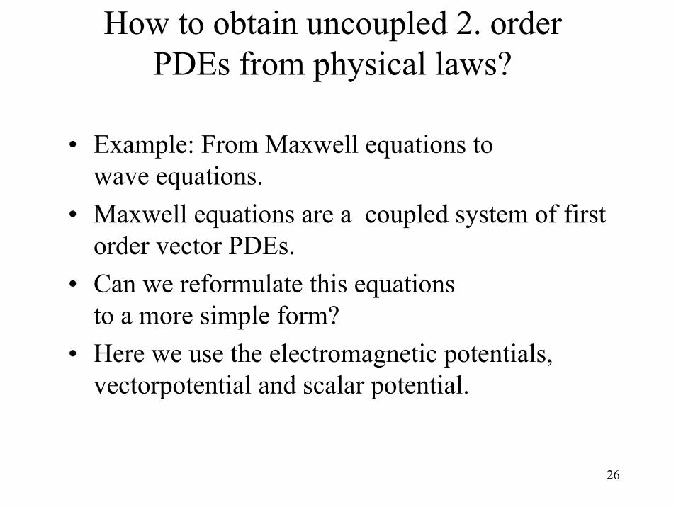
How to obtain uncoupled 2. orderPDEs from physical laws?

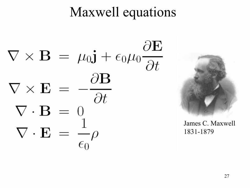
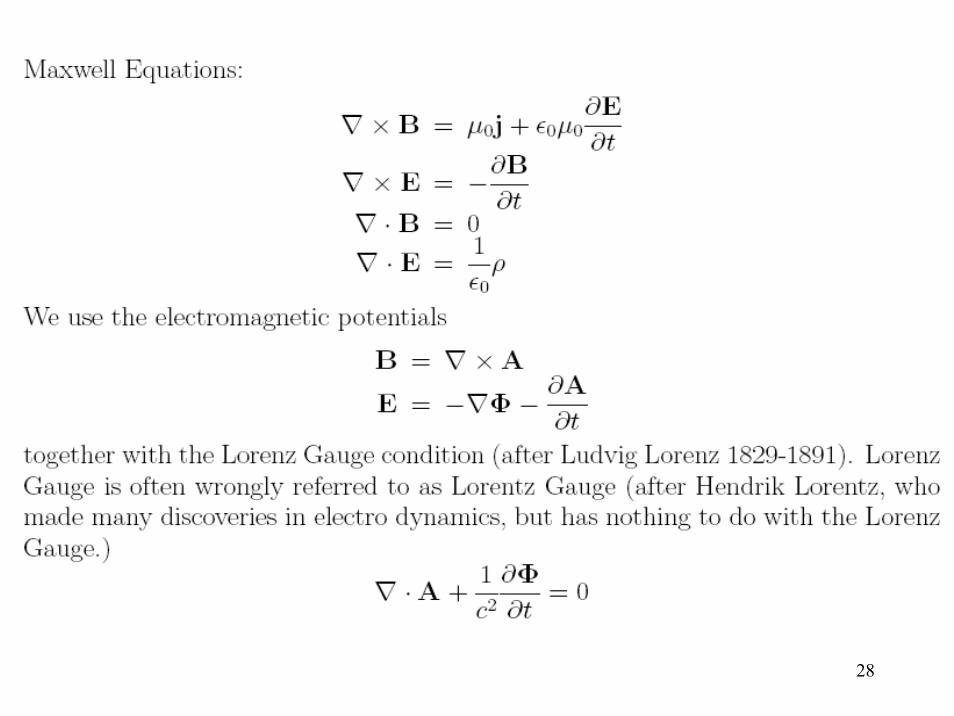
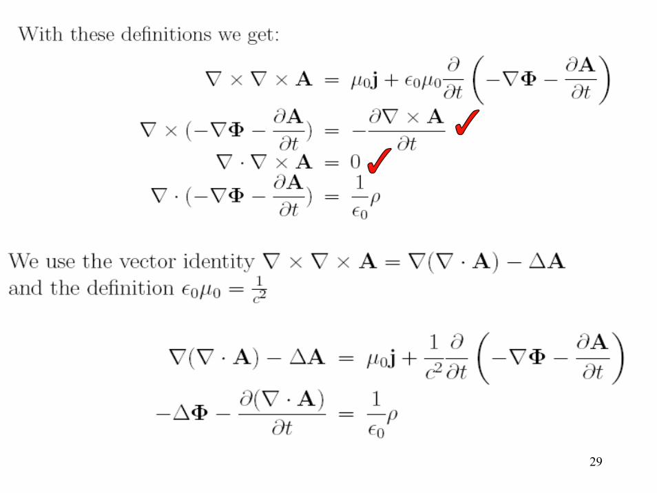
• Example: From Maxwell equations to wave equations.

• Maxwell equations are a coupled system of first order vector PDEs.

• Can we reformulate this equationsto a more simple form?

• Here we use the electromagnetic potentials,vectorpotential and scalar potential.

27

Maxwell equations

James C. Maxwell1831-1879

28

29

30

31

What do we win with wave equations?

• Inhomogenous coupled system ofMaxwell reduces to wave equations.

• We get 2. order scalar PDEsfor components of electric andmagnetic potentials.

• Equation are not coupled and havesame form.

• Well known methods exist to solvethese wave equations.

32

Wave equation

• Electric charges and currents on right side ofwave-equation can be computed from other sources:

• Moments of electron and ion-distribution inspace-plasma.

• The particle-distributions can be derived fromnumerical simulations, e.g. by solving theVlasov equation for each species.

• Here we study the wave equation in vacuum forsimplicity.

33

Wave equation in vacuum

34

(Semi-) analytic methods• Example: Homogenous wave equation

• Can be solved by any analytic function f(x-ct) and g(x+ct).

• As the homogenous wave equation is alinear equation any linear combination off and g is also a solution of the PDE.

• This property can be used to specify boundaryand initial conditions. The appropriate coefficientshave to be found often numerically.

35

Semi-analytic method: Variable separation

36

37

Semi-analytic method: Variable separation

38

Semi-analytic method: Variable separation

39

Show: demo_wave_sep.pro

This is an IDL-program toanimate the wave-equation

Semi-analytic method: Variable separation

40

Exercise:1D diffusion equation

lecture_diffusion_draft.proThis is a draft IDL-program to solve the diffusion equation by separation of variables.

Task: Find separable solutions forDirichlet and von Neumann boundary conditionsand implement them.

41

Semi-analytic methods Summary

• Some (mostly) linear PDEs with constantcoefficients can be solved analytically.

• One possibility is the method ‘Separation of variables’, which leads toordinary differential equations.

• For linear PDEs.: Superposition of different solutions is also a solution of the PDE.

42

Numerical Integration ofPartial Differential Equations (PDEs)

••• Introduction to Introduction to Introduction to PDEsPDEsPDEs...••• SemiSemiSemi---analytic methods to solve analytic methods to solve analytic methods to solve PDEsPDEsPDEs...• Introduction to Finite Differences.••• Stationary Problems, Elliptic Stationary Problems, Elliptic Stationary Problems, Elliptic PDEsPDEsPDEs...••• Time dependent Problems.Time dependent Problems.Time dependent Problems.••• Complex Problems in Solar System Complex Problems in Solar System Complex Problems in Solar System

Research.Research.Research.

43

Introduction to Finite Differences.• Remember the definition of the

differential quotient.• How to compute the differential quotient

with a finite number of grid points?• First order and higher order approximations.• Central and one-sided finite differences.• Accuracy of methods for smooth

and not smooth functions.• Higher order derivatives.

44

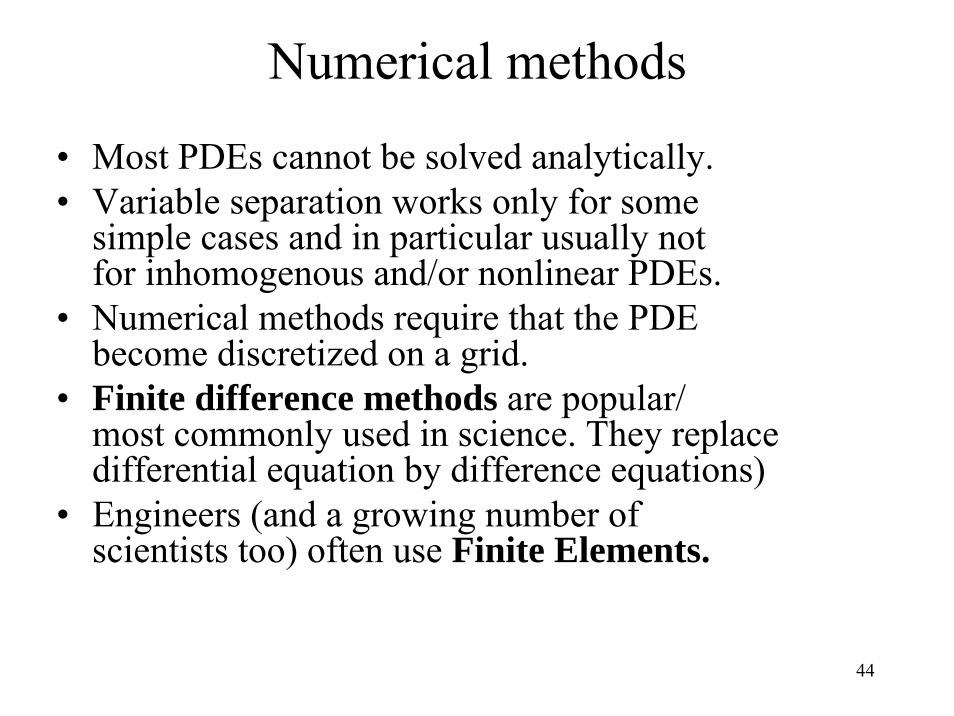
Numerical methods

• Most PDEs cannot be solved analytically.• Variable separation works only for some

simple cases and in particular usually notfor inhomogenous and/or nonlinear PDEs.

• Numerical methods require that the PDEbecome discretized on a grid.

• Finite difference methods are popular/most commonly used in science. They replace differential equation by difference equations)

• Engineers (and a growing number ofscientists too) often use Finite Elements.

45

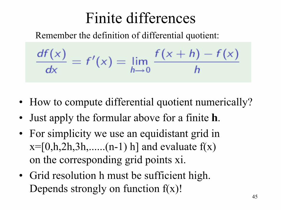
Finite differences

• How to compute differential quotient numerically?• Just apply the formular above for a finite h.• For simplicity we use an equidistant grid in

x=[0,h,2h,3h,......(n-1) h] and evaluate f(x)on the corresponding grid points xi.

• Grid resolution h must be sufficient high.Depends strongly on function f(x)!

Remember the definition of differential quotient:

46

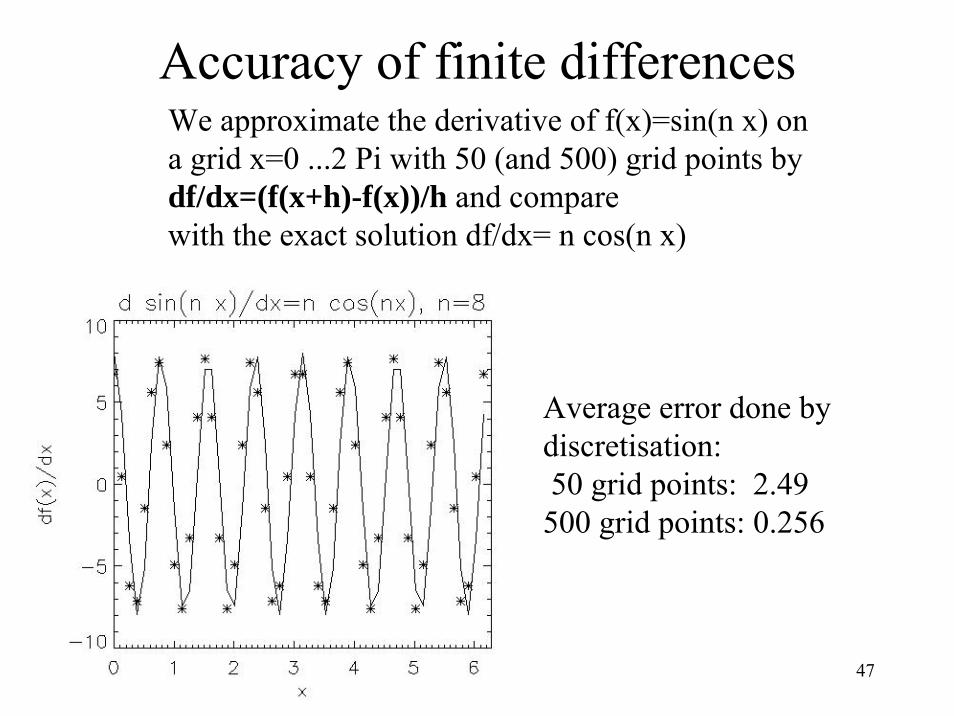
Accuracy of finite differencesWe approximate the derivative of f(x)=sin(n x) ona grid x=0 ...2 Pi with 50 (and 500) grid points by df/dx=(f(x+h)-f(x))/h and comparewith the exact solution df/dx= n cos(n x)

Average error done by discretisation: 50 grid points: 0.040 500 grid points: 0.004

47

Accuracy of finite differencesWe approximate the derivative of f(x)=sin(n x) ona grid x=0 ...2 Pi with 50 (and 500) grid points by df/dx=(f(x+h)-f(x))/h and comparewith the exact solution df/dx= n cos(n x)

Average error done by discretisation: 50 grid points: 2.49 500 grid points: 0.256

48

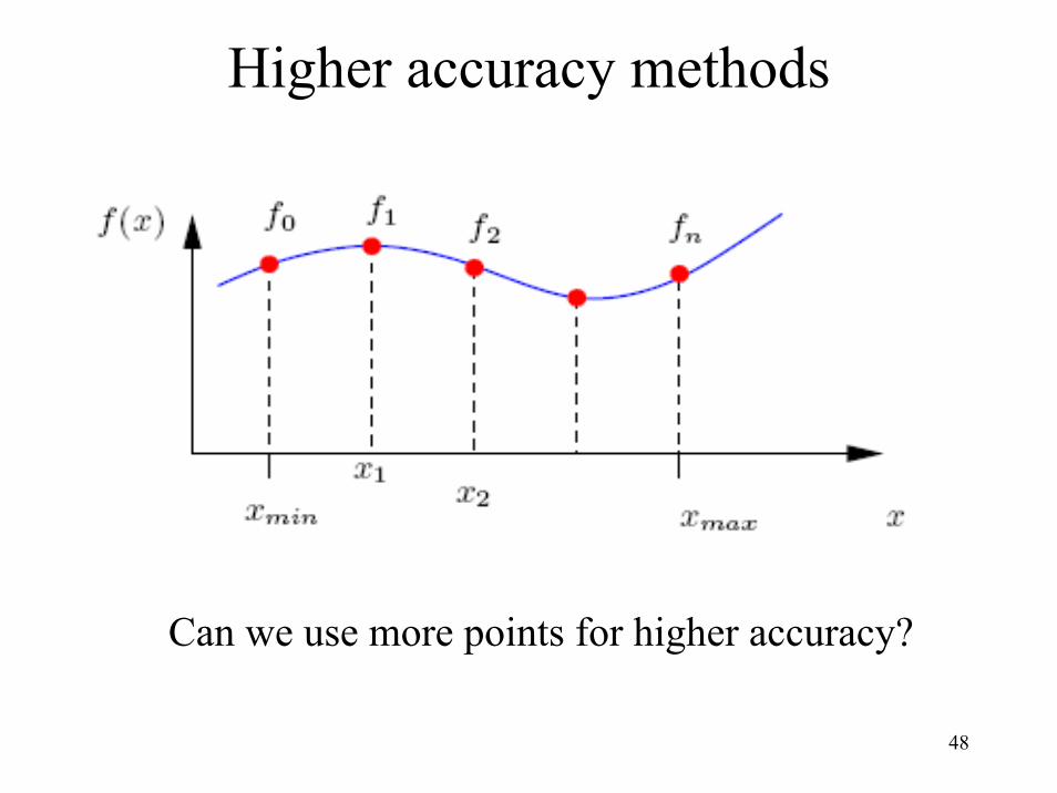
Higher accuracy methods

Can we use more points for higher accuracy?

49

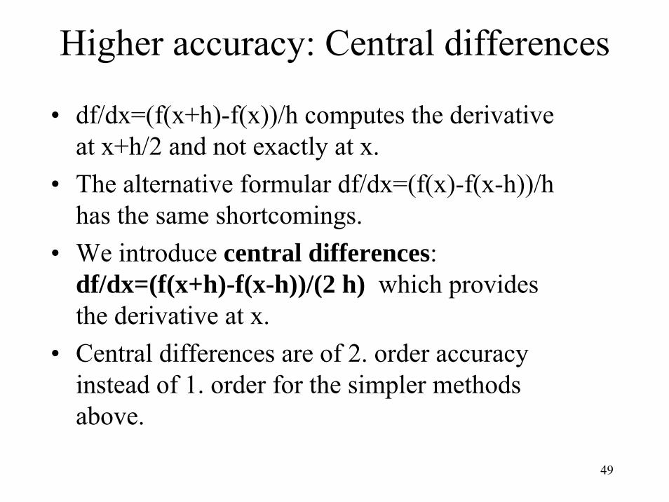
Higher accuracy: Central differences

• df/dx=(f(x+h)-f(x))/h computes the derivativeat x+h/2 and not exactly at x.

• The alternative formular df/dx=(f(x)-f(x-h))/hhas the same shortcomings.

• We introduce central differences:df/dx=(f(x+h)-f(x-h))/(2 h) which providesthe derivative at x.

• Central differences are of 2. order accuracyinstead of 1. order for the simpler methodsabove.

50

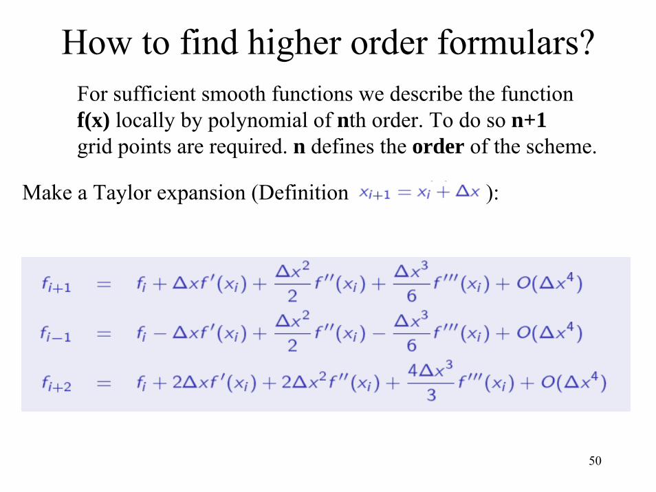
How to find higher order formulars?For sufficient smooth functions we describe the functionf(x) locally by polynomial of nth order. To do so n+1grid points are required. n defines the order of the scheme.

Make a Taylor expansion (Definition ):

51

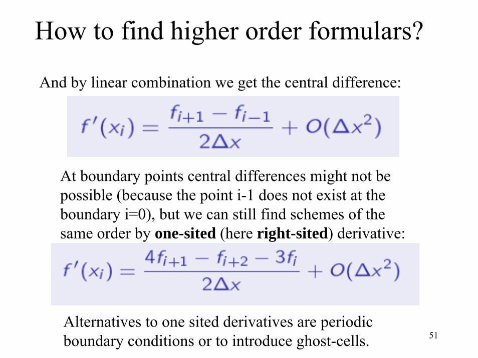
How to find higher order formulars?

And by linear combination we get the central difference:

At boundary points central differences might not bepossible (because the point i-1 does not exist at theboundary i=0), but we can still find schemes of thesame order by one-sited (here right-sited) derivative:

Alternatives to one sited derivatives are periodicboundary conditions or to introduce ghost-cells.

52

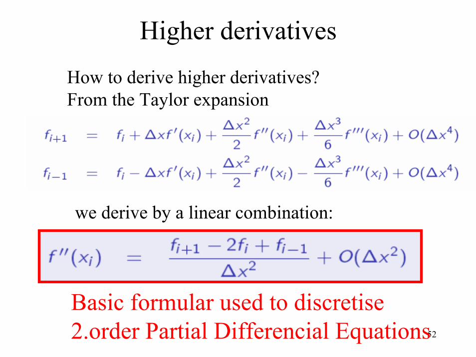
Higher derivatives

How to derive higher derivatives?From the Taylor expansion

we derive by a linear combination:

Basic formular used to discretise2.order Partial Differencial Equations

53

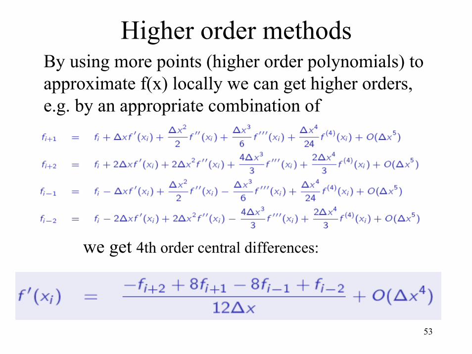
Higher order methodsBy using more points (higher order polynomials) toapproximate f(x) locally we can get higher orders,e.g. by an appropriate combination of

we get 4th order central differences:

54

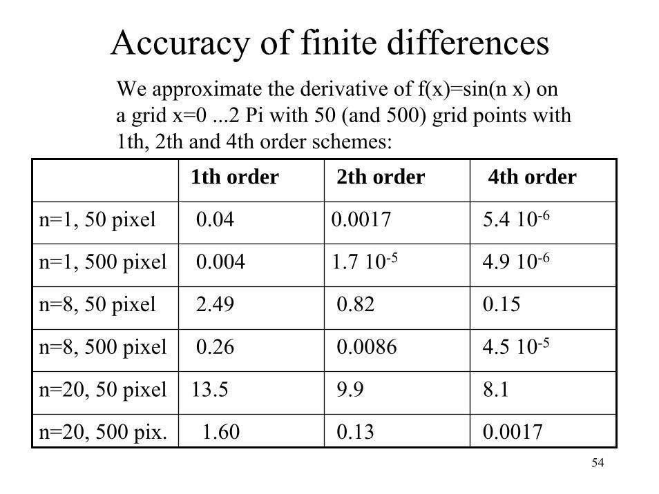
Accuracy of finite differencesWe approximate the derivative of f(x)=sin(n x) ona grid x=0 ...2 Pi with 50 (and 500) grid points with1th, 2th and 4th order schemes:

1th order 2th order 4th order

n=1, 50 pixel 0.04 0.0017 5.4 10-6

n=1, 500 pixel 0.004 1.7 10-5 4.9 10-6

n=8, 50 pixel 2.49 0.82 0.15

n=8, 500 pixel 0.26 0.0086 4.5 10-5

n=20, 50 pixel 13.5 9.9 8.1

n=20, 500 pix. 1.60 0.13 0.0017

55

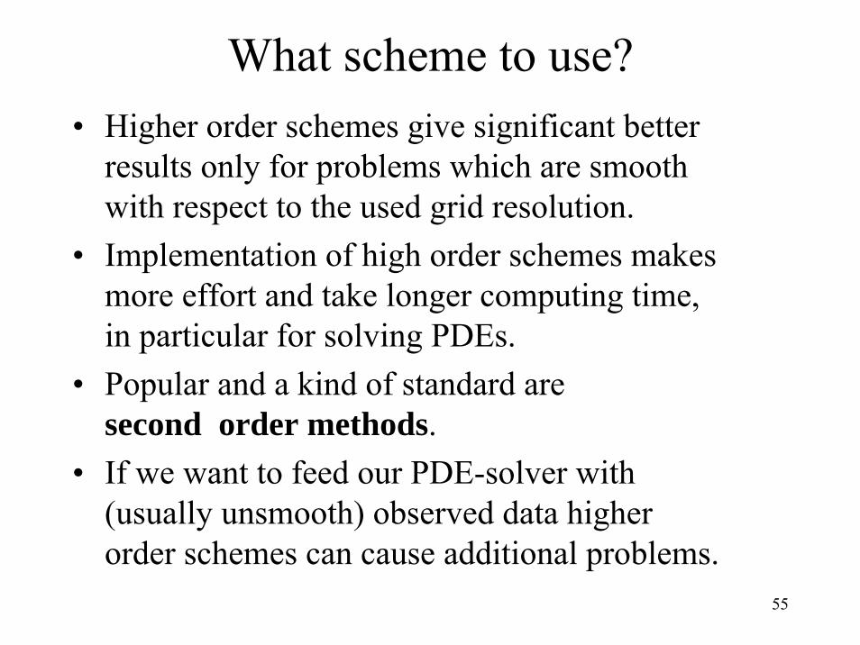
What scheme to use?• Higher order schemes give significant better

results only for problems which are smoothwith respect to the used grid resolution.

• Implementation of high order schemes makes more effort and take longer computing time,in particular for solving PDEs.

• Popular and a kind of standard are second order methods.

• If we want to feed our PDE-solver with (usually unsmooth) observed data higherorder schemes can cause additional problems.

56

Finite differences Summary

• Differential quotient is approximated by finite differences on a discrete numerical grid.

• Popular are in particular central differences,which are second order accurate.

• The grid resolution should be high enough, sothat the discretized functions appear smooth.=> Physical gradients should be on larger scales as the grid resolution.