19
Numerical integration on trimmed three-dimensional domains Felix Scholz, Bert J¨ uttler G+S Report No. 85 May 2019

Numerical integration on
trimmed three-dimensional
domains
Felix Scholz, Bert Juttler
G+S Report No. 85
May 2019

Numerical integration on trimmed three-dimensional domains
Felix Scholza, Bert Juttlera,b
aRadon Institute for Computational and Applied Mathematics (RICAM), Austrian Academy of Sciences, Linz,Austria
bInstitute of Applied Geometry, Johannes Kepler University Linz, Austria
Abstract
We present a novel technique for the numerical integration of trivariate functions on trimmeddomains. Our approach combines a linear approximation of the trimming surface with a correctionterm. The latter term makes it possible to achieve a cubic convergence rate, which is one orderhigher than the rate obtained by using the linear approximation only. We also present numericalexperiments that demonstrate the method’s potential for applications in isogeometric analysis.
Keywords: Trimming, isogeometric analysis, numerical integration, quadrature
1. Introduction
The flexibility of NURBS surface representations in computer-aided design is greatly enhancedby the use of trimming. More precisely, only a part of the parameter domain is active, while aregion defined by a trimming curve is discarded. For example, the trimming curve can be theresult of a surface-surface intersection.
Isogeometric analysis [1, 2] is based on the use of bi- and trivariate NURBS parameterizationsof two- and three-dimensional computational domains. Again, the use of trimming operationsincreases the flexibility of these representations of the geometry. According to the isogeometricparadigm, the same discrete space is employed for the analysis (i.e. the numerical solution ofpartial differential equations) as for the representation of the geometry, thus unifying the fields ofcomputer-aided design and numerical simulation.
Trimming also plays a role in the context of unfitted finite element methods [3], such as thefinite cell method [4]. In this class of methods, the solution is approximated using a backgroundfinite element mesh that is intersected with the underlying geometry.
In both situations, efficient and accurate quadrature rules are needed to perform numericalintegration on the trimmed elements of the discretization spaces. They are required in orderto assemble the Galerkin matrices as well as the right-hand sides (load vectors) of the discretesystems.
Several approaches to numerical integration on trimmed domains have been considered. Mostof this earlier work is limited to the two-dimensional case, see [5] and the references therein. Wediscuss a number of related results, focusing on the trivariate case:
A common approach for numerical quadrature on trimmed domains is to subdivide the trimmedelements into simpler objects, which is sometimes called untrimming, and to find local approxima-tions that can be dealt with by high-order quadrature rules. The accuracy of the overall procedureis then governed by the geometric approximation error.
In the volumetric case, this has been described in [6], where the trimming surface is approxi-mated by piece-wise polynomials, and in [7], using a marching cube-type approach. Tetrahedralelements have also been used for the discretization of partial differential equations on trimmedvolumes [8]. In [9], the trimmed patch is subdivided into a number of singular tensor-productB-Spline patches whose boundaries approximate the trimming surface.
Email addresses: [email protected] (Felix Scholz), [email protected] (Bert Juttler)
NFN S117 Technical Report May 8, 2019

Clearly, the success of these approaches depends on the ability to compute surface-surfaceintersections, which is well-known to be a delicate problem [10]. Among other approaches, the useof interval arithmetics has been proposed to achieve robustness in degenerate or nearly-degeneratesituations [11].
In the context of the finite cell method, the smart octree method for quadrature on volumetricdomains has been introduced in [12]. It is based on an extended adaptive subdivision of theelements into octants. More precisely, the octant nodes are moved to the trimming surface, inorder to increase the accuracy of the result.
An interesting approach has been presented in [13], where the authors show how to constructa specific quadrature rule for each trimmed element with the help of non-linear optimization. Asa prerequisite, the method evaluates the integrals of polynomials on a piece-wise linear approxi-mation to the trimmed domain using a subdivision into convex subdomains, and this determinesthe overall accuracy. The numerical experiments demonstrate that the method is suitable fortwo-dimensional problems.
Finally, we note that several techniques exist that can help to avoid trimming. Besides untrim-ming, these include discontinuous Galerkin methods on overlapping patches [14], Schwarz-typedomain decomposition methods [15, 16].
The present paper builds on results from [17], where we presented a method for the quadratureon trimmed two-dimensional domains with an implicitly defined trimming function. The trimmingfunction is locally approximated by a linear function whose level-set is used for an initial approx-imation of the integral. It is shown that the approximation order of the resulting quadrature rulecan be increased by adding an error correction term based on a Taylor expansion.
We generalize this idea to the case of trimmed volumetric domains. Again, we assume thatthe trimming surface is given implicitly as a level set of a function, for example as the result ofa Boolean operation on two domains. For parametric trimming surfaces, exact or approximateimplicitization [18, 19] has to be applied as a preprocessing step.
The trivariate trimming function is approximated by a linear function using constrained leastsquares optimization, thereby ensuring a consistent topology. The resulting quadratic order ofconvergence of the quadrature rule is then increased by adding a simple error correction term. Sincethis error correction term only consists of a bivariate integral, it preserves the overall computationalcomplexity, making the method very efficient.
We apply our method to the problems of L2-projection and isogeometric analysis on trimmedvolumes. In addition to the numerical quadrature, another challenge lies in the stability of thetrimmed basis functions. If one uses the standard B-Spline basis, restricted to the trimmed domain,the supports of the basis function may be arbitrarily small, resulting in a loss of stability. Thisinstability can be addressed using modified bases such as extended B-Splines [20, 21] or immersedB-Splines [22]. Other approaches are the addition of a stabilization term (ghost penalty) to thebilinear form [23] and the omission of basis functions with sufficiently small support [24]. Inour numerical examples, we implemented the extended B-Spline basis, which recovers stabilityby eliminating unstable functions and adding them to a number of stable ones with appropriateweights, such that the approximation power stays the same.
The paper is organized as follows: We first state the considered problem in Section 2. Then wedescribe the reduction to base cases that our method can handle in Section 3. We introduce thelinearized trimmed quadrature rule in Section 4 and its extension using the first order correctionterm in Section 5. Finally, we present numerical examples for the quadrature and its applicationto L2-projection and isogeometric analysis in Section 6.
2. Problem
Given smooth trivariate functions f and τ and an axis-aligned box B ⊂ R3, we develop amethod for the numerical evaluation of the integral
Iτf =
∫
Bτ
f(x, y, z) dz dy dx
2

over the part of B where τ , which is called the trimming function, takes positive values,
Bτ = (x, y, z) ∈ B : τ(x, y, z) > 0.
More precisely, we approximate the exact integral by using a weighted quadrature rule
Qτf =∑
i
wif(xi, yi, zi) ≈ Iτf
with quadrature nodes (xi, yi, zi) and weights wi.Our approach generalizes earlier work on the two-dimensional case [17]. It consists of three
main steps:
1. We subdivide B into smaller boxes until the sign distribution of the trimming function τ atthe boxes’ vertices is an instance of one of seven base cases.
2. We approximate the trimming function τ by a linear polynomial σ and perform an approx-imate evaluation of the integral
Iσf =
∫
Bσ
f(x, y, z) dz dy dx
by Gauss quadrature.
3. We improve this initial approximation to Iτf by adding an error correction term that isderived from the Taylor expansion of the linear interpolant Iσ+u(τ−σ)f at u = 0. Thisresults in a bivariate integral, which is again evaluated via Gauss quadrature.
Summing up, the quadrature rule Qτ consists of two types of quadrature nodes and weights in eachcell: the nodes and weights of the trivariate Gauss quadrature performed in the second step andthe nodes and weights of the bivariate Gauss quadrature needed to evaluate the error correctionterm in the third step.
The next three sections discuss the three steps in more detail.
3. Subdivision and base cases
Our method is designed to be able to treat a number of base cases, which are characterizedby the sign distribution of the trimming function on the vertices of B. Intuitively, the signdistribution captures how the trimming surface cuts the box B. In addition, we only treat boxes,whose maximum edge length does not exceed a user-defined constant h, in order to maintain theaccuracy of the numerical integration.
If we distinguish between positive and non-positive signs of τ at the vertices of B, we arrive at28 = 256 possible cases. However, this number can be reduced significantly by considering the 48isometries of the cube (i.e. the rotations and reflections of the cell) and possibly inverting the signsof τ at the vertices. This results in the 15 cube configurations of the marching cube algorithm.
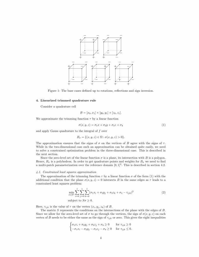
Five of these configurations, which are shown in Figure 1, correspond to a single componentof the trimming surface within B. More precisely, if the trimming surface has a single componentwithin B, then the sign distribution belongs to one of these configurations. These are the basecases of our method, which are handled directly. In addition we also handle the case of onlypositive signs, which corresponds to an untrimmed box B = Bτ . Clearly, this case does notrequire any particular treatment, simple Gauss quadrature is sufficient.
The remaining nine configurations are dealt with by splitting the box B into eight sub-boxes.The splitting is applied recursively until each generated box is an instance of one of the six basecases. Similarly, we split the box B into eight sub-boxes if the maximum edge length exceedsh. The total number of generated boxes satisfies Nh = O( 1
h3 ) if the trimming surface is regularwithin B.
It should be noted that the trimming surface may possess several components within B evenif the sign distribution belongs to one of the base cases. As we shall see later, our technique givescorrect results also in these situations.
3
+ +
+ +
− −
− −
+ −
− −
− −
− −
+ −
+ −
− −
− −
+ −
+ +
− −
− −
+ +
+ −
+ −
− −
Figure 1: The base cases defined up to rotations, reflections and sign inversion.
4. Linearized trimmed quadrature rule
Consider a quadrature cell
B = [x0, x1]× [y0, y1]× [z0, z1].
We approximate the trimming function τ by a linear function
σ(x, y, z) = σ1x+ σ2y + σ3z + σ4 (1)
and apply Gauss quadrature to the integral of f over
Bσ = (x, y, z) ∈ Ω : σ(x, y, z) > 0.
The approximation ensures that the signs of σ on the vertices of B agree with the signs of τ .While in the two-dimensional case such an approximation can be obtained quite easily, we needto solve a constrained optimization problem in the three-dimensional case. This is described inthe next section.
Since the zero-level set of the linear function σ is a plane, its intersection with B is a polygon.Hence, Bσ is a polyhedron. In order to get quadrature points and weights for Bσ we need to finda multi-patch parameterization over the reference domain [0, 1]3. This is described in section 4.2.
4.1. Constrained least squares approximation
The approximation of the trimming function τ by a linear function σ of the form (1) with theadditional condition that the plane σ(x, y, z) = 0 intersects B in the same edges as τ leads to aconstrained least squares problem:
minσ∈R4
1∑
i=0
1∑
j=0
1∑
k=0
(σ1xi + σ2yj + σ3zk + σ4 − τijk)2 (2)
subject to Sσ ≥ 0.
Here, τijk is the value of τ on the vertex (xi, yj , zk) of B.The matrix S represents the conditions on the intersections of the plane with the edges of B.
Since we allow for the zero-level set of σ to go through the vertices, the sign of σ(x, y, z) on eachvertex of B needs to be either the same as the sign of τijk or zero. This gives the eight inequalities
σ1xi + σ2yj + σ3zj + σ4 ≥ 0 for τijk ≥ 0
−σ1xi − σ2yj − σ3zj − σ4 ≥ 0 for τijk ≤ 0.
4
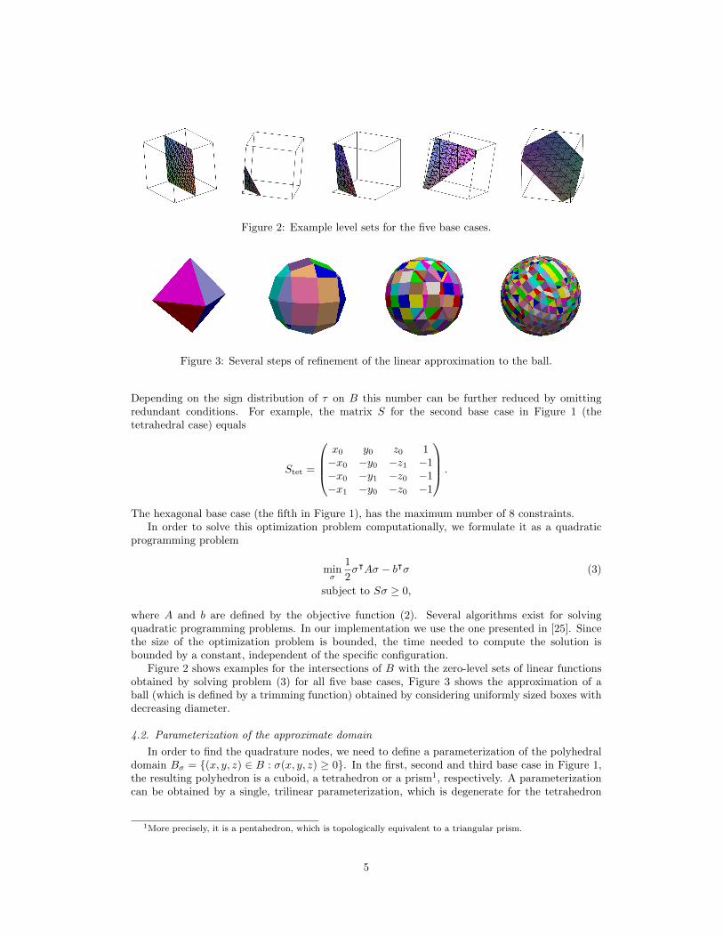
Figure 2: Example level sets for the five base cases.
Figure 3: Several steps of refinement of the linear approximation to the ball.
Depending on the sign distribution of τ on B this number can be further reduced by omittingredundant conditions. For example, the matrix S for the second base case in Figure 1 (thetetrahedral case) equals
Stet =
x0 y0 z0 1−x0 −y0 −z1 −1−x0 −y1 −z0 −1−x1 −y0 −z0 −1
.
The hexagonal base case (the fifth in Figure 1), has the maximum number of 8 constraints.In order to solve this optimization problem computationally, we formulate it as a quadratic
programming problem
minσ
1
2σᵀAσ − bᵀσ (3)
subject to Sσ ≥ 0,
where A and b are defined by the objective function (2). Several algorithms exist for solvingquadratic programming problems. In our implementation we use the one presented in [25]. Sincethe size of the optimization problem is bounded, the time needed to compute the solution isbounded by a constant, independent of the specific configuration.
Figure 2 shows examples for the intersections of B with the zero-level sets of linear functionsobtained by solving problem (3) for all five base cases, Figure 3 shows the approximation of aball (which is defined by a trimming function) obtained by considering uniformly sized boxes withdecreasing diameter.
4.2. Parameterization of the approximate domain
In order to find the quadrature nodes, we need to define a parameterization of the polyhedraldomain Bσ = (x, y, z) ∈ B : σ(x, y, z) ≥ 0. In the first, second and third base case in Figure 1,the resulting polyhedron is a cuboid, a tetrahedron or a prism1, respectively. A parameterizationcan be obtained by a single, trilinear parameterization, which is degenerate for the tetrahedron
1More precisely, it is a pentahedron, which is topologically equivalent to a triangular prism.
5

Figure 4: Parameterization of the linearized domain: Base cases 2-5 (top row) and the subdivisioninto trilinear patches for cases 4 and 5 (bottom row).
and the prism. For the fourth case, we create a multi-patch parameterization that consists of twodegenerate trilinear patches representing prisms. In the fifth base case, we obtain three trilinearpatches (two prisms and a four-sided pyramid). Instances of base cases 2-5 and the splitting intotrilinear patches for cases 3 and 4 are shown in Figure 4.
If B is an instance of a rotation or a reflection of one of the base cases, the parameterization issimply composed with the respective transformation matrix. Whenever the box is in an invertedbase case, i.e. one of the base cases with all signs flipped, we first compute the integral over theentire box B and then subtract the integral defined by the base case.
4.3. Numerical integration
We use a q × q × q-point Gauss rule for the approximation of the integral
Iσf =
∫
Bσ
f(x, y, z) dz dy dx. (4)
This will be denoted as Linearized Trimmed (LT) quadrature rule.If B is an instance of a base case without sign inversion, we obtain
LT[B, τ ]f =
#patches∑
i=1
q3∑
j=1
wijf(xij , yij , z
ij)
︸ ︷︷ ︸(?)
, (5)
where the nodes (xij , yij , z
ij) are the images of the tensor-product Gauss nodes (ξj , ηj , ζj) for the
corresponding patch Gi of the parameterization of Bσ and
wij = wGaussj |det∇Gi(ξj , ηj , ζj)|
6

σ > 0
σ < 0
τ00 < 0 τ10 < 0
τ11 < 0τ01 > 0
σ > 0
σ < 0
τ00 < 0 τ10 < 0
τ11 < 0τ01 > 0
Figure 5: Two-dimensional visualization of the continuity of F . For the approximation on theleft-hand-side, the function F (u) is smooth. For the approximation on the right-hand-side, itis only C0-smooth, because the boundary of the integration domain Bηu crosses the north-eastcorner.
with the tensor-product Gauss weights wGaussj . Otherwise, if B is an inversion of an instance of
a base case (i.e. the signs of τ at the cell vertices are flipped), then the signs of the weights wijare flipped and the sum (?) that corresponds to the trilinear parameterization of the entire box isadded to (5).
5. Corrected linearized trimmed quadrature
In the final step of our method, we add an error correction term to the cell-wise LT quadraturerule in order to alleviate the error caused by the linear approximation of the integration domain.
5.1. The first order correction term
First, we define the linear interpolant between σ and τ for u ∈ [0, 1]:
ηu(x, y, z) = σ(x, y, z) + u(σ(x, y, z)− τ(x, y, z)). (6)
We then consider the integral over the intermediate integration domains
Bηu = (x, y, z) ∈ B : ηu(x, y, z) > 0
as a function of a parameter u ∈ [0, 1], i.e.
F (u) =
∫
Bηu
f(x, y, z) dz dy dx.
Since σ and τ share the sign distribution at the box’ vertices, this function is expected to beC2-smooth for u ∈ [0, 1]. More precisely, it is C2-smooth if the level sets of ηu intersect theboundary of the box transversally and do not cross any vertex or edge as u varies from 0 to 1. Atwo-dimensional illustration of this is shown in Figure 5.
By construction, F (0) = Iσf and F (1) = Iτf . In order to approximate F (1), we perform aTaylor expansion of the function F around u = 0 and evaluate it at u = 1:
F (1) ≈ F (0) + F ′(0). (7)
We call F ′(0) the first order error correction term. The right-hand side, where we use Gaus-sian quadrature to evaluate both contributions, defines the Corrected Linearized Trimmed (CLT)quadrature rule.
7

5.2. Evaluation of the correction term
The first order error correction term admits a simple analytic representation.
Lemma 1. The first order error correction term is equal to
F ′(0) = −∫
σ=0∩Bf
τ
‖∇σ‖ ds. (8)
Proof. We evaluate the derivative of the integral F (u) with respect to the parameter u with thehelp of Reynold’s transport theorem and obtain
F ′(u) =
∫
ηu=0∩Bfvu ds,
where the normal velocity vu is given by
vu = −dduηu
‖∇ηu‖.
From the definition (6) of ηu we infer
∂ηu∂u
= τ − σ
and
∇ηu = ∇σ + u(∇τ −∇σ).
Setting u = 0 and using that σ vanishes on the zero-level we arrive at the representation (8).
For the numerical evaluation of the bivariate integral (8), we consider the subdivision of theintegration domain σ = 0 ∩B, which is defined by the patches covering the polyhedral domainBσ, see Section 4.2. This subdivision consists of at most two triangular and quadrilateral facets,which admit bilinear parameterizations. We use a q × q point Gauss rule to evaluate the con-tributions of the facets to the overall integral. Consequently, the CLT quadrature rule takes theform
CLT[B, τ ]f = LT[B, τ ]f +
#surface patches∑
i=1
q2∑
j=1
vijf(xij , yij , z
ij),
where (xij , yij , z
ij) are the Gauss nodes mapped to the i-th planar patch using the parameterization
Hi and
vij =vGaussj τ(xij , y
ij , z
ij)
√det∇HiT (ξj , ηj)∇Hi(ξj , ηj)
‖∇σ(xij , yij , z
ij)‖2
(9)
with the (2D) tensor-product Gauss weights vGaussj .
In the experiments we will observe that the optimal number of Gauss nodes in each directionwhen using the first order error correction term is q = 2. This is expected, since otherwise theoverall approximation order is dominated by the linear approximation and the correction term.
Higher order correction terms, which are beyond the scope of the present paper, involve edgeintegrals and point evaluations. Clearly, higher order Gauss rules are needed to achieve higheroverall accuracy.
8

5.3. Computational complexity
Next, we consider the computational complexity of both LT and CLT. We assume that eachevaluation of f and τ takes constant time.
Theorem 1. LT requires O(q3) function evaluations.
Proof. The constrained least squares approximation is performed in constant time and thus thecomplexity for finding the approximations σ in all quadrature cells is O(1). Thus, the complexityis dominated by the trivariate quadrature in (4) which is performed up to three times per element.Since we use a q × q × q-point Gauss rule, the overall complexity is O(q3).
Theorem 2. The computational complexity of CLT is the same as the computational complexityof LT.
Proof. The first order correction term (8) consists of a bivariate integral which is approximatedusing the same amount of Gauss nodes per direction as for the trivariate integral (4). Since thenumber of function evaluations in the computation of the weights (9) is constant in h, the overallcomplexity is governed by the trivariate integral in LT and the complexities are asymptoticallythe same.
The overall effort of the compound quadrature rule (which sums up the contributions of theNh sub-boxes, see Section 3) thus evaluates to O(Nhq
3).
6. Numerical examples
We implemented the method using the open source C++ library G+Smo [26]. For solving thequadratic programming problem (3) we use QuadProg++ [27].
6.1. Convergence of the quadrature
In this section, we analyze the behavior of our method with respect to h-refinement. Thismeans that we first subdivide a given geometry uniformly into boxes of size h and then applydifferent quadrature rules to them.
Ellipsoid example. In our first numerical example we use our method to compute the volume ofthe region enclosed by an ellipsoid given implicitly by
τ(x, y, z) = − (x− 0.5)2
a2− (y − 0.5)2
b2− (z − 0.5)2
c2+ 1.
Its piece-wise linear approximation after five steps of refinement is shown in Figure 6. We comparethe convergence of LT and CLT when using two Gauss nodes per direction in both the trivariateintegral in LT and the bivariate integral in the first order error correction term for CLT. Addi-tionally, we compare the two methods with simply using Gauss quadrature for all cells that liecompletely inside the integration domain. This method will be denoted as the inner cell (IC)method.
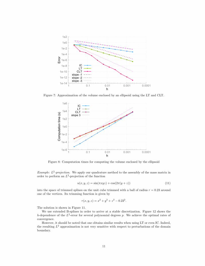
In the plot shown in Figure 7 we observe that the use of error correction increases the orderof convergence by one, resulting in cubic convergence. On the other hand, simply omitting alltrimmed cells gives only linear convergence.
Section 5.3 showed that the computational complexity of both LT and CLT is linear withrespect to the number of quadrature cells. This is the same complexity as for the usual Gaussquadrature over untrimmed cells. Figure 8 shows the computation times needed by our imple-mentation of LT, CLT and IC for various values of the mesh size h. We observe asymptoticallyequivalent computation times of all three methods. The additional computational effort for CLT,which is required for the advanced treatment of the trimmed cells, is more than justified by theincreased accuracy.
9
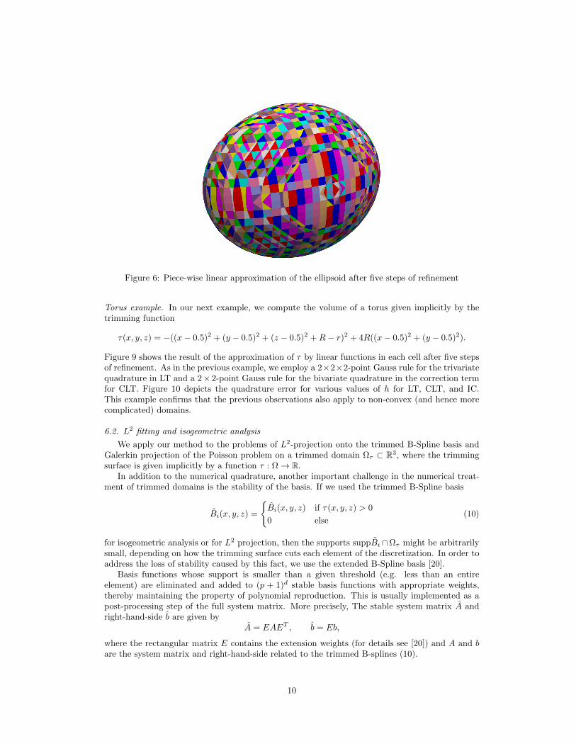
Figure 6: Piece-wise linear approximation of the ellipsoid after five steps of refinement
Torus example. In our next example, we compute the volume of a torus given implicitly by thetrimming function
τ(x, y, z) = −((x− 0.5)2 + (y − 0.5)2 + (z − 0.5)2 +R− r)2 + 4R((x− 0.5)2 + (y − 0.5)2).
Figure 9 shows the result of the approximation of τ by linear functions in each cell after five stepsof refinement. As in the previous example, we employ a 2×2×2-point Gauss rule for the trivariatequadrature in LT and a 2× 2-point Gauss rule for the bivariate quadrature in the correction termfor CLT. Figure 10 depicts the quadrature error for various values of h for LT, CLT, and IC.This example confirms that the previous observations also apply to non-convex (and hence morecomplicated) domains.
6.2. L2 fitting and isogeometric analysis
We apply our method to the problems of L2-projection onto the trimmed B-Spline basis andGalerkin projection of the Poisson problem on a trimmed domain Ωτ ⊂ R3, where the trimmingsurface is given implicitly by a function τ : Ω→ R.
In addition to the numerical quadrature, another important challenge in the numerical treat-ment of trimmed domains is the stability of the basis. If we used the trimmed B-Spline basis
Bi(x, y, z) =
Bi(x, y, z) if τ(x, y, z) > 0
0 else(10)
for isogeometric analysis or for L2 projection, then the supports suppBi ∩Ωτ might be arbitrarilysmall, depending on how the trimming surface cuts each element of the discretization. In order toaddress the loss of stability caused by this fact, we use the extended B-Spline basis [20].
Basis functions whose support is smaller than a given threshold (e.g. less than an entireelement) are eliminated and added to (p + 1)d stable basis functions with appropriate weights,thereby maintaining the property of polynomial reproduction. This is usually implemented as apost-processing step of the full system matrix. More precisely, The stable system matrix A andright-hand-side b are given by
A = EAET , b = Eb,
where the rectangular matrix E contains the extension weights (for details see [20]) and A and bare the system matrix and right-hand-side related to the trimmed B-splines (10).
10
1e-14
1e-12
1e-10
1e-8
1e-6
1e-4
1e-2
1e0
1e2
0.0001 0.001 0.01 0.1 1
Err
or
h
ICLT
CLTslope -1slope -2slope -3
Figure 7: Approximation of the volume enclosed by an ellipsoid using the LT and CLT.
1e-6
1e-4
1e-2
1e0
1e2
1e4
1e6
0.0001 0.001 0.01 0.1 1
Com
puta
tion
time
(s)
h
ICLT
CLTslope 3
Figure 8: Computation times for computing the volume enclosed by the ellipsoid
Example: L2-projection. We apply our quadrature method to the assembly of the mass matrix inorder to perform an L2-projection of the function
u(x, y, z) = sin(πxyz) + cos(2π(y + z)) (11)
into the space of trimmed splines on the unit cube trimmed with a ball of radius r = 0.23 aroundone of the vertices. Its trimming function is given by
τ(x, y, z) = x2 + y2 + z2 − 0.232.
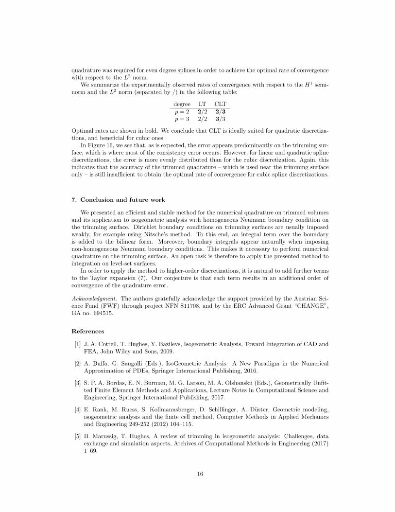
The solution is shown in Figure 11.We use extended B-splines in order to arrive at a stable discretization. Figure 12 shows the
h-dependence of the L2-error for several polynomial degrees p. We achieve the optimal rates ofconvergence.
However, it should be noted that one obtains similar results when using LT or even IC. Indeed,the resulting L2 approximation is not very sensitive with respect to perturbations of the domainboundary.
11

Figure 9: Linear approximation of the torus after some steps of refinement
1e-12
1e-10
1e-8
1e-6
1e-4
1e-2
1e0
1e2
0.0001 0.001 0.01 0.1 1
Err
or
h
Torus
ICLT
CLTslope -1slope -2slope -3
Figure 10: Approximation of the volume of the torus using the LT and CLT.
Example: Poisson equation on cube with spherical cavity. Next, we use our quadrature rules toassemble the stiffness matrix in order to solve the Poisson equation
∆u = f in Ωτ ,∂u∂ν = h on ∂ΩNeumann
τ ,
u = g on ∂ΩDirichletτ
(12)
using Galerkin projection, based on extended B-splines.We use Gauss quadrature with (p+1)3 nodes for the element-wise quadrature on the untrimmed
elements and the linear approximations to the trimmed elements. We also use (p+1)2 Gauss nodesfor the bivariate integral in the error correction term for CLT.
The domain is the unit cube, which has been trimmed by a ball of radius r = 0.23 around thecenter, thus defining the trimming function
τ(x, y, z) = (x− 0.5)2 + (y − 0.5)2 + (z − 0.5)2 − 0.232.
We impose Dirichlet boundary conditions on the boundary of the cube and homogeneous Neumannboundary conditions on the spherical trimming surface. As a manufactured solution fulfilling these
12
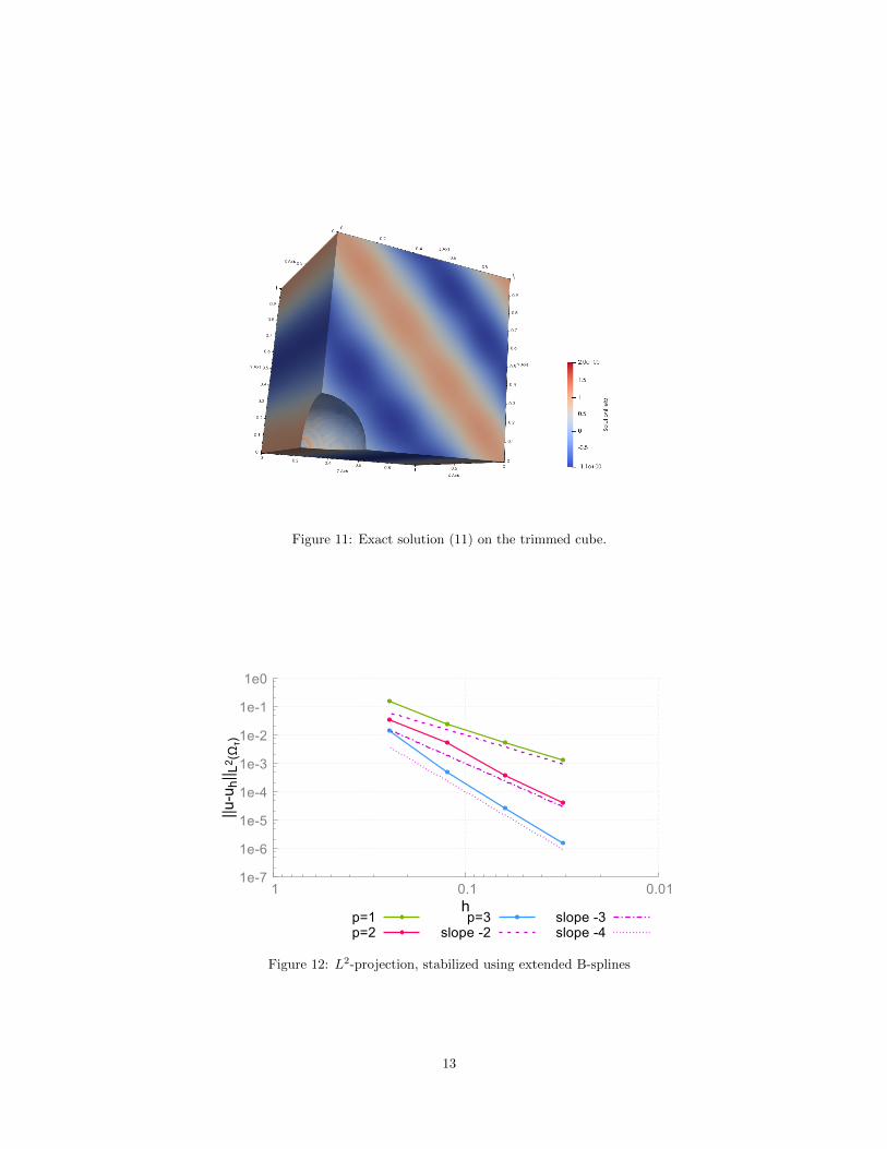
Figure 11: Exact solution (11) on the trimmed cube.
1e-7
1e-6
1e-5
1e-4
1e-3
1e-2
1e-1
1e0
0.01 0.1 1
||u-u
h|| L
2(Ωτ)
hp=1p=2
p=3slope -2
slope -3slope -4
Figure 12: L2-projection, stabilized using extended B-splines
13

Figure 13: The example solution (13) on the trimmed domain clipped with a plane through theorigin (only for the visualization).
boundary conditions we choose
u(x, y, z) =10(x− 1
2 )√(x− 1
2 )2 + (y − 12 )2 + (z − 1
2 )2(13)
+ (τ(x, y, z))2(8 cos(2π(y + z)) + 5 sin(2πxy)).
The first term of u is constant on the lines through the center of the domain, thus fulfillinghomogeneous Neumann boundary conditions on every sphere. The second term as well as itsnormal derivative vanishes on the trimming surface, which is given as the level set τ = 0. Figure 13shows the manufactured solution on the domain Ωτ which was clipped by a plane through its centerfor the visualization.
First we consider the error measured in the H1-seminorm, see Fig. 14, which can be analyzedwith the help of Strang’s lemma [28]. It is bounded by the sum of the approximation error (causedby the discretization) and the consistency error (due to the numerical integration).
For quadratic spline discretizations (p = 2), the approximation error (with respect to theH1-seminorm) converges with order two, and hence it suffices to use a quadrature method thatprovides this level of accuracy. Nevertheless, the CLT provides a small improvement, comparedto LT.
For cubic spline discretizations (p = 3), the approximation error (with respect to the H1-seminorm) converges with order three, and hence one needs to employ quadrature method thatprovides the same accuracy. The plot clearly demonstrates that CLT maintains the overall accu-racy, while LT does not.
Second we consider the error measured in the L2-norm, see Fig. 15. For quadratic splinediscretizations (p = 2), we obtain the full rate of convergence (order 3) when using CLT. However,the use of LT does not provide the full rate, even though it did suffice for optimal (quadratic) H1
seminorm convergence.The situation is different for cubic splines (p = 3): Here, CLT gives only a (sub-optimal)
cubic convergence rate, and an even lower accuracy is obtained when using LT. We conclude thatthe accuracy of the quadrature does not suffice to extend the optimal rate of convergence withrespect to the H1 seminorm (which was guaranteed by Strang’s lemma and demonstrated in Fig.14) to the L2 norm. A similar phenomenon was observed in [29], where a higher accuracy of the
14

1e-4
1e-3
1e-2
1e-1
1e0
1e1
0.01 0.1 1
|u-u
h| H
1(Ωτ)
h
p=2, LTp=2, CLT
p=3, LTp=3, CLT
slope -1slope -2slope -3
Figure 14: h-dependence of the error of the Galerkin approximation in the H1-seminorm.
1e-5
1e-4
1e-3
1e-2
1e-1
1e0
0.01 0.1 1
||u-u
h|| L
2(Ωτ)
h
p=2, LTp=2, CLT
p=3, LTp=3, CLT
slope -2slope -3
Figure 15: h-dependence of the error of the Galerkin approximation in the L2-norm.
15
quadrature was required for even degree splines in order to achieve the optimal rate of convergencewith respect to the L2 norm.
We summarize the experimentally observed rates of convergence with respect to the H1 semi-norm and the L2 norm (separated by /) in the following table:
degree LT CLTp = 2 2/2 2/3p = 3 2/2 3/3
Optimal rates are shown in bold. We conclude that CLT is ideally suited for quadratic discretiza-tions, and beneficial for cubic ones.
In Figure 16, we see that, as is expected, the error appears predominantly on the trimming sur-face, which is where most of the consistency error occurs. However, for linear and quadratic splinediscretizations, the error is more evenly distributed than for the cubic discretization. Again, thisindicates that the accuracy of the trimmed quadrature – which is used near the trimming surfaceonly – is still insufficient to obtain the optimal rate of convergence for cubic spline discretizations.
7. Conclusion and future work
We presented an efficient and stable method for the numerical quadrature on trimmed volumesand its application to isogeometric analysis with homogeneous Neumann boundary condition onthe trimming surface. Dirichlet boundary conditions on trimming surfaces are usually imposedweakly, for example using Nitsche’s method. To this end, an integral term over the boundaryis added to the bilinear form. Moreover, boundary integrals appear naturally when imposingnon-homogeneous Neumann boundary conditions. This makes it necessary to perform numericalquadrature on the trimming surface. An open task is therefore to apply the presented method tointegration on level-set surfaces.
In order to apply the method to higher-order discretizations, it is natural to add further termsto the Taylor expansion (7). Our conjecture is that each term results in an additional order ofconvergence of the quadrature error.
Acknowledgment. The authors gratefully acknowledge the support provided by the Austrian Sci-ence Fund (FWF) through project NFN S11708, and by the ERC Advanced Grant “CHANGE”,GA no. 694515.
References
[1] J. A. Cotrell, T. Hughes, Y. Bazilevs, Isogeometric Analysis, Toward Integration of CAD andFEA, John Wiley and Sons, 2009.
[2] A. Buffa, G. Sangalli (Eds.), IsoGeometric Analysis: A New Paradigm in the NumericalApproximation of PDEs, Springer International Publishing, 2016.
[3] S. P. A. Bordas, E. N. Burman, M. G. Larson, M. A. Olshanskii (Eds.), Geometrically Unfit-ted Finite Element Methods and Applications, Lecture Notes in Computational Science andEngineering, Springer International Publishing, 2017.
[4] E. Rank, M. Ruess, S. Kollmannsberger, D. Schillinger, A. Duster, Geometric modeling,isogeometric analysis and the finite cell method, Computer Methods in Applied Mechanicsand Engineering 249-252 (2012) 104–115.
[5] B. Marussig, T. Hughes, A review of trimming in isogeometric analysis: Challenges, dataexchange and simulation aspects, Archives of Computational Methods in Engineering (2017)1–69.
16

Figure 16: The absolute error |u(x, y, z)−uh(x, y, z)| for p = 1 (top), p = 2 (left) and p = 3 (right)after five steps of refinement using CLT for the assembly. Note that the scales are different!
[6] P. Antolin, A. Buffa, M. Martinelli, Isogeometric Analysis on V-reps: first results (2019).arXiv:1903.03362.
[7] C.-K. Im, S.-K. Youn, The generation of 3d trimmed elements for nurbs-based isogeometricanalysis, International Journal of Computational Methods 15 (7).
[8] S. Xia, X. Qian, Isogeometric analysis with Bezier tetrahedra, Computer Methods in AppliedMechanics and Engineering 316 (2017) 782 – 816.
[9] F. Massarwi, P. Antolin, G. Elber, Volumetric untrimming: Precise decomposition of trimmedtrivariates into tensor products, Computer Aided Geometric Design 71 (2019) 1 – 15.
17

[10] N. Patrikalakis, T. Maekawa, Shape interrogation for computer aided design and manufac-turing, 2010.
[11] C.-Y. Hu, T. Maekawa, N. Patrikalakis, X. Ye, Robust interval algorithm for surface inter-sections, CAD Computer Aided Design 29 (9) (1997) 617–627.
[12] L. Kudela, N. Zander, S. Kollmannsberger, E. Rank, Smart octrees: Accurately integratingdiscontinuous functions in 3d, Computer Methods in Applied Mechanics and Engineering 306(2016) 406 – 426.
[13] A. Nagy, D. Benson, On the numerical integration of trimmed isogeometric elements, Com-puter Methods in Applied Mechanics and Engineering 284 (2015) 165–185.
[14] H. Zhang, R. Mo, N. Wan, An IGA discontinuous Galerkin method on the union of overlappedpatches, Computer Methods in Applied Mechanics and Engineering 326 (2017) 446–480.
[15] S. Kargaran, B. Juttler, S. K. Kleiss, A. Mantzaflaris, T. Takacs, Overlapping multi-patchstructures in isogeometric analysis, NFN Technical Report 82 (2019) 1–34.
[16] M. Bercovier, I. Soloveichik, Overlapping non matching meshes domain decomposition methodin isogeometric analysis (2015). arXiv:1502.03756.
[17] F. Scholz, A. Mantzaflaris, B. Juttler, First order error correction for trimmed quadraturein isogeometric analysis, in: Advanced Finite Element Methods with Applications, LectureNotes in Computational Science and Engineering, Springer International Publishing, 2019, toappear, also available at http://www.gs.jku.at as NFN Report no. 84.
[18] D. A. Cox, T. W. Sederberg, F. Chen, The moving line ideal basis of planar rational curves,Computer Aided Geometric Design 15 (8) (1998) 803 – 827.
[19] G. Taubin, Estimation of planar curves, surfaces, and nonplanar space curves defined by im-plicit equations with applications to edge and range image segmentation, IEEE Transactionson Pattern Analysis and Machine Intelligence 13 (11) (1991) 1115–1138.
[20] K. Hollig, U. Reif, J. Wipper, Weighted extended B-spline approximation of Dirichlet prob-lems, SIAM Journal on Numerical Analysis 39 (2) (2001) 442–462.
[21] B. Marussig, J. Zechner, G. Beer, T. Fries, Stable isogeometric analysis of trimmed geometries,Computer Methods in Applied Mechanics and Engineering 316 (2017) 497–521.
[22] R. Sanches, P. Bornemann, F. Cirak, Immersed b-spline (i-spline) finite element method forgeometrically complex domains, Computer Methods in Applied Mechanics and Engineering200 (13) (2011) 1432 – 1445.
[23] E. Burman, Ghost penalty, Comptes Rendus Mathematique 348 (21) (2010) 1217 – 1220.
[24] D. Elfverson, M. G. Larson, K. Larsson, CutIGA with basis function removal, AdvancedModeling and Simulation in Engineering Sciences 5 (1) (2018) 6.
[25] D. Goldfarb, A. Idnani, A numerically stable dual method for solving strictly convex quadraticprograms, Mathematical Programming 27 (1983) 1–33.
[26] A. Mantzaflaris, F. Scholz, others (see website), G+Smo (Geometry plus Simulation modules)v0.8.1, http://gs.jku.at/gismo (2019).
[27] L. Di Gaspero, Quadprog++, https://github.com/liuq/QuadProgpp.
[28] G. Strang, Approximation in the finite element method, Numerische Mathematik 19 (1972)81–98.
[29] A. Mantzaflaris, B. Juttler, Integration by interpolation and look-up for Galerkin-based iso-geometric analysis, Computer Methods in Applied Mechanics and Engineering 284 (2015)373–400.
18


