Numerical Integration over unit sphere{by using...

Numerical Integration over unit sphere–by using spherical t-designs

Numerical Integration over unit

sphere–by using spherical t-designs

Congpei An1

1,Institute of Computational Sciences, Department of Mathematics,

Jinan University

Spherical Design and Numerical Analysis 2015, SJTU

2015 c 4 � 23 F


Outline

1 Well conditioned spherical designs

2 Numerical verification methods

3 Numerical results of verification methods

4 Numerical integration over unit sphere

5 Performance of Numerical Integrations


Notations

XN = {x1, . . . , xN} ⊂ S2 ={x, y, z ∈ R3 |x2 + y2 + z2 = 1

}Pt = { spherical polynomials of degree ≤ t}

= {polynomials in x, y, z of degree ≤ t restricted to S2}

N = Number of points

t = Degree of polynomials


Spherical coordinates

x1 =

0

0

1

, x2 =

sin(θ2)

0

cos(θ2)

, xi =

sin(θi) cos(φi)

sin(θi) sin(φi)

cos(θi)

, i = 3, . . . , N.

(1)


Background on spherical t−designs

Part I

Background on spherical

t−designs



Definition of Spherical t−design

Definition (Spherical t−design)

The set XN = {x1, . . . ,xN} ⊂ S2 is a spherical t-design if

1

N

N∑j=1

p (xj) =1

4π

∫S2p(x)dω(x) ∀p ∈ Pt, (2)

where dω(x) denotes surface measure on S2.

The definition of spherical t−design was given by Delsarte, Goethals,

Seidel in 1977 [10].



Real Spherical harmonics

Real Spherical harmonics[14]

Y`k : k = 1, . . . , 2` + 1, ` = 0, 1, . . . , tBasis

Pt=Span{Y`k : k = 1, . . . , 2`+ 1, ` = 0, 1, . . . , t}

Orthonormality with respect to L2 inner product

(p, q)L2 =

∫S2p(x)q(x)dω(x),

Normalization Y0,1 = 1√4π

dimPt = (t+ 1)2

Addition Theorem2`+1∑k=1

Y`,k(x)Y`,k(y) =2`+14π P` (x · y) , x, y ∈ S2



Spherical harmonic basis matrix

For t ≥ 1, and N ≥ dim(Pt) = (t+ 1)2, let Y0t be the ((t+ 1)2 − 1) by

N matrix defined by

Y0t (XN ) := [Y`,k(xj)], k = 1, . . . , 2`+ 1, ` = 1, . . . , t; j = 1, . . . , N, (3)

Yt(XN ) :=

[1√4π

eT

Y0t (XN )

]∈ R(t+1)2×N , (4)

where e = [1, . . . , 1]T ∈ RN .

Gt (XN ) := Yt (XN )T Yt (XN ) ∈ RN×N ,

Ht (XN ) := Yt (XN )Yt (XN )T ∈ R(t+1)2×(t+1)2 .



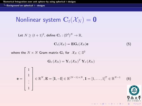
Nonlinear system Ct(XN) = 0

Let N ≥ (t+ 1)2, define Ct : (Sd)N → R,

Ct(XN ) = EGt(XN )e (5)

where the N ×N Gram matrix Gt for XN ⊂ S2

Gt (XN ) = Yt (XN )T Yt (XN )

e =

1

1...

1

∈ RN ,E = [1,−I] ∈ R(N−1)×N , 1 = [1, . . . , 1]T ∈ RN−1 (6)



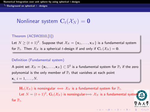
Nonlinear system Ct(XN) = 0

Theorem (ACSW2010,[1])

Let N ≥ (t+ 1)2. Suppose that XN = {x1, . . . ,xN} is a fundamental system

for Pt. Then XN is a spherical t-design if and only if Ct (XN ) = 0.

Definition (Fundamental system)

A point set XN = {x1, . . . , xN} ⊂ S2 is a fundamental system for Pt if the zero

polynomial is the only member of Pt that vanishes at each point

xi, i = 1, . . . , N.

Ht(XN ) is nonsingular ⇐⇒ XN is a fundamental system for Pt.Let N = (t+ 1)2, Gt(XN ) is nonsingular⇐⇒ XN is a fundamental system

for Pt.


Well conditioned spherical designs

II




Definition

Chen and Womersley [8], Chen, Frommer and Lang [9] verified that a

spherical t-design exists in a neighborhood of an extremal system. This leads to

the idea of extremal spherical t-designs, which first appeared in [8] in

N = (t+ 1)2. We here extend the definition to N ≥ (t+ 1)2.

Definition (Extremal spherical designs[1])

A set XN = {x1, . . . ,xN} ⊂ S2 of N ≥ (t+ 1)2 points is a extremal spherical

t-design if the determinant of the matrix

Ht(XN ) := Yt(XN )Yt(XN )T ∈ R(t+1)2×(t+1)2 is maximal subject to the

constraint that XN is a spherical t-design.



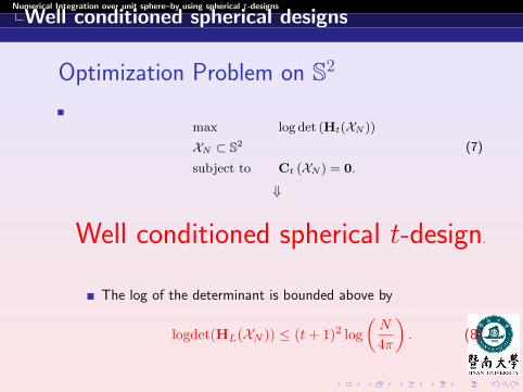
Optimization Problem on S2

max log det (Ht(XN ))

XN ⊂ S2

subject to Ct (XN ) = 0.

(7)

⇓

Well conditioned spherical t-design.

The log of the determinant is bounded above by

logdet(HL(XN )) ≤ (t+ 1)2 log

(N

4π

). (8)


Numerical Verification method

III




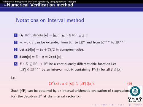
Notations on Interval method

1 By IRn, denote [a] = [a, a], a, a ∈ Rn, a ≤ a

2 +,−, ∗, / can be extended from Rn to IRn and from Rn×n to IRn×n.

3 Let mid[a] = (a+ a)/2 in componentwise.

4 diam[a] = a− a = 2rad [a] ,

5 F : D ⊆ Rn → Rn be a continuously differentiable function.Let

[dF] ∈ IRn×n be an interval matrix containing F′(ξ) for all ξ ∈ [x],

i.e.

{F′(x) : x ∈ [x]} ⊆ [dF] ([x]). (9)

Such [dF] can be obtained by an interval arithmetic evaluation of (expressions

for) the Jacobian F′ at the interval vector [x].



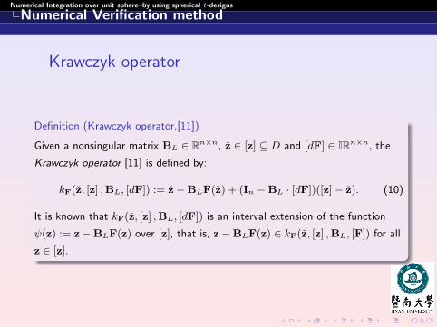
Krawczyk operator

Definition (Krawczyk operator,[11])

Given a nonsingular matrix BL ∈ Rn×n, z ∈ [z] ⊆ D and [dF] ∈ IRn×n, the

Krawczyk operator [11] is defined by:

kF(z, [z] ,BL, [dF]) := z−BLF(z) + (In −BL · [dF])([z]− z). (10)

It is known that kF(z, [z] ,BL, [dF]) is an interval extension of the function

ψ(z) := z−BLF(z) over [z], that is, z−BLF(z) ∈ kF(z, [z] ,BL, [F]) for all

z ∈ [z].



Verification Theorem

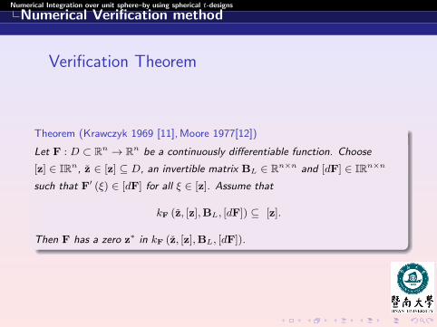
Theorem (Krawczyk 1969 [11], Moore 1977[12])

Let F : D ⊂ Rn → Rn be a continuously differentiable function. Choose

[z] ∈ IRn, z ∈ [z] ⊆ D, an invertible matrix BL ∈ Rn×n and [dF] ∈ IRn×n

such that F′ (ξ) ∈ [dF] for all ξ ∈ [z]. Assume that

kF (z, [z],BL, [dF]) ⊆ [z].

Then F has a zero z∗ in kF (z, [z],BL, [dF]).



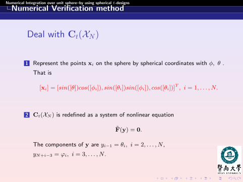
Deal with Ct(XN)

1 Represent the points xi on the sphere by spherical coordinates with φ, θ .

That is

[xi] = [sin([θ])cos([φi]), sin([θi])sin([φi]), cos([θi])]T , i = 1, . . . , N.

2 Ct(XN ) is redefined as a system of nonlinear equation

F(y) = 0.

The components of y are yi−1 = θi, i = 2, . . . , N ,

yN+i−3 = ϕi, i = 3, . . . , N .



1 Use a QR-factorization method at each step to determine the N − 2 least

important components of y, which we label collectively by yN , then write

y := (z,yN ), and define a new function F(z) = F(z,yN ), where

F : RN−1 → RN−1.

2 Using the Krawczyk operator with BL = (mid[dF])−1 we can verify the

existence of a fixed point of z−BLF(z), which is a solution of F(z) = 0.



The estimate on determinant

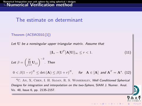
Theorem (ACSW2010,[1])

Let U be a nonsingular upper triangular matrix. Assume that

‖In −UT [A]U‖∞ ≤ r < 1. (11)

Let β =

(N

Πj=1

Ujj

)−2

. Then

0 < β(1− r)N ≤ det (A) ≤ β(1 + r)N , for A ∈ [A] and AT = Aa. (12)

aC. An, X, Chen, I. H. Sloan, R. S. Womersley, Well Conditioned Spherical

Designs for integration and interpolation on the two-Sphere, SIAM J. Numer. Anal.

Vo. 48, Issue 6, pp. 2135-2157.



Proof. We consider a symmetric matrix A ∈ [A]. Noting that UTAU

preserves the symmetric structure, we denote its (real) eigenvalues by

λi(UTAU). Since

max1≤i≤N

| 1− λi(UTAU) |= ρ(In −UTAU

)≤ ‖In −UTAU‖∞ ≤ r,

where ρ is the spectral radius, we have

0 < 1− r ≤ λi(UTAU) ≤ 1 + r, i = 1, . . . , N.

Hence,

(1− r)N ≤ det(UTAU

)≤ (1 + r)N .

Noting that det (U) det(UT)

=

(N

Πj=1

Ujj

)2

= β−1, from

0 < (1− r)N ≤ β−1 det (A) ≤ (1 + r)N ,

we obtain (12). 2



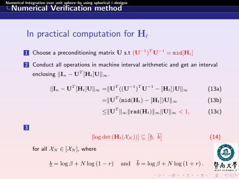
In practical computation for Ht

1 Choose a preconditioning matrix U s.t (U−1)TU−1 = mid[Ht]

2 Conduct all operations in machine interval arithmetic and get an interval

enclosing ‖In −UT [Ht]U‖∞.

‖In −UT [Ht]U‖∞ =‖UT ((U−1)TU−1 − [Ht])U‖∞ (13a)

=‖UT (mid(Ht)− [Ht])U‖∞ (13b)

≤‖UT ‖∞‖rad(Ht)‖∞‖U‖∞ < 1, (13c)

3

[log det (Ht(XN ))] ⊆[b, b

](14)

for all XN ∈ [XN ], where

b = log β +N log (1− r) and b = log β +N log (1 + r) .


Numerical results of verification method

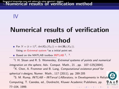
IV

Numerical results of verification

methodFor N = (t+ 1)2, det(Gt(XN )) = det(Ht(XN )).

Using an Extremal system 1as a initial point set.

Based on the MATLAB toolbox INTLAB 2§3.

1I. H. Sloan and R. S. Womersley, Extremal systems of points and numerical

integration on the sphere, Adv. Comput. Math., 21 , pp. 107–125(2004).2X. Chen, A. Frommer and B. Lang, Computational existence proof for

spherical t-designs, Numer. Math., 117 (2011), pp. 289-2053S. M. Rump, INTLAB – INTerval LABoratory, in Developments in Reliable

Computing, T. Csendes, ed., Dordrecht, Kluwer Academic Publishers, pp.

77–104, 1999.



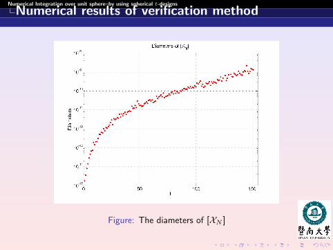
For t = 1, . . . , 151 with N = (t+ 1)2

1 max diam([XN ]) represents the maximum diameter of all computed

enclosures for the parametrization of the respective spherical t-design.

2 [log det(Gt(XN ))] is over 104 for the largest t.



Figure: The diameters of [XN ]



Figure: Middle point values and diameters of [log det(Gt(XN ))]



GeometrySeparation distance–well separated spherical t-design

δXN := minxi,xj∈XN ,i 6=j

dist (xi,xj) ≥π

2t≥ π

2√N.

Figure: The separation of XN with N = (t+ 1)2



Existence of well separated spherical t-designs

For each even N ≥ Cdtd, there exists of a well separated

spherical t-design in the sphere Sd consisting of N points,where Cd is a constant depending only on d4.

4Bondarenko. A., Radchenko, D. Viazovska, M, Well-Separated Spherical

Designs,Constructive Approximation February 2015, Volume 41, Issue 1, pp

93-112



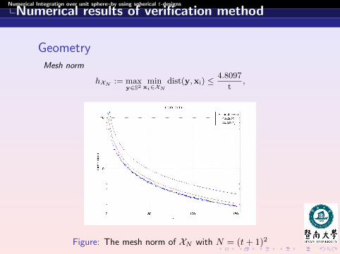
GeometryMesh norm

hXN := maxy∈S2

minxi∈XN

dist(y,xi) ≤4.8097

t,

Figure: The mesh norm of XN with N = (t+ 1)2



GeometryMesh ratio ρXN :=

2hXNδXN

≥ 1

Figure: The mesh ratio of extremal spherical t-designs with N = (t+ 1)2



Conjecture on S2

Let Cδ, Ch be constants. A lower bound on the separation of well

conditioned spherical t-designs for

δXN ≥ CδN− 1

2 ,

combined with the known upper bounds on mesh norm

hXN ≤ ChN12

would give the uniform bound

ρXN ≤2ChCδ

independent of t, N. (15)



An example

Figure: Well conditioned 49 design with 2500 points



A question

Can we verify Womersley’s efficient sphericalt-designs successfully by using Interval analysis?


Numerical Integrations over unit sphere

V


1 Bivariate trapezoidal rule5, with q = 2.5.

2 Well conditioned spherical t-designs

3 Equal area points6

5K. Atkinson. Quadrature of singular integrands over surfaces. Electron.

Trans. Numer. Anal., 7:133–150, 2004.6EA. Rakhmanov, EB. Saff, and Y. Zhou, Minimimal discrete energy on the

sphere. Math. Res. Lett., 11(6): 647–662, 1994



Bivariate trapezoidal rule

For the problem of approximate

I(f) =

∫S2f(x)dω(x)

in which f is several times continuously differentiable over the

unit sphere S2, we can use spherical coordinates to rewrite it as

I(f) =

∫ π

0

∫ 2π

0

f(cosφ sin θ, sinφ sin θ, cos θ) sin θdφdθ

.



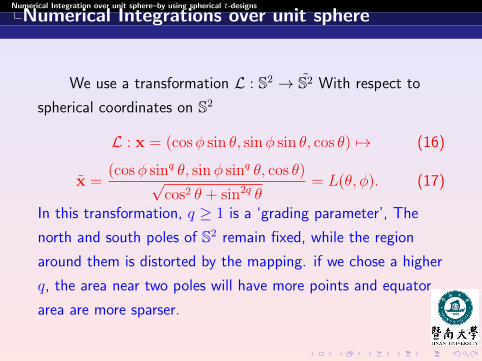
We use a transformation L : S2 → S2 With respect to

spherical coordinates on S2

L : x = (cosφ sin θ, sinφ sin θ, cos θ) 7→ (16)

x =(cosφ sinq θ, sinφ sinq θ, cos θ)√

cos2 θ + sin2q θ= L(θ, φ). (17)

In this transformation, q ≥ 1 is a ‘grading parameter’, The

north and south poles of S2 remain fixed, while the region

around them is distorted by the mapping. if we chose a higher

q, the area near two poles will have more points and equator

area are more sparser.



The integral I(f) becomes

I(f) =

∫S2f(Lx)JL(x)dω(x)

with JL(x) the jacobian of the mapping L,

JL(x) = |DφL(θ, φ)×DθL(θ, φ)| =sin2q−1 θ(q cos2 θ + sin2 θ)

(cos2θ + sin2q θ)32

.

In spherical coordinates,

I(f) =

∫ π

0

sin2q−1 θ(q cos2 θ + sin2 θ)


∫ 2π

0

f(ξ, η, ζ)dφdθ,

(ξ, η, ζ) =(cosφ sinq θ, sinφ sinq θ, cos θ)√

cos2 θ + sin2q θ(18)



For n ≥ 1, let h = π/n, and

φj = θj = jh∫ π

0

∫ 2π

0

g(sin θ, cos θ, sinφ, cosφ) dφ dθ

≈ h2n−1∑k=1

2n∑j=1

g(sin θk, cos θk, sinφj, cosφj) ≡ In,

g =sin2q−1 θ(q cos2 θ + sin2 θ)


f(ξ, η, ζ).

Error satisfies

I − In = O(hk) f ∈ Ck(S2)



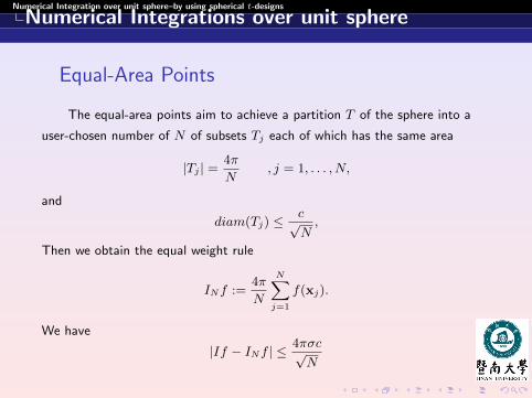
Equal-Area Points

The equal-area points aim to achieve a partition T of the sphere into a

user-chosen number of N of subsets Tj each of which has the same area

|Tj | =4π

N, j = 1, . . . , N,

and

diam(Tj) ≤c√N,

Then we obtain the equal weight rule

INf :=4π

N

N∑j=1

f(xj).

We have

|If − INf | ≤4πσc√N



Geometry of different nodes

(a) Bi. trapezoidal rule (b) Equal area points (c) spherical t-design



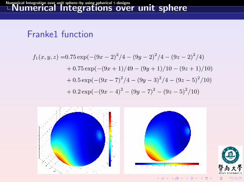
Franke1 function

f1(x, y, z) =0.75 exp(−(9x− 2)2/4− (9y − 2)2/4− (9z − 2)2/4)

+ 0.75 exp(−(9x+ 1)/49− (9y + 1)/10− (9z + 1)/10)

+ 0.5 exp(−(9x− 7)2/4− (9y − 3)2/4− (9z − 5)2/10)

+ 0.2 exp(−(9x− 4)2 − (9y − 7)2 − (9z − 5)2/10)

Figure: f1



C0 function

f2(x) = sin2(1 + ||x||1)/10

is not continuously differentiable at points where any component of x is zero.

Figure: f2



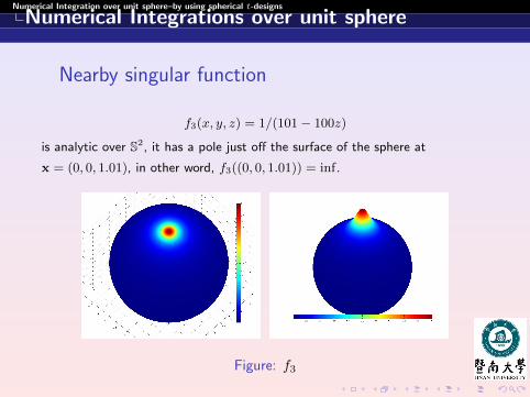
Nearby singular function

f3(x, y, z) = 1/(101− 100z)

is analytic over S2, it has a pole just off the surface of the sphere at

x = (0, 0, 1.01), in other word, f3((0, 0, 1.01)) = inf.

Figure: f3



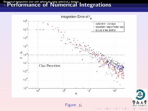
Cap function with R = 13 , center x0 = (0, 0, 1)T .

f4(x) =

cos2(π2

dist(x, x0)/R) if dist(x, x0) < R

0 if dist(x, x0) ≥ R,

Figure: f4


Performance of Numerical Integrations

VI

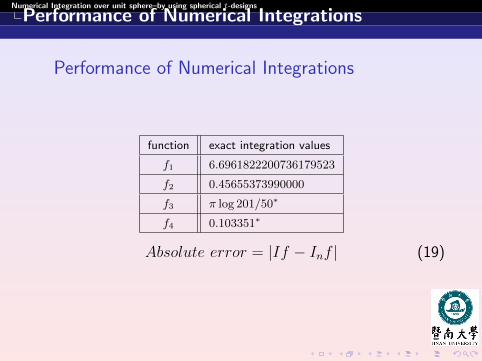
Performance of Numerical

Integrations




function exact integration values

f1 6.6961822200736179523

f2 0.45655373990000

f3 π log 201/50∗

f4 0.103351∗

Absolute error = |If − Inf | (19)



Figure: f1



Figure: f2



Figure: f3



Figure: f4



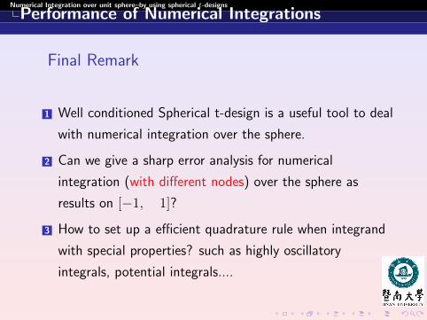
Final Remark

1 Well conditioned Spherical t-design is a useful tool to deal

with numerical integration over the sphere.

2 Can we give a sharp error analysis for numerical

integration (with different nodes) over the sphere as

results on [−1, 1]?

3 How to set up a efficient quadrature rule when integrand

with special properties? such as highly oscillatory

integrals, potential integrals....



Thank you very much!


REFERENCES

REFERENCES


REFERENCES

[1] C. An, X, Chen, I. H. Sloan, R. S. Womersley, Well Conditioned Spherical Designs for integration and

interpolation on the two-Sphere, SIAM J. Numer. Anal. Vo. 48, Issue 6, pp. 2135-2157.

[2] C. An, X, Chen, I. H. Sloan, R. S. Womersley, Regularized least squares approximation on sphere

using spherical designs, SIAM J. Numer. Anal. Vol. 50, No. 3, pp. 1513õ1534.

[3] C.An, Distributing points on the unit sphere and spherical designs, Ph.D Thesis, The Hong Kong

Polytechnic University, 2011.

[4] E. Bannai , R.M. Damerell, Tight spherical designs I. Math Soc Japan 31(1): 199-207,1979.

[5] R. Bauer, Distribution of points on a sphere with application to star catalogs , J. Guidance, Control, and

Dynamics, 23 (2000), pp. 130–137.

[6] A. Bondarenko, D. Radchenko, and M. Viazovska, Optimal asymptotic bounds for spherical designs.

ArXiv:1009.4407v1[math.MG], 2011.

[7] A. Bondarenko, D. Radchenko, and M. Viazovska,Well separated spherical designs. ArXiv:1303.5991

[math.MG],2013.

[8] X. Chen and R. S. Womersley, Existence of solutions to systems of undetermined equations and

spherical designs, SIAM J. Numer. Anal., 44 (2006), pp. 2326–2341.

[9] X. Chen, A. Frommer and B. Lang, Computational existence proof for spherical t-designs, Numer.

Math., 117 (2011), pp. 289-205

[10] P. Delsarte, J. M. Goethals and J. J. Seidel, Spherical codes and designs, Geom. Dedicata, 6

(1977), pp. 363–388.

[11] R. Krawczyk, Newton-Algorithmen zur Bestimmung von Nullstellen mit Fehlerschranken, Computing, 4 ,

pp. 187–201(1969).

[12] R. E. Moore, A test for existence of solutions to nonlinear systems, SIAM J. Numer. Anal., 14 , pp.

611–615(1977).

[13] S. M. Rump, INTLAB – INTerval LABoratory, in Developments in Reliable Computing, T. Csendes, ed.,

Dordrecht, Kluwer Academic Publishers, pp. 77–104, 1999.

[14] C. Muller, Spherical Harmonics, vol. 17 of Lecture Notes in Mathematics, Springer Verlag, Berlin,

New-York, 1966.

[15] R. J. Renka, Multivariate interpolation of large sets of scattered data, ACM Trans. Math. Software, 14

(1988), pp. 139–148.

[16] P.D. Seymour and T. Zaslavsky ,Averaging sets: A generalization of mean values and spherical designs.

Advances in Mathematics, vol. 52, pp. 213-240,1984.

[17] I. H. Sloan, Polynomial interpolation and hyperinterpolation over general regions, J. Approx. Theory, 83

(1995), pp. 238–254.

[18] I. H. Sloan and R. S. Womersley, Extremal systems of points and numerical integration on the sphere,

Adv. Comput. Math., 21 , pp. 107–125(2004).

[19] I. H. Sloan and R. S. Womersley, Constructive polynomial approximation on the sphere, J. Approx.

Theory, 103 (2000), pp. 91-98.

[20] I. H. Sloan and R. S. Womersley, Filtered hyperinterpolation: A constructive polynomial approximation

on the sphere, Int. J. Geomath., 3, pp. 95õ117, 2012.

Date post:	27-Apr-2020
Category:	Documents
Upload:	others
View:	27 times
Download:	0 times

Numerical Integration over unit sphere{by using...

Documents