Page 1
NUMERICAL INVESTIGATION OF THE
FLOW BEHAVIOR INTO THE INLET
GUIDE VANE SYSTEM (IGV)
Publication was supported by project: „Budování excelentního vědeckého týmu pro
experimentální a numerické modelování v mechanice tekutin a termodynamice“
Project registration number: CZ.1.07/2.3.00/20.0139
Ing. Roman GÁŠPÁR
Ph.D. candidate
Univerzitní 22, 306 14, Pilsen
[email protected]
University of West Bohemia » Department of Power System Engineering
Page 2
I
TABLE OF CONTENTS
Table of contents ...................................................................................................................................... I
Figures ................................................................................................................................................... III
Tables .................................................................................................................................................... IV
1 CFD – Computational fluid dynamics............................................................................................. 5
1.1 Mathematical principle of the CFD ......................................................................................... 5
1.2 SOLVING A CFD PROBLEM ............................................................................................... 5
2 Introduction and motivation ............................................................................................................ 7
3 Geometry ......................................................................................................................................... 9
3.1 Solver and Arrangement of the Files ....................................................................................... 9
3.2 File Naming ............................................................................................................................. 9
3.3 Gometry Generator .................................................................................................................. 9
4 Mesh .............................................................................................................................................. 12
4.1 Solver and Arrangement of the Files ..................................................................................... 12
4.2 Mesh Generation ................................................................................................................... 12
5 Boundary Conditions and Calculation .......................................................................................... 14
5.1 Solver and Arrangement of the Files ..................................................................................... 14
5.2 Boundary Conditions and Numerical Solver Settings ........................................................... 14
5.2.1 Fluid models .................................................................................................................. 14
5.2.2 Turbulence model .......................................................................................................... 14
5.2.3 Boundary conditions ..................................................................................................... 15
5.2.4 Boundary conditions applied in this case ...................................................................... 15
6 Results ........................................................................................................................................... 17
6.1 Solver and Arrangement of the Files ..................................................................................... 17
6.2 Investigated Parameters ......................................................................................................... 17
6.3 Tables Description................................................................................................................. 17
6.4 Tables .................................................................................................................................... 19
6.5 Pressure distribution along the wall ...................................................................................... 21
Page 3
II
6.6 Velocity fields ....................................................................................................................... 24
7 Conclusions ................................................................................................................................... 26
7.1 Suggestions for further work ................................................................................................. 26
Page 4
III
FIGURES
Fig. 1 Results of mesh sensibility study ............................................................................................ 7
Fig. 2 Flow separation – Sharp edge (left) – Blended Edge (right) ................................................... 8
Fig. 3 First view to the “GEOMETRY GENERATOR” project ....................................................... 9
Fig. 4 Generated IGV_INLET_VOL (left) and IGV_OUTLET_VOL (right) ................................ 10
Fig. 5 Generated IGV_4BLADE_VOLUME (15 deg.) ................................................................... 10
Fig. 6 Parameters tab. – Setting angle of blades .............................................................................. 10
Fig. 7 IGV assembly generation ...................................................................................................... 11
Fig. 8 IGV’s mesh (green) with extra volume (purple) ................................................................... 13
Fig. 9 Boundary conditions for the IGV channel ............................................................................ 16
Fig. 10 Evaluated areas ...................................................................................................................... 18
Fig. 11 Static pressure distribution along the wall for 4,4 [kg.s-1] .................................................... 21
Fig. 12 Static pressure distribution along the wall for 4,6 [kg.s-1] .................................................... 21
Fig. 13 Static pressure distribution along the wall for 4,8 [kg.s-1] .................................................... 22
Fig. 14 Static pressure distribution along the wall for 5,0 [kg.s-1] .................................................... 22
Fig. 15 Static pressure distribution along the wall for 5,2 [kg.s-1] .................................................... 23
Fig. 16 Static pressure distribution along the wall for 5,4 [kg.s-1] .................................................... 23
Fig. 17 Velocity field – blade position 0°; mass flow 5,0 [kg.s-1] ..................................................... 24
Fig. 18 Velocity field – blade position 20°; mass flow 5,0 [kg.s-1] ................................................... 24
Fig. 19 Velocity field – blade position 40°; mass flow 5,0 [kg.s-1] ................................................... 25
Fig. 20 Velocity field – blade position 60°; mass flow 5,0 [kg.s-1] ................................................... 25
Page 5
IV
TABLES
Tab. 1 Mesh size and Y+ values for different cases ......................................................................... 12
Tab. 2 Pressure drop for different blade positions and mass flow rate (4,4 [kg.s-1] – 4,8 [kg.s-1]) .. 19
Tab. 3 Pressure drop for different blade positions and mass flow rate (5,0 [kg.s-1] – 5,4 [kg.s-1]) . 20
Page 6
NUMERICAL INVESTIGATION OF THE FLOW BEHAVIOR INTO THE INLET GUIDE VANE SYSTEM (IGV)
5
1 CFD – COMPUTATIONAL FLUID DYNAMICS
Computational Fluid Dynamics (CFD) is a method for simulating behavior of the fluid flow or the system
involving heat transfer, radiation, and so on. This method uses computers for solving special equations over
a region of interest with known conditions on the boundaries.
The first mentions about CFD were on around 1910; more interest in CFD began to show after the Second
World War, however, more practical use came up with the expansion of computer technology at the end of
the 80s and early 90s. Since these times CFD has been more or less on a theoretical level.
Nowadays, the CFD in one of the basic design tools helping to reduce the design time and to increase
effectivity of engineering work. CFD is widely used on fields of power and energy, engine industry,
aerodynamics, thermodynamic, aeronautics etc.
1.1 MATHEMATICAL PRINCIPLE OF CFD
It is necessary to solve several equations, which describe processes of momentum, heat end mass transfer
etc., to describe and predict a flow behavior. These equations are known as Navier-Stokes equations. These
equations are defined from the mathematical point of view as partial differential equations. There were
derived in the early nineteenth century. These equations can be discretized and solved numerically.
There are a lot of different methods to solve these equations and there are several codes. The solution
presented here has been achieved by the commercial software ANSYS and its particular parts. The main
solver, which solves equations mentioned above, is called CFX and it’s based on the finite volume
technique.
In case of the finite volume technique the investigated region is divided to small regions (volumes). The
equations mentioned above are discretized and solved iteratively for each of these small volumes.
Nowadays complicated industrial computations include 10, 20 or more than 50 mil. volumes, depending
on the case.
1.2 SOLVING A CFD PROBLEM
From the global point of view there are 5 steps to reach data and solution from CFD simulation:
1) Defining the geometry of region of interest – In this step it is necessary to determine the region of
interest. Modeling big regions or volumes is very time consuming. Before the start it must be clear,
which effects are significant on the investigated volume and which effects are not. It is necessary
to have basic knowledge and vision about the flow behavior before starting the simulation. Based
on this knowledge it determines necessary simplifications. After the volume creation it creates
surface boundary names.
Page 7
NUMERICAL INVESTIGATION OF THE FLOW BEHAVIOR INTO THE INLET GUIDE VANE SYSTEM (IGV)
6
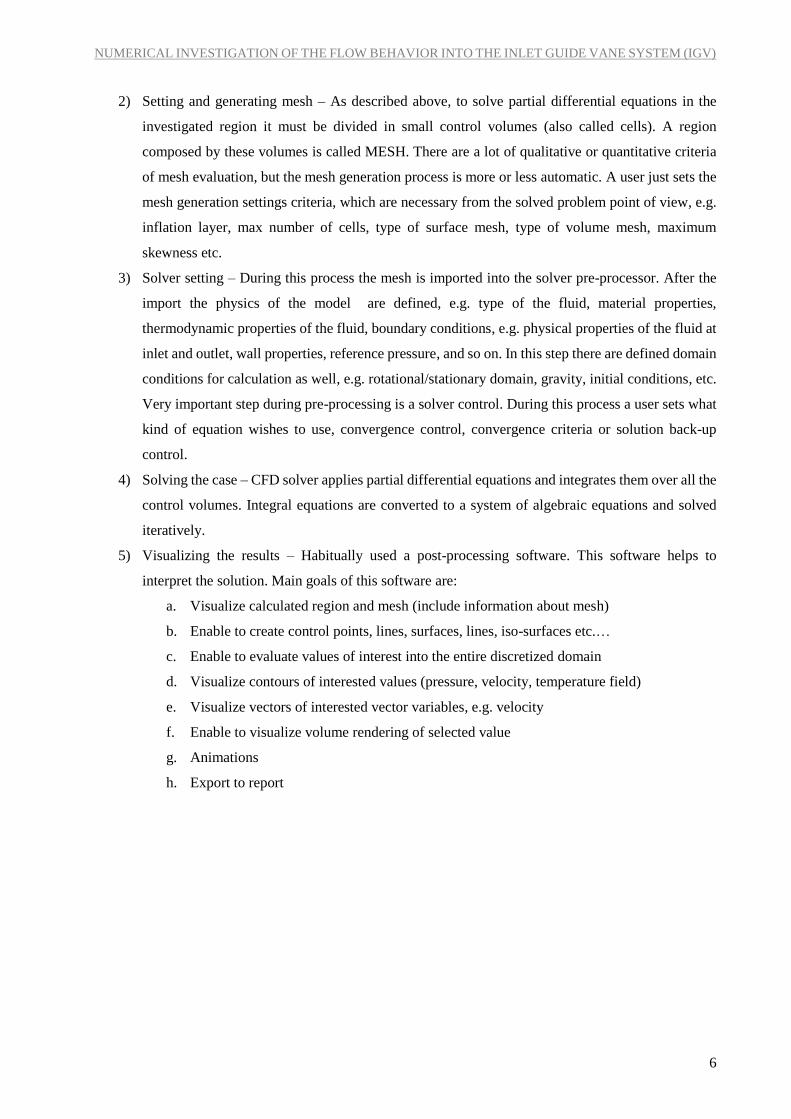
2) Setting and generating mesh – As described above, to solve partial differential equations in the
investigated region it must be divided in small control volumes (also called cells). A region
composed by these volumes is called MESH. There are a lot of qualitative or quantitative criteria
of mesh evaluation, but the mesh generation process is more or less automatic. A user just sets the
mesh generation settings criteria, which are necessary from the solved problem point of view, e.g.
inflation layer, max number of cells, type of surface mesh, type of volume mesh, maximum
skewness etc.
3) Solver setting – During this process the mesh is imported into the solver pre-processor. After the
import the physics of the model are defined, e.g. type of the fluid, material properties,
thermodynamic properties of the fluid, boundary conditions, e.g. physical properties of the fluid at
inlet and outlet, wall properties, reference pressure, and so on. In this step there are defined domain
conditions for calculation as well, e.g. rotational/stationary domain, gravity, initial conditions, etc.
Very important step during pre-processing is a solver control. During this process a user sets what
kind of equation wishes to use, convergence control, convergence criteria or solution back-up
control.
4) Solving the case – CFD solver applies partial differential equations and integrates them over all the
control volumes. Integral equations are converted to a system of algebraic equations and solved
iteratively.
5) Visualizing the results – Habitually used a post-processing software. This software helps to
interpret the solution. Main goals of this software are:
a. Visualize calculated region and mesh (include information about mesh)
b. Enable to create control points, lines, surfaces, lines, iso-surfaces etc.…
c. Enable to evaluate values of interest into the entire discretized domain
d. Visualize contours of interested values (pressure, velocity, temperature field)
e. Visualize vectors of interested vector variables, e.g. velocity
f. Enable to visualize volume rendering of selected value
g. Animations
h. Export to report
Page 8
NUMERICAL INVESTIGATION OF THE FLOW BEHAVIOR INTO THE INLET GUIDE VANE SYSTEM (IGV)
7
2 INTRODUCTION AND MOTIVATION
The hereinafter described CFD investigation is connected with the integrated gas turbine with recycling
process. This facility was supervised by the Chair of Thermal Power Machinery and Plants. Besides this
investigation at that facility there were several other investigations:
Performance of power plant process
Steam injection for high steam mass flow (optimal position, optimum steam parameters, mix with
flue gases)
Impact on flow, cooling, performance and life of the turbine
Affect behavior and performance of the compressor
Water treatment (procedures, operating at elevated temperatures)
The aim of the project was CFD (Computational Fluid Dynamics) investigation of The Inlet Guide Vane
(IGV) System integrated into the gas turbine. The process of the IGV system numerical simulation is
described below step by step. The work started with geometry generation and it follows by generating mesh
and setting up calculation. The last part includes important results and conclusions. It also includes a
description of the position of the important files, which were forwarded to the host institution.
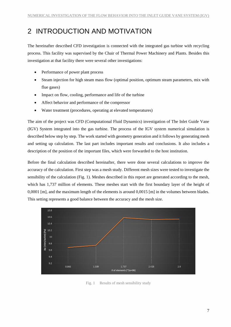
Before the final calculation described hereinafter, there were done several calculations to improve the
accuracy of the calculation. First step was a mesh study. Different mesh sizes were tested to investigate the
sensibility of the calculation (Fig. 1). Meshes described in this report are generated according to the mesh,
which has 1,737 million of elements. These meshes start with the first boundary layer of the height of
0,0001 [m], and the maximum length of the elements is around 0,0015 [m] in the volumes between blades.
This setting represents a good balance between the accuracy and the mesh size.
Fig. 1 Results of mesh sensibility study
Page 9
NUMERICAL INVESTIGATION OF THE FLOW BEHAVIOR INTO THE INLET GUIDE VANE SYSTEM (IGV)
8
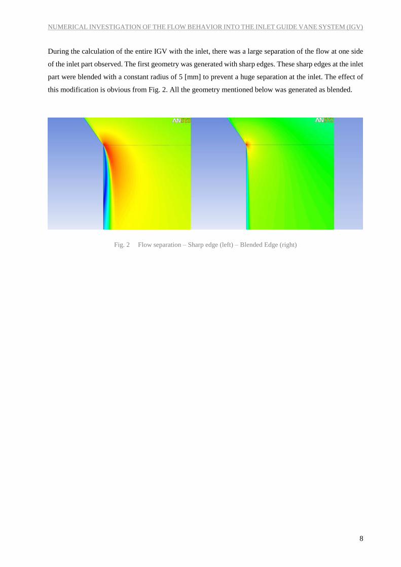
During the calculation of the entire IGV with the inlet, there was a large separation of the flow at one side
of the inlet part observed. The first geometry was generated with sharp edges. These sharp edges at the inlet
part were blended with a constant radius of 5 [mm] to prevent a huge separation at the inlet. The effect of
this modification is obvious from Fig. 2. All the geometry mentioned below was generated as blended.
Fig. 2 Flow separation – Sharp edge (left) – Blended Edge (right)
Page 10
NUMERICAL INVESTIGATION OF THE FLOW BEHAVIOR INTO THE INLET GUIDE VANE SYSTEM (IGV)
9
3 GEOMETRY
3.1 SOLVER AND ARRANGEMENT OF THE FILES
Geometry dimensions were measured at the real IGV system and were implemented into the CAD model.
The IGV CAD model has been generated at the ANSYS Design Modeler ver. 14.0. This software with a
source of files is able to generate the IGV geometry with different angles of the guide vanes. Source files
are located at IGV/GEOMETRY/GEOMETRY_GENERATOR.
3.2 FILE NAMING
IGV_0_NC_B
IGV – indicates that the IGV part was investigated
0 – indicates the angle of the blades
NC – indicates that the computation is without the compressor part (No Compressor)
B/S – indicates that the inlet channel is Blended or Sharp
3.3 GEOMETRY GENERATOR
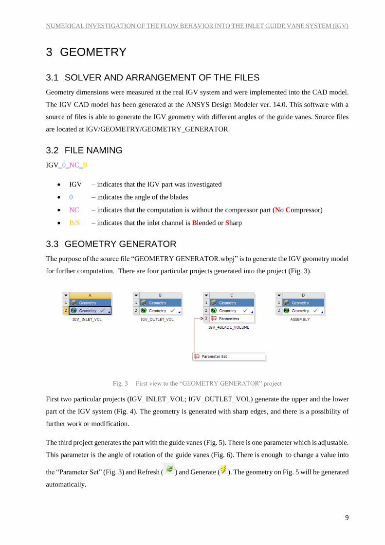
The purpose of the source file “GEOMETRY GENERATOR.wbpj” is to generate the IGV geometry model
for further computation. There are four particular projects generated into the project (Fig. 3).
Fig. 3 First view to the “GEOMETRY GENERATOR” project
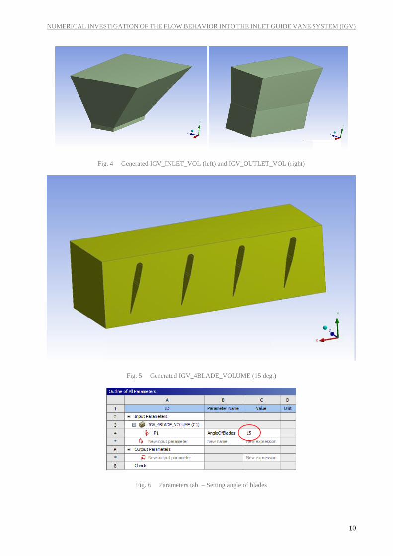
First two particular projects (IGV_INLET_VOL; IGV_OUTLET_VOL) generate the upper and the lower
part of the IGV system (Fig. 4). The geometry is generated with sharp edges, and there is a possibility of
further work or modification.
The third project generates the part with the guide vanes (Fig. 5). There is one parameter which is adjustable.
This parameter is the angle of rotation of the guide vanes (Fig. 6). There is enough to change a value into
the “Parameter Set” (Fig. 3) and Refresh ( ) and Generate ( ). The geometry on Fig. 5 will be generated
automatically.
Page 11
NUMERICAL INVESTIGATION OF THE FLOW BEHAVIOR INTO THE INLET GUIDE VANE SYSTEM (IGV)
10
Fig. 4 Generated IGV_INLET_VOL (left) and IGV_OUTLET_VOL (right)
Fig. 5 Generated IGV_4BLADE_VOLUME (15 deg.)
Fig. 6 Parameters tab. – Setting angle of blades
Page 12
NUMERICAL INVESTIGATION OF THE FLOW BEHAVIOR INTO THE INLET GUIDE VANE SYSTEM (IGV)
11
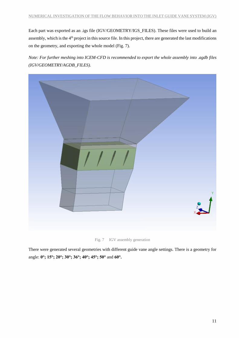
Each part was exported as an .igs file (IGV/GEOMETRY/IGS_FILES). These files were used to build an
assembly, which is the 4th project in this source file. In this project, there are generated the last modifications
on the geometry, and exporting the whole model (Fig. 7).
Note: For further meshing into ICEM-CFD is recommended to export the whole assembly into .agdb files
(IGV/GEOMETRY/AGDB_FILES).
Fig. 7 IGV assembly generation
There were generated several geometries with different guide vane angle settings. There is a geometry for
angle: 0°; 15°; 20°; 30°; 36°; 40°; 45°; 50° and 60°.
Page 13
NUMERICAL INVESTIGATION OF THE FLOW BEHAVIOR INTO THE INLET GUIDE VANE SYSTEM (IGV)
12
4 MESH
4.1 SOLVER AND ARRANGEMENT OF THE FILES
All mesh files for the above mentioned cases can be found in IGV/MESH/IGV_CHANNEL_FILES folder.
Folders contain ICEM-CFD files, which allow reproducing the entire meshing process. CFX5_FILES
folder contains .cfx5 mesh files, which are prepared for the import into CFX-Pre. Meshes were prepared
into ICEM-CFD ver. 14.0.
4.2 MESH GENERATION
Mesh for each case was generated separately (Tab. 1).
All hexahedral with global quality criterion > 0.4
Tab. 1 shows a number of elements for each case and the global maximum of the Y+ value
First layer distance 0.0001 [m]
Growth rate: 1.2
Additional volumes were created
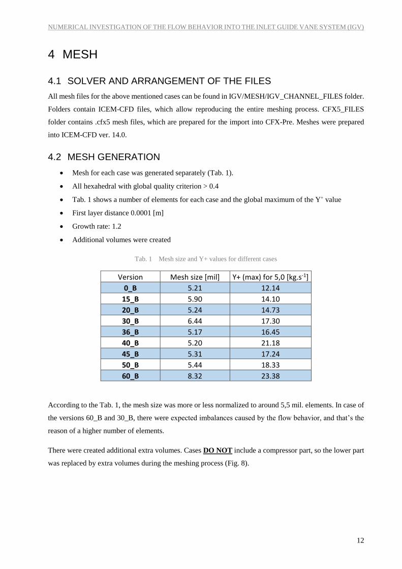
Tab. 1 Mesh size and Y+ values for different cases
Version Mesh size [mil] Y+ (max) for 5,0 [kg.s-1]
0_B 5.21 12.14
15_B 5.90 14.10
20_B 5.24 14.73
30_B 6.44 17.30
36_B 5.17 16.45
40_B 5.20 21.18
45_B 5.31 17.24
50_B 5.44 18.33
60_B 8.32 23.38
According to the Tab. 1, the mesh size was more or less normalized to around 5,5 mil. elements. In case of
the versions 60_B and 30_B, there were expected imbalances caused by the flow behavior, and that’s the
reason of a higher number of elements.
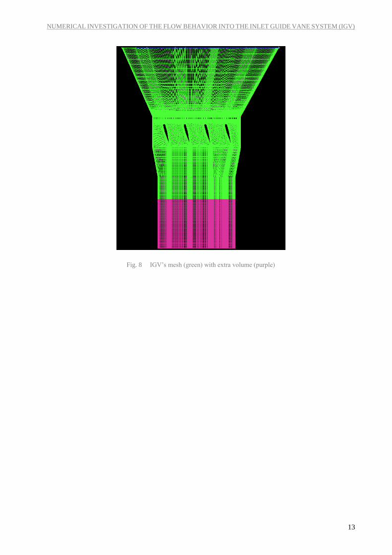
There were created additional extra volumes. Cases DO NOT include a compressor part, so the lower part
was replaced by extra volumes during the meshing process (Fig. 8).
Page 14
NUMERICAL INVESTIGATION OF THE FLOW BEHAVIOR INTO THE INLET GUIDE VANE SYSTEM (IGV)
13
Fig. 8 IGV’s mesh (green) with extra volume (purple)
Page 15
NUMERICAL INVESTIGATION OF THE FLOW BEHAVIOR INTO THE INLET GUIDE VANE SYSTEM (IGV)
14
5 BOUNDARY CONDITIONS AND CALCULATION
5.1 SOLVER AND ARRANGEMENT OF THE FILES
Calculation was provided by ANSYS CFX ver. 14.0. Files for modifying calculations are in
IGV/CALCULATIONS/CFX_FILES folder. Prepared .def files to run calculation are situated into
IGV/CALCULATIONS/DEF_FILES folder. There are another subfolders inside the folders. Numbers
indicate the current mass flow rate of e.g. 5_0, it means 5.0 [kg.s-1].
5.2 BOUNDARY CONDITIONS AND NUMERICAL SOLVER SETTINGS
Steady state calculation with a stationary domain
o Applied a false time step (solver formulation is robust and fully implicit)
Material: Air Ideal Gas
o Properties of this fluid is calculated by the equation of state
𝑝
𝜌= 𝑅. 𝑇
o cp =cp(T)
o dh=cp.dT
5.2.1 Fluid models
Basic fluid can be described by three basic equations:
The continuity equation:
𝜕𝜌
𝜕𝑡+ ∇. (𝜌. 𝑼) = 0
The momentum equation:
𝜕(𝜌. 𝑼)
𝜕𝑡+ ∇. (𝜌. 𝑼 × 𝑼) = −∇𝑝 + ∇𝜏 + 𝑺𝑀
The Total Energy Equation
𝜕(𝜌 ℎ𝑡𝑜𝑡)
𝜕𝑡−
𝜕𝑝
𝜕𝑡+ 𝛻. (𝜌 𝑼 ℎ𝑡𝑜𝑡) = 𝛻. (𝜆 𝛻𝑇) + 𝛻. (𝑼. 𝜏) + 𝑼. 𝑺𝑀 + 𝑺𝐸
5.2.2 Turbulence model
Shear Stress Transport turbulence model with an automatic wall function is very well fitted to modeling a
boundary layer, which was very important in this case, especially because the “WALL” boundary condition
was set to “SMOOTH”. This model gives a highly accurate flow separation prediction and free shear flow
Page 16
NUMERICAL INVESTIGATION OF THE FLOW BEHAVIOR INTO THE INLET GUIDE VANE SYSTEM (IGV)
15
prediction far from the wall as well. This model is based on a k-ω model, and the proper transport
behavior can be obtained by a limiter to the formulation of the eddy-viscosity.
5.2.3 Boundary conditions
After the mesh import, the CFX generates the topology of the calculation domain. The imported mesh is
divided into primitive regions (volumes, surfaces). At the beginning, these regions are defined as a part of
“Default Domain”. In the next steps it is necessary to define what kind of boundaries are these regions.
These boundaries are can be divided to four main types:
Fluid boundary – Represents boundaries, where the flow passes through (inlet; outlet; open,
symmetry)
Solid boundary – represents the usual wall
Interfaces
Fluid - Solid
Solid – Solid
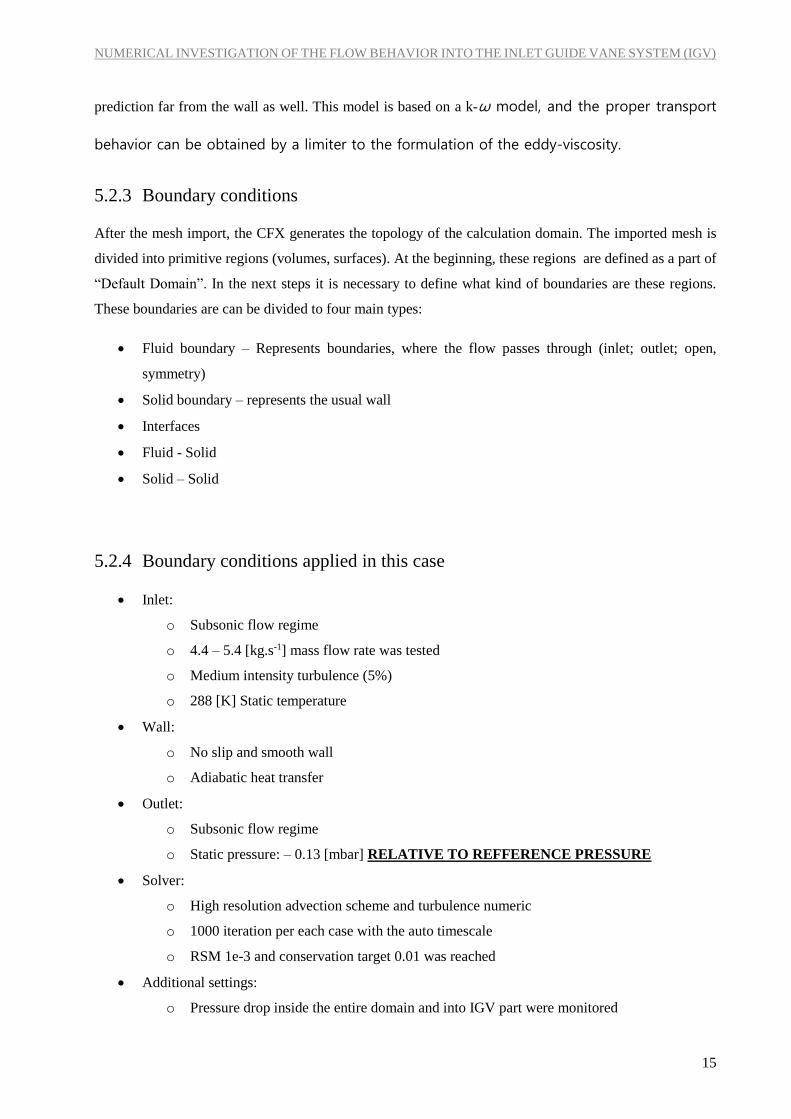
5.2.4 Boundary conditions applied in this case
Inlet:
o Subsonic flow regime
o 4.4 – 5.4 [kg.s-1] mass flow rate was tested
o Medium intensity turbulence (5%)
o 288 [K] Static temperature
Wall:
o No slip and smooth wall
o Adiabatic heat transfer
Outlet:
o Subsonic flow regime
o Static pressure: – 0.13 [mbar] RELATIVE TO REFFERENCE PRESSURE
Solver:
o High resolution advection scheme and turbulence numeric
o 1000 iteration per each case with the auto timescale
o RSM 1e-3 and conservation target 0.01 was reached
Additional settings:
o Pressure drop inside the entire domain and into IGV part were monitored
Page 17
NUMERICAL INVESTIGATION OF THE FLOW BEHAVIOR INTO THE INLET GUIDE VANE SYSTEM (IGV)
16
Fig. 9 Boundary conditions for the IGV channel
Page 18
NUMERICAL INVESTIGATION OF THE FLOW BEHAVIOR INTO THE INLET GUIDE VANE SYSTEM (IGV)
17
6 RESULTS
6.1 SOLVER AND ARRANGEMENT OF THE FILES
The calculation was evaluated by ANSYS CFD-POST ver. 14.0. Result files are situated in
IGV/CALCULATIONS/RESULTS folder. There are another subfolders inside the “RESULTS” folder.
Numbers indicate the current mass flow rate of e.g. 5_0 it means 5.0 [kg.s-1].
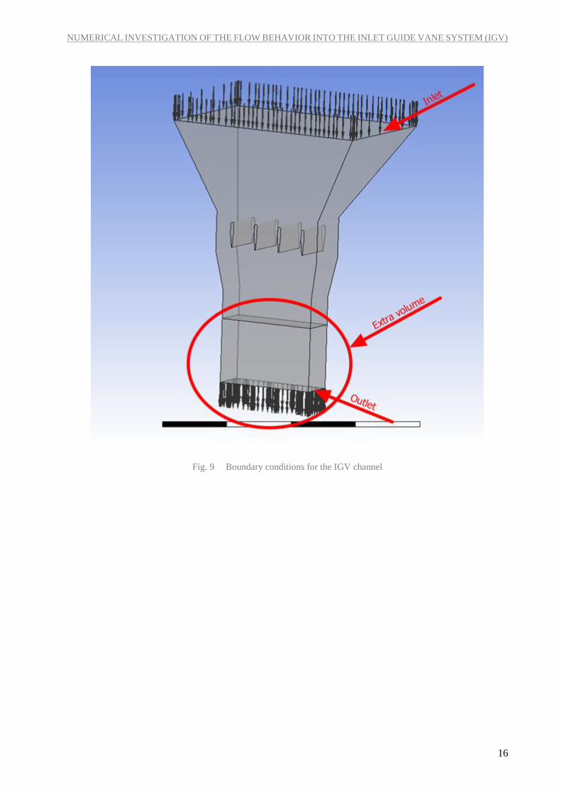
6.2 INVESTIGATED PARAMETERS
The main goal of this project was to investigate:
Pressure drop generated by the IGV with a different blade position and with a different mass flow
rate.
o Investigation at the measurement point
o Investigation at the plane which is situated at the same level as the measurement point is
situated
o Investigation along the wall, where the measuring device is situated
Investigation of the flow behavior inside the channel
Evaluated areas are displayed in the Fig. 10.
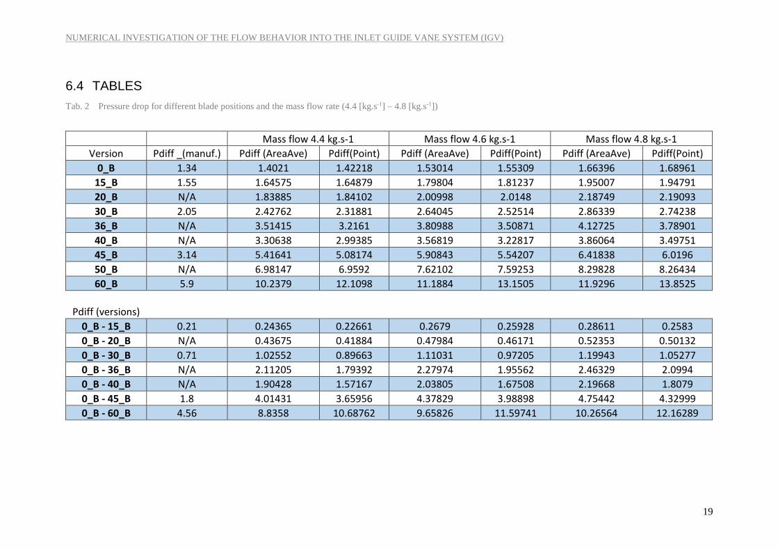
6.3 TABLES DESCRIPTION
The first column (from left) displays which position of IGV blades is investigated 0_B = 0 angle;
blended inlet
The second “Pdiff(manuf.)” part indicates the pressure drop given by the manufacturer
Pdiff (AreaAve) – Indicates the pressure drop:
o Area averaged static pressure at “Inlet” - Area averaged static pressure at “Measuring
Plane”
Pdiff (Point) – Indicates the pressure drop:
o Area averaged static pressure at “Inlet” - Static pressure at “Measuring Point”
Pdiff (versions) – Indicates the difference of values of the Pdiff (AreaAve) and the Pdiff (Point)
between different blade positions.
Page 19
NUMERICAL INVESTIGATION OF THE FLOW BEHAVIOR INTO THE INLET GUIDE VANE SYSTEM (IGV)
18
Fig. 10 Evaluated areas
Page 20
NUMERICAL INVESTIGATION OF THE FLOW BEHAVIOR INTO THE INLET GUIDE VANE SYSTEM (IGV)
19
6.4 TABLES
Tab. 2 Pressure drop for different blade positions and the mass flow rate (4.4 [kg.s-1] – 4.8 [kg.s-1])
Mass flow 4.4 kg.s-1 Mass flow 4.6 kg.s-1 Mass flow 4.8 kg.s-1
Version Pdiff _(manuf.) Pdiff (AreaAve) Pdiff(Point) Pdiff (AreaAve) Pdiff(Point) Pdiff (AreaAve) Pdiff(Point)
0_B 1.34 1.4021 1.42218 1.53014 1.55309 1.66396 1.68961
15_B 1.55 1.64575 1.64879 1.79804 1.81237 1.95007 1.94791
20_B N/A 1.83885 1.84102 2.00998 2.0148 2.18749 2.19093
30_B 2.05 2.42762 2.31881 2.64045 2.52514 2.86339 2.74238
36_B N/A 3.51415 3.2161 3.80988 3.50871 4.12725 3.78901
40_B N/A 3.30638 2.99385 3.56819 3.22817 3.86064 3.49751
45_B 3.14 5.41641 5.08174 5.90843 5.54207 6.41838 6.0196
50_B N/A 6.98147 6.9592 7.62102 7.59253 8.29828 8.26434
60_B 5.9 10.2379 12.1098 11.1884 13.1505 11.9296 13.8525
Pdiff (versions)
0_B - 15_B 0.21 0.24365 0.22661 0.2679 0.25928 0.28611 0.2583
0_B - 20_B N/A 0.43675 0.41884 0.47984 0.46171 0.52353 0.50132
0_B - 30_B 0.71 1.02552 0.89663 1.11031 0.97205 1.19943 1.05277
0_B - 36_B N/A 2.11205 1.79392 2.27974 1.95562 2.46329 2.0994
0_B - 40_B N/A 1.90428 1.57167 2.03805 1.67508 2.19668 1.8079
0_B - 45_B 1.8 4.01431 3.65956 4.37829 3.98898 4.75442 4.32999
0_B - 60_B 4.56 8.8358 10.68762 9.65826 11.59741 10.26564 12.16289
Page 21
NUMERICAL INVESTIGATION OF THE FLOW BEHAVIOR INTO THE INLET GUIDE VANE SYSTEM (IGV)
20
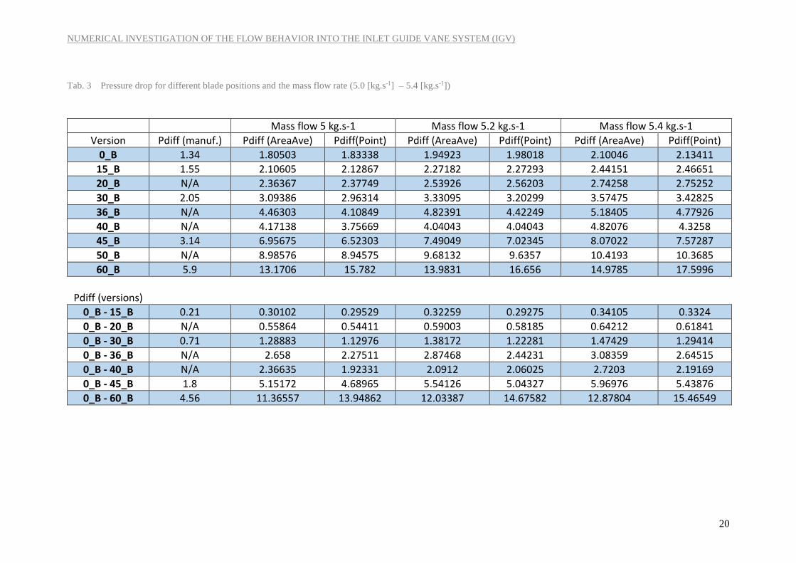
Tab. 3 Pressure drop for different blade positions and the mass flow rate (5.0 [kg.s-1] – 5.4 [kg.s-1])
Mass flow 5 kg.s-1 Mass flow 5.2 kg.s-1 Mass flow 5.4 kg.s-1
Version Pdiff (manuf.) Pdiff (AreaAve) Pdiff(Point) Pdiff (AreaAve) Pdiff(Point) Pdiff (AreaAve) Pdiff(Point)
0_B 1.34 1.80503 1.83338 1.94923 1.98018 2.10046 2.13411
15_B 1.55 2.10605 2.12867 2.27182 2.27293 2.44151 2.46651
20_B N/A 2.36367 2.37749 2.53926 2.56203 2.74258 2.75252
30_B 2.05 3.09386 2.96314 3.33095 3.20299 3.57475 3.42825
36_B N/A 4.46303 4.10849 4.82391 4.42249 5.18405 4.77926
40_B N/A 4.17138 3.75669 4.04043 4.04043 4.82076 4.3258
45_B 3.14 6.95675 6.52303 7.49049 7.02345 8.07022 7.57287
50_B N/A 8.98576 8.94575 9.68132 9.6357 10.4193 10.3685
60_B 5.9 13.1706 15.782 13.9831 16.656 14.9785 17.5996
Pdiff (versions)
0_B - 15_B 0.21 0.30102 0.29529 0.32259 0.29275 0.34105 0.3324
0_B - 20_B N/A 0.55864 0.54411 0.59003 0.58185 0.64212 0.61841
0_B - 30_B 0.71 1.28883 1.12976 1.38172 1.22281 1.47429 1.29414
0_B - 36_B N/A 2.658 2.27511 2.87468 2.44231 3.08359 2.64515
0_B - 40_B N/A 2.36635 1.92331 2.0912 2.06025 2.7203 2.19169
0_B - 45_B 1.8 5.15172 4.68965 5.54126 5.04327 5.96976 5.43876
0_B - 60_B 4.56 11.36557 13.94862 12.03387 14.67582 12.87804 15.46549
Page 22
NUMERICAL INVESTIGATION OF THE FLOW BEHAVIOR INTO THE INLET GUIDE VANE SYSTEM (IGV)
21
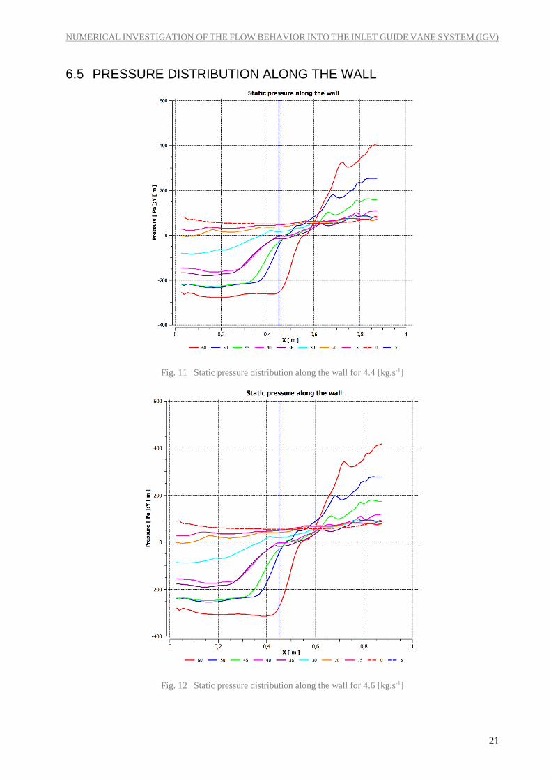
6.5 PRESSURE DISTRIBUTION ALONG THE WALL
Fig. 11 Static pressure distribution along the wall for 4.4 [kg.s-1]
Fig. 12 Static pressure distribution along the wall for 4.6 [kg.s-1]
Page 23
NUMERICAL INVESTIGATION OF THE FLOW BEHAVIOR INTO THE INLET GUIDE VANE SYSTEM (IGV)
22
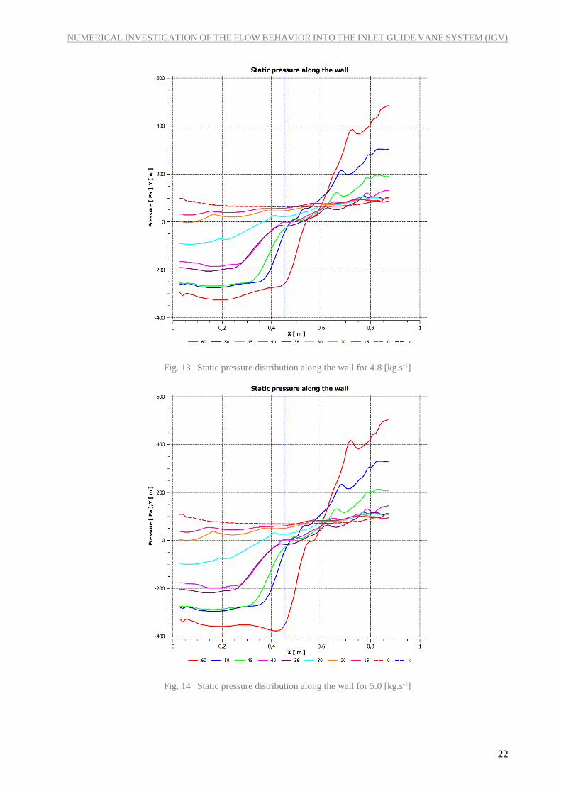
Fig. 13 Static pressure distribution along the wall for 4.8 [kg.s-1]
Fig. 14 Static pressure distribution along the wall for 5.0 [kg.s-1]
Page 24
NUMERICAL INVESTIGATION OF THE FLOW BEHAVIOR INTO THE INLET GUIDE VANE SYSTEM (IGV)
23
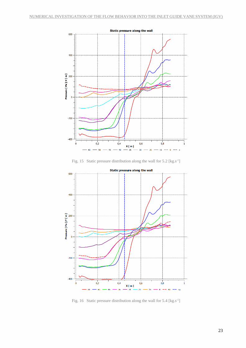
Fig. 15 Static pressure distribution along the wall for 5.2 [kg.s-1]
Fig. 16 Static pressure distribution along the wall for 5.4 [kg.s-1]
Page 25
NUMERICAL INVESTIGATION OF THE FLOW BEHAVIOR INTO THE INLET GUIDE VANE SYSTEM (IGV)
24
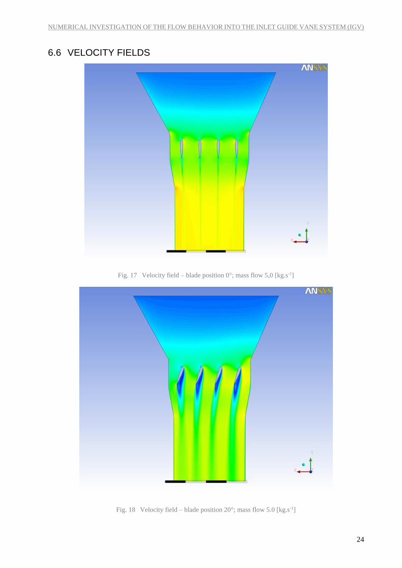
6.6 VELOCITY FIELDS
Fig. 17 Velocity field – blade position 0°; mass flow 5,0 [kg.s-1]
Fig. 18 Velocity field – blade position 20°; mass flow 5.0 [kg.s-1]
Page 26
NUMERICAL INVESTIGATION OF THE FLOW BEHAVIOR INTO THE INLET GUIDE VANE SYSTEM (IGV)
25
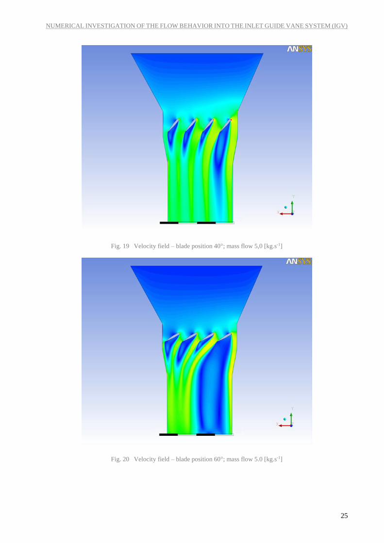
Fig. 19 Velocity field – blade position 40°; mass flow 5,0 [kg.s-1]
Fig. 20 Velocity field – blade position 60°; mass flow 5.0 [kg.s-1]
Page 27
NUMERICAL INVESTIGATION OF THE FLOW BEHAVIOR INTO THE INLET GUIDE VANE SYSTEM (IGV)
26
7 CONCLUSIONS
This calculation was focused to investigate the behavior of the IGV system. The calculation showed the
evolution of the pressure drop and its distribution along the IGV system. There are several conclusions
from the results:
The pressure drop behavior is according to the expectation. The pressure drop is changing
according to the angle of the rotation of the blades and the mass flow rate (Tab. 2; Tab. 3)
The difference between the values of measurement at the laboratory is very promising.
The calculated values of a pressure drop are more pessimistic than the measured data. Which can
be caused by an absence of the lower part, where the compressor is not included, or bad boundary
conditions, Fig. 8
The calculation revealed that the pressure distribution under the IGV blades is not homogenous
(Fig. 11 – Fig. 16). When the blade rotates, one side creates a tapering channel and the other a
diffuser channel (Fig. 17 – Fig. 20). These channels have a high effect to the pressure distribution
and its effect increases with higher angles of the blade position.
7.1 SUGGESTIONS FOR FURTHER WORK
To implement the lower part of the IGV into the numerical investigation, with a compressor, and
to improve boundary conditions
To redesign the measurements of the pressure drop