NUMERICAL INVESTIGATIONS OF A TORNADO VORTEX USING VORTICITY CONFINEMENT

by

HOLLY C. HASSENZAHL

A thesis submitted in partial fulfillment of the requirements for the degree of

Master of Science (Atmospheric and Oceanic Sciences)

at the

UNIVERSITY OF WISCONSIN MADISON

2007

i

ABSTRACT

The numerical simulation of a realistically strong tornado vortex and its associated

condensation funnel has proven to be very difficult to resolve in atmospheric modeling.

Many have attributed this failure to insufficient resolution of the models being used. Others

have conjectured that the problem lies in the fact that strong gradients are eroded by

numerical diffusion, thus prohibiting the formation of strong vortices. This latter hypothesis

led engineers Steinhoff and Underhill (1994) to conceive the Vorticity Confinement (VC)

technique, in an effort to restore the vorticity gradients lost to diffusion. In this study, the

University of Wisconsin Non-Hydrostatic Modeling System (UW-NMS) is used to

investigate the aforementioned hypotheses on a three-dimensional extension of the Wicker

and Wilhelmson (1995) tornado vortex. These idealized simulations are carried out with

two-way interactive nested grids at horizontal resolutions of 24 m and 12 m. Simulations

without the VC technique do produce tornado vortices at both resolutions, however they are

too weak to form condensation funnels extending to the surface. Comparisons with

simulations employing the VC technique show that a realistically strong tornado vortex is

resolved at the 24 m resolution, producing a beautiful condensation funnel that descends to

the ground. However, when extended to a resolution of 12 m, the VC technique fails to

converge to the real solution. At this high resolution, the vortex spins-up at an unrealistic

pace, having an extremely large magnitude of vorticity and a very small diameter. It is

conjectured that the problem lies in the absence of an explicit energy budget in the VC

formulation. Without this budget, there are no physical constraints on the energy added into

the system by the confinement term.

ii

An additional experiment is performed to investigate the role of centrifuging rain

droplets on tornado vortex intensity. A UW-NMS simulation using the VC technique at 24

m resolution is run without centrifugal force acting on the rain droplets and then compared to

the original VC simulation at the same resolution. Results show that the centrifuging of rain

droplets has the net effect of intensifying the tornado vortex over time. As droplets are

thrown out of the vortex, they exert a drag force on the surrounding air. This effectively

removes mass from within the tornado, reducing the inside pressure and therefore increasing

the pressure gradient force. Convergence and wind speeds in the vortex are thereby

enhanced, stretching the vortex and further increasing the vertical vorticity.

iii

TABLE OF CONTENTS

Abstract ...................................................................................................................................... i

1. Introduction..........................................................................................................................1

2. Background and Literature Review .....................................................................................3

2.1. Numerical Simulation of Tornadoes.............................................................................3

2.2. Vorticity Confinement Theory .....................................................................................5

2.3. Centrifuging of Hydrometeors in a Vortex...................................................................9

3. Experiment Design.............................................................................................................14

3.1. Numerical Model ........................................................................................................14

3.1.1. Governing Equations .......................................................................................14

3.1.2. Physical Parameterizations ..............................................................................17

3.1.3. Boundary Conditions .......................................................................................18

3.1.4. ..Finite Differencing...........................................................................................19

3.1.5. Vorticity Confinement Methodology...............................................................21

3.2. Model Initialization ....................................................................................................24

4. Discussion of Results.........................................................................................................28

4.1. Evolution of Wicker and Wilhelmson Tornado Vortices ...........................................28

4.1.1. Evolution of a Single Tornado Vortex at Higher Resolution ..........................34

4.2. Effects of Vorticity Confinement ...............................................................................36

4.3. Effects of Centrifuging Rain Droplets ........................................................................41

5. Conclusion .........................................................................................................................88

Appendix..................................................................................................................................90

References................................................................................................................................95

1

Chapter 1

Introduction

The numerical simulation of tornado development must first begin with the successful

simulation of the parent thunderstorm from which it forms. The most likely storm to

generate tornadic activity is the supercell, characterized by a single, rotating updraft that

ascends into the thunderstorm on a tilted path. This path makes it difficult for downdrafts

that form within the thunderstorm to interfere with the energy-providing updraft. The end

result is a powerful, rotating thunderstorm with an extremely long life-span and the

heightened potential for tornado development.

Roughly 30 years ago cloud modelers began making achievements in the numerical

simulation of supercell thunderstorms and their observed features (Schlesinger 1978, 1980;

Wilhelmson and Klemp 1978, 1981; Klemp and Wilhelmson 1978a, 1978b; Weisman and

Klemp 1982, 1984; Tripoli and Cotton 1986). Thus, the groundwork was laid for future

experiments involving the formation of a tornado vortex within the mesocyclone of a

supercell (Klemp and Rotunno, 1983; Wicker, 1990; Grasso and Cotton, 1995; Wicker and

Wilhelmson, 1995). However, these experiments were only partially successful in that they

simulated the small-scale features associated with tornadoes, but failed to resolve a vortex

strong enough to produce the tornado itself. The modeling community attributed this failure

to the insufficient resolution of the models being used. However, recent results from Tripoli

et al. (2004) have shown that even at very high resolution, a sufficiently strong tornado

vortex will not develop in a numerical model. Steinhoff and Underhill (1994) suggest that

the problem lies in the numerical diffusion of the model, which acts to weaken tight gradients

2

in fluid flow. In an effort to alleviate this problem in the engineering community, they

developed a technique that seeks to restore the gradient of vorticity lost to numerical

smoothing. Following positive results in many areas of fluid flow modeling, a modified

version of this Vorticity Confinement technique was developed specifically for use in

atmospheric modeling.

Therefore, it is the goal of this thesis to evaluate the performance of the modified

Vorticity Confinement (VC) technique. This research began by first extending the Wicker

and Wilhelmson (1995) idealized simulation of a tornadic supercell by performing the

experiments at higher resolution. The modified VC technique was then employed on the

high-resolution simulations in order to study its effects on the development of the tornado

vortex and its condensation funnel.

Following these experiments, further research was performed in order to study the

effect that centrifuged rain droplets have on the strength of the tornado vortex. The impetus

for this work came from the fact that rain droplets exert a drag force on the surrounding air as

they are centrifuged, or thrown out, from inside a vortex. Dragging air with them, the

droplets remove mass from within the vortex, leading to a decrease in the central pressure

and an overall intensification of the tornado. To test this theory, the centrifugal force acting

on rain droplets was neglected in the model.

Background information detailing previous modeling experiments is presented in

Chapter 2. The numerical model used in this work, as well as the modified version of the VC

technique are both discussed in Chapter 3. Results from the various experiments performed

are presented in Chapter 4, with concluding remarks given in Chapter 5.

3

Chapter 2

Background and Literature Review

2.1 Numerical Simulation of Tornadoes

Following the success of large-scale simulations of supercell thunderstorms, Klemp

and Rotunno (1983, hereafter referred to as KR83) sought out to simulate the smaller scale

features that develop in conjunction with the formation of a tornado within a mature

supercell. To perform this experiment, KR83 used a one-way nested model with the

innermost grid having a horizontal resolution of 250 meters and a vertical grid spacing of 500

m. The fine grid was centered over the main circulation of the previously simulated 20 May

1977 Del City tornadic supercell (Klemp et al. 1981). The experiment proved to accurately

resolve several of the small-scale features observed within tornadic thunderstorms, but failed

to produce the tornado itself. However, analysis of their results led to the conclusion that

vertical vorticity at low levels is achieved through the tilting of baroclinically produced

horizontal vorticity near the intersection of the updraft and the forward flank downdraft.

Once this vertical vorticity was achieved by KR83, its circulation quickly intensified as a

result of the enhanced convergence at low-levels. In turn, the intense low-level circulation

strengthened the rear flank downdraft. The KR83 results thus proved that with sufficiently

small grid spacing, numerical models can successfully resolve many small scale features that

occur in association with the tornadic phase of the supercell life-cycle.

4

Wicker’s 1990 Ph.D. thesis (hereafter referred to as W90) extended the work of

Wilhelmson and Klemp (1981) on the 3 April 1964 supercell through the analysis of fine-

scale features within the storm. The fine mesh in this experiment had a resolution of 70 m in

the horizontal with a 50 m vertical resolution at the surface, accomplished by way of a

vertically stretched grid. A distinct vortex with a several-minute life span was achieved

within the broader circulation of the mesocyclone. The magnitude of maximum vorticity

within the tornado vortex reached 0.35 s-1

. While the work of KR83 and W90 produced

encouraging results, they were indeed limited by the computational abilities of the time these

experiments were performed. The short time periods over which the fine grids could be

integrated meant they could not be initialized well in advance of the vortex genesis, leaving

the initial development phase difficult to analyze. Thus in order to accurately resolve the full

evolution of a tornado vortex, a sufficiently high resolution simulation must be carried out

over a time period that encompasses the pre-tornadic environment.

Wicker and Wilhelmson (1995, hereafter referred to as WW95) thereby extended the

work of KR83 and W90 by using a two-way interactive adaptive grid system to simulate

tornado development at very high resolution and over much longer time periods. With the

ability to initialize the innermost grid 10-15 minutes prior to the maximum in vortex

intensity, ample time was given for flow adjustments to be made in response to the increased

resolution. The coarse grid used in WW95 had a horizontal resolution of 600 m with vertical

resolution of 120 m at the surface, stretching to 700 m at 7.5 km. The fine mesh employed

120 m horizontal grid spacing, while keeping the vertical grid spacing identical to that of the

coarse grid. The fine mesh was initialized 70 minutes into the simulation and was integrated

forward for 40 minutes. During that time, the development of two distinct tornado vortices

5

occurred, as determined by a marked decrease in surface pressure. The first tornado vortex

reached its peak 87 minutes into the simulation, while the second vortex peaked at 102

minutes. Each development phase lasted approximately 8 to 10 minutes, with ground-

relative surface wind speeds surpassing 60 m s-1

.

The strongest resolved tornado vortex was achieved by Xue (2004), using a terascale

system from the Pittsburgh Supercomputing Center. Given the enormous computing power,

Xue was able to encompass the entire supercell in a single 50 km by 50 km domain with 25

m horizontal resolution and 20 m vertical resolution at the surface. This is the largest

numerical simulation of a tornado that has been performed to date. The experiment resulted

in a realistic tornado life cycle with an 80 hPa drop in pressure and wind speeds exceeding

120 m s-1

(F5 tornado). However, Xue has yet to publish a full documentation of this

research, so many of the factors that went into the model are currently unknown.

While there have clearly been large advances in the numerical simulation of

tornadoes, resolving a realistically strong vortex that produces a condensation funnel has

proven difficult. One suggested reason and potential solution for this problem are discussed

in the following section.

2.2 Vorticity Confinement Theory

In all scales of atmospheric flow, there exist fields in which extremely strong

gradients or discontinuities can occur. For example, temperature gradients within a frontal

zone can tighten to become a first or zeroeth order discontinuity. The tropopause is a first

order discontinuity in entropy and a zeroeth order discontinuity in potential vorticity. The

6

interface between the warm, moist updraft and the cold downdraft of a thunderstorm is also a

zeroeth order discontinuity and plays a highly important role in storm dynamics and

evolution. Even though these locally extreme gradients occur in nature, they are very

difficult to resolve in a numerical model using the Eulerian framework. The Eulerian form of

the momentum equations gives us the local change of momentum, mass and entropy which

are determined using spatial derivatives defined by the model. As gradients collapse to a

zeroeth order discontinuity, the accuracy of the numerical solution significantly decreases as

these gradients are forced to become more diffuse in order to be resolved by the model. This

shortcoming is especially noticeable when attempting to model small scale vortices in the

atmosphere, such as tornadoes, where a zeroeth order vorticity gradient occurs along the edge

of the vortex. Numerical dissipation of vorticity reduces this gradient, making it impossible

for the simulated vortex to realistically intensify.

The problem of unresolved small scale vortices in numerical simulations is not unique

to atmospheric sciences. Engineers have long struggled with this issue when attempting to

accurately simulate such things as flow separation, vortex shedding and shock propagation in

both fluid and air as they flow around obstacles. Seeking to alleviate the problem of

unresolved small scale vortices in the numerical simulation of vortex-shedding by aircraft

wings, Steinhoff and Underhill (1994, hereafter referred to as SU94) developed the Vorticity

Confinement (VC) technique. The driving theory behind this technique comes from the idea

that vorticity is confined by the inertial stability of the vortex. As inertial stability builds, it

blocks the downward turbulent cascade of vorticity at some scale, thus protecting the vortex

from loss of energy to lower scales in the spectrum. Despite great advances in numerical

modeling, even the most eloquent numerical schemes employed today are unable to resolve

7

this natural confinement of vorticity. Instead, scales are truncated through numerical

smoothing, permitting the loss of energy through the bottom of the spectrum and inhibiting

the formation of a strong vortex. Thus the goal of the VC technique is to artificially restore

the strong vorticity gradients lost to numerical smoothing at the appropriate grid scale. This

is done by preserving the physical structure of both vortex filaments and vortex sheets, or

what SU94 calls “the essential features of small scale vortices.”

Vorticity confinement is unique in that it is not based on one-dimensional

compressible flows, as were previous methods like that of Smolarkiewicz and Margolin

(1993). In addition, VC is designed to be rotationally invariant and independent of the basic

equations of motion, thus making it a simple addition to present atmospheric models. Over

the last decade, the VC technique has been applied to numerous fluid flow problems within

the engineering community. The results have been positive as small scale physical structures

are preserved in the various flow regimes, creating more realistic simulations. Fan et al.

(2002) employed the VC technique for flow over round and square cylinders, as well as flow

over a helicopter landing ship. For the cases of flow over the cylinders, VC proved to rapidly

and accurately simulate the turbulent wakes that develop behind these objects (Figure 2.1).

The simulations of flow across the deck of a helicopter landing ship showed that vortices that

develop on the windward side of the ship were far less dissipated and much longer lasting

than those produced when not using VC (Figure 2.2).

In recent years, the VC technique has been embraced by the computer graphics

community, especially those modeling natural phenomena such as smoke plumes, water

eddies, cumulus clouds, and tornadoes. Fedkiw et al. (2001) used VC to more accurately

simulate and visualize smoke. It was shown that by using this confining technique, the

8

model was able to resolve the small scale rolling features typically observed in regions of

smoke. Miyazaki et al. (2002) employed VC in their simple atmospheric model in order to

create convincing animations of the development, advection and dissipation of cumulus and

cumulonimbus clouds for use in outdoor scenes. In order to accurately resolve these

cumuliform clouds, small scale turbulent vortices must be protected from numerical

dissipation. VC was shown to do just that, giving Miyazaki et al. more detailed and realistic

cloud images and animations.

Since 2004, Tripoli et al. (2004, 2006) have been working with the VC technique in

atmospheric modeling. Upon observing the formation of waterspouts while on a ship in the

Tyrrhenian Sea between Italy and Corsica, Tripoli and a few of his colleagues set out to

explicitly simulate the event. The University of Wisconsin Non-Hydrostatic Modeling

System (UW-NMS) designed by Tripoli (1992, 2007) was employed for these experiments

using a two-way interactive grid with very high-resolution capabilities. The finest mesh of

the simulation was the eighth grid having a horizontal grid spacing of only 2 m. This grid

was centered over a strong vortex that had developed along a shear line in the coarser grids.

A weak waterspout was achieved with only a 1-4 hPa drop in pressure at the core of the

vortex. A condensation funnel began to form but extended only slightly below the cloud

base. The resolution of this simulation, being much higher than previous experiments,

proved that simply increasing the model resolution was not enough to resolve realistically

strong vortices, as assumed by the tornado modeling community. After employing the VC

technique, the waterspout developed into a much stronger vortex with a 35-40 hPa pressure

drop at the core and a condensation funnel descending to 400 m below the cloud base. These

9

results were far more realistic, matching up quite well to the waterspout event observed in the

Tyrrhenian Sea.

While the results of Tripoli et al. were exciting and promising, the question remained

as to whether the methodology behind VC was truly physical or simply a technique better

used for special effects in Hollywood. After much study, Tripoli concluded that a more

scientifically defensible form of VC could be achieved. As discussed by Lilly (1986), a

balanced vortex naturally opposes the erosion due to physical turbulence. Thus the modified

VC technique estimates the amount of dissipation of the three-dimensional vorticity gradient

by numerical smoothers, only. The vorticity is then restored through an up-gradient source

term equal to the estimated loss incurred by the smoothers. This source term, or anti-

diffusion velocity, differs from the original SU94 formulation in that its magnitude is

dependent on the fraction of vorticity in dynamic balance. The derivation of this modified

VC term is given in Section 3.1.5.

2.3 Centrifuging of Hydrometeors in a Vortex

Visual and radar observations of waterspouts and tornadoes have shown there to be a

hollow structure to these vortices. In an attempt to explain this phenomenon, Kangieser

(1954) conducted experiments using a Rankine combined vortex model. Results showed that

when foreign particles enter a vortex an inward-directed drag force and an outward-directed

centrifugal force are exerted on them. These two forces balance each other at an equilibrium

distance from the center of the vortex, as determined by the size and fall speed of the particle.

An annulus of particles forms at this equilibrium radius, with larger and denser particles

10

being further from the vortex center and smaller particles being closer. In a steady-state

vortex, these particles will travel at a constant velocity, following a circular path around the

vortex. Thus a hollow tube is achieved at the vortex core due to the centrifuging, or outward

movement, of particles as they seek a balanced state.

In recent decades, advances in radar technology have made it possible to achieve

detailed and often up-close observations of tornado structure. Hence, an increasing amount

of observations have been noted in the literature regarding the centrifuging of hydrometeors

and debris particles by a tornado vortex (Wakimoto and Martner 1992; Bluestein et al. 1993;

Wurman et al. 1996; Wurman and Gill 2000; Dowell and Bluestein 2002; Burgess et al.

2002).

Of particular significance is the work of Dowell et al. (2005) in which the behavior of

hydrometeors and other foreign debris particles inside a tornado vortex was studied. Part of

this research was conducted using idealized one-dimensional and two dimensional numerical

simulations of axisymmetric Rankine vortices. The results confirmed those of Kangieser

(1954) showing that denser particles with larger fall speeds have slower tangential wind

speeds than the air in the vortex and are thus centrifuged outward away from the vortex core.

The radial velocity of this outward motion with respect to the air increased with the

increasing size and fall speed of the particle. For small rain droplets with fall speeds of 2 m

s-1

, the radial velocities ranged between 3 and 7 m s-1

, depending on the size and strength of

the vortex. This range was found to be 12 to 28 m s-1

in the case of large raindrops or small

hailstones with fall speeds of 10 m s-1

. It should be noted that the relative air speed of

particles that are simultaneously falling and being centrifuged is larger than if they were

simply falling through calm air. Thus, particle fall speeds were largely reduced inside the

11

simulated vortices, allowing the much larger radial velocities to eject the particles

horizontally outward at small angles. Of particular importance to the research discussed in

this paper was the finding that the centrifuging of hydrometeors and other particles greatly

reduced their number concentration inside the vortex, while raising it outside (Figure 2.3).

Experiments to assess the impact of this centrifuging on the strength of the vortex are

discussed in Section 4.2.2.

12

(a) (b)

Figure 2.1: Isosurface of vorticity for flow over a cylinder (a) without vorticity confinement

and (b) with vorticity confinement. From Fan et al. (2002).

(a) (b)

Figure 2.2: Isosurface of vorticity for flow over the windward side of a helicopter landing

ship (a) without vorticity confinement and (b) with vorticity confinement. Windward side

corresponds to the bottom of the figures. From Fan et al. (2002).

13

Figure 2.3: Radial profiles every 10 seconds of the number concentration of small raindrops

(terminal fall speeds of -2 m s-1

) within a Rankine vortex of radius 100 m and with tangential

velocities of 100 m s-1

at the edge.

14

Chapter 3

Experiment Design

3.1 Numerical Model

All experiments for this research were conducted using the University of Wisconsin

Non-Hydrostatic Modeling System (UW-NMS). The UW-NMS is a three-dimensional, non-

hydrostatic model whose enstrophy and kinetic energy conserving design allows for greater

accuracy in simulating multi-scale interactions. Some of the key features of this model

include modifiable grid size and resolution in both the horizontal and vertical, multiple two-

way interactive grid nesting with moveable inner grids, and grid-scale microphysics

parameterization with cloud water, rain, pristine crystals, snow, aggregate crystals and

graupel. The UW-NMS design is fully described by Tripoli (1992) and Tripoli (2007).

3.1.1 Governing Equations

3.1.1.1 Equations of Motion

For simplicity, the enstrophy-conserving form of the equations of motion may be

given by the following:

gFFSIGBt

uiiiiiiu

i

3

21 δ−+++=+∂

∂ (3.1)

where BuGi are the pressure gradient accelerations, Ii are the inertial accelerations, Si are

sources of momentum, 1

iF represents turbulent mixing tendencies, 2

iF is the velocity

15

tendency from a numerical filter which controls noise and aliasing in the model, δij is the

Kronecker delta, and g is gravitational acceleration,

The pressure gradient accelerations include a buoyancy coefficient in addition to the

pressure gradients. The terms are defined as follows:

Bu = θvv (3.2)

i

ix

G∂

∂=

π (3.3)

The variable θvv in (3.2) is the water loading virtual potential temperature, and is

defined as:

)1()1(

)61.01(

iceliq

v

iceliq

v

vvqqqq

q

++=

++

+=

θθθ (3.4)

where qv, qliq, and qice are the specific masses of vapor, liquid and ice, respectively, θ is

potential temperature and θv is virtual potential temperature. The variable, π, in (3.3) is the

Exner function and is related to pressure, p, by the following equation:

pcR

oo

pp

pc

/

=π (3.5)

where cp is the specific heat of dry air when p is held constant, R is the gas constant for dry

air, and poo = 1000hPa.

The enstrophy-conserving inertial accelerations are defined as follows:

i

kjkjiix

kmI

∂

∂−= ηε ,, (3.6)

where the momentum vector, mi, is given by:

.cosφρ iTi um = (3.7)

16

The total air density, ρT, is defined to be:

)1)(()1( iceliqvdiceliqT qqqq +++=++= ρρρρ (3.8)

where ρ represents the total density of air and water combined (ρd + ρv).

The three components of absolute vorticity per unit mass, ηi, is defined as:

φρ

ςη

cosT

ii

i

f+= (3.9)

where fi represents the three components of the Coriolis force, and ζi represents the three

components of relative vorticity, given to be:

i

j

kjiix

u

∂

∂= ,,ες (3.10)

The specific kinetic energy, k, is defined as:

euk i3

2)(

2

1 2 += (3.11)

The variable, e, represents the turbulent kinetic energy (TKE). The NMS model may be set

to either diagnose or explicitly predict TKE. This will be discussed further in the following

section.

As seen from the above equations, velocity tendency is made up of balances among

inertial, pressure gradient and gravitational forces. As shown by Equation (3.9), all rotational

accelerations are linked together into a single vorticity term. The residual inertial

acceleration term is depicted as a gradient in kinetic energy, seen in Equation (3.6). It is

worth noting that this particular system is only applicable for meso-β-scale flows or smaller,

where the system is integrated on an f plane and curvature may be neglected (Tripoli, 1992).

17

3.1.2 Physical Parameterizations

The generic tendency equation used for the highly conservative variables in the model

is given by:

AAAAA SFFPIt

A++++=

∂

∂ 21 (3.12)

where A is the conserved scalar variable being predicted, IA represents the inertial tendencies

of advection, PA is the precipitation settling, 1

AF represents physical turbulence mixing which

is based on a physical closure scheme, 2

AF is a numerical filter and SA is a general source term

that represents all remaining sources of the variable A.

The turbulence closure scheme used for the experiments in this paper is one in which

the turbulent kinetic energy is diagnosed, as described by Redelsperger and Someria (1982)

for their level one closure. In this scheme, turbulent kinetic energy, e, is assumed to be

following a Lagrangian trajectory while in steady state balance. Thus the individual terms

that comprise Se in Equation (3.12) become such that Se = 0 locally.

The UW-NMS uses a selective filter in order to control nonlinear instability and

numerical noise. The generic form of the equation is given by:

Azz

FAyy

FAxx

FF

vhhn

oV

n

H

n

HA′

∂

∂

∂

∂+′

∂

∂

∂

∂+′

∂

∂

∂

∂=

2/2/2/

2 cos ρφ , (3.13)

where A is any variable for which there is a build up of numerically-induced small scale

variances, and nh and nv represent the order of the horizontal and vertical filters, respectively,

given in even integers.

Use of the numerical filter often results in the artificial transport of the variable, A. In

order to minimize this effect, the reference state may be subtracted from the scalar field that

18

is being smoothed by the filter, much like that described by Klemp and Wilhelmson (1978).

The fraction of maximum damping allowed is given by the horizontal and vertical filter

coefficients, FH and FV, shown in Equation (3.12). The value of the maximum damping is

based on the shortest wave produced by the model. For the experiments discussed in this

paper, the horizontal and vertical filter coefficients were set to 0.05 and 0.1, respectively, in

the outermost grid. The filter coefficients used in the finest grid were set to 0.1 for both the

horizontal and vertical. This increase in the fraction of maximum damping was required due

to the very high resolutions of the inner grids, leading to an increase of non-linear instability

in the model.

3.1.3 Boundary Conditions

3.1.3.1 Lateral Boundaries

The lateral boundaries in the idealized experiments employed the Klemp and

Wilhelmson gravity wave radiation condition (1978). This condition assumes that all inertial

terms are in balance with each other at the grid boundary, thus allowing gravity waves to

freely propagate out of the domain. The time tendency of velocity perpendicular to the

lateral boundaries of the grid is as follows:

x

uuc

t

u o

∂

−∂−=

∂

∂ )(* (3.14)

where o represents the initial state and c* is a Doppler-shifted phase speed for gravity waves,

written as:

c* = c + u (3.15)

19

where c is moving out of the domain. The Doppler-shifted phase speed used in the

experiments performed for this research was equal to 30 ms-1

.

3.1.3.2 Upper and Lower Boundaries

The upper boundary in these experiments was a wall with a Rayleigh friction zone

seven grid points deep. This friction zone was employed in order to absorb gravity waves as

they propagated toward the top of the model, avoiding improper reflection of the waves off

the upper boundary. The Rayleigh friction condition as defined by Clark (1977) is given by:

τ ′

−+

∂

∂=

′

∂

∂ )(oiiii

uu

t

u

t

u. (3.16)

The time scale, τ, is given through the following equation:

−

−=

′0,

)(

))(/1(max

1

FNZ

F

ZZ

ZZτ

τ (3.17)

where ZF represents the height of the bottom of the Rayleigh friction layer, and ZNZ

represents the model top height. For these experiments, τ = 120s.

The lower boundary of the model was free-slip and rigid. The surface layer scheme is

defined by Louis (1979) and provides specified turbulent fluxes of moisture, momentum and

heat. No soil or vegetation model was used.

3.1.4 Finite Differencing

The governing equations of the UW-NMS model are calculated on an Arakawa C-

grid (Arakawa, 1966). They are finite-differenced using a hybrid time-split, leapfrog-

forward, space-time scheme much like that described by Klemp and Wilhelmson (1978a) and

20

Tripoli (1992a). Figure 3.1 schematically summarizes how each advection term is finite-

differenced using this hybrid scheme. Since the dynamics equations are set up in an Exner

Function system, a smooth separation of the acoustic-containing fluctuations from the slower

inertial and gravitational fluctuations can occur. Thus a separate smaller time step can be

employed for the integration of the acoustic terms. A leapfrog scheme is applied to the

longer time-step of the inertial tendencies for velocity. These terms are finite-differenced in

a manner that best conserves enstrophy, kinetic energy and mean vorticity. A Crowley

forward scheme is employed for the integration of the scalar terms. This scheme is able to

achieve second-order accuracy while using information from only one time level. In

addition, the Crowley scheme in its flux-conserving form can be formulated to achieve

higher order accuracy.

For the purposes of this paper, in which vorticity confinement is the central focus,

special attention must be paid to the inertial momentum tendency (Ii). The finite differencing

of this particular advection term is done using the Arakawa and Lamb (1981, hereafter

referred to as AL81) scheme in which vorticity, kinetic energy, and enstrophy are conserved.

The AL81 scheme was modified so as to be used for three-dimensional, compressible flow

on grids where spacing may vary, as is the case in the UW-NMS model. The benefit of using

the AL81 scheme is that it removes numerical differencing biases that often result in the

artificial growth of the two-dimensional potential vorticity, specific kinetic energy and

enstrophy. As such, the modified, three-dimensional AL81 scheme can more accurately

simulate Ertel potential vorticity, which is simply defined as the dot product of the two-

dimensional potential vorticity and the gradient of entropy. Refer to Appendix 1 for the full

description of the modified AL81 scheme.

21

3.1.5 Vorticity Confinement Methodology

A series of experiments were conducted using a slightly modified version of the VC

scheme originally designed by Steinhoff and Underhill (1994, hereafter referred to as SU94).

As discussed in Chapter 2, the overarching aim of this scheme is to oppose the numerical

dissipation of vorticity in a balanced vortex by including in the momentum equations an

artificial up-gradient vorticity production term.

To derive this term, we first recall the equations of motion as given by Equation (3.1).

The term BuGi represents acceleration by the pressure gradient force, while Ii represents

inertial accelerations owing to vorticity and the kinetic energy gradient. From these terms we

can define three vectors that represent the pressure-gravity acceleration (A), the kinetic

energy gradient acceleration (B), and the total non-vorticity acceleration (C):

gGBt

uA iiu

gpg

i

3

,

δ−−=

∂

∂=

ikg

i

x

k

t

uB

∂

∂−=

∂

∂= (3.18)

BAt

uC

kggpg

i +=

∂

∂=

,,

We want the vorticity production term to be equal to a certain fraction of the

numerical dissipation of vorticity occurring in the model. This particular fraction should be

proportional to the amount of inertial vorticity acceleration that is being balanced by the total

non-vorticity acceleration, C:

Cu balg =×ς (3.19)

where balς represents the balanced portion of the vorticity defined as follows:

22

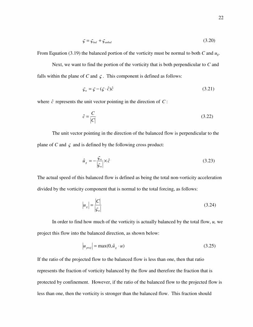
unbalbal ςςς += (3.20)

From Equation (3.19) the balanced portion of the vorticity must be normal to both C and ug.

Next, we want to find the portion of the vorticity that is both perpendicular to C and

falls within the plane of C and ς . This component is defined as follows:

ccnˆ)ˆ( ⋅−= ςςς (3.21)

where c represents the unit vector pointing in the direction of C :

C

Cc =ˆ (3.22)

The unit vector pointing in the direction of the balanced flow is perpendicular to the

plane of C and ς and is defined by the following cross product:

cun

n

gˆˆ ×−=

ς

ς (3.23)

The actual speed of this balanced flow is defined as being the total non-vorticity acceleration

divided by the vorticity component that is normal to the total forcing, as follows:

n

g

Cu

ς= (3.24)

In order to find how much of the vorticity is actually balanced by the total flow, u, we

project this flow into the balanced direction, as shown below:

)ˆ,0max( uuu gproj ⋅= (3.25)

If the ratio of the projected flow to the balanced flow is less than one, then that ratio

represents the fraction of vorticity balanced by the flow and therefore the fraction that is

protected by confinement. However, if the ratio of the balanced flow to the projected flow is

less than one, then the vorticity is stronger than the balanced flow. This fraction should

23

therefore not be protected by confinement. Thus, we reduce the confinement using the

following fraction:

=

proj

g

g

proj

u

u

u

u,,1min,0max1α (3.26)

We further limit the confinement of vorticity by considering only the portion of the total

acceleration, C, that is being forced by the pressure gradient and gravity, A. We do not

consider acceleration owing to the kinetic energy gradient, B, as it is an imaginary force.

Hence, VC is reduced by a second fraction determined as follows:

⋅

=C

cAr

ˆ,1min,0max2α (3.27)

The next step is to find the dissipation acceleration. We start with the linear

numerical diffusive flux, given by:

i

ii

ix

Ku∂

∂−=

ς

ς'''' (3.28)

where Ki is the linear mixing coefficient. It should be noted that physical turbulence is not

considered in Equation (3.28), only the numerical diffusion term. This is due to the fact that

physical turbulence already confines vorticity through its opposition to the deformation

fields. Using the linear numerical diffusive flux and the value of mean vorticity, we can now

find an effective diffusion velocity, Dur

, as follows:

=

ς

ς''''

i

D

uu (3.30)

24

The diffusion velocity is then projected onto c in order to calculate the confinement velocity.

This velocity is then reduced by the fractions, 1α and 2α , given by Equations (3.26) and

(3.27):

)ˆ,0max(21 cus D ⋅= αα (3.31)

and

css ˆ= (3.32)

The final step is to add the confinement velocity to the inertial acceleration term in

the momentum equations. Thus, Equation (3.6) becomes:

i

kkjjkjiix

kfsuI

∂

∂−++= ))((,, ςε (3.33)

3.2 Model Initialization

The UW-NMS model was initialized using an idealized thermodynamic profile

almost identical to that used in WW95. The horizontal wind profile in the vertical is also

modeled after the one used by Wicker and Wilhelmson. This idealized wind profile is based

on actual hodographs from tornadic storms in Binger, Oklahoma (Wicker et al. 1984),

Raleigh, North Carolina (Davies-Jones et al. 1990) and Davis, Oklahoma (Brown et al.

1973). The environment created by these profiles is conducive to supercell development,

with a convective available potential energy value of 4406 J kg-1

and a bulk Richardson

number of 43.7. This bulk Richardson number is slightly outside of the optimal range of 15-

35 for a right-moving supercell, as described by Weisman and Klemp (1982). However, the

value is within the broader range of 10-50, in which observations have shown the evolution

25

and strengthening of a right-moving supercell are still possible. The thermodynamic profile

and wind hodograph from WW95 are shown in Figure 3.2.

The thunderstorm is forced to initiate by imposing a thermal bubble in the center of

the outer grid, as done in WW95. The bubble has a horizontal radius of 10 km and a vertical

radius of 1.5 km. The center of the bubble is positioned 1.5 km above the surface and has a

thermal amplitude of 4 K which linearly decreases to zero as you move away from the center.

26

Figure 3.1: Schematic of numerical time marching scheme employed in NMS model.

Square boxes along center line represent discrete points in time where all predicted variables

coexist in predicted state, labeled by their discrete time step number "π". Upward and

downward arches represent leapfrog marching scheme applied to long time-step of advective

terms. Two arches represent two solutions of leapfrog scheme. Velocity terms applied to

each arch are depicted within and on side of square box closest to arch. Terms within box

from which arch emanates are evaluated forward in time by finite differencing solution vis-à-

vis that arch. Terms situated at middle of arch, which include buoyancy and inertial

(advective) terms, are evaluated from opposite solution and therefore centered in time across

"leap". Arches themselves are subdivided into forward-backward/implicit operators on

pressure gradient and entropy-divergence terms. Centerline connecting boxes depicts

forward marching scheme applied to scalar quantities shown above arrows. Forward scheme

tendencies are calculated serially in time, as given by labeled terms within arrows. (From

Tripoli and Smith, 2007).

27

Figure 3.2: (a) Thermodynamic profile of temperature and moisture and (b) hodograph of

winds used in initializing model experiments. Thick black line in (a) is the moist adiabat

followed by a parcel once it reaches its level of free convection. Medium black line is

temperature and dashed line is moisture. Axes in (b) are wind speeds in m s-1

and heights are

given next the profile in km. (From Wicker and Wilhelmson, 1997)

28

Chapter 4

Discussion of Results

As discussed in Chapter 3, the following experiments were modeled after those

performed by Wicker and Wilhelmson (1995). In their study, two grids were used, with the

finest grid having 120 m horizontal resolution. The same was done for the experiments in

this study, using the UW-NMS model. To extend the WW95 experiments, a third grid with

24 m resolution and a fourth grid with 12 m resolution were also added. Further simulations

were then carried out on the finest grids in order to test the Vorticity Confinement (VC)

technique as well as to determine what effect the centrifuging of rain droplets has on the

vortex strength. The results from all of these experiments are detailed in following sections.

4.1 Evolution of Wicker and Wilhelmson Tornado Vortices

Supercell thunderstorms are unique from all other thunderstorms in that they have a

cyclonically rotating updraft, or mesocyclone, at low- to mid-levels (0-3 km). This rotation

begins along the forward-flank gust front as baroclinically-induced horizontal vorticity. A

vertical tilting of this vorticity occurs when it comes in contact with the updraft of the storm.

If the rotation of the mesocyclone becomes sufficiently strong, tornadogenesis may ensue.

As discussed by WW95, the result of intensifying rotation is a lowering of pressure in the

mesocyclone. This subsequently leads to an upward-directed pressure gradient force below

the mesocyclone which strengthens the vertical velocity of the updraft below the base of the

cloud. Low level convergence is also increased, leading to a stretching of the vertical

29

vorticity into a rapidly rotating tornado vortex. Further stretching of the vortex is often

induced when upward vertical motion increases in the upper levels of the storm, above the

vortex. As the upward-directed pressure gradient force eventually begins to deteriorate, so

does the updraft. At the same time, the rear-flank downdraft intensifies and is allowed to

circulate around the tornado vortex at low levels, severing it from its energy source. At this

time the tornado decays and leaves a weak circulation in its wake. The horizontal structure

of a mature supercell, as seen from observations and described by Lemon and Doswell

(1979), is shown in Figure 4.1. As it pertains to this discussion, a vortex qualifies as a

tornado if the following are proven true: (1) it is produced by a thunderstorm or its flanking

line, (2) horizontal wind speeds exceed 32 m s-1

, and (3) there exists a small-scale circulation

of strongly converging flow.

As mentioned previously, the UW-NMS is a three-dimensional model with two-way

interactive nested grid capabilities. For these experiments, the two coarsest grids were

modeled after the WW95 experiments. The outermost grid box has a horizontal grid spacing

of 600 m and a domain size of 75 km by 75 km. The vertical grid spacing is 120m at the

surface, stretching by a ratio of 1.09 until a resolution of 700 m is achieved (at approximately

7.5 km). Above this point, the vertical grid spacing remains at 700 m. The model top is at

approximately 16 km. The model simulation of the outermost grid is 140 minutes, 20

minutes longer than that of WW95. The time step for this simulation is 5 seconds.

The results from the coarse grid were very similar to those of WW95. In both

experiments vertical velocities rapidly intensified after 60 minutes in association with the

strength of the mesocyclone. The thunderstorm goes through multiple life-cycles, or storm

splits, during the simulation with the southernmost (right-moving) supercell eventually

30

becoming the strongest after 70 minutes with a distinct updraft and downdraft. As in WW95,

the simulated rain field was also seen to wrap around the mesocyclone forming a clear hook

echo signature characteristic of a supercell.

To simulate the evolution of this supercell at higher resolution, a second grid with

horizontal grid spacing of 120 m and a domain size of 18 km by 18 km was added. The

vertical spacing of this grid was identical to that of the outermost grid. The model was run

with the two grids starting at 70 minutes and ending at 140 minutes. The second grid was set

to move following the lowest pressure at the surface. In order to minimize numerical

instabilities, the time step for the outermost grid was reduced to 2 seconds for this simulation

with a time step of 0.4 seconds for the finer grid.

As in the WW95 experiments, more than one tornado developed, as determined by a

rapid fall in surface pressure along with an increase in maximum tangential wind speeds and

vorticity. The WW95 experiments initially produced several very weak, short-lived

tornadoes (or “gustnadoes”) that spun up along the edge of the inflow region at low levels.

In the last 40 minutes of the simulation, two distinct tornado life cycles were simulated, each

lasting approximately 8 to 10 minutes. The first tornado reached its peak intensity 87

minutes into the simulation, while the second tornado peaked at 102 minutes. Similar to

WW95, the experiments performed for this study initially produced three weak, short-lived

tornadoes (or gustnadoes), followed by two more intense tornadoes each lasting 10 minutes.

The first of the more intense tornadoes peaked at 96 minutes while the second peaked at 119

minutes. To compare the longer-lived tornadoes in each experiment, horizontal cross

sections are shown at the times of peak intensity for the vertical velocity, vertical vorticity,

31

perturbation pressure and velocity fields. All cross sections were taken through the fine

mesh.

Figure 4.2 shows the horizontal cross sections of vertical velocity at 250 m above the

surface for the WW95 tornado at 87 minutes and the corresponding tornado from this study

at 96 minutes. In both figures, a clear spiraling of the updraft into the center of rotation is

evident. In addition, the rear-flank downdraft in both figures is shown to be wrapping into

the center of circulation from the northwest. The peak updraft and downdraft in the WW95

experiment of 12 m s-1

and 9 m s-1

, respectively, exceeds those of this study by roughly 2 to 3

m s-1

.

Figure 4.3 gives the horizontal cross sections of vertical vorticity at 100 m above the

surface. Both figures show an arc-shaped vertical vorticity field with bands spiraling inward.

This structure forms in response to the vorticity being stretched as flow converges into the

updraft of the storm on the western side of the mesocyclone (as seen in Figure 4.2).

Convergence into the storm also concentrates the vorticity and increases its local density, as

the bands are continually fed into the center of rotation. Peak vorticity in the WW95

experiment is shown to be 0.2 s-1

which is comparable to that produced by the UW-NMS

vortex.

Figure 4.4 shows the horizontal cross sections of perturbation pressure at 100 m

above the surface. The enhanced rotation of the vortex leads to a rapid drop in pressure

within the mesocyclone. Hence, both figures show two regions of minimum pressure, with

the lower of the two being coincident with the mesocyclone of the supercell. The minimum

perturbation pressure of -17 hPa in the WW95 experiment is lower than that found in this

study by roughly 5 hPa.

32

Figure 4.5 shows the horizontal cross sections of both the flow and velocity of the

horizontal winds 100 m above the surface. The rotation of the vortex is clearly evident in

both figures, as is the convergence of flow along the outflow boundary, or gust front.

Maximum wind speeds in both figures are located to the west of the center of rotation in the

region of northerly flow. The peak wind speed for this study reached 48 m s-1

, while that of

the WW95 experiment was slightly lower at about 46 m s-1

.

Figures 4.6 through 4.9 are the same as Figures 4.2 through 4.5 except for the second

long-lived tornado in each simulation. Once again, for the WW95 experiment, the second

tornado peaked at 102 minutes while the tornado simulated by the UW-NMS model peaked

at 119 minutes. The structure of the vertical velocity fields in Figure 4.6 correspond fairly

well, although a tighter rotation seems evident in the WW95 vortex. The UW-NMS vortex

has a slightly stronger updraft of 15 m s-1

and a weaker downdraft of 6 m s-1

spiraling into the

center of rotation as opposed to the almost 14 m s-1

updraft and 11 m s-1

downdraft in the

WW95 vortex. Figure 4.7 again shows an arc-shaped, spiraling structure in the vertical

vorticity fields of each experiment. However, the orientation of these fields is slightly

different in each case. In the WW95 experiment, converging flow along the rear-flank

downdraft creates vorticity in a band that extends to the northwest of the mesocyclone. In

this experiment, the band extends to the south-southwest of the mesocyclone. The value of

maximum vertical vorticity for the WW95 vortex is 0.25 s-1

, while that of the vortex in this

study is only 0.19 s-1

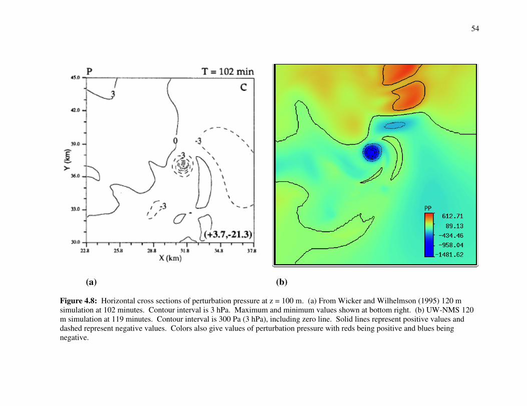
. As a result, the minimum perturbation pressure of -21 hPa in the

WW95 experiment is much lower than the -14 hPa found in this study (Figure 4.8). Lastly,

in Figure 4.9 the rotation of the vortex is again clearly seen by the wind vectors and

streamlines. The region of maximum wind speed is again found to the west of the vortex in

33

the northerly flow. The maximum wind speed of 49 m s-1

in this study surpasses that of the

WW95 experiment which gives a velocity of almost 43 m s-1

.

Both tornadoes simulated by the UW-NMS decayed in a manner similar to those in

the WW95 experiments. In both studies, low-level flow speeds up and begins to advect the

base of the vortex away from the updraft. At the same time, the rear-flank downdraft

continues to wrap around the tornado until it is completely encircled and cut off from the

updraft and low-level converging flow.

In summary, the simulation of the Wicker and Wilhelmson tornado vortex using the

UW-NMS model achieved very reasonable results. The general evolution of the supercell

thunderstorm and its tornadoes was very similar to that described in WW95. In addition,

many of the important supercell features and structures were accurately resolved and

compared well with the original WW95 experiment. However, some discrepancies between

the two experiments were found. First, the evolution of the tornadoes in the WW95

experiment occurred approximately 8 to 10 minutes before those in this study. Secondly, the

WW95 tornadoes were slightly more intense than their counterparts in all fields except

horizontal wind speed. One possible reason for the difference in intensity is that the WW95

experiments show that rain-wrapping around the tornado vortex was already being resolved

on the coarsest (600 m) grid (Figure 4.10a). Although a hook had formed in the rain field, a

fully rain-wrapped vortex was not yet observed on the coarsest grid of the UW-NMS

simulation (Figure 4.10b). However, rain-wrapping was evident on the second (120 m)

simulation. In section 4.3 a detailed discussion is given on how the intensity of a tornado

vortex may be increased through the centrifuging of rain-droplets. This process would have

a greater effect for a rain-wrapped tornado. The reason for the rain-wrapping discrepancy

34

likely lies in differing microphysics between the two studies. However, the microphysical

set-up was not provided in WW95, so this claim was not investigated.

4.1.1 Evolution of a Single Tornado Vortex at High Resolution

Up to this point the tornado vortices that have been resolved have been too weak to

produce a strong enough drop in pressure below cloud base to produce a condensation

funnel. To test the theory that a realistically strong vortex with an associated condensation

funnel can be resolved in a numerical model at sufficiently high resolution, a third grid was

added with horizontal spacing of 24 m and a domain size of 9 km by 9km. A nested vertical

grid was employed in order to increase the vertical resolution below the cloud base and more

accurately resolve the tornado. The vertical grid spacing was therefore 24 m at the surface,

stretching to 120 m at approximately 1.5 km. Above 1.5 km the vertical grid spacing is

identical to the coarser grids. The three-grid simulation ran from 115 minutes to 125

minutes, encompassing the life cycle of the second long-lived tornado in the coarser

simulation. The second and third grids moved with the lowest surface pressure, thereby

keeping tornadic activity more or less centered. The time step of the third grid was 0.2

seconds.

The evolution of the tornado vortex in the 24 m resolution simulation occurred in

much the same way as in the coarser grids. At 115 minutes, a well-defined main updraft was

present along with the downdrafts associated with the rear-flank and forward-flank gust

fronts. As time progressed, the updraft and rear-flank downdraft spiraled in toward each

other following the cyclonic rotation of the mesocyclone. Convergence of the updraft and

35

the rear-flank downdraft occurred at 122 minutes and 20 seconds, which was coincident with

the 0.95 s-1

peak in vertical vorticity near the surface (Figure 4.11a,b). The strong rotation in

the tornado vortex produced a minimum pressure of -40 hPa and wind speeds of 53 m s-1

near the surface (Figure 4.11c,d). Figure 4.12 shows the vertical extent of the tornado vortex

using the 0.2 s-1

vertical vorticity isosurface. The main portion of this vortex tube reaches to

approximately 3 km, with segments of the tube reaching as high as 12 km. Shortly after this

time, the tornado vortex weakened and dissipated as the rear-flank downdraft fully encircled

the vortex.

Despite the marked increase in intensity of the vortex at higher resolution, a

condensation funnel was not well resolved. Figure 4.13 is a vertical cross section of the log

density of cloud water condensate through the tornado vortex with a horizontal cross section

of perturbation pressure at the surface. This figure shows a slight lowering of the cloud base

coincident with the region of minimum surface pressure. However, the extent of this

lowering was only 350 m below the cloud base. This corresponds to a 35 hPa pressure drop

within the funnel. Figure 4.14 shows a close-up view of the condensation funnel at its lowest

point of descent, along with the -35 hPa isosurface of perturbation pressure. It should be

noted here that the lowest values of perturbation pressure were confined to a shallow depth

near the surface. This is likely the result of surface friction enhancing convergence at the

base of the vortex.

Pushing this experiment further, a fourth grid with horizontal resolution of 12 m and a

domain size of 3840 m by 3840 m was added. The vertical grid spacing was nested and

identical to that of the third grid. Once again, the simulation was carried out over the 10

minute period between 115 minutes and 125 minutes, encompassing the tornado life cycle.

36

The three inner grids moved with the lowest surface pressure, keeping the tornado vortex

centered in the grid box. The time step used for this experiment was 0.1 seconds.

The tornado vortex in the fourth grid peaked in intensity at 122 minutes and 40

seconds with a vertical vorticity of 1.15 s-1

. Again this was coincident with the convergence

of the updraft and intensifying rear-flank downdraft (Figure 4.15a,b). The spiraling bands of

vorticity feeding into the center of rotation are especially noticeable in Figure 4.15b. As

previously mentioned, this process concentrates the vorticity field and increases its local

density. The resultant drop in pressure at the surface was 40 hPa (Figure 4.15c). The

maximum wind speeds at the surface were 54 m s-1

(Figure 4.15d). Figure 4.16 shows a

vertical view of the tornado vortex using the 0.25 s-1

isosurface of vertical vorticity. The

height of this vortex tube reaches 4.5 km. Figure 4.17 shows a vertical cross section of the

log density of cloud water condensate taken through the tornado vortex. A noticeable

lowering below the cloud base exists, coincident with the region of minimum surface

pressure. Once again, this condensation funnel experienced only a slight descent of 300 m.

This corresponds to a 30 hPa pressure drop inside the funnel, as shown by Figure 4.18. As in

the previous experiment, the lowest pressure within the funnel is found near the surface due

to the influence of friction.

To summarize, a third and fourth grid were added to the model with horizontal

resolutions of 24 m and 12 m, respectively. The vertical resolution below cloud base was

also increased. While the tornado vortices in these high-resolution simulations were

markedly stronger than those resolved in the coarser simulations, they were not sufficient in

producing a condensation funnel that descended to the surface.

37

4.2 Effects of Vorticity Confinement

From the previous section it was shown that increasing the resolution of the model,

alone, was not sufficient in resolving a realistically strong vortex that produced a

condensation funnel. Assuming this is due to numerical diffusion weakening the strong

vorticity gradient, experiments were conducted using the VC technique in order to restore

this gradient. VC was first introduced on the third grid with 24 m resolution. A reduced time

step of 0.14 seconds was required in order for the model to sufficiently handle the faster wind

speeds that were produced. All other parameters remained unchanged and the simulation

was again run from 115 to 125 minutes.

The tornado initially developed in the same manner as discussed in previous

experiments. However with the addition of the VC term, the vortex intensified at a much

faster pace, reaching its peak at 121 minutes and 10 seconds. The low-level updraft and

downdraft at this peak time both reached a magnitude of 15 m s-1

as they converged in the

center of the mesocyclone (Figure 4.19a). The vertical vorticity reached a maximum of over

3.0 s-1

(Figure 4.19b), far exceeding that of previous experiments. This highly intensified

vortex produced a perturbation pressure near the surface of approximately -150 hPa with

horizontal wind speeds topping out at 86 m s-1

(Figure 4.19c,d). A vertical view of the

tornado vortex is given in Figure 4.20, using the 0.3 s-1

isosurface of vertical vorticity. The

vortex tube has a higher vertical extent and a lesser overall diameter than those in the

previous experiments. This shows that stretching of the vortex tube was enhanced, resulting

in its greater intensity.

38

Of particular interest is the log density of cloud water condensate in this simulation.

A lowering of the cloud base began at approximately 118 minutes with a full condensation

funnel reaching the ground at 120 minutes and 40 seconds. Figure 4.21 shows the vertical

cross section of cloud water condensate taken through the vortex tube at the peak time of the

vortex. This figure clearly shows that a condensation funnel was resolved and descended to

the surface in association with the much larger drop in pressure within the vortex. With

cloud base being approximately 1.25 km above the surface, a 125 hPa pressure drop within

the vortex would be needed for the condensation funnel to fully descend to the ground. This

was indeed achieved as shown by a close-up view of the condensation funnel with the -125

hPa isosurface of perturbation pressure extending through a large depth of the vortex in

Figure 4.22. By 122 minutes the funnel began to lift and had completely disappeared shortly

thereafter. The timing of this dissipation was again coincident with the rear-flank downdraft

encircling and weakening the vortex.

Following these results, a fourth grid was added in order to test VC at an even higher

resolution. The time step used for the fourth grid VC experiment was approximately 0.048

seconds and the fraction of maximum damping was set to 0.2 for both the horizontal and

vertical filter coefficients. All other parameters remained the same as in the experiment

without VC. The results of this experiment showed that with higher resolution, VC rapidly

spun up the vortex to such an intensity that the diameter of the vortex collapsed to a mere 36

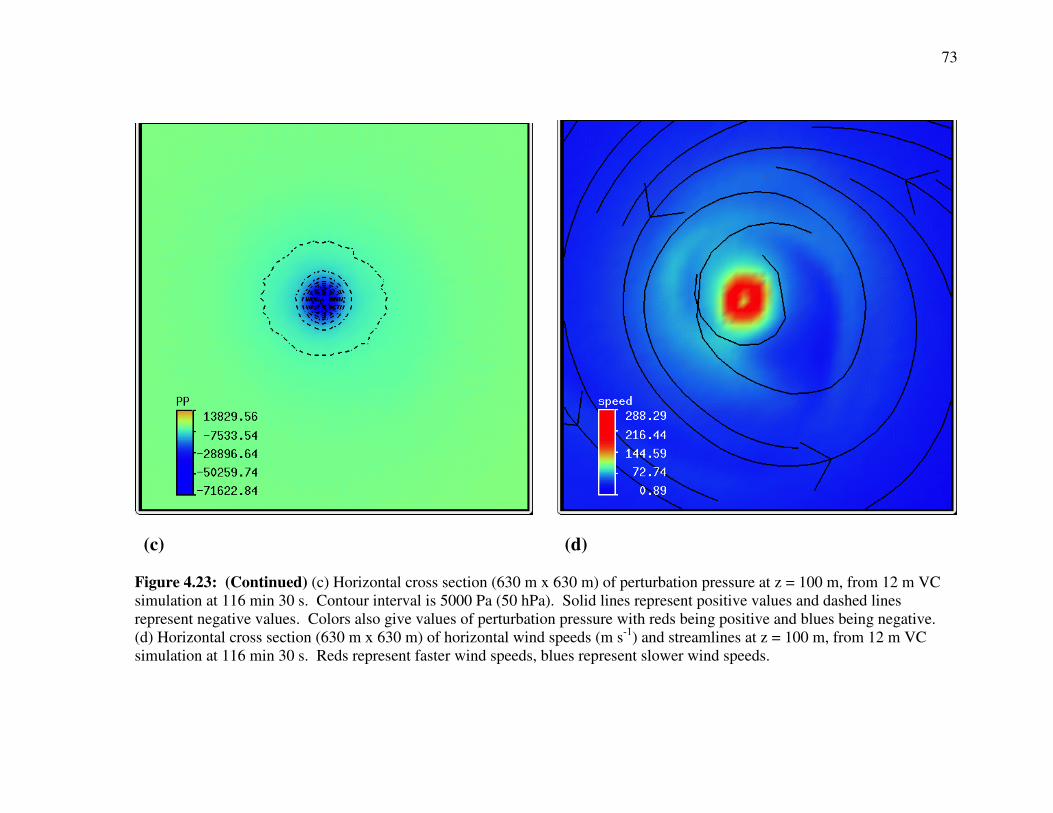
m in only 40 seconds. Figures 4.23a and 4.23b show that vertical velocities in the low-level

updraft reached 40 m s-1

, while vertical vorticity exceeded an incredible magnitude of 25 s-1

.

As a result, pressure dropped more than 500 hPa near the surface, leading to maximum wind

speeds of 220 m s-1

around the base of the vortex (Figure 4.23c,d). The 0.5 s-1

isosurface of

39

vertical vorticity shown in Figure 4.24 had already reached a height of 3.5 km. The

condensation funnel began to descend at 115 minutes and 50 seconds, reaching the surface

by 116 minutes and 20 seconds (Figure 4.25). Although a very small time step was

employed, it was likely not sufficient for the extreme wind speeds that occurred as a result of

the rapid spin-up of the vortex. The nonlinear errors that occurred in the advective scheme

forced the simulation to stop at 116 minutes and 30 seconds.

This final experiment suggests that VC does not converge to the real solution as

resolution is increased. Instead, the vortex continues to collapse to the grid scale rather than

stabilizing at a realistic tornado vortex scale. This problem must be attributed to the fact that

the VC technique lacks an energy budget such that energy is added without any constraints

on the system. In reality, the energy being used to spin up the vortex should be limited to

what is being taken from the mean flow. This is not being done in the current VC

formulation. Thus the confinement term produces a substantial change in kinetic energy but

with no physical sink of energy somewhere else in the system.

To discuss this point further, it is important to understand how energy is handled in a

numerical model. Three main scales of kinetic energy exist: kinetic energy of the mean flow

that is being predicted, kinetic energy of the sub-grid scale flow (turbulent kinetic energy),

and kinetic energy at the molecular level (thermal energy). There is also gravitational

potential energy that we can combine with thermal energy as an approximation of potential

temperature. In most numerical schemes, these scales of energy operate independently of

each other. Thus the sub-grid scale can be viewed as a reservoir for energy that is lost from a

higher scale but not yet transferred into thermal energy. Thus it is implicitly assumed that

kinetic energy lost to physical turbulence or numerical dissipation of the resolvable flow ends

40

up in this reservoir. In reality, there should exist an explicit energy budget in which energy is

exchanged between the scales (Figure 4.26). Emanuel (1996) argues that turbulent diffusion

is important and should not be neglected in tropical cyclones as it was found to indirectly

speed up the process of hurricane intensification by way of a secondary circulation that

occurs through the eyewall. In addition, Emanuel was able to determine an upper limit for

wind speeds in a mature hurricane by creating a budget in which the energy produced from

the secondary circulation was equal to dissipation in the boundary layer. When tested in two

different models, this limit proved to be a good predictor of maximum wind speeds.

Emanuel’s findings on the importance of turbulent diffusion are of particular interest

to this study because it is now hypothesized that the turbulent kinetic energy residing in the

reservoir is actually available for the spin-up of a vortex through vortex interaction. As

illustrated in Figure 4.26, turbulent kinetic energy should be accounted for by either

converting it into thermal energy through molecular dissipation or by recycling it back into

kinetic energy, perhaps through VC. The VC technique, as conceived by SU94, operates on

the principle that inertial stability blocks the cascade of energy at some level, thus prohibiting

the loss of kinetic energy to turbulent kinetic energy at the grid scale. However, this may

only be a partial explanation for the vortex growth. Thus adding to the hypothesis of SU94 is

the conjecture that turbulent kinetic energy is actually recycled back into kinetic energy

through a vortex merger process. This would divert kinetic energy from simply winding up

as thermal energy and allow for it to be refocused into strengthening the vortex. In this way,

VC would be constrained against the turbulent kinetic energy produced by dissipation of the

explicit flow. Moreover, such recycling would release the turbulent kinetic energy diverted

to thermal energy. This new theory is currently under investigation.

41

In summary, the VC technique was shown to create a realistically intense tornado

vortex in the simulation with 24 m resolution. Vertical vorticity more than doubled through

the depth of the vortex core. As a result, minimum pressure within the vortex fell at least 100

hPa lower than in the experiments performed without VC. This drop in pressure was more

than adequate for the development of a condensation funnel that descended to the surface.

However, when attempting to use VC at a higher resolution of 12 m, an unrealistically strong

vortex quickly developed. Nonlinear errors resulted in the advective scheme of the model

and therefore the simulation could not continue past 116 minutes and 30 seconds. This error

suggests that the VC technique does not converge as resolution is increased. The likely cause

of this problem is the absence of an explicit energy budget in the VC formulation. New

theories are currently being investigated to determine if a tornado vortex can be spun-up

through the recycling of energy between scales.

4.3 Effects of Centrifuging Rain Droplets

After achieving positive results with the 24 m VC simulation, tests were performed

on this third grid to determine what effect the centrifuging of rain droplets has on the strength

of a tornado vortex. To do this, experiments were conducted in which the centrifugal force

for rain droplets was turned off to see how the resultant vortex compared with the previously

run simulation. The hypothesis is that rain droplets, having no outward-directed centrifugal

force acting on them, will remain inside the funnel where a relatively higher central pressure

will result. The effect will be to weaken the intensity of the vortex.

42

In beginning this discussion it is important to note that in the absence of rotation, and

thus centrifugal force, we need only consider the terminal velocity of the rain droplets in the

vertical plane. Given the very small diameter of a rain droplet, as well as a liquid water

density 1000 times larger than that of moist air, the pressure gradient force across the droplet

becomes negligible relative to the air. As such, gravity is the only force that truly matters

when considering the vertical force balance with respect to a rain droplet. Thus, the generic

form used for the vertical terminal velocity can be given by:

b

T Agv = (4.1)

where A is a function of the microphysics, g is gravity, and b is typically set to a value of 0.5.

In the presence of rotation, and thus centrifugal force, the rain droplet experiences a terminal

velocity in all three directions, as shown by the following tendency equation for the specific

humidity of rain, qr:

DSz

vwq

y

vvq

x

vuq

t

q TwrmTvrmTurmr ++

∂

+∂+

∂

+∂+

∂

+∂−=

∂

∂ )()()( ρρρ (4.2)

where TvTu vv , and Twv are the three components of terminal velocity, ρm is the density of

moist air, S represents the source terms and D represents the dissipation terms. Therefore, we

now must consider a three-dimensional terminal velocity vector. A downward gravitational

force is exerted in the vertical and an outward centrifugal force is exerted in the horizontal on

both the air parcel and the rain droplet. However, as previously mentioned, the opposing

pressure gradient force in both the vertical and horizontal directions is much smaller for the

rain droplet in comparison to that of the air parcel. As such, it is actually the three-

dimensional pressure gradient force exerted on the air parcel and the rain droplet that

determines their respective three-dimensional terminal velocities:

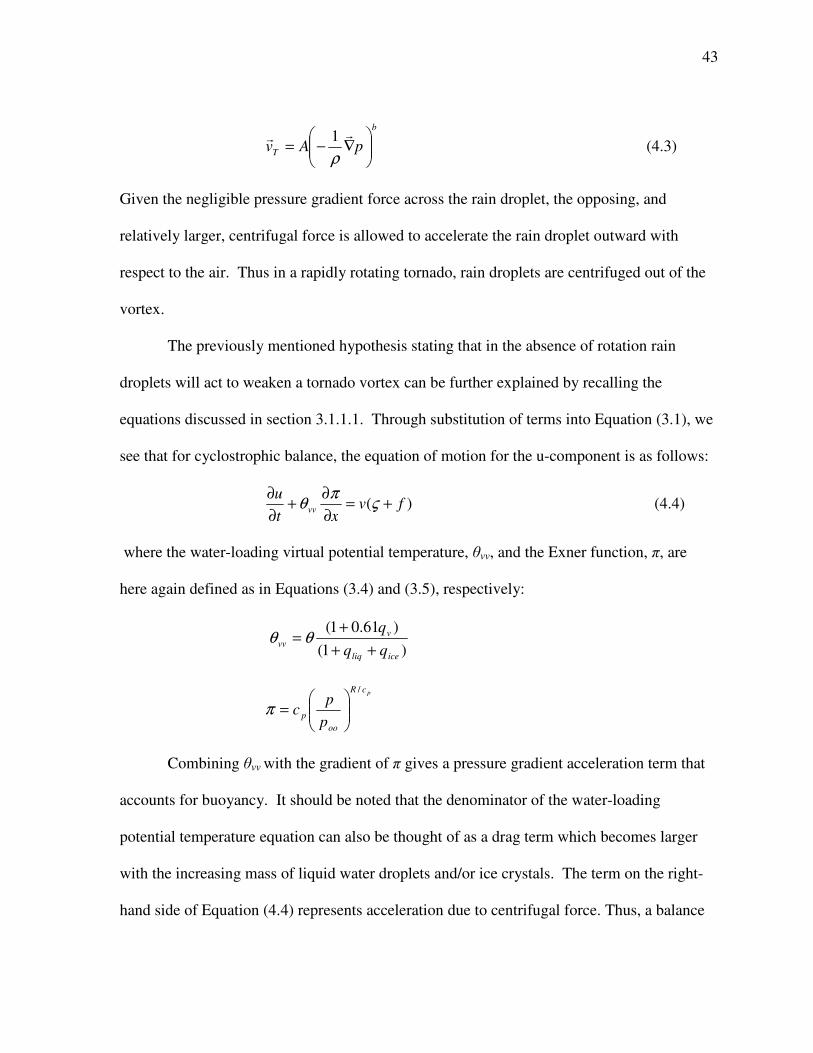
43

b

T pAv

∇−=rr

ρ

1 (4.3)

Given the negligible pressure gradient force across the rain droplet, the opposing, and

relatively larger, centrifugal force is allowed to accelerate the rain droplet outward with

respect to the air. Thus in a rapidly rotating tornado, rain droplets are centrifuged out of the

vortex.

The previously mentioned hypothesis stating that in the absence of rotation rain

droplets will act to weaken a tornado vortex can be further explained by recalling the

equations discussed in section 3.1.1.1. Through substitution of terms into Equation (3.1), we

see that for cyclostrophic balance, the equation of motion for the u-component is as follows:

)( fvxt

uvv +=

∂

∂+

∂

∂ς

πθ (4.4)

where the water-loading virtual potential temperature, θvv, and the Exner function, π, are

here again defined as in Equations (3.4) and (3.5), respectively:

)1(

)61.01(

iceliq

v

vvqq

q

++

+= θθ

pcR

oo

pp

pc

/

=π

Combining θvv with the gradient of π gives a pressure gradient acceleration term that

accounts for buoyancy. It should be noted that the denominator of the water-loading

potential temperature equation can also be thought of as a drag term which becomes larger

with the increasing mass of liquid water droplets and/or ice crystals. The term on the right-

hand side of Equation (4.4) represents acceleration due to centrifugal force. Thus, a balance

44

is achieved when the inward-directed pressure gradient acceleration equals the outward-

directed centrifugal acceleration.

When rain droplets fall into a balanced vortex, the water-loading virtual potential

temperature of the air decreases while the density of the air increases. The result is an

increase in the central pressure of the vortex and an overall decrease in the pressure gradient

acceleration. In order to bring the vortex back into balance, an adjustment takes place in

which the rain droplets are forced out of the vortex by the relatively stronger centrifugal

force, as previously discussed. As the rain droplets are being thrown out, they remove mass

from inside the vortex due to the drag force that is exerted on the surrounding air. Hence, the

central pressure of the vortex decreases, increasing the pressure gradient force and re-

strengthening the vortex.

Neglecting the centrifugal force exerted on the rain droplets as they enter a vortex

means they can no longer be thrown out in the adjustment process. Instead, the rain droplets

remain inside the vortex where they fall to the surface as their terminal velocities exceed that

of the updraft inside the tornado. As a result, the acceleration by the pressure gradient

weakens, forcing the vortex to spin down in order to achieve balance.

Figure 4.27 shows horizontal cross sections of the log density of rain through the

mid-point of the vortex (500 m above the surface) at four different times throughout the

original 24 m simulation. It is clearly seen that as time progresses from 116 minutes to 121

minutes and 10 seconds, the rain field wraps cyclonically around the vortex but is not

allowed to enter inside due to the outward directed centrifugal forces acting on the rain

droplets. Figure 4.28, on the other hand, shows that by neglecting the centrifugal force on

rain droplets, the rain is allowed to wrap into the vortex. In addition, rain droplets are

45

allowed to fall into the vortex from above. Figure 4.29a shows that initially, the vortex is

clear. Around 117 minutes the rain began to fall into the vortex and by 118 minutes (Figure

4.29b) the leading edge of the descending rain shaft had reached 1 km. A minute later

(Figure 4.29c) it is shown to be only 500 m from the surface, with the vortex completely

filled by 120 minutes.

Figures 4.30 and 4.31 compare the perturbation pressure near the surface for the

original simulation and the simulation without the centrifuging of rain droplets, respectively.

These figures show that at the intermediate times, the drop in pressure is approximately 10

hPa lower in the simulation without centrifugal force, pointing to an initially stronger vortex

than in the original simulation. However, by 121 minutes the simulation without centrifugal

force showed a minimum pressure that was 50 hPa higher than that of the original simulation.

The vertical vorticity field in Figures 4.32 and 4.33 confirms that the vorticity was initially

0.5 s-1

stronger in the simulation without centrifugal force but quickly became weaker by a

magnitude exceeding 1.0 s-1

as rain droplets filled the depth of the vortex. Analysis of the

temperature field showed that as the non-centrifuged rain began to wrap into the vortex, the

air inside became cooler due to an increase in local evaporation. By 118 minutes, the

temperature was approximately 2 K cooler than in the original vortex (Figure 4.34). This

drop in temperature within the vortex resulted in a lower pressure and therefore a slightly

stronger initial vortex in the experiments without the centrifuging of rain. However, the

majority of rain droplets entered the vortex by falling into it from above. The additional

mass inside the vortex increased the density of the air, thus leading to an increase in pressure

and a weakening of the vortex. This rise in pressure near the surface was exactly coincident

with the time the rain shaft reached the surface within the vortex.

46

With the end result being a weaker vortex in the absence of the centrifuging of rain

droplets, the vertical extent of the 0.3 s-1

vertical vorticity isosurface reached only 4.4 km

(Figure 4.35), whereas portions of the vortex reached up to 12 km in the original simulation.

In addition, the overall lesser magnitude of minimum pressure within the vortex resulted in a

condensation funnel that was 35 m from fully reaching the surface at 121 minutes and 10

seconds (Figure 4.36). The condensation funnel quickly receded and dissipated in the

following 20 seconds. Vertical distribution of minimum pressure within the vortex was also

confined to a more shallow depth when centrifugal force was neglected. Referring back to

Figure 4.22, it is evident that a very low minimum pressure extended through the entire depth

of the funnel in the original simulation. This vertical distribution acted to increase the

pressure gradient force throughout the funnel, not just near the surface. Thus, convergence

and wind speeds increased, promoting further stretching and intensification of the vortex.

In summary, by neglecting the centrifugal force on rain droplets, the simulated

tornado vortex eventually became weaker than the vortex that did centrifuge rain. Thus it

was shown that the centrifuging of hydrometeors, such as rain droplets, has the net effect of

intensifying a tornado vortex. As the hydrometeors are thrown out of the vortex, they exert a

drag force on the surrounding air, removing mass and reducing the pressure within the

vortex. The result is an increase in the pressure gradient force through a greater depth of the

funnel. Wind speeds and convergence are thus enhanced, stretching the vortex and

increasing the vertical vorticity.

47

Figure 4.1: Horizontal cross section of a tornadic supercell thunderstorm at the surface.

Thick black line represents the precipitation field as seen on radar. The solid lines with

frontal symbols represent the thunderstorm gust fronts and occlusion. The surface position of

the updrafts (UD) are finely stippled while the forward-flank downdraft (FFD) and rear-flank

downdraft (RFD) are coarsely stippled. Streamlines relative to the ground are also shown.

Location of tornado is denoted by the small encircles T in between the RFD and main UD.

(From Lemon and Doswell, 1979).

48

(a) (b)

Figure 4.2: Horizontal cross sections of vertical velocity at z = 250 m. (a) From Wicker and Wilhelmson (1995) 120 m

simulation at 87 minutes. Contour interval is 3 m s-1

. Maximum and minimum values shown at bottom right. (b) UW-NMS 120

m simulation at 96 minutes. Contour interval is 3 m s-1

, neglecting the zero line. Solid lines represent positive values and dashed

lines represent negative values. Colors also give values of vertical velocity with reds being positive and blues being negative.

49

(a) (b)

Figure 4.3: Horizontal cross sections of vertical vorticity at z = 100 m. (a) From Wicker and Wilhelmson (1995) 120 m

simulation at 87 minutes. Contour intervals are 0.01 s-1

, 0.05 s-1

, 0.1 s-1

, 0.2 s-1

, and 0.3 s-1

. Thick dark line is the 0.01 s-1

contour

representing the low-level mesocyclone. Maximum and minimum values shown at bottom right. (b) UW-NMS 120 m simulation

at 96 minutes. Contour interval is 0.04 x 105 s

-1 starting at 0.01 x 10

5 s

-1. Colors also give values of vertical vorticity with reds

being positive and blues being negative.

50

(a) (b)

Figure 4.4: Horizontal cross sections of perturbation pressure at z = 100 m. (a) From Wicker and Wilhelmson (1995) 120 m

simulation at 87 minutes. Contour interval is 3 hPa. Maximum and minimum values shown at bottom right. (b) UW-NMS 120 m

simulation at 96 minutes. Contour interval is 300 Pa (3 hPa), including zero line. Solid lines represent positive values and dashed

represent negative values. Colors also give values of perturbation pressure with reds being positive and blues being negative.

51

(a) (b)

Figure 4.5: Horizontal cross sections of horizontal winds at z = 100 m. (a) Wind vectors from Wicker and Wilhelmson (1995)

120 m simulation at 87 minutes. Maximum wind vector magnitude shown at bottom right. (b) Streamlines and wind speeds (in m

s-1

) from UW-NMS 120 m simulation at 96 minutes. Reds represent faster wind speeds and blues represent slower wind speeds.

52

(a) (b)

Figure 4.6: Horizontal cross sections of vertical velocity at z = 250 m. (a) From Wicker and Wilhelmson (1995) 120 m

simulation at 102 minutes. Contour interval is 3 m s-1

. Maximum and minimum values shown at bottom right. (b) UW-NMS 120

m simulation at 119 minutes. Contour interval is 3 m s-1

, neglecting the zero line. Solid lines represent positive values and dashed

lines represent negative values. Colors also give values of vertical velocity with reds being positive and blues being negative.

53

(a) (b)

Figure 4.7: Horizontal cross sections of vertical vorticity at z = 100 m. (a) From Wicker and Wilhelmson (1995) 120 m

simulation at 102 minutes. Contour intervals are 0.01 s-1

, 0.05 s-1

, 0.1 s-1

, 0.2 s-1

, and 0.3 s-1

. Thick dark line is the 0.01 s-1

contour

representing the low-level mesocyclone. Maximum and minimum values shown at bottom right. (b) UW-NMS 120 m simulation

at 119 minutes. Contour interval is 0.04 x 105 s

-1 starting at 0.01 x 10

5 s

-1. Colors also give values of vertical vorticity with reds

being positive and blues being negative.

54

(a) (b)

Figure 4.8: Horizontal cross sections of perturbation pressure at z = 100 m. (a) From Wicker and Wilhelmson (1995) 120 m

simulation at 102 minutes. Contour interval is 3 hPa. Maximum and minimum values shown at bottom right. (b) UW-NMS 120

m simulation at 119 minutes. Contour interval is 300 Pa (3 hPa), including zero line. Solid lines represent positive values and

dashed represent negative values. Colors also give values of perturbation pressure with reds being positive and blues being

negative.

55

(a) (b) Figure 4.9: Horizontal cross sections of horizontal winds at z = 100 m. (a) Wind vectors from Wicker and Wilhelmson (1995)

120 m simulation at 102 minutes. Maximum wind vector magnitude shown at bottom right. (b) Streamlines and wind speeds (in

m s-1

) from UW-NMS 120 m simulation at 119 minutes. Reds represent faster wind speeds and blues represent slower wind

speeds.

56

(a) (b)

Figure 4.10: Horizontal cross-sections of coarse (600 m) grid for (a) the Wicker and Wilhelmson (1995) experiment at 90

minutes and (b) the UW-NMS experiment at 98 minutes. In both figures, the heavy solid line represents the 0.25 g kg-1

rainwater

mixing ratio at 60m. The black dot in (a) indicates the region of maximum vertical vorticity, which peaks at 0.06 s-1

. Vertical

vorticity in (b) is given by the colored surface at z = 60m, where reds are positive vorticity and blues are negative vorticity.

Maximum vertical vorticity in (b) is just under 0.05 x 105 s

-1.

57

(a) (b)

Figure 4.11: (a) Horizontal cross section (4 km x 4 km) of vertical velocity at z = 250 m, from 24 m simulation at 122 min 20 s.

Contour interval is 5 m s-1

, omitting the zero line. Solid lines represent positive values and dashed lines represent negative values.

Colors also give values of vertical velocity with reds being positive and blues being negative. (b) Horizontal cross section (4 km x

4 km) of vertical vorticity at z = 100 m, from 24 m simulation at 122 min 20 s. Contour interval is 0.1 x 105 s

-1 starting at 0.05 x

105 s

-1. Colors also give values of vertical vorticity with reds being positive and blues being negative.

58

(c) (d)

Figure 4.11: (Continued) (c) Horizontal cross section (4 km x 4 km) of perturbation pressure at z = 100 m, from 24 m simulation

at 122 min 20 s. Contour interval is 300 Pa (3 hPa), including zero line. Solid lines represent positive values and dashed lines

represent negative values. Colors also give values of perturbation pressure with reds being positive and blues being negative. (d)

Horizontal cross section (4 km x 4 km) of horizontal wind speeds (in m s-1

) and streamlines at z = 100 m, from 24 m simulation at

122 min 20 s. Reds represent faster wind speeds, blues represent slower wind speeds.

59

Figure 4.12: Vertical view of 0.2 s-1

vertical vorticity isosurface with colored horizontal

cross section of perturbation pressure (Pa) and horizontal streamlines at the surface. From 24

m simulation at 122 min 20 s.

60

Figure 4.13: Vertical cross section of the log density of cloud water condensate (gray

contours) with colored horizontal cross section of perturbation pressure (Pa) at the surface.

From 24 m simulation at 122 min 20 s. Contour interval in the cloud is 0.5.

61

Figure 4.14: Close-up vertical cross section of the log density of cloud water condensate

with -3500 Pa (-35 hPa) perturbation pressure isosurface (blue). Colored surface is

horizontal cross section of perturbation pressure (Pa). From 24 m simulation at 122 min 30 s.

62

(a) (b)

Figure 4.15: (a) Horizontal cross section of vertical velocity at z = 250 m, from 12 m simulation at 122 min 40 s. Contour

interval is 5 m s-1

, omitting the zero line. Solid lines represent positive values and dashed lines represent negative values. Colors

also give values of vertical velocity with reds being positive and blues being negative. (b) Horizontal cross section of vertical

vorticity at z = 100 m, from 12 m simulation at 122 min 40 s. Contour interval is 0.1 x 105 s

-1 starting at 0.05 x 10

5 s

-1. Colors

also give values of vertical vorticity with reds being positive and blues being negative.

63

(c) (d)

Figure 4.15: (Continued) (c) Horizontal cross section of perturbation pressure at z = 100 m, from 12 m simulation at 122 min 40

s. Contour interval is 300 Pa (3 hPa), including zero line. Solid lines represent positive values and dashed lines represent negative

values. Colors also give values of perturbation pressure with reds being positive and blues being negative. (d) Horizontal cross

section of horizontal wind speeds (in m s-1

) and streamlines at z = 100 m, from 12 m simulation at 122 min 40 s. Reds represent

faster wind speeds, blues represent slower wind speeds.

64

Figure 4.16: Vertical view of 0.25 s-1

vertical vorticity isosurface with colored horizontal

cross section of perturbation pressure (Pa) and horizontal streamlines at the surface. From 12

m simulation at 122 min 40 s.

65

Figure 4.17: Vertical cross section of the log density of cloud water condensate (gray

contours) with colored horizontal cross section of perturbation pressure at the surface (Pa).

From 12 m simulation at 122 min 40 s. Contour interval in the cloud is 0.5.

66

Figure 4.18: Close-up vertical cross-section of the log density of cloud water condensate

with -3000 Pa (-30 hPa) perturbation pressure isosurface (blue). Colored surface is

horizontal cross section of perturbation pressure (Pa). From 12 m simulation at 122 min 40 s.

67

(a) (b)

Figure 4.19: (a) Horizontal cross section (2 km x 2 km) of vertical velocity at z = 250 m, from 24 m VC simulation at 121 min

10 s. Contour interval is 5 m s-1

, omitting the zero line. Solid lines represent positive values and dashed lines represent negative

values. Colors also give values of vertical velocity with reds being positive and blues being negative. (b) Horizontal cross

section (2 km x 2 km) of vertical vorticity at z = 100 m, from 24 m VC simulation at 121 min 10 s. Contour interval is 0.1 x 105

s-1

starting at 0.05 x 105 s

-1. Colors also give values of vertical vorticity with reds being positive and blues being negative.

68

(c) (d)

Figure 4.19: (Continued) (c) Horizontal cross section (2 km x 2 km) of perturbation pressure at z = 100 m, from 24 m VC

simulation at 121 min 10 s. Contour interval is 1000 Pa (10 hPa). Solid lines represent positive values and dashed lines

represent negative values. Colors also give values of perturbation pressure with reds being positive and blues being negative.

(d) Horizontal cross section (2 km x 2 km) of horizontal wind speeds (in m s-1

) and streamlines at z = 100 m, from 24 m VC

simulation at 121 min 10 s. Reds represent faster wind speeds, blues represent slower wind speeds.

69

Figure 4.20: Vertical view of 0.30 s-1

vertical vorticity isosurface with colored horizontal

cross section of perturbation pressure (Pa) and horizontal streamlines at the surface. From 24

m VC simulation at 121 min 10 s.

70

Figure 4.21: Vertical cross section of the log density of cloud water condensate (gray

contours) with colored horizontal cross section of perturbation pressure (Pa) at the surface.

From 24 m VC simulation at 121 min 10 s. Contour interval in the cloud is 0.5.

71

Figure 4.22: Close-up vertical cross section of the log density of cloud water condensate

with -12500 Pa (-125 hPa) perturbation pressure isosurface (blue). Colored surface is

horizontal cross section of perturbation pressure (Pa). From 24 m VC simulation at 121 min

10 s.

72

Figure 4.23: (a) Horizontal cross section (630 m x 630 m) of vertical velocity at z = 250 m, from 12 m VC simulation at 116

min 30 s. Contour interval is 5 m s-1

, omitting the zero line. Solid lines represent positive values and dashed lines represent

negative values. Colors also give values of vertical velocity with reds being positive and blues being negative. (b) Horizontal

cross section (630 m x 630 m) of vertical vorticity at z = 100 m, from 12 m VC simulation at 116 min 30 s. Contour interval is

5.0 x 105 s

-1 starting at 0.5 x 10

5 s

-1. Colors also give values of vertical vorticity with reds being positive and blues being

negative.

73

(c) (d)

Figure 4.23: (Continued) (c) Horizontal cross section (630 m x 630 m) of perturbation pressure at z = 100 m, from 12 m VC

simulation at 116 min 30 s. Contour interval is 5000 Pa (50 hPa). Solid lines represent positive values and dashed lines

represent negative values. Colors also give values of perturbation pressure with reds being positive and blues being negative.

(d) Horizontal cross section (630 m x 630 m) of horizontal wind speeds (m s-1

) and streamlines at z = 100 m, from 12 m VC

simulation at 116 min 30 s. Reds represent faster wind speeds, blues represent slower wind speeds.

74

Figure 4.24: Vertical view of 0.50 s-1

vertical vorticity isosurface with colored horizontal

cross section of perturbation pressure (Pa) and horizontal streamlines at the surface. From 12

m VC simulation at 116 min 30 s.

75

Figure 4.25: Vertical cross section of the log density of cloud water condensate (gray

contours) with colored horizontal cross section of perturbation pressure (Pa) at the surface.

From 12 m VC simulation at 116 min 30 s. Contour interval in the cloud is 0.5.

76

Figure 4.26: Flow diagram illustrating an explicit budget of energy, coupling kinetic energy

(KE), turbulent kinetic energy (TKE) and the combination of thermal energy and potential

energy (PE), which is simply potential temperature, θ. Energy can now be exchanged

between the different scales. Physical turbulence and numerical dissipation convert KE into

TKE, while molecular dissipation converts TKE into potential temperature. Buoyancy

production can then convert potential temperature back into TKE, while TKE can be recycled

back into KE through a vortex merger process.

KE 1/2(u

2+v

2+w

2)

TKE 1/2(u’’

2+v’’

2+w’’

2)

Thermal Energy

CpT

Numerical Dissipation Physical Turbulence

Molecular Dissipation

Vortex Merger

(Recycling)

Buoyancy

Production

PE gz

77

Figure 4.27: Horizontal cross sections of the log density of rain (LDNRR) at z = 500 m

from 24 m VC simulation at (a) 116 minutes, (b) 118 minutes, (c) 119 minutes and (d) 121

minutes and 10 seconds.

78

Figure 4.28: Same as Figure 4.22 except without centrifugal force.

79

Figure 4.29: Vertical cross sections of the log density of rain (LDNRR) taken through the

tornado vortex. From 24 m VC simulation without centrifugal force at (a) 116 minutes, (b)

118 minutes, (c) 119 minutes and (d) 121 minutes and 10 seconds. Arrows point to

leading edge of rain shaft descending through center of vortex.

80

Figure 4.30: Horizontal cross sections (2.8 km x 2.8 km) of perturbation pressure at z =

100 m from 24 m VC simulation at (a) 116 minutes, (b) 118 minutes, (c) 119 minutes and

(d) 121 minutes and 10 seconds. Contour interval is 1000 Pa (10 hPa).

81

Figure 4.31: Same as Figure 4.24 except without centrifugal force.

82

Figure 4.32: Horizontal cross sections (2.8 km x 2.8 km) of vertical vorticity at z = 100 m

from 24 m VC simulation at (a) 116 minutes, (b) 118 minutes, (c) 119 minutes and (d) 121

minutes and 10 seconds. Contour interval is 0.5 x 105 s

-1 starting at 0.05 x 10

5 s

-1.

83

Figure 4.33: Same as Figure 4.27 except without centrifugal force.

84

(a) (b)

Figure 4.34: Horizontal cross section of temperature within the tornado vortex at z = 500

m. From 24 m VC simulation (a) with and (b) without the centrifuging of rain droplets.

Contour interval is 2 K.

85

Figure 4.35: Vertical view of 0.30 s-1

vertical vorticity isosurface with colored horizontal

cross section of perturbation pressure (Pa) and horizontal streamlines at the surface. From 24

m VC simulation without centrifugal force at 121 min 10 s.

86

Figure 4.36: Vertical cross section of the log density of cloud water condensate (gray

contours) with colored horizontal cross section of perturbation pressure (Pa). From 24 m

VC simulation without centrifugal force at 121 min 10 s. Contour interval in the cloud is

0.5.

87

Chapter 5

Conclusion

Numerical modeling of small-scale atmospheric flow has made marked advancements

in recent years. Despite this fact, resolving a realistically strong tornado vortex and

associated condensation funnel has proven difficult. This research set forth to examine the

theories behind this problem and to study the effects of one possible solution, the Vorticity

Confinement (VC) technique. Experiments were performed using the University of

Wisconsin - Nonhydrostatic Modeling System (UW-NMS) and modeled after the Wicker and

Wilhelmson (1995) idealized tornadic supercell. The WW95 experiments were first

extended by simulating the development of a single tornado vortex at resolutions of 24 m and

12 m. These high-resolution simulations accurately resolved many small-scale features of

the tornado life cycle, but failed to produce a vortex strong enough to develop a condensation

funnel. Therefore it was proven that by simply increasing the model resolution, a

realistically strong vortex could not be achieved even when using sophisticated schemes in

which kinetic energy and enstrophy are conserved.

Employing the VC technique on the simulation with 24 m resolution, led to very

positive results in which a realistically intense tornado vortex developed. The associated

minimum pressure within the vortex was low enough that a condensation funnel developed

and descended to the surface. Despite this success, extending VC to a higher resolution grid

proved to be disappointing. The simulation with 12 m resolution resulted in an

unrealistically strong and narrow vortex that developed in less than a minute. This incredibly

fast intensification resulted in nonlinear errors in the advective scheme, forcing the

88

simulation to stop after only 90 seconds. In light of these results, it is concluded that

although the VC technique succeeds in producing a beautiful and realistic condensation

funnel, it does not converge to the real solution as resolution is increased. The problem is

attributed to the absence of an explicit energy budget to physically constrain the energy

added to the system by the confinement term. Despite being physically flawed, the VC

technique does provide hope in finding the missing mechanism needed to resolve strong

vortices. New theories are currently being investigated in which an explicit energy budget is

imposed on the system, allowing for the exchange of energy between scales. In this system,

kinetic energy from the mean flow is converted into turbulent kinetic energy. The vortex is

can then be strengthened through the recycling of turbulent kinetic energy back into kinetic

energy. The original VC technique artificially strengthens the vortex by assuming that

inertial stability blocks the loss of kinetic energy to turbulent kinetic energy.

Final experiments were performed in which the centrifugal force exerted on rain

droplets in a vortex was neglected. Allowing rain droplets to fall into the vortex core without

being centrifuged outward, resulted in an increase of pressure within the vortex. This rise in

pressure weakened the inward-directed pressure gradient force, thus decreasing the strength

of the tornado vortex. From these results it is concluded that the centrifuging of

hydrometeors, such as rain droplets, can intensify the strength of a vortex by removing mass

and reducing the minimum pressure inside the vortex. This strengthening of the pressure

gradient force leads to faster wind speeds and stronger convergence, thus intensifying the

vorticity of the tornado.

89

Appendix

The Bernoulli form of momentum acceleration is a function of the three components

of the two-dimensional potential vorticity (i

η ) and a three-dimensional, invariant kinetic

energy (k) field. Using this form allows the final three-dimensional momentum acceleration

to be finite-differenced in a way that preserves the conservation of the two-dimensional

potential vorticity and kinetic energy fields against numerical biases. In addition, finite-

differencing can take place in which there is a minimization or removal of artificial

numerical sources of mean potential enstrophy, a common issue when finite-differencing the

momentum equations. Arakawa and Lamb (1981, hereafter referred to as AL81) and

Sadourny (1976) both made use of these advantages for a quasi-two-dimensional hydrostatic

system. The following discussion details how this finite differencing scheme was modified

for a fully coupled three-dimensional flow on an Arakawa C-grid.

The finite-differenced form of the two-dimensional potential vorticity used in the

original AL81 scheme is given by:

( ) ( )

( )

1 , 1, , 1/ 2, 1

1/ 2

1/ 2, , 1

, , , 1/ 2,

3 3 2 2, 1/ 2, 1/ 2

1 , 1/ 2, 1/ 2

32

1/ 2, ,

1 1 31/ 2, , 1/ 2

2 1/ 2, , 1/ 2

3

cos cos1 (A1)

cos

1

j i j k j i j k

j

i j k

i j k i j k

i j k

i j kz

y

i j k

i j k

i j kz

x

u u u u

xx

u u u

x

φ φη

φρ

η

ρ

+ + + +

+

+ +

+

+ +

+ +

+

+ +

+ +

− − = − ∆∆

−= −

∆

( )

( ) ( )

1, ,

1, 1/ 2, 1 1/ 2. 1,

1/ 2 1/ 2

, ,

3

1

, 1/ 2, 1/ 2, ,

2 2 1 11/ 2, 1/ 2,

3 1/ 2, 1/ 2,

1 2

(A2)cos

cos cos1 (A3)

cos cos

i j k

j

i j k j i j k j

j j

i j k

i j k i j k

i j k

i j ky

x

u

x

u u u u

x x

φ

φ φη

φ φρ

+

+ + + + +

+ +

+ +

+ +

+ +

− ∆

− − = − ∆ ∆

90

The i, j, and k superscripts refer to the ( )1 2 3, ,x x x grid number on a three-dimensional

Arakawa C-grid where velocity and scalar time-dependent variables are located at

( )1/ 2, , , 1/ 2, , , 1/ 2 , ,

1 2 3, , ,i j k i j k i j k i j ku u u T+ + + . Latitude, jφ , is only a function of 2x in the rotated

spherical grid. It should be pointed out that curvature terms are implicit to this system

through the use of the cosine function for the 2x differencing in the 1 3 and η η equations.

Despite maintaining the conservation of specific kinetic energy (k) in several different

forms, problems arise when using the finite difference form of k, as detailed by AL81. These

difficulties are the result of calculating the gradient of kinetic energy with different velocity

points than those used for the calculation of vorticity-based accelerations. This ultimately

leads to an inaccurate computation of the momentum acceleration terms, thus destroying the

solution. To correct the problem, the kinetic energy and two-dimensional potential vorticity

are averaged so that the same velocity points are used in the calculations of the kinetic energy

gradient and the vorticity acceleration terms.

The specially averaged finite difference form of the kinetic energy is given by:

( ), ,

3, ,

, ,

1

1 2

2 3

nm

l l

i j kx

xi j k x x

i j k

l l

l

k u u e=

= + ∑ (A4)

where the subscript m n l≠ ≠ , and , ,i j ke is the turbulent kinetic energy which is predicted or

diagnosed from the physical turbulence model. The averages of the two-dimensional

potential vorticity are weighted by density, as shown in the following equations:

91

( )

( )

11

23

1

23

22

13

2

13

, 1/ 2, 1/ 2

, 1/ 2, 1/ 2

1

, 1/ 2, 1/ 2

1 , 1/ 2, 1/ 2

1/ 2, , 1/ 2

1/ 2, , 1/ 2

2

1/ 2, , 1/ 2

2 1/ 2, , 1/

(A5)

xx

i j kx

x i j k

i j kx

i j kx

x

xx

i j kx

x i j k

i j kx

i j kx

x

ρ η

η

ρ

ρ η

η

ρ

+ ++ +

+ +

+ +

+ ++ +

+ +

+ +

=

=

( )

33

21

3

21

2

1/ 2, 1/ 2,

1/ 2, 1/ 2,

3

1/ 2, 1/ 2,

3 1/ 2, 1/ 2,

(A6)

(A7)

xx

i j kx

x i j k

i j kx

i j kx

x

ρ η

η

ρ

+ ++ +

+ +

+ +

=

The above averages are normal to the two-dimensional plane of the finite-differenced,

enstrophy-conserving AL81 formulation. Therefore, they invoke no change to the original

scheme.

As defined by AL81, the momentum terms are as follows:

1

2

1/ 2, , 1/ 2, ,

1 1 1

, 1/ 2, , 1/ 2,

2 2 2

, , 1/ 2 , , 1/ 2

3 2

1cos (A8)

2

1 (A9)

2

1

2

xi j k i j k j

xi j k i j k

xi j k i j k

m u x

m u x

m u

ρ φ

ρ

ρ

+ +

+ +

+ +

= ∆

= ∆

= 3

3 (A10)x∆

As seen by these equations, each of the three momentum components is weighted by the grid

spacing used in the same component direction. The spherical effect, as seen by the cosine

function, was accounted for in the AL81 formulation. However, variable grid spacing was

not. For the purposes of the NMS model, variable grid spacing only comes into play in the

vertical direction.

92

The enstrophy-conserving, finite difference form of the momentum equations give us

the full, three-dimensional inertial terms for momentum:

( ) ( ) ( ) ( )( )

( ) ( ) ( ) ( )( )

1/ 2, , 1/ 2, , 1, , , ,1/ 2, ,

1 2 3 3 2

1

, 1/ 2, , 1/ 2, , 1, , ,, 1/ 2,

2 3 1 1 3

2

, , 1/ 2

3

1 (A11)

cos

1 (A12)

1

i j k i j k i j k i j ki j k

j

i j k i j k i j k i j ki j k

i j k

I m m k kx

I m m k kx

Ix

η ηφ

η η

+ + ++

+ + ++

+

= − − − ∆

= − − − ∆

=∆

( ) ( ) ( ) ( )( )1/ 2, , 1/ 2, , , , 1 , ,

1 2 2 1

3

(A13)i j k i j k i j k i j k

m m k kη η+ + + − − −

The nine vorticity terms, ( )i jmη , in Equations (A11)-(A13) are fully defined in AL81.

For the conciseness of this discussion, only those terms found in the 1u equation of motion

are defined here:

( )1/ 2, , 1, 1/ 2, 1/ 2, 1/ 2, , 1/ 2, 1/ 2, 1/ 2,

2 3 2 23 2 23

1, 1/ 2, 1/ 2, 1/ 2, 1, 1/ 2, 1/ 2, 1/ 2,

2 23 2 23

1/ 2, , 3/ 2, , 1/ 2, , 1/ 2, ,

23 1 23 1

(A14)

i j k i j k i j k i j k i j k

i j k i j k i j k i j k

i j k i j k i j k i j k

m m m

m m

u u

m

η α β

γ δ

ε ϕ

+ + + + + + + +

+ − + + + − + +

+ + − −

= + +

+ +

− +

( )1/ 2, , 1, , 1/ 2 1/ 2, , 1/ 2 , 1/ 2, 1/ 2, , 1/ 2

3 2 3 32 3 32

1, , 1/ 2 1/ 2, , 1/ 2 1, , 1/ 2 1/ 2, , 1/ 2

3 32 3 32

1/ 2, , 3/ 2, , 1/ 2, , 1/ 2, ,

32 1 32 1

(A15)

i j k i j k i j k i j k i j k

i j k i j k i j k i j k

i j k i j k i j k i j k

m m

m m

u u

η α β

γ δ

ε ϕ

+ + + + + + + +

+ − + + + − + +

+ + − −

= + +

+ +

− +

where , , , , , and ij ij ij ij ij ij

α β γ δ ε ϕ are the weighting coefficients defined by AL81, which

have been extended for this three-dimensional formulation. Again, for the conciseness of

this discussion, only the weighting coefficients pertaining to the ( )1/ 2, ,

2 3

i j km η

+ terms in the 1u

equation are defined here:

93

3 3 3

3 3 3

1/ 2, 1/ 2, 1/ 2, 1/ 2, 3/ 2, 1/ 2, 1/ 2, 1/ 2, 1/ 2, 1/ 2,

23 3 3 3 23

1/ 2, 1/ 2, 1/ 2, 1/ 2, 1/ 2, 1/ 2, 1/ 2, 1/ 2,

23 3 3 3

12 (A16)

24

12

24

x x xi j k i j k i j k i j k i j k

x x xi j k i j k i j k i j k

a

b

α η η η

β η η η

+ + + + + + + − + +

+ + + + − + + −

= + + +

= + + +

3 3 3

3

1/ 2, 1/ 2,

23

1/ 2, 1/ 2, 1/ 2, 1/ 2, 1/ 2, 1/ 2, 1/ 2, 3/ 2, 1/ 2, 1/ 2,

23 3 3 3 23

1/ 2, 1/ 2, 1/ 2, 1/ 2, 3/ 2

23 3 3

(A17)

12 (A18)

24

12

24

i j k

x x xi j k i j k i j k i j k i j k

xi j k i j k i

gγ η η η

δ η η

+ +

+ + + + − + + + + +

+ + + + +

= + + +

= +

( )

3 3, 1/ 2, 1/ 2, 3/ 2, 1/ 2, 1/ 2,

3 23

1/ 2, 1/ 2, 1/ 2, 1/ 2, 1/ 2, 1/ 2,

23 23 23

23

(A19)

1 (A20)

24

x xj k i j k i j k

i j k i j k i j k

i

d

d a

η

ε

ϕ

+ + + + +

+ + + − + +

+

+ +

= −

( )

3 3

1/ 2, 1/ 2, 1/ 2, 1/ 2, 1/ 2, 1/ 2,

23 23

1/ 2, 1/ 2, 3/ 2, 1/ 2, 1/ 2, 1/ 2,

23 3 3

1 (A21)

24

where,

j k i j k i j k

x xi j k i j k i j k

g b

a η η

+ + + + +

+ + + − + +

= −

= −

3 31/ 2, 1/ 2, 1/ 2, 1/ 2, 1/ 2, 1/ 2,

23 3 3

1/ 2, 1/ 2 3/ 2,

23 3

(A22)

(A23)x x

i j k i j k i j k

j k i j

b

d

η η

η

+ + − − + +

+ + + +

= −

=3 3

3 3

3/ 2, 1/ 2, 1/ 2, 3/ 2, 3/ 2,

3 23

1/ 2, 1/ 2, 1/ 2, 3/ 2, 1/ 2, 1/ 2, 1/ 2, 3/ 2,

23 3 3 23

(A24)

x xk i j k i j k

x xi j k i j k i j k i j k

b

g a

η

η η

+ + + +

+ + − + + + − +

− = −

= − = − (A25)

94

References

Arakawa, A., 1966: Computational design for long-term numerical integration of the

equations of fluid motions: Two dimensional incompressible flow. J. Comput. Phys.,

1, 119-143.

Arakawa, A., and V. R. Lamb, 1981: A potential enstrophy and energy conserving scheme

for the shallow water equations. Mon. Wea. Rev., 109, 18-36.

Bluestein, H. B., J. G. LaDue, H. Stein, D. Speheger, and W. P. Unruh, 1993: Doppler radar

wind spectra of supercell tornadoes. Mon. Wea. Rev., 121, 2200-2221.

Brown, R. A., D. W. Burgess, and K. C. Crawford, 1973: Twin tornado cyclones within a

severe thunderstorm. Weatherwise, 26, 63-71.

Burgess, D. B., M. A. Magsig, J. Wurman, D. C. Dowell, and Y. Richardson, 2002: Radar

observations of the 3 May 1999 Oklahoma City tornado. Wea. Forecasting, 17, 456-

471.

Clark, T. L., 1977: A small scale dynamic model using a terrain-following coordinate

transformation. J. Comp. Phys., 24, 186-215.

95

Davies-Jones, R. P., D. W. Burgess, and M. P. Foster, 1990: Test of helicity as a forecast

parameter. Preprints, 16th

Conf. on Severe Local Storms, Kananaskis Park, AB,

Canada, Amer. Meteor. Soc., 588-592.

Dowell, D. C., C. R. Alexander, J. M. Wurman, and L. J. Wicker, 2005: Centrifuging of

hydrometeors and debris in tornadoes: Radar-reflectivity patterns and wind-

measurement errors. Mon. Wea. Rev., 133, 1501-1524.

Dowell, D. C., and H. B. Bluestein, 2002: The 8 June 1995 McLean, Texas, storm. Part I:

Observations of cyclic tornadogenesis. Mon. Wea. Rev., 130, 2626-2648.

Emanuel, K. A., 1997: Some aspects of hurricane inner-core dynamics and energetics. J.

Atmos. Sci., 54, 1014–1026.

Fedkiw, R., J. Stam, and H. W. Jensen, 2001: Visual Simulation of Smoke. Proceedings of

SIGGRAPH 2001, Los Angeles, CA, 23-30.

Fan, M., Y. Wenren, W. Dietz, M. Xiao, and J. Steinhoff, 2002: Computing blunt body

flows on coarse grids using vorticity confinement. J. Fluids Eng., 124, No. 4.

Grasso, L. D., and W. R. Cotton, 1995: Numerical simulation of a tornado vortex. J. Atmos.

Sci., 52, 1192-1203.

96

Kangieser, P. C., 1954: A physical explanation of the hollow structure of waterspout tubes.

Mon. Wea. Rev., 82, 147-152.

Klemp, J. B., and R. Rotunno, 1983: A study of the tornadic region within a supercell

thunderstorm. J. Atmos. Sci., 40, 359-377.

Klemp, J. B., and R. B. Wilhelmson, 1978a: The simulation of three-dimensional convective

storm dynamics. J. Atmos. Sci., 35, 1070-1096.

Klemp, J. B., and R. B. Wilhelmson, 1978b: Simulations of right- and left-moving storms

produced through storm splitting. J. Atmos. Sci., 35, 1097-1110.

Klemp, J. B., R. B. Wilhelmson, and P. S. Ray, 1981: Observed and numerically simulated

structure of a mature supercell thunderstorm. J. Atmos. Sci., 38, 1558-1580.

Lemon, L. R., and C. A. Doswell III, 1979: Severe thunderstorm evolution and mesocyclone

structure as related to tornadogenesis. Mon. Wea. Rev., 107, 1184-1197.

Lilly, D. K., 1986: The structure, energetics and propagation of rotating convective storms.

Part I: Energy exchange with the mean flow. J. Atmos. Sci., 43, 113-125.

Louis, J. F., 1979: A parametric model of vertical eddy fluxes in the atmosphere. Bound.-

Layer Meteor., 17, 187-202.

97

Miyazaki, R., Y. Dobashi, and T. Nishita, 2002: Simulation of cumuliform clouds based on

computational fluid dynamics. Short presentations, The Eurographics Association.

Redelsperger, J. L., and G. Someria, 1982: Methode de representation de la turbulence

associe aux precipitations dans un modele tri-dimensionnel de convection nuageuses.

Bound.-Layer Meteor., 24, 231-252.

Schlesinger, R. E., 1978: A three-dimensional numerical model of an isolated thunderstorm.

Part I: Comparative experiments for variable ambient wind shear. J. Atmos. Sci., 35,

690-713.

Schlesinger, R. E., 1980: A three-dimensional numerical model of an isolated thunderstorm.

Part II: Dynamics of updraft splitting and mesovortex couplet evolution. J. Atmos.

Sci., 37, 395-420.

Smolarkiewicz and Margolin, 1993: On forward-in-time differencing for fluids: Extension to

a curvilinear framework. Mon. Wea. Rev., 121, 1847–1859

Steinhoff, J., and D. Underhill, 1994: Modification of the Euler equations for “vorticity

confinement”: Application to the computation of interacting vortex rings. Phys.

Fluids, 6, 2738-2744.

98

Tripoli, G. J., and W. R. Cotton, 1986: An intense quasi-steady thunderstorm over

mountainous terrain. Part IV: Three-dimensional numerical simulation. J. Atmos.

Sci., 43, 894-912.

Tripoli, G. J., 1992a: A nonhydrostatic mesoscale model designed to simulate scale

interaction. Mon. Wea. Rev., 120, 1342-1359.

Tripoli, G. J., 1992b: An explicit three-dimensional nonhydrostatic numerical simulation of

a tropical cyclone. Meteor. Atmos. Phys., 49, 229-254.

Tripoli, G. J., C. Medaglia, A. Mugnai, and E. A. Smith, 2004: Numerical simulation of

waterspouts observed in the Tyrrhenian Sea. Preprints, 11th

conf. on mesoscale

processes, Albuquerque, NM, Amer. Meteor. Soc.

Tripoli, G. J., and E. A. Smith, 2007: Scalable nonhydrostatic regional-mesoscale-cloud

model featuring variable-stepped topography coordinates: Formulation and

performance on classic obstacle flow patterns. Submitted to Mon. Wea. Rev.

Wakimoto, R. M., B. E. Martner, 1992: Observations of a Colorado tornado. Part II:

Combined photogrammetric and Doppler radar analysis. Mon. Wea. Rev. 120, 522-

543.

99

Weisman, M. L., and J. B. Klemp, 1982: The dependence of numerically simulated

convective storms on vertical wind shear and buoyancy. Mon. Wea. Rev., 110, 504-

520.

Weisman, M. L., and J. B. Klemp, 1984: The structure and classification of numerically

simulated convective storms in directionally varying wind shears. Mon. Wea. Rev.,

112, 2479-2498.

Weisman, M. L., C. Davis, and J. Done, 2005: The promise and challenge of explicit

convective forecasting with the WRF model. Preprints, 2004 MM5 Users’ Workshop,

Boulder Colorado, NCAR.

Wicker, L. J., D. W. Burgess, and H. Bluestein, 1984: The prestorm environment of the

severe weather outbreak in western Oklahoma on 22 May 1981. Preprints, 13th

Conf.

on Severe Local Storms, Tulsa, OK, Amer. Meteor. Soc., 281-282.

Wicker, L. J., and R. B. Wilhelmson, 1995: Simulation and analysis of tornado development

and decay within a three-dimensional supercell thunderstorm. J. Atmos. Sci., 52,

2675-2703.

Wilhelmson, R. B., and J. B. Klemp, 1978: A numerical study of storm splitting that leads to

long-lived storms. J. Atmos. Sci., 35, 1974-1986.

100

Wilhelmson, R. B., and J. B. Klemp, 1981: A three-dimensional numerical simulation of

splitting severe storms on 3 April 1964. J. Atmos. Sci., 38, 1581-1600.

Wurman, J., J. M. Straka, and E. N. Rasmussen, 1996: Fine-scale Doppler radar

observations of tornadoes. Science, 272, 1774-1777.

Wurman, J., and S. Gill, 2000: Fine-scale radar observations of the Dimmitt, Texas (2 June

1995) tornado. Mon. Wea. Rev., 128, 2135-2164.

Xue, M., 2004: Tornadogenesis within a simulated supercell storm. Preprints, 22nd Conf. on

Severe Local Storms, Hyannis, MA, Amer. Meteor. Soc.