Numerical Linear Algebra - EconStor · 2020-01-16 · Numerical Linear Algebra 3 Theorem 1. Let...

Numerical Linear Algebra

Lenka Cızkova1 and Pavel Cızek2

1 Faculty of Nuclear Sciences and Physical Engineering, Czech TechnicalUniversity in Prague, Brehova 7, 115 19 Praha 1, The Czech Republiclenka [email protected]

2 Tilburg University, Department of Econometrics & Operations ResearchRoom B 516, P.O. Box 90153, 5000 LE Tilburg, The [email protected]

Many methods of computational statistics lead to matrix-algebra or numeric-al-mathematics problems. For example, the least squares method in linearregression reduces to solving a system of linear equations, see Chapter ??. Theprincipal components method is based on finding eigenvalues and eigenvectorsof a matrix, see Chapter ??. Nonlinear optimization methods such as Newton’smethod often employ the inversion of a Hessian matrix. In all these cases, weneed numerical linear algebra.

Usually, one has a data matrix X of (explanatory) variables, and inthe case of regression, a data vector y for dependent variable. Then thematrix defining a system of equations, being inverted or decomposed typi-cally corresponds to X or X�X. We refer to the matrix being analyzed asA = {Aij}m,n

i=1,j=1 ∈ Rm×n and to its columns as Ak = {Aik}m

i=1, k = 1, . . . , n.In the case of linear equations, b = {bi}n

i=1 ∈ Rn represents the right-hand

side throughout this chapter. Further, the eigenvalues and singular values ofA are denoted by λi and σi, respectively, and the corresponding eigenvectorsgi, i = 1, . . . , n. Finally, we denote the n×n identity and zero matrices by Inand 0n, respectively.

In this chapter, we first study various matrix decompositions (Section 1),which facilitate numerically stable algorithms for solving systems of linearequations and matrix inversions. Next, we discuss specific direct and iterativemethods for solving linear systems (Sections 2 and 3). Further, we concentrateon finding eigenvalues and eigenvectors of a matrix in Section 4. Finally, weprovide an overview of numerical methods for large problems with sparsematrices (Section 5).

Let us note that most of the mentioned methods work under specific condi-tions given in existence theorems, which we state without proofs. Unless saidotherwise, the proofs can be found in Harville (1997), for instance. Moreover,implementations of the algorithms described here can be found, for example,in Anderson et al. (1999) and Press et al. (1992).

2 Lenka Cızkova and Pavel Cızek

1 Matrix Decompositions

This section covers relevant matrix decompositions and basic numerical meth-ods. Decompositions provide a numerically stable way to solve a system oflinear equations, as shown already in Wampler (1970), and to invert a ma-trix. Additionally, they provide an important tool for analyzing the numericalstability of a system.

Some of most frequently used decompositions are the Cholesky, QR, LU,and SVD decompositions. We start with the Cholesky and LU decompositions,which work only with positive definite and nonsingular diagonally dominantsquare matrices, respectively (Sections 1.1 and 1.2). Later, we explore moregeneral and in statistics more widely used QR and SVD decompositions, whichcan be applied to any matrix (Sections 1.3 and 1.4). Finally, we briefly describethe use of decompositions for matrix inversion, although one rarely needs toinvert a matrix (Section 1.5). Monographs Gentle (1998), Harville (1997),Higham (2002) and Stewart (1998) include extensive discussions of matrixdecompositions.

All mentioned decompositions allow us to transform a general system oflinear equations to a system with an upper triangular, a diagonal, or a lowertriangular coefficient matrix: Ux = b,Dx = b, or Lx = b, respectively. Suchsystems are easy to solve with a very high accuracy by back substitution, seeHigham (1989). Assuming the respective coefficient matrix A has a full rank,one can find a solution of Ux = b, where U = {Uij}n

i=1,j=1, by evaluating

xi = U−1ii

bi −

n∑j=i+1

Uijxj

(1)

for i = n, . . . , 1. Analogously for Lx = b, where L = {Lij}ni=1,j=1, one

evaluates for i = 1, . . . , n

xi = L−1ii

bi −

i−1∑j=1

Lijxj

. (2)

For discussion of systems of equations that do not have a full rank, see forexample Higham (2002).

1.1 Cholesky Decomposition

The Cholesky factorization, first published by Benoit (1924), was originallydeveloped to solve least squares problems in geodesy and topography. Thisfactorization, in statistics also referred to as “square root method,” is a tri-angular decomposition. Providing matrix A is positive definite, the Choleskydecomposition finds a triangular matrix U that multiplied by its own trans-pose leads back to matrix A. That is, U can be thought of as a square rootof A.

Numerical Linear Algebra 3

Theorem 1. Let matrix A ∈ Rn×n be symmetric and positive definite. Then

there exists a unique upper triangular matrix U with positive diagonal ele-ments such that A = U�U.

The matrix U is called the Cholesky factor of A and the relation A = U�Uis called the Cholesky factorization.

Obviously, decomposing a system Ax = b to U�Ux = b allows us tosolve two triangular systems: U�z = b for z and then Ux = z for x. This issimilar to the original Gauss approach for solving a positive definite systemof normal equations X�Xx = X�b. Gauss solved the normal equations bya symmetry-preserving elimination and used the back substitution to solvefor x.

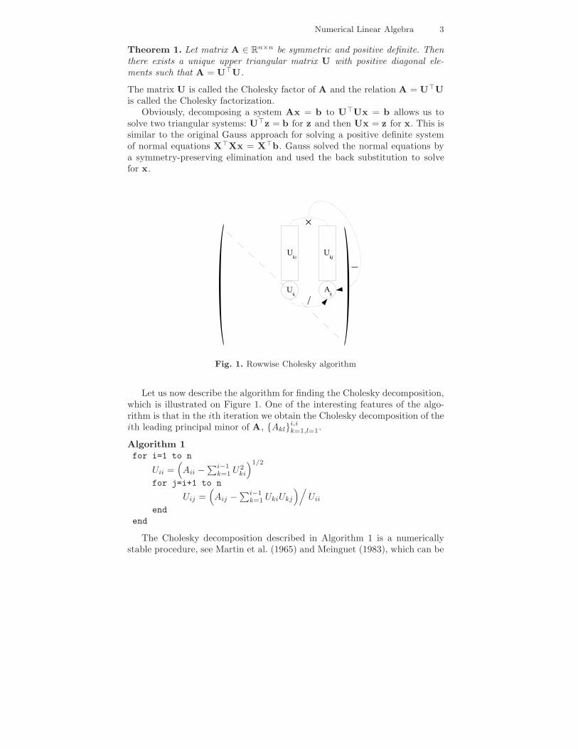
Fig. 1. Rowwise Cholesky algorithm

Let us now describe the algorithm for finding the Cholesky decomposition,which is illustrated on Figure 1. One of the interesting features of the algo-rithm is that in the ith iteration we obtain the Cholesky decomposition of theith leading principal minor of A, {Akl}i,i

k=1,l=1.

Algorithm 1for i=1 to n

Uii =(Aii −

∑i−1k=1 U2

ki

)1/2

for j=i+1 to n

Uij =(Aij −

∑i−1k=1 UkiUkj

)/Uii

endend

The Cholesky decomposition described in Algorithm 1 is a numericallystable procedure, see Martin et al. (1965) and Meinguet (1983), which can be


at the same time implemented in a very efficient way. Computed values Uij

can be stored in place of original Aij , and thus, no extra memory is needed.Moreover, let us note that while Algorithm 1 describes the rowwise decompo-sition (U is computed row by row), there are also a columnwise version and aversion with diagonal pivoting, which is also applicable to semidefinite matri-ces. Finally, there are also modifications of the algorithm, such as blockwisedecomposition, that are suitable for very large problems and parallelization;see Bjorck (1996), Gallivan et al. (1990) and Nool (1995).

1.2 LU Decomposition

The LU decomposition is another method reducing a square matrix A to aproduct of two triangular matrices (lower triangular L and upper triangularU). Contrary to the Cholesky decomposition, it does not require a positivedefinite matrix A, but there is no guarantee that L = U�.

Theorem 2. Let the matrix A ∈ Rn×n satisfy following conditions:

A11 �= 0, det(

A11 A12

A21 A22

)�= 0, det

A11 A12 A13

A21 A22 A23

A31 A32 A33

�= 0, . . . , detA �= 0.

Then there exists a unique lower triangular matrix L with ones on a diagonal,a unique upper triangular matrix U with ones on a diagonal and a uniquediagonal matrix D such that A = LDU.

Note that for any nonsingular matrix A there is always a row permutation Psuch that the permuted matrix PA satisfies the assumptions of Theorem 2.Further, a more frequently used version of this theorem factorizes A to alower triangular matrix L′ = LD and an upper triangular matrix U′ = U.Finally, Zou (1991) gave alternative conditions for the existence of the LUdecomposition: A ∈ R

n×n is nonsingular and A� is diagonally dominant (i.e.,|Aii| ≥

∑ni=1,i�=j |Aij | for j = 1, . . . , n).

Similarly to the Cholesky decomposition, the LU decomposition reducessolving a system of linear equations Ax = LUx = b to solving two triangularsystems: Lz = b, where z = Ux, and Ux = z.

Finding the LU decomposition of A is described in Algorithm 2. Since itis equivalent to solving a system of linear equations by the Gauss elimination,which searches just for U and ignores L, we refer a reader to Section 2,where its advantages (e.g., easy implementation, speed) and disadvantages(e.g., numerical instability without pivoting) are discussed.

Algorithm 2L = 0n,U = Infor i = 1 to n

for j = i to n


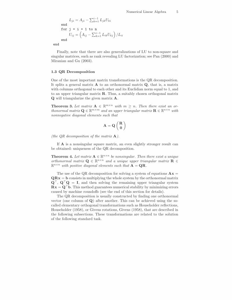
Lji = Aji −∑i−1

k=1 LjkUki

endfor j = i + 1 to n

Uij =(Aij −

∑i−1k=1 LikUkj

)/Lii

endend

Finally, note that there are also generalizations of LU to non-square andsingular matrices, such as rank revealing LU factorization; see Pan (2000) andMiranian and Gu (2003).

1.3 QR Decomposition

One of the most important matrix transformations is the QR decomposition.It splits a general matrix A to an orthonormal matrix Q, that is, a matrixwith columns orthogonal to each other and its Euclidian norm equal to 1, andto an upper triangular matrix R. Thus, a suitably chosen orthogonal matrixQ will triangularize the given matrix A.

Theorem 3. Let matrix A ∈ Rm×n with m ≥ n. Then there exist an or-

thonormal matrix Q ∈ Rm×m and an upper triangular matrix R ∈ R

n×n withnonnegative diagonal elements such that

A = Q(

R0

)

(the QR decomposition of the matrix A).

If A is a nonsingular square matrix, an even slightly stronger result canbe obtained: uniqueness of the QR decomposition.

Theorem 4. Let matrix A ∈ Rn×n be nonsingular. Then there exist a unique

orthonormal matrix Q ∈ Rn×n and a unique upper triangular matrix R ∈

Rn×n with positive diagonal elements such that A = QR.

The use of the QR decomposition for solving a system of equations Ax =QRx = b consists in multiplying the whole system by the orthonormal matrixQ�, Q�Q = I, and then solving the remaining upper triangular systemRx = Q�b. This method guarantees numerical stability by minimizing errorscaused by machine roundoffs (see the end of this section for details).

The QR decomposition is usually constructed by finding one orthonormalvector (one column of Q) after another. This can be achieved using the so-called elementary orthogonal transformations such as Householder reflections,Householder (1958), or Givens rotations, Givens (1958), that are described inthe following subsections. These transformations are related to the solutionof the following standard task.


Problem 1. Given a vector x ∈ Rm, x �= 0, find an orthogonal matrix M ∈

Rm×m such that M�x = ‖x‖2 ·e1, where e1 = (1, 0, . . . , 0)� denotes the first

unit vector.

In the rest of this section, we will first discuss how Householder reflections andGivens rotations can be used for solving Problem 1. Next, using these elemen-tary results, we show how one can construct the QR decomposition. Finally,we briefly mention the Gram-Schmidt orthogonalization method, which alsoprovides a way to find the QR decomposition.

Householder Reflections

The QR decomposition using Householder reflections (HR) was developed byGolub (1965). Householder reflection (or Householder transformation) is amatrix P,

P = I − 1cuu�, c =

12u�u, (3)

where u is a Householder vector. By definition, the matrix P is orthonormaland symmetric. Moreover, for any x ∈ R

m, it holds that

Px = x − 1c(u�x)u.

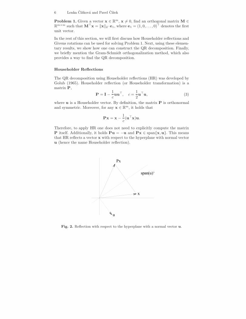
Therefore, to apply HR one does not need to explicitly compute the matrixP itself. Additionally, it holds Pu = −u and Px ∈ span{x,u}. This meansthat HR reflects a vector x with respect to the hyperplane with normal vectoru (hence the name Householder reflection).

Fig. 2. Reflection with respect to the hyperplane with a normal vector u.


To solve Problem 1 using some HR, we search for a vector u such that xwill be reflected to the x-axis. This holds for the following choice of u:

u = x + s1‖x‖2 · e1, s1 = 2I(x1 ≥ 0) − 1, (4)

where x1 = x�e1 denotes the first element of the vector x and I(·) representsan indicator. For this reflection, it holds that c from (3) equals ‖x‖2(‖x‖2 +|x1|) and Px = −s1‖x‖2 · e1 as one can verify by substituting (4) into (3).

Givens Rotations

A Givens rotation (GR) in m dimensions (or Givens transformation) is definedby an orthonormal matrix Rij(α) ∈ R

m×m,

Rij(α) =

1 0 · · · · · · · · · · · · 0

0. . .

...... c s

......

. . ....

... −s c...

.... . . 0

0 · · · · · · · · · · · · 0 1

i

j

(5)

where c = cosα and s = sinα for α ∈ R and 1 ≤ i < j ≤ n. Thus, the rotationRij(α) represents a plane rotation in the space spanned by the unit vectorsei and ej by an angle α. In two dimensions, rotation R12(α),

R12(α) =(

c s−s c

), c = cosα, s = sin α

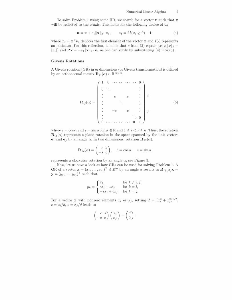
represents a clockwise rotation by an angle α; see Figure 3.Now, let us have a look at how GRs can be used for solving Problem 1. A

GR of a vector x = (x1, . . . , xm)� ∈ Rm by an angle α results in Rij(α)x =

y = (y1, . . . , ym)� such that

yk =

xk for k �= i, j,cxi + sxj for k = i,−sxi + cxj for k = j.

For a vector x with nonzero elements xi or xj , setting d = (x2i + x2

j )1/2,

c = xi/d, s = xj/d leads to(

c s−s c

) (xi

xj

)=

(d0

).


Fig. 3. Rotation of x in a plane by an angle α.

Thus, using GR with this specific choice of c and s (referred further as R0ij)

implies that the jth component of the vector x vanishes. Similarly to HRs,it is not necessary to explicitly construct the whole matrix P to transformx since the rotation is fully described by only two numbers: c and s. Thiselementary rotation R0

ij does not however constitute a solution to Problem 1yet: we need to combine more of them.

The next step employs a simple fact that the pre- or postmultiplication ofa vector x or a matrix A by any GR Rij(α) affects only the ith and jth rowsand columns, respectively. Hence, one can combine several rotations withoutone rotation spoiling the result of another rotation. (Consequently, GRs aremore flexible than HRs). Two typical ways how GRs are used for solvingProblem 1 mentioned in Section 1.3 follow.

1. R01nR0

1,n−1 . . .R013R

012x = de1. Here the kth component of the vector x

vanishes after the Givens rotation R01k. The previously zeroed elements

x2, . . . , xk−1 are not changed because rotation R1k affects only the firstand kth component.

2. R012R

023 . . .R0

n−1,nx = de1. Here the kth component vanishes by the ro-tation Rk−1,k.

Finally, there are several algorithms for computing the Givens rotationsthat improve over the straightforward evaluation of R0

ijx. A robust algorithmminimizing the loss of precision is given in Bjorck (1996). An algorithm min-imizing memory requirements was proposed by Stewart (1976). On the otherhand, Gentleman (1973) and Hammarling (1974) proposed modifications aim-ing to minimize the number of arithmetic operations.


QR Decomposition by Householder Reflections or GivensRotations

An appropriate combination of HRs or GRs, respectively, can be used tocompute the QR decomposition of a given matrix A ∈ R

m×n, m ≥ n, ina following way. Let Qi, i = 1, . . . , n − 1, denote an orthonormal matrix inR

m×m such that premultiplication of B = Qi−1 · · ·Q1A by Qi can zero allelements in the ith column that are below the diagonal and such that theprevious columns 1, . . . , i − 1 are not affected at all. Such a matrix can be ablockwise diagonal matrix with blocks being the identity matrix Ii−1 and amatrix M solving Problem 1 for the vector composed of elements in the ithcolumn of B that lie on and below the diagonal. The first part Ii−1 guaranteesthat the columns 1, . . . , i − 1 of matrix B are not affected by multiplication,whereas the second block M transforms all elements in the ith column thatare below the diagonal to zero. Naturally, matrix M can be found by meansof HRs or GRs as described in previous paragraphs.

This way, we construct a series of matrices Q1, . . . ,Qn such that

Qn · · ·Q1A =(

R0

).

Since all matrices Q1, . . . ,Qn are orthonormal, Qt = Qn · · ·Q1 is also or-thonormal and its inverse equals its transpose: Q−1

t = Q�t . Hence,

A = (Qn · · ·Q1)�(

R0

)= Q

(R0

)

as described in Theorem 3.We describe now the QR algorithm using HRs or GRs. Let M(x) denote

the orthonormal matrix from Problem 1 constructed for a vector x by one ofthe discussed methods.

Algorithm 3Q = ImR = Afor i = 1 to n

x = {Rki}mk=i

Qi =(

Ii−1 00 M(x)

)

Q = QiQR = QiR

endQ = Q�

R = {Rij}n,ni=1,j=1

There are also modifications of this basic algorithm employing pivotingfor better numerical performance and even revealing rank of the system, see


Hong and Tan (1992) and Higham (2000) for instance. An error analysis ofthe QR decomposition by HRs and GRs are given by Gentleman (1975) andHigham (2000), respectively.

Gram-Schmidt Orthogonalization

Given a nonsingular matrix A ∈ Rm×n, m ≥ n, the Gram-Schmidt orthogo-

nalization constructs a matrix Q such that the columns of Q are orthonormalto each other and span the same space as the columns of A. Thus, A can beexpressed as Q multiplied by another matrix R, whereby the Gram-Schmidtorthogonalization process (GS) ensures that R is an upper triangular matrix.Consequently, GS can be used to construct the QR decomposition of a matrixA. A survey of GS variants and their properties is given by Bjorck (1994).

The classical Gram-Schmidt (CGS) process constructs the orthonormalbasis stepwise. The first column Q1 of Q is simply normalized A1. Havingconstructed a orthonormal base Q1:k = {Q1, . . . ,Qk}, the next column Qk+1

is proportional to Ak+1 minus its projection to the space span{Q1:k}. Thus,Qk+1 is by its definition orthogonal to span{Q1:k}, and at the same time, thefirst k columns of A and Q span the same linear space. The elements of thetriangular matrix R from Theorem 3 are then coordinates of the columns ofA given the columns of Q as a basis.

Algorithm 4for i = 1 to n

for j = 1 to i - 1Rji = Q�

j Ai

endQi = Ai −

∑i−1j=1 RjiQj

Rii = (Q�i Qi)1/2

Qi = Qi/Rii

end

Similarly to many decomposition algorithms, also CGS allows a memoryefficient implementation since the computed orthonormal columns of Q canrewrite the original columns of A. Despite this feature and mathematical cor-rectness, the CGS algorithm does not always behave well numerically becausenumerical errors can very quickly accumulate. For example, an error madein computing Q1 affects Q2, errors in both of these terms (although causedinitially just by an error in Q1) adversely influence Q3 and so on. Fortunately,there is a modified Gram-Schmidt (MGS) procedure, which prevents such anerror accumulation by subtracting linear combinations of Qk directly fromA before constructing following orthonormal vectors. (Surprisingly, MGS ishistorically older than CGS.)

Algorithm 5for i = 1 to n


Qi = Ai

Rii = (Q�i Qi)1/2

Qi = Qi/Rii

for j = i + 1 to nRji = Q�

i Aj

Aj = Aj − RijQi

endend

Apart from this algorithm (the row version of MGS), there are also acolumn version of MGS by Bjorck (1994) and MGS modifications employingiterative orthogonalization and pivoting by Dax (2000). Numerical superiorityof MGS over CGS was experimentally established already by Rice (1966). Thisresult is also theoretically supported by the GS error analysis in Bjorck (1994),who uncovered numerical equivalence of the QR decompositions done by MGSand HRs.

1.4 Singular Value Decomposition

The singular value decomposition (SVD) plays an important role in numericallinear algebra and in many statistical techniques as well. Using two orthonor-mal matrices, SVD can diagonalize any matrix A and the results of SVDcan tell a lot about (numerical) properties of the matrix. (This is closely re-lated to the eigenvalue decomposition: any symmetric square matrix A canbe diagonalized, A = VDV�, where D is a diagonal matrix containing theeigenvalues of A and V is an orthonormal matrix.)

Theorem 5. Let A ∈ Rm×n be a matrix of rank r. Then there exist orthonor-

mal matrices U ∈ Rm×m and V ∈ R

n×n and a diagonal matrix D ∈ Rm×n,

with the diagonal elements σ1 ≥ σ2 ≥ · · · ≥ σr > σr+1 = . . . = σmin{m,n} = 0,such that A = UDV�.

Numbers σ1, . . . , σmin{m,n} represent the singular values of A. Columns Ui

and Vi of matrices U and V are called the left and right singular vectors ofA associated with singular value σi, respectively, because AVi = σiUi andU�

i A = σiV�i , i = 1, . . . , min{m, n}.

Similarly to the QR decomposition, SVD offers a numerically stable wayto solve a system of linear equations. Given a system Ax = UDV�x = b,one can transform it to U�Ax = DV�x = U�b and solve it in two trivialsteps: first, finding a solution z of Dz = U�b, and second, setting x = Vz,which is equivalent to V�x = z.

On the other hand, the power of SVD lies in its relation to many impor-tant matrix properties; see Trefethen and Bau (1997), for instance. First ofall, the singular values of a matrix A are equal to the (positive) square rootsof the eigenvalues of A�A and AA�, whereby the associated left and rightsingular vectors are identical with the corresponding eigenvectors. Thus, one


can compute the eigenvalues of A�A directly from the original matrix A.Second, the number of nonzero singular values equals the rank of a matrix.Consequently, SVD can be used to find an effective rank of a matrix, to checka near singularity and to compute the condition number of a matrix. That is,it allows to assess conditioning and sensitivity to errors of a given system ofequations. Finally, let us note that there are far more uses of SVD: identifica-tion of the null space of A, null(A) = span{Vk+1, . . . ,Vn}; computation ofthe matrix pseudo-inverse, A− = VD−U�; low-rank approximations and soon. See Bjorck (1996) and Trefethen and Bau (1997) for details.

Let us now present an overview of algorithms for computing the SVDdecomposition, which are not described in details due to their extent. Thefirst stable algorithm for computing the SVD was suggested by Golub andKahan (1965). It involved reduction of a matrix A to its bidiagonal formby HRs, with singular values and vectors being computed as eigenvalues andeigenvectors of a specific tridiagonal matrix using a method based on Sturmsequences. The final form of the QR algorithm for computing SVD, whichhas been the preferred SVD method for dense matrices up to now, is dueto Golub and Reinsch (1970); see Anderson et al. (1999), Bjorck (1996) orGentle (1998) for the description of the algorithm and some modifications.An alternative approach based on Jacobi algorithm was given by Hari andVeselic (1987). Latest contributions to the pool of computational methods forSVD, including von Matt (1995), Demmel et al. (1999) and Higham (2000),aim to improve the accuracy of singular values and computational speed usingrecent advances in the QR decomposition.

1.5 Matrix Inversion

In previous sections, we described how matrix decompositions can be used forsolving systems of linear equations. Let us now discuss the use of matrix de-compositions for inverting a nonsingular squared matrix A ∈ R

n×n, althoughmatrix inversion is not needed very often. All discussed matrix decomposi-tion construct two or more matrices A1, . . . ,Ad such that A = A1 · . . . ·Ad,where matrices Al, l = 1, . . . , d, are orthonormal, triangular, or diagonal. Be-cause A−1 = A−1

d · . . . · A−11 , we just need to be able to invert orthonormal

and triangular matrices (a diagonal matrix is a special case of a triangularmatrix).

First, an orthonormal matrix Q satisfies by definition Q�Q = QQ� = In.Thus, inversion is in this case equivalent to the transposition of a matrix:Q−1 = Q�.

Second, inverting an upper triangular matrix U can be done by solvingdirectly XU = In, which leads to the backward substitution method. LetX = {Xij}n,n

i=1,j=1 denote the searched for inverse matrix U−1.

Algorithm 6X = 0n


for i = n to 1Xii = 1/Uii

for j = i + 1 to n

Xij = −(∑j

k=i+1 XkjUik

)/Ujj

endend

The inversion of a lower triangular matrix L can be done analogously: thealgorithm is applied to L�, that is, Uij is replaced by Lji for i, j = 1, . . . , n.

There are several other algorithms available such as forward substitution orblockwise inversion. Designed for a faster and more (time) efficient computa-tion, their numerical behavior does not significantly differ from the presentedalgorithm. See Croz and Higham (1992) for an overview and numerical study.

2 Direct Methods for Solving Linear Systems

A system of linear equations can be written in the matrix notation as

Ax = b, (6)

where A denotes the coefficient matrix, b is the right-hand side, and x rep-resents the solution vector we search for. The system (6) has a solution if andonly if b belongs to the vector space spanned by the columns of A.

• If m < n, that is, the number of equations is smaller than the number ofunknown variables, or if m ≥ n but A does not have a full rank (whichmeans that some equations are linear combinations of the other ones),the system is underdetermined and there are either no solution at all orinfinitely many of them. In the latter case, any solution can be written as asum of a particular solution and a vector from the nullspace of A. Findingthe solution space can involve the SVD decomposition (Section 1.4).

• If m > n and the matrix A has a full rank, that is, if the number ofequations is greater than the number of unknown variables, there is gen-erally no solution and the system is overdetermined. One can search somex such that the distance between Ax and b is minimized, which leads tothe linear least-squares problem if distance is measured by L2 norm; seeChapter ??.

• If m = n and the matrix A is nonsingular, the system (6) has a uniquesolution. Methods suitable for this case will be discussed in the rest of thissection as well as in Section 3.

¿From here on, we concentrate on systems of equations with unique solutions.There are two basic classes of methods for solving system (6). The first

class is represented by direct methods. They theoretically give an exact solu-tion in a (predictable) finite number of steps. Unfortunately, this does not have


to be true in computational praxis due to rounding errors: an error made inone step spreads in all following steps. Classical direct methods are discussedin this section. Moreover, solving an equation system by means of matrix de-compositions, as discussed in Section 1, can be classified as a direct method aswell. The second class is called iterative methods, which construct a series ofsolution approximations that (under some assumptions) converges to the solu-tion of the system. Iterative methods are discussed in Section 3. Finally, notethat some methods are on the borderline between the two classes; for example,gradient methods (Section 3.5) and iterative refinement (Section 2.2).

Further, the direct methods discussed in this section are not necessarilyoptimal for an arbitrary system (6). Let us deal with the main exceptions.First, even if a unique solution exist, numerical methods can fail to find thesolution: if the number of unknown variables n is large, rounding errors canaccumulate and result in a wrong solution. The same applies very much tosystems with a nearly singular coefficient matrix. One alternative is to useiterative methods (Section 3), which are less sensitive to these problems. An-other approach is to use the QR or SVD decompositions (Section 1), which cantransform some nearly singular problems to nonsingular ones. Second, verylarge problems including hundreds or thousands of equations and unknownvariables may be very time demanding to solve by standard direct methods.On the other hand, their coefficient matrices are often sparse, that is, most oftheir elements are zeros. Special strategies to store and solve such problemsare discussed in Section 5.

To conclude these remarks, let us mention a close relation between solvingthe system (6) and computing the inverse matrix A−1:

• having an algorithm that for a matrix A computes A−1, we can find thesolution to (6) as x = A−1b;

• an algorithm solving the system (6) can be used to compute A−1 as follows.Solve n linear systems Axi = ei, i = 1, . . . , n (or the corresponding systemwith multiple right-hand sides), where ei denotes the ith unit vector. ThenA−1 = (x1, . . . ,xn).

In the rest of this section, we concentrate on the Gauss-Jordan elimination(Section 2.1) and its modifications and extensions, such as iterative refinement(Section 2.2). A wealth of information on direct methods can be found inmonographs Axelsson (1994), Gentle (1998) and Golub and van Loan (1996).

2.1 Gauss-Jordan Elimination

In this subsection, we will simultaneously solve the linear systems

Ax1 = b1, Ax2 = b2, . . . , Axk = bk

and a matrix equation AX = B, where X,B ∈ Rn×l (its solution is X =

A−1B, yielding the inverse A−1 for a special choice B = In). They can bewritten as a linear matrix equation


A[x1|x2| . . . |xk|X] = [b1|b2| . . . |bk|B], (7)

where the operator | stands for column augmentation.The Gauss-Jordan elimination (GJ) is based on elementary operations that

do not affect the solution of an equation system. The solution of (7) will notchange if we perform any of the following operations:

• interchanging any two rows of A and the corresponding rows of bi’s andB, i = 1, . . . , k;

• multiplying a row of A and the same row of bi’s and B by a nonzeronumber, i = 1, . . . , k;

• adding to a chosen row of A and the same row of bi’s and B a linearcombination of other rows, i = 1, . . . , k.

Interchanging any two columns of A is possible too, but it has to be followedby interchanging the corresponding rows of all solutions xi and X as well asof right sides bi and B, i = 1, . . . , k. Each row or column operation describedabove is equivalent to the pre- or postmultiplication of the system by a certainelementary matrix R or C, respectively, that are results of the same operationapplied to the identity matrix In.

GJ is a technique that applies one or more of these elementary operationsto (7) so that A becomes the identity matrix In. Simultaneously, the right-hand side becomes the set of solutions. Denoting Ri, i = 1, . . . , O, the matricescorresponding to the ith row operation, the combination of all operations hasto constitute inverse A−1 = RO · . . . · R3R2R1 and hence x = RO · . . . ·R3R2R1b. The exact choice of these elementary operation is described inthe following paragraph.

Pivoting in Gauss-Jordan Elimination

Let us now discuss several well-known variants of the Gauss-Jordan elimina-tion. GJ without pivoting does not interchange any rows or columns; onlymultiplication and addition of rows are permitted. First, nonzero nondiagonalelements in the first column A1 are eliminated: the first row of (7) is dividedby its diagonal element A11 and the Ai1-multiple of the modified first row issubtracted from the ith row, i = 2, . . . , n. We can proceed the same way forall n columns of A, and thus, transform A to the identity matrix In. It iseasy to see that the method fails if the diagonal element in a column to beeliminated, the so-called pivot, is zero in some step. Even if this is not thecase, one should be aware that GJ without pivoting is numerically unstable.

On the other hand, the GJ method becomes stable when using pivoting.This means that one can interchange rows (partial pivoting) or rows andcolumns (full pivoting) to put a suitable matrix element to the position of thecurrent pivot. Since it is desirable to keep the already constructed part of theidentify matrix, only rows below and columns right to the current pivot areconsidered. GJ with full pivoting is numerically stable. From the application


point of view, GJ with partial pivoting is numerically stable too, althoughthere are artificial examples where it fails. Additionally, the advantage ofpartial pivoting (compared to full pivoting) is that it does not change theorder of solution components.

There are various strategies to choose a pivot. A very good choice is thelargest available element (in absolute value). This procedure depends howeveron the original scaling of the equations. Implicit pivoting takes scaling intoaccount and chooses a pivot as if the original system were rescaled so that thelargest element of each row would be equal to one.

Finally, let us add several concluding remarks on efficiency of GJ andits relationship to matrix decompositions. As shown, GJ can efficiently solveproblems with multiple right-hand sides known in advance and compute A−1

at the same time. On the other hand, if it is necessary to solve later a new sys-tem with the same coefficient matrix A but a new right-hand side b, one hasto start the whole elimination process again, which is time demanding, or com-pute A−1b using the previously computed inverse matrix A−1, which leadsto further error accumulation. In praxis, one should prefer matrix decompo-sitions, which do not have this drawback. Specifically, the LU decomposition(Section 1.2) is equivalent to GJ (with the same kind of pivoting applied inboth cases) and allows us to repeatedly solve systems with the same coefficientmatrix in an efficient way.

2.2 Iterative Refinement

In the introduction to Section 2, we noted that direct methods are rathersensitive to rounding errors. Iterative refinement offers a way to improve thesolution obtained by any direct method, unless the system matrix A is tooill-conditioned or even singular.

Let x1 denote an initially computed (approximate) solution of (6). Itera-tive refinement is a process constructing a series xi, i = 1, 2, . . . , as describedin Algorithm 7. First, given a solution xi, the residuum ri = Axi −b is com-puted. Then, one obtains the correction ∆xi by solving the original systemwith residuum ri on the right-hand side.

Algorithm 7Repeat for i = 1, 2, . . .

compute ri = b − Axi

solve A∆xi = ri for ∆xi

set xi+1 = xi + ∆xi

until the desired precision is achieved.

It is reasonable to carry out the computation of residuals ri in a higher preci-sion because a lot of cancellation occurs if xi is a good approximation. Never-theless, provided that the coefficient matrix A is not too ill-conditioned, Skeel(1980) proved that GJ with partial pivoting and only one step of iterative re-finement computed in a fixed precision is stable (it has a relative backward


error proportional to the used precision). In spite of this result, one can rec-ommend to use iterative refinement repeatedly until the desired precision isreached.

Additionally, an important feature of iterative refinement is its low com-putational costs. Provided that a system is solved by means of decompositions(e.g., GJ is implemented as the LU decomposition), a factorization of A isavailable already after computing the initial solution x1. Subsequently, solvingany system with the same coefficient matrix A, such as A∆xi = ri, can bedone fast and efficiently and the computational costs of iterative refinementare small.

3 Iterative Methods for Solving Linear Systems

Direct methods for solving linear systems theoretically give the exact solutionin a finite number of steps, see Section 2. Unfortunately, this is rarely truein applications because of rounding errors: an error made in one step spreadsfurther in all following steps! Contrary to direct methods, iterative methodsconstruct a series of solution approximations such that it converges to the ex-act solution of a system. Their main advantage is that they are self-correcting,see Section 3.1.

In this section, we first discuss general principles of iterative methods thatsolve linear system (6), Ax = b, whereby we assume that A ∈ R

n×n and thesystem has exactly one solution xe (see Section 2 for more details on othercases). Later, we describe most common iterative methods: the Jacobi, Gauss-Seidel, successive overrelaxation, and gradient methods (Sections 3.2–3.5).Monographs containing detailed discussion of these methods include Bjorck(1996), Golub and van Loan (1996) and Hackbusch (1994). Although we treatthese methods separately from the direct methods, let us mention here thatiterative methods can usually benefit from a combination with the Gausselimination, see Milaszewicz (1987) and Allanelli and Hadjidimos (2004), forinstance.

To unify the presentation of all methods, let D, L, and U denote the di-agonal, lower triangular and upper triangular parts of a matrix A throughoutthis section:

Dij ={

Aij for i = j,0 otherwise; Lij =

{Aij for i > j,0 otherwise; Uij =

{Aij for i < j,0 otherwise.

3.1 General Principle of Iterative Methods for Linear Systems

An iterative method for solving a linear system Ax = b constructs an iter-ation series xi, i = 0, 1, 2, . . . , that under some conditions converges to theexact solution xe of the system (Axe = b). Thus, it is necessary to choosea starting point x0 and iteratively apply a rule that computes xi+1 from analready known xi.


A starting vector x0 is usually chosen as some approximation of x. (Luck-ily, its choice cannot cause divergence of a convergent method.) Next, givenxi, i ∈ N, the subsequent element of the series is computed using a rule of theform

xi+1 = Bixi + Cib, i = 0, 1, 2, . . . , (8)

where Bi,Ci ∈ Rn×n, i ∈ N, are matrix series. Different choices of Bi and Ci

define different iterative methods.Let us discuss now a minimal set of conditions on Bi and Ci in (8) that

guarantee the convergence of an iterative method. First of all, it has to holdthat Bi + CiA = In for all i ∈ N, or equivalently,

xe = Bixe + Cib = (Bi + CiA)xe, i ∈ N. (9)

In other words, once the iterative process reaches the exact solution xe, allconsecutive iterations should stay equal to xe and the method cannot departfrom this solution. Second, starting from a point x0 �= xe, we have to ensurethat approximations xi will converge to xe as i increases.

Theorem 6. An iteration series xi given by (8) converges to the solution ofsystem (6) for any chosen x0 iff

limi→∞

BiBi−1 . . .B0 = 0.

In praxis, stationary iterative methods are used, that is, methods withconstant Bi = B and Ci = C, i ∈ N. Consequently, an iteration series is thenconstructed using

xi+1 = Bxi + Cb, i = 0, 1, 2, . . . (10)

and the convergence condition in Theorem 6 has a simpler form.

Theorem 7. An iteration series xi given by (10) converges to the solution ofsystem (6) for any chosen x0 iff the spectral radius ρ(B) < 1, where ρ(B) =maxi=1,...,n |λi| and λ1, . . . , λn represent the eigenvalues of B.

Note that the convergence condition ρ(B) < 1 holds, for example, if ‖B‖ < 1in any matrix norm. Moreover, Theorem 7 guarantees the self-correcting prop-erty of iterative methods since convergence takes place independent of thestarting value x0. Thus, if computational errors adversely affect xi during theith iteration, xi can be considered as a new starting vector and the itera-tive method will further converge. Consequently, the iterative methods are ingeneral more robust than the direct ones.

Apparently, such an iterative process can continue arbitrarily long unlessxi = xe at some point. This is impractical and usually unnecessary. Therefore,one uses stopping (or convergence) criteria that stop the iterative processwhen a pre-specified condition is met. Commonly used stopping criteria are


based on the change of the solution or residual vector achieved during oneiteration. Specifically, given a small ε > 0, the iterative process is stoppedafter the ith iteration when ‖xi − xi−1‖ ≤ ε, ‖ri − ri−1‖ ≤ ε, or ‖ri‖ ≤ ε,where ri = Axi −b is a residual vector. Additionally, a maximum acceptablenumber of iterations is usually specified.

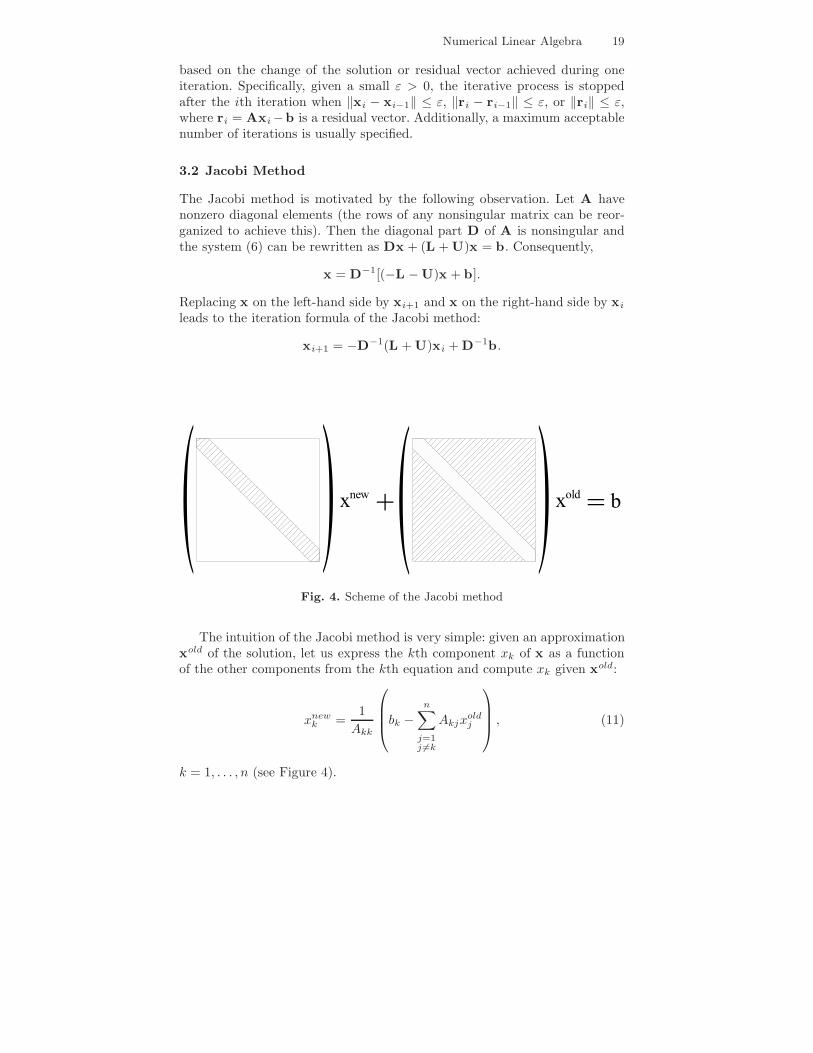
3.2 Jacobi Method

The Jacobi method is motivated by the following observation. Let A havenonzero diagonal elements (the rows of any nonsingular matrix can be reor-ganized to achieve this). Then the diagonal part D of A is nonsingular andthe system (6) can be rewritten as Dx + (L + U)x = b. Consequently,

x = D−1[(−L − U)x + b].

Replacing x on the left-hand side by xi+1 and x on the right-hand side by xi

leads to the iteration formula of the Jacobi method:

xi+1 = −D−1(L + U)xi + D−1b.

Fig. 4. Scheme of the Jacobi method

The intuition of the Jacobi method is very simple: given an approximationxold of the solution, let us express the kth component xk of x as a functionof the other components from the kth equation and compute xk given xold:

xnewk =

1Akk

bk −

n∑j=1j �=k

Akjxoldj

, (11)

k = 1, . . . , n (see Figure 4).


The Jacobi method converges for any starting vector x0 as long asρ(D−1(L + U)) < 1, see Theorem 7. This condition is satisfied for a rela-tively big class of matrices including diagonally dominant matrices (matricesA such that

∑nj=1,j �=i |Aij | ≤ |Aii| for i = 1, . . . , n), and symmetric matrices

A such that D, A = L + D + U, and −L + D − U are all positive definite.Although there are many improvements to the basic principle of the Jacobimethod in terms of convergence to xe, see Sections 3.3 and 3.4, its advantageis an easy and fast implementation (elements of a new iteration xi can becomputed independently of each other).

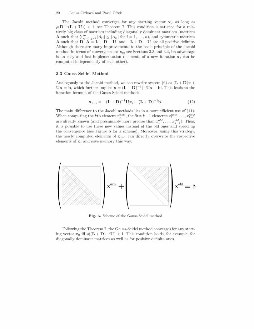
3.3 Gauss-Seidel Method

Analogously to the Jacobi method, we can rewrite system (6) as (L + D)x +Ux = b, which further implies x = (L + D)−1[−Ux + b]. This leads to theiteration formula of the Gauss-Seidel method:

xi+1 = −(L + D)−1Uxi + (L + D)−1b. (12)

The main difference to the Jacobi methods lies in a more efficient use of (11).When computing the kth element xnew

k , the first k−1 elements xnew1 , . . . , xnew

k−1

are already known (and presumably more precise than xold1 , . . . , xold

k−1). Thus,it is possible to use these new values instead of the old ones and speed upthe convergence (see Figure 5 for a scheme). Moreover, using this strategy,the newly computed elements of xi+1 can directly overwrite the respectiveelements of xi and save memory this way.

Fig. 5. Scheme of the Gauss-Seidel method

Following the Theorem 7, the Gauss-Seidel method converges for any start-ing vector x0 iff ρ((L + D)−1U) < 1. This condition holds, for example, fordiagonally dominant matrices as well as for positive definite ones.


3.4 Successive Overrelaxation Method

The successive overrelaxation (SOR) method aims to further refine the Gauss-Seidel method. The Gauss-Seidel formula (12) can be rewritten as

xi+1 = xi − D−1[{Lxi+1 + (D + U)xi} − b] = xi − ∆i,

which describes the difference ∆i between xi+1 and xi expressed for the kthelement of xi(+1) from the kth equation, k = 1, . . . , n. The question SORposes is whether the method can converge faster if we “overly” correct xi+1

in each step; that is, if xi is corrected by a multiple ω of ∆i in each iteration.This idea leads to the SOR formula:

xi+1 = xi − ωD−1[{Lxi+1 + (D + U)xi} − b],

or in the form (10),

xi+1 = (D + ωL)−1{(1 − ω)D − ωU}xi + ω(D + ωL)−1b. (13)

The parameter ω is called the (over)relaxation parameter and it can be shownthat SOR converges only for ω ∈ (0, 2), a result derived by Kahan (1958).

A good choice of parameter ω can speed up convergence, as measured bythe spectral radius of the corresponding iteration matrix B (see Theorem 7;a lower spectral radius ρ(B) means faster convergence). There is a choice ofliterature devoted to the optimal setting of relaxation parameter: see Hadjidi-mos (2000) for a recent overview of the main results concerning SOR. We justpresent one important result, which is due to Young (1954).

Definition 1. A matrix A is said to be two-cyclic consistently ordered if theeigenvalues of the matrix M(α) = αD−1L + α−1D−1U, α �= 0, are indepen-dent of α.

Theorem 8. Let the matrix A be two-cyclic consistently ordered. Let the re-spective Gauss-Seidel iteration matrix B = −(L + D)−1U have the spectralradius ρ(B) < 1. Then the optimal relaxation parameter ω in SOR is givenby

ωopt =2

1 +√

1 − ρ(B)

and for this optimal value it holds ρ(B; ωopt) = ωopt − 1.

Using SOR with the optimal relaxation parameter significantly increasesthe rate of convergence. Note however that the convergence acceleration isobtained only for ω very close to ωopt. If ωopt cannot be computed exactly, itis better to take ω slightly larger rather than smaller. Golub and van Loan(1996) describe an approximation algorithm for ρ(B).

On the other hand, if the assumptions of Theorem 8 are not satisfied, onecan employ the symmetric SOR (SSOR), which performs the SOR iteration


twice: once as usual, see (13), and once with interchanged L and U. SSORrequires more computations per iteration and usually converges slower, butit works for any positive definite matrix and can be combined with variousacceleration techniques. See Bjorck (1996) and Hadjidimos (2000) for details.

3.5 Gradient methods

Gradient iterative methods are based on the assumption that A is a symmetricpositive definite matrix A. They use this assumption to reformulate (6) as aminimization problem: xe is the only minimum of the quadratic form

Q(x) =12x�Ax − x�b.

Given this minimization problem, gradient methods construct an iterationseries of vectors converging to xe using the following principle. Having the ithapproximation xi, choose a direction vi and find a number αi such that thenew vector

xi+1 = xi + αivi

is a minimum of Q(x) on the line xi + αvi, α ∈ R. Various choices of di-rections vi then render different gradient methods, which are in general non-stationary (vi changes in each iteration). We discuss here three methods: theGauss-Seidel (as a gradient method), steepest descent and conjugate gradientsmethods.

Gauss-Seidel Method as a Gradient Method

Interestingly, the Gauss-Seidel method can be seen as a gradient method forthe choice

vkn+i = ei, k = 0, 1, 2, . . . , i = 1, . . . , n,

where ei denotes the ith unit vector. The kth Gauss-Seidel iteration corre-sponds to n subiterations with vkn+i for i = 1, . . . , n.

Steepest Descent Method

The steepest descent method is based on the direction vi given by the gradientof Q(x) at xi. Denoting the residuum of the ith approximation ri = b−Axi,the iteration formula is

xi+1 = xi +r�i ri

r�i Ariri,

where ri represents the direction vi and its coefficient is the Q(x)-minimizingchoice of αi. By definition, this method reduces Q(xi) at each step, but itis not very effective. The conjugate gradient method discussed in the nextsubsection will usually perform better.


Conjugate Gradient Method

In the conjugate gradient (CG) method proposed by Hestenes and Stiefel(1952), the directions vi are generated by the A-orthogonalization of residuumvectors. Given a symmetric positive definite matrix A, A-orthogonalizationis a procedure that constructs a series of linearly independent vectors vi suchthat v�

i Avj = 0 for i �= j (conjugacy or A-orthogonality condition). It canbe used to solve the system (6) as follows (ri = b−Axi represents residuals).

Algorithm 8v0 = r0 = b − Ax0

doαi = (v�

i ri)/(v�i Avi)

xi+1 = xi + αivi

ri+1 = ri − αiAvi

βi = −(v�i Ari+1)/(v�

i Avi)vi+1 = ri+1 + βivi

until a stop criterion holds

An interesting theoretic property of CG is that it reaches the exact solutionin at most n steps because there are not more than n (A-)orthogonal vectors.Thus, CG is not a truly iterative method. (This does not have to be the caseif A is a singular or non-square matrix, see Kammerer and Nashed, 1972.)On the other hand, it is usually used as an iterative method, because it cangive a solution within the given accuracy much earlier than after n iterations.Moreover, if the approximate solution xn after n iterations is not accurateenough (due to computational errors), the algorithm can be restarted with x0

set to xn. Finally, let us note that CG is attractive for use with large sparsematrices because it addresses A only by its multiplication by a vector. Thisoperation can be done very efficiently for a properly stored sparse matrix, seeSection 5.

The principle of CG has many extensions that are applicable also for non-symmetric nonsingular matrices: for example, generalized minimal residual,Saad and Schultz (1986); (stabilized) biconjugate gradients, Vorst (1992); orquasi-minimal residual, Freund and Nachtigal (1991).

4 Eigenvalues and Eigenvectors

In this section, we deal with methods for computing eigenvalues and eigen-vectors of a matrix A ∈ R

n×n. First, we discuss a simple power method forcomputing one or few eigenvalues (Section 4.1). Next, we concentrate on meth-ods performing the complete eigenanalysis, that is, finding all eigenvalues (theJacobi, QR, and LR methods in Sections 4.2–4.5). Finally, we briefly describea way to improve already computed eigenvalues and to find the correspondingeigenvector. Additionally, note that eigenanalysis can be also done by means


of SVD, see Section 1.4. For more details on the described as well as someother methods, one can consult monographs by Gentle (1998), Golub and vanLoan (1996), Press et al. (1992) and Stoer and Bulirsch (2002).

Before discussing specific methods, let us describe the principle commonto most of them. We assume that A ∈ R

n×n has eigenvalues |λ1| ≥ |λ2| ≥· · · ≥ |λn|. To find all eigenvalues, we transform the original matrix A to asimpler matrix B such that it is similar to A (recall that matrices A and Bare similar if there is a matrix T such that B = T−1AT). The similarityof A and B is crucial since it guarantees that both matrices have the sameeigenvalues and their eigenvectors follow simple relation: if g is an eigenvec-tor of B corresponding to its eigenvalue λ, then Tg is an eigenvector of Acorresponding to the same eigenvalue λ.

There are two basic strategies to construct a similarity transformation Bof the original matrix A. First, one can use a series of simple transformations,such as GRs, and eliminate elements of A one by one (see the Jacobi method,Section 4.2). This approach is often used to transform A to its tridiagonalor upper Hessenberg forms. (Matrix B has the upper Hessenberg form ifit is an upper triangular except for the first subdiagonal; that is, Aij = 0for i > j + 1, where i, j = 1, . . . , n). Second, one can also factorize A intoA = FLFR and switch the order of factors, B = FRFL (similarity of A andB follows from B = FRFL = F−1

L AFL). This is used for example by the LRmethod (Section 4.5). Finally, there are methods combining both approaches.

4.1 Power Method

In its basic form, the power method aims at finding only the largest eigenvalueλ1 of a matrix A and the corresponding eigenvector. Let us assume that thematrix A has a dominant eigenvalue (|λ1| > |λ2|) and n linearly independenteigenvectors.

The power method constructs two series ci and xi, i ∈ N, that convergeto λ1 and to the corresponding eigenvector g1, respectively. Starting froma vector x0 that is not orthogonal to g1, one only has to iteratively com-pute Axi and split it to its norm ci+1 and the normalized vector xi+1,see Algorithm 9. Usually, the Euclidian (ci+1 = ‖Axi‖2) and maximum(ci+1 = maxj=1,...,n |(Axi)j |) norms are used.

Algorithm 9i = 0do

i = i + 1xi+1 = Axi

ci+1 = ‖Axi+1‖xi+1 = xi+1/ci+1

until a stop criterion holds


Although assessing the validity of assumptions is far from trivial, one canusually easily recognize whether the method converges from the behaviour ofthe two constructed series.

Furthermore, the power method can be extended to search also for othereigenvalues; for example, the smallest one and the second largest one. First, ifA is nonsingular, we can apply the power method to A−1 to find the smallesteigenvalue λn because 1/λn is the largest eigenvalue of A−1. Second, if weneed more eigenvalues and λ1 is already known, we can use a reduction methodto construct a matrix B that has the same eigenvalues and eigenvectors as Aexcept for λ1, which is replaced by zero eigenvalue. To do so, we need to finda (normalized) eigenvector h1 of A� corresponding to λ1 (A and A� havethe same eigenvalues) and to set B = A − λ1h1h�

1 . Naturally, this processcan be repeated to find the third and further eigenvalues.

Finally, let us mention that the power method can be used also for somematrices without dominant eigenvalue (e.g., matrices with λ1 = · · · = λp forsome 1 < p ≤ n). For further extensions of the power method see Sidi (1989),for instance.

4.2 Jacobi Method

For a symmetric matrix A, the Jacobi method constructs a series of orthog-onal matrices Ri, i ∈ N, such that the matrix Ti = R�

i . . .R�1 AR1 . . .Ri

converges to a diagonal matrix D. Each matrix Ri is a GR matrix definedin (5), whereby the angle α is chosen so that one nonzero element (Ti)jk be-comes zero in Ti+1. Formulas for computing Ri given the element (j, k) tobe zeroed are described in Gentle (1998), for instance. Once the matrix A isdiagonalized this way, the diagonal of D contains the eigenvalues of A andthe columns of matrix R = R1 · . . . ·Ri represent the associated eigenvectors.

There are various strategies to choose an element (j, k) which will be zeroedin the next step. The classical Jacobi method chooses the largest off-diagonalelement in absolute value and it is known to converge. (Since searching themaximal element is time consuming, various systematic schemes were devel-oped, but their convergence cannot be often guaranteed.) Because the Jacobimethod is relatively slow, other methods are usually preferred (e.g., the QRmethod). On the other hand, it has recently become interesting again becauseof its accuracy and easy parallelization (Higham, 1997; Zhou and Brent, 2003).

4.3 Givens and Householder Reductions

The Givens and Householder methods use a similar principle as the Jacobimethod. A series of GRs or HRs, designed such that they form similaritytransformations, is applied to a symmetric matrix A in order to transformedit to a tridiagonal matrix. (A tridiagonal matrix is the Hessenberg form forsymmetric matrices.) This tridiagonal matrix is then subject to one of theiterative methods, such as the QR or LR methods discussed in the following


paragraphs. Formulas for Givens and Householder similarity transformationsare given in Press et al. (1992), for instance.

4.4 QR Method

The QR method is one of the most frequently used methods for the completeeigenanalysis of a nonsymmetric matrix, despite the fact that its convergenceis not ensured. A typical algorithm proceeds as follows. In the first step, thematrix A is transformed into a Hessenberg matrix using Givens or House-holder similarity transformations (see Sections 1.3 and 4.3). In the secondstep, this Hessenberg matrix is subject to the iterative process called chasing.In each iteration, similarity transformations, such as GRs, are first used tocreate nonzero entries in positions (i + 2, i), (i + 3, i) and (i + 3, i + 1) fori = 1. Next, similarity transformations are repeatedly used to zero elements(i + 2, i) and (i + 3, i) and to move these “nonzeros” towards the lower rightcorner of the matrix (i.e., to elements (i + 2, i), (i + 3, i) and (i + 3, i + 1) fori = i + 1). As a result of chasing, one or two eigenvalues can be extracted. IfAn,n−1 becomes zero (or negligible) after chasing, element An,n is an eigen-value. Consequently, we can delete the nth row and column of the matrix andapply chasing to this smaller matrix to find another eigenvalue. Similarly, ifAn−1,n−2 becomes zero (or negligible), the two eigenvalues of the 2 × 2 sub-matrix in the lower right corner are eigenvalues of A. Subsequently, we candelete last two rows and columns and continue with the next iteration.

Since a more detailed description of the whole iterative process goes beyondthe extent of this contribution, we refer a reader to Gentle (1998) for a shorterdiscussion and to Golub and van Loan (1996) and Press et al. (1992) for amore detailed discussion of the QR method.

4.5 LR Method

The LR method is based on a simple observation that decomposing a matrixA into A = FLFR and multiplying the factors in the inverse order results ina matrix B = FRFL similar to A. Using the LU decomposing (Section 1.2),the LR method constructs a matrix series Ai for i ∈ N, where A1 = A and

Ai = LiUi =⇒ Ai+1 = UiLi,

where Li is a lower triangular matrix and Ui is an upper triangular matrixwith ones on its diagonal. For a wide class of matrices, including symmetricpositive definite matrices, Ai and Li are proved to converge to the same lowertriangular matrix L, whereby the eigenvalues of A form the diagonal of Land are ordered by the decreasing absolute value.


4.6 Inverse Iterations

The method of inverse iterations can be used to improve an approximation λ∗

of an eigenvalue λ of a matrix A. The method is based on the fact that theeigenvector g associated with λ is also an eigenvector of A = (A − λ∗I)−1

associated with the eigenvalue λ = (λ − λ∗)−1. For an initial approximationλ∗ close to λ, λ is the dominant eigenvalue of A. Thus, it can be computedby the power method described in Section 4.1, whereby λ∗ could be modifiedin each iteration in order to improve the approximation of λ.

This method is not very efficient without a good starting approximation,and therefore, it is not suitable for the complete eigenanalysis. On the otherhand, the use of the power method makes it suitable for searching of theeigenvector g associated with λ. Thus, the method of inverse iterations oftencomplements methods for complete eigenanalysis and serves then as a toolfor eigenvector analysis. For this purpose, one does not have to perform theiterative improvement of initial λ∗: applying the power method on A = (A−λ∗I)−1 suffices. See Ipsen (1997), Press et al. (1992) and Stoer and Bulirsch(2002) for more details.

5 Sparse Matrices

Numerical problems arising in some applications, such as seemingly unrelatedregressions, spatial statistics, or support vector machines (Chapter ??), aresparse: they often involve large matrices, which have only a small numberof nonzero elements. (It is difficult to specify what exactly “small number”is.) From the practical point of view, a matrix is sparse if it has so manyzero elements that it is worth to inspect their structure and use appropriatemethods to save storage and the number of operations. Some sparse matricesshow a regular pattern of nonzero elements (e.g., band matrices), while someexhibit a rather irregular pattern. In both cases, solving the respective problemefficiently means to store and operate on only nonzero elements and to keep the“fill,” the number of newly generated nonzero elements, as small as possible.

In this section, we first discuss some of storage schemes for sparse matri-ces, which could indicate what types of problems can be effectively treatedas sparse ones (Section 5.1). Later, we give examples of classical algorithmsadopted for sparse matrices (Section 5.2). Monographs introducing a range ofmethods for sparse matrices include Duff et al. (1989), Hackbusch (1994) andSaad (2003).

5.1 Storage Schemes for Sparse Matrices

To save storage, only nonzero elements of a sparse vector or matrix should bestored. There are various storage schemes, which require approximately fromtwo to five times the number of nonzero elements to store a vector or a matrix.


Unfortunately, there is no standard scheme. We discuss here the widely usedand sufficiently general compressed (row) storage for vectors and for generaland banded matrices.

The compressed form of a vector x consists of a triplet (c, i, n0), wherec is a vector containing nonzero elements of x, i is an integer vector con-taining the indices of elements stored in c and n0 specifies the number ofnonzero elements. The stored elements are related to the original vectorby formula x{ij} = cj for j = 1, . . . , n0. To give an example, the vectorx = (0, 0, 3, 0,−8, 1.5, 0, 0, 0, 16, 0) could be stored as

c = (3, 1.5,−8, 16), i = (3, 6, 5, 10), n0 = 4.

Obviously, there is no need to store the elements in the original order. There-fore, adding new nonzero elements is easy. Operations involving more sparsevectors are simpler if we can directly access elements of one vector, that is,if one of the vectors is “uncompressed.” For example, computing the innerproduct a = x�y of a sparse vector x stored in the compressed form with asparse uncompressed vector y follows the algorithm

a = 0; for j = 1, . . . , n0 : a = a + y{ij} · cj .

The compressed row storage for matrices is a generalization of the vectorconcept. We store the nonzero elements of A as a set of sparse row (or column)vectors in the compressed form. The main difference is that, instead of a singlenumber n0, we need to store a whole vector n0 specifying the positions of thefirst row elements of A in c. For example, the matrix

A =

A11 A12 0 0 0 0A21 0 0 A24 0 00 0 0 A34 0 00 0 A43 0 A45 00 A52 0 0 0 A56

would be represented rowwise as

c = (A11, A12|A21, A24|A34|A43, A45|A52, A56),i = (1, 2|1, 4|4|3, 5|2, 6),

n0 = (1, 3, 5, 6, 8, 10).

(The sign “|” just emphasizes the end of a row and has no consequence forthe storage itself.) As in the case of vectors, the elements in each row do nothave to be ordered. Consequently, there is no direct access to a particularelement Aij stored in c. Nevertheless, retrieving a row is easy: it suffices toexamine the part of i corresponding to the ith row, which is given by n0. Onthe contrary, retrieving a column involves a search through the whole storagescheme. Therefore, if a fast access to columns is necessary, it is preferable tosimultaneously store A rowwise and columnwise.

A special type of sparse matrices are matrices with a banded structure.


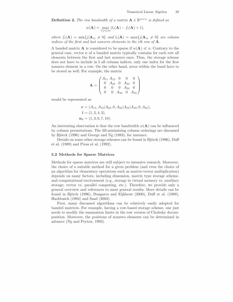
Definition 2. The row bandwidth of a matrix A ∈ Rm×n is defined as

w(A) = max1≤i≤m

(li(A) − fi(A) + 1),

where fi(A) = min{j|Aij �= 0} and li(A) = max{j|Aij �= 0} are columnindices of the first and last nonzero elements in the ith row of A.

A banded matrix A is considered to be sparse if w(A) � n. Contrary to thegeneral case, vector c of a banded matrix typically contains for each row allelements between the first and last nonzero ones. Thus, the storage schemedoes not have to include in i all column indices, only one index for the firstnonzero element in a row. On the other hand, zeros within the band have tobe stored as well. For example, the matrix

A =

A11 A12 0 0 00 A22 0 A24 00 0 0 A34 00 0 A43 0 A45

would be represented as

c = (A11, A12|A22, 0, A24|A34|A43, 0, A45),i = (1, 2, 4, 3),

n0 = (1, 3, 6, 7, 10).

An interesting observation is that the row bandwidth w(A) can be influencedby column permutations. The fill-minimizing column orderings are discussedby Bjorck (1996) and George and Ng (1983), for instance.

Details on some other storage schemes can be found in Bjorck (1996), Duffet al. (1989) and Press et al. (1992).

5.2 Methods for Sparse Matrices

Methods for sparse matrices are still subject to intensive research. Moreover,the choice of a suitable method for a given problem (and even the choice ofan algorithm for elementary operations such as matrix-vector multiplication)depends on many factors, including dimension, matrix type storage scheme,and computational environment (e.g., storage in virtual memory vs. auxiliarystorage; vector vs. parallel computing, etc.). Therefore, we provide only ageneral overview and references to most general results. More details can befound in Bjorck (1996), Dongarra and Eijkhout (2000), Duff et al. (1989),Hackbusch (1994) and Saad (2003).

First, many discussed algorithms can be relatively easily adopted forbanded matrices. For example, having a row-based storage scheme, one justneeds to modify the summation limits in the row version of Cholesky decom-position. Moreover, the positions of nonzero elements can be determined inadvance (Ng and Peyton, 1993).


Second, the algorithms for general sparse matrices are more complicated.A graph representation may be used to capture the nonzero pattern of amatrix as well as to predict the pattern of the result (e.g., the nonzero pat-tern of A�A, the Cholesky factor U, etc.). To give an overview, methodsadopted for sparse matrices include, but are not limited to, usually used de-compositions (e.g., Cholesky, Ng and Peyton, 1993; LU and LDU, Mittal andAl-Kurdi, 2002; QR, George and Liu, 1987, and Heath, 1984), solving sys-tems of equations by direct (Gupta, 2002; Tran et al., 1996) and iterativemethods (Makinson and Shah, 1986; Zlatev and Nielsen, 1988) and searchingeigenvalues (Bergamaschi and Putti, 2002; Golub et al., 2000).

References

Allanelli, M. and Hadjidimos, A. (2004). Block Gauss elimination followedby a classical iterative method for the solution of linear system. Journal ofComputational and Applied Mathematics : in press.

Anderson, E., Bai, Z., Bischof, C., Blackford, S., Demmel, J., Dongarra, J.,Croz, J.D., Greenbaum, A., Hammarling, S., McKenney, A. and Sorensen,D. (1999). LAPACK Users’ Guide, Third Edition. SIAM Press, Philadel-phia, USA.

Axelsson, O. (1994). Iterative Solution Methods. Cambridge University Press,Cambridge, UK.

Bergamaschi, L. and Putti, M. (2002). Numerical comparison of iterativeeigensolvers for large sparse symmetric positive definite matrices. ComputerMethods in Applied Mechanics and Engineering, 191: 5233–5247.

Benoit, C. (1924). Note sure une methode de resolution des equation mormalesprovenant de l’application de la methode des moindres carres a un systemee’equations lineaires en nombre inferieure a celuides inconnues. Applica-tion de la methode a la resolution d’un systeme defini d’equations lineaires(Procede du Commandant Cholesky). Bulletin geodesique, 24/2: 5–77.

Bjorck, A. (1994). Numerics of Gram-Schmidt Orthogonalization. Linear Al-gebra and Its Applications, 198: 297–316.

Bjorck, A. (1996). Numerical Methods for Least Squares Problems. SIAMPress, Philadelphia, USA.

Croz, J.D. and Higham, N.J. (1992). Stability of methods for matrix inversion.IMA Journal of Numerical Analysis, 12: 1–19.

Dax, A. (2000). A modified Gram-Schmidt algorithm with iterative orthogo-nalization and column pivoting. Linear Algebra and Its Applications, 310:25–42.

Demmel, J.W., Gu, M., Eisenstat, S., Slapnicar, I., Veselic, K. and Drmac,Z. (1999). Computing the singular value decomposition with high relativeaccuracy. Linear Algebra and its Applications, 299: 21–80.


Dongarra, J.J. and Eijkhout, V. (2000). Numerical linear algebra algorithmsand software. Journal of Computational and Applied Mathematics, 123:489–514.

Duff, I.S., Erisman, A.M. and Reid, J.K. (1989). Direct Methods for SparseMatrices. Oxford University Press, USA.

Freund, R. and Nachtigal, N. (1991). QMR: a quasi-minimal residual methodfor non-Hermitian linear systems. Numerical Mathematics, 60: 315–339.

Gallivan, K.A., Plemmons, R.J. and Sameh, A.H. (1990). Parallel algorithmsfor dense linear algebra computations. SIAM Review, 32: 54–135.

Gentle, J.E. (1998). Numerical Linear Algebra for Applications in Statistics.Springer, New York, USA.

Gentleman, W.M. (1973). Least squares computations by Givens transfor-mations without square roots. Journal of Institute of Mathematics and itsApplications, 12: 329–336,

Gentleman, W.M. (1975). Error analysis of QR decomposition by Givenstransformations. Linear Algebra and its Applications, 10: 189–197.

George, A. and Liu, J.W.H. (1987). Householder reflections versus givens ro-tations in sparse orthogonal decomposition. Linear Algebra and its Appli-cations, 88: 223–238.

George, J.A. and Ng, E.G. (1983). On row and column orderings for sparseleast squares problems. SIAM Journal of Numerical Analysis, 20: 326–344.

Givens, W. (1958). Computation of Plane Unitary Rotations Transforming aGeneral Matrix to Triangular Form. Journal of SIAM, 6/1: 26–50.

Golub, G.H. (1965). Numerical methods for solving least squares problems.Numerical Mathematics, 7: 206–216.

Golub, G.H. and Kahan, W. (1965). Calculating the singular values andpseudo-inverse of a matrix. SIAM Journal on Numerical Analysis B, 2:205–224.

Golub, G.H. and Reinsch, C. (1970). Singular value decomposition and leastsquares solution. Numerical Mathematics, 14: 403–420.

Golub, G.H. and van Loan, C.F. (1996). Matrix Computations. Johns HopkinsUniversity Press, Baltimore, Maryland.

Golub, G.H., Zhang, Z. and Zha, H. (2000). Large sparse symmetric eigenvalueproblems with homogeneous linear constraints: the Lanczos process withinner-outer iterations. Linear Algebra and its Applications, 309: 289–306.

Gupta, A. (2002). Recent Advances in Direct Methods for Solving Unsym-metric Sparse Systems of Linear Equations. ACM Transactions on Mathe-matical Software, 28: 301–324.

Hackbusch, W. (1994). Iterative Solution of Large Sparse Systems of Equa-tions. Springer, New York, USA.

Hadjidimos, A. (2000). Successive Overrelaxation (SOR) and related methods.Journal of Computational and Applied Mathematics, 123: 177–199.

Hammarling, S. (1974). A note on modifications to the Givens plane rotation.Journal of Institute of Mathematics and its Applications, 13: 215–218.


Hari, V. and Veselic, K. (1987). On Jacobi methods for singular value decom-positions. SIAM Journal of Scientific and Statistical Computing, 8: 741–754.

Harville, D.A. (1997). Matrix Algebra from a Statistician’s Perspective.Springer, New York, USA.

Heath, M.T. (1984). Numerical methods for large sparse linear least squaresproblems. SIAM Journal of Scientific and Statistical Computing, 26: 497–513.

Hestenes, M.R. and Stiefel, E. (1952). Method of conjugate gradients for solv-ing linear systems. J. Res. Nat Bur. Standards B, 49: 409–436.

Higham, N.J. (1989). The accuracy of solutions to triangular systems. SIAMJournal on Numerical Analysis, 26: 1252–1265.

Higham, N.J. (1997). Recent Developments in Dense Numerical Linear Alge-bra. In Duff, I.S. and Watson, G.A. (eds), State of the Art in NumericalAnalysis, Oxford University Press, Oxford.

Higham, N.J. (2000). QR factorization with complete pivoting and accuratecomputation of the SVD. Linear Algebra and its Applications, 309: 153–174.

Higham, N.J. (2002). Accuracy and Stability of Numerical Algorithms, Secondedition. SIAM Press, Philadelphia, USA.

Hong, Y.P. and Tan, C.T. (1992). Rank-revealing QR fatorizations and thesingular value decomposition. Mathematics of Computation, 58: 213–232.

Householder, A.S. (1958). Unitary triangularization of a nonsymmetric ma-trix. Journal of the Association of Computing Machinery, 5: 339–342.

Ipsen, I.C.F. (1997). Computing an Eigenvector with Inverse Iteration. SIAMReview, 39: 254–291.

Kahan, W. (1958). Gauss-Seidel methods of solving large systems of linearequations. Doctoral thesis, University of Toronto, Toronto, Canada.

Kammerer, W.J. and Nashed, M.Z. (1972). On the convergence of the conju-gate gradient method for singular linear operator equations. SIAM Journalon Numerical Analysis, 9: 165–181.

Makinson, G.J. and Shah, A.A. (1986). An iterative solution method for solv-ing sparse nonsymmetric linear systems. Journal of Computational and Ap-plied Mathematics, 15: 339–352.

Martin, R.S., Peters, G. and Wilkinson, J.H. (1965). Symmetric decomposi-tion of a positive definite matrix. In Wilkinson, J.H. and Reinsch, C. (eds),Linear Algebra (Handbook for Automation Computation, Vol. II). Springer,Heidelberg, Germany.

Meinguet, J. (1983). Refined error analysis of cholesky factorization. SIAMJournal on Numerical Analysis, 20: 1243–1250.

Milaszewicz, J.P. (1987). Improving Jacobi and Gauss-Seidel Iterations. Lin-ear Algebra and Its Applications, 93: 161–170.

Miranian, L. and Gu, M. (2003). Strong rank revealing LU factorizations.Linear Algebra and its Applications, 367: 1–16.

Mittal, R.C. and Al-Kurdi, A. (2002). LU-decomposition and numerical struc-ture for solving large sparse nonsymmetric linear systems. Computers &Mathematics with Applications, 43: 131–155.


Ng, E.G. and Peyton, B.W. (1993). Block Sparse Cholesky Algorithm onAdvanced Uniprocessor Computers. SIAM Journal of Scientific Computing,14: 1034–1056.

Nool, M. (1995). Explicit parallel block Cholesky algorithms on the CRAYAPP. Applied Numerical Mathematics, 19: 91-114.

Pan, C.T. (2000). On the existence and computation of rank revealing LUfactorizations. Linear Algebra and its Applications, 316: 199–222.

Press, W.H., Teukolsky, S.A., Vetterling, W.T. and Flannery, B.P. (1992).Numerical Recipes in C: the Art of Scientific Computing, Second Edition.Cambridge University Press, Cambridge, UK.

Rice, J.R. (1966). Experiments on Gram-Schmidt orthogonalization. Mathe-matics of Computation, 20: 325–328.

Saad, Y. (2003). Iterative Methods for Sparse Linear Systems. Second Edition.SIAM Press, USA.

Saad, Y. and Schultz, M.H. (1986). GMRES: a generalized minimal resid-ual algorithm for solving nonsymmetric linear systems. SIAM Journal ofScientific and Statistical Computing, 7: 856–869.

Sidi, A. (1989). On extensions of the power method for normal operators.Linear Algebra and Its Applications, 120: 207–224.

Skeel, R.D. (1980). Iterative refinement implies numerical stability for Gaus-sian elimination. Mathematics of Computation, 35: 817–832.

Stewart, G.W. (1976). The economical storage of plane rotations. NumericalMathematics, 25: 137–138.

Stewart, G.W. (1998). Matrix Algorithms, Volume I: Basic Decompositions.SIAM Press, Philadelphia, USA.

Stoer, J. and Bulirsch, R. (2002). Introduction to Numerical Analysis, ThirdEdition. Springer, New York, USA.

Tran, T.M., Gruber, R., Appert, K. and Wuthrich, S. (1996). A direct parallelsparse matrix solver. Computer Physics Communications, 96: 118–128.

Trefethen, L.N. and Bau, D. (1997). Numerical Linear Algebra. SIAM Press,Philadelphia, USA.

von Matt, U. (1995). The Orthogonal QD-Algorithm. In Moonen, M. and DeMoor, B. (eds), SVD and Signal Processing, III: Algorithms, Architecturesand Applications, Elsevier, Amsterdam.

Vorst, V.D. (1992). Bi-CGSTAB: A fast and smoothly converging variant ofBi-CG for the solution of nonsymmetric linear systems. SIAM Journal ofScientific and Statistical Computing, 13: 631–644.

Wampler, R.H. (1970). A report on the accuracy of some widely used leastsquares computer programs. Journal of American Statistical Association,65: 549–565.

Young, D.M. (1954). Iterative methods for solving partial differential equa-tions of elliptic type. Transactions of the American Mathematical Society,76: 92–111.


Zhou, B.B. and Brent, R.P. (2003). An efficient method for computing eigen-values of a real normal matrix. Journal of Parallel and Distributed Com-puting, 63: 638–648.

Zlatev, Z. and Nielsen, H.B. (1988). Solving large and sparse linear least-squares problems by conjugate gradient algorithms. Computers & Mathe-matics with Applications, 15: 185–202.

Zou, Q. (1991). An observation on Gauss elimination. Computers and Math-ematical Applications, 22: 69–70.

Index

Cholesky decomposition, 2conjugate gradient method, 23

eigenvalues, 23inverse iterations, 27Jacobi method, 25LR method, 26power method, 24QR method, 26

eigenvectors, 23

Gauss-Jordan elimination, 14Gauss-Seidel method, 20, 22Givens rotations, 7Gram-Schmidt orthogonalization, 10

Householder reflections, 6

inverse iterations, 27iterative refinement, 16

Jacobi method, 19, 25

linear systemdirect methods, 13

Gauss-Jordan elimination, 14iterative refinement, 16

gradient methods, 22conjugate gradient method, 23Gauss-Seidel method, 22steepest descent method, 22

iterative methods, 17Gauss-Seidel method, 20general principle, 17Jacobi method, 19SOR method, 21

LR method, 26LU decomposition, 4

matrix decompositions, 2Cholesky decomposition, 2Givens rotations, 7Gram-Schmidt orthogonalization, 10Householder reflections, 6LU decomposition, 4QR decomposition, 5SVD decomposition, 11

matrix inversion, 12

power method, 24

QR decomposition, 5QR method, 26

SOR method, 21sparse matrices, 27steepest descent method, 22SVD decomposition, 11systems of linear equations

direct methods, 13Gauss-Jordan elimination, 14iterative refinement, 16

gradient methods, 22conjugate gradient method, 23Gauss-Seidel method, 22steepest descent method, 22

iterative methods, 17Gauss-Seidel method, 20general principle, 17Jacobi method, 19SOR method, 21

Date post:	20-Mar-2020
Category:	Documents
Upload:	others
View:	9 times
Download:	0 times

Numerical Linear Algebra - EconStor · 2020-01-16 · Numerical Linear Algebra 3 Theorem 1. Let...

Documents