Numerical Methods and Simulation Techniques for ﬂow with ... fileNumerical Methods and Simulation...

Numerical Methods and Simulation Techniquesfor flow with Shear and Pressure dependent

Viscosity

Abderrahim Ouazzi, Stefan Turek

Institute for Applied Mathematics, LS III,

Dortmund University,

Germany

Numerical Methods and Simulation Techniques for flow with Shear and Pressure dependent Viscosity – p. 1/19

Motivation of this work

The flow of granular materials

Example of applicationPharmaceutical Industry, Food Processing, Soil Mechanics ...

Granular material storage Couette flow

What about the viscosity !!?

From engineering point of view this material does not have anyviscosity!!

From mathematical and numerical point of view we are able to setthis type of fluid in the same range of flow with generalizedviscosity, since it exibits the same difficulties !?


Equations of motion

The general equation of motion for incompressible powders

Conservation of mass

DρDt

= ∂ρ∂t

+ ∇ · (ρu) = 0

D∗Dt

is the material derivative and u is the velocity vector

For an incompressible materialthe bulk density, ρ, is a constant thus

∇ · u = 0

The equation of motion

ρDuDt

= −∇ · T + ρg

with, T = S + pI, the deviatoric stress.


Constitutive equation

The constitutive equation is devoted to correlate between the deviatorictensor, S, and the velocity, throught the rate of deformationD = −1

2(∇u + ∇T u) , and assure the closure of equations.

Newtonian lawS = 2νoD

Power lawS = 2ν(DII)D, ν(z) = z

r2−1, r > 1

Schaeffer’s law (1987): For a powder a constitutive equation firstintroduced by Schaeffer (1997), which has to obey a

yield condition; ||S|| =√

2p sinφ, and

flow rule; S = λD

we use this correlation to obtain the constitutive equation

S =√

2p sinφ D

||D||


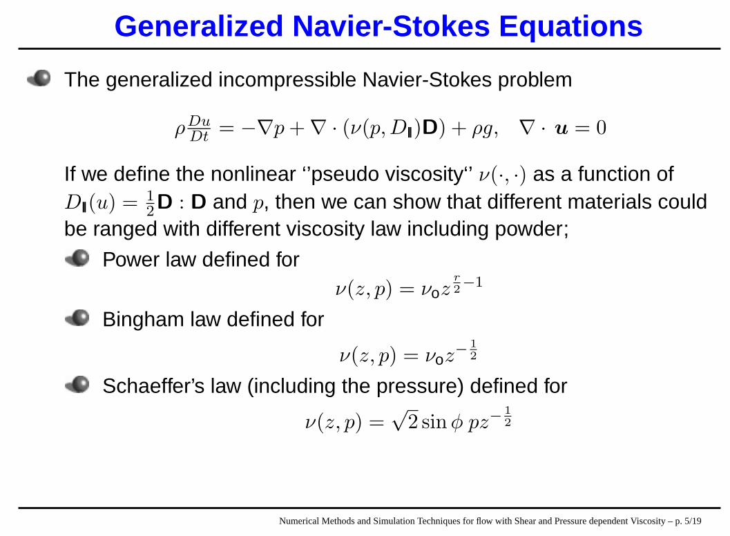
Generalized Navier-Stokes Equations

The generalized incompressible Navier-Stokes problem

ρDuDt

= −∇p + ∇ · (ν(p, DII)D) + ρg, ∇ · u = 0

If we define the nonlinear ‘’pseudo viscosity‘’ ν(·, ·) as a function ofDII(u) = 1

2D : D and p, then we can show that different materials couldbe ranged with different viscosity law including powder;

Power law defined forν(z, p) = νoz

r2−1

Bingham law defined for

ν(z, p) = νoz− 1

2

Schaeffer’s law (including the pressure) defined for

ν(z, p) =√

2 sin φ pz−1

2


New problems

In what follows we will show how to deal with the following problems

Discretization method:How to use nonconforming finite element methods for problemsinvolving rate of deformation tensor rather than the gradient !?

Nonlinear solver:How to apply Newton linearization technique for this highly nonlinearand irregular problem !?

Linear multigrid solver:In connection with the first two problems, how to keep the efficiency ofthe linear multigrid solver!?


Nonlinear Solver: Newton iteration

Let ul being the initial state, the (continuous) Newton method consists offinding u such that

∫

Ω2ν(DII(u

l), pl)D(u) : D(v)dx

+

∫

Ω2∂1ν(DII(u

l), pl)[D(ul) : D(u)][D(ul) : D(v)]dx

+

∫

Ω2∂2ν(DII(u

l), pl)[D(ul) : D(v)]pdx

=

∫

Ωfv −

∫

Ω2ν(DII(u

l), pl)D(ul) : D(v)dx, ∀v, (1)

where ∂iν(·, ·); i = 1, 2 is the partial derivative of ν related to the first andsecond variable, respectively.


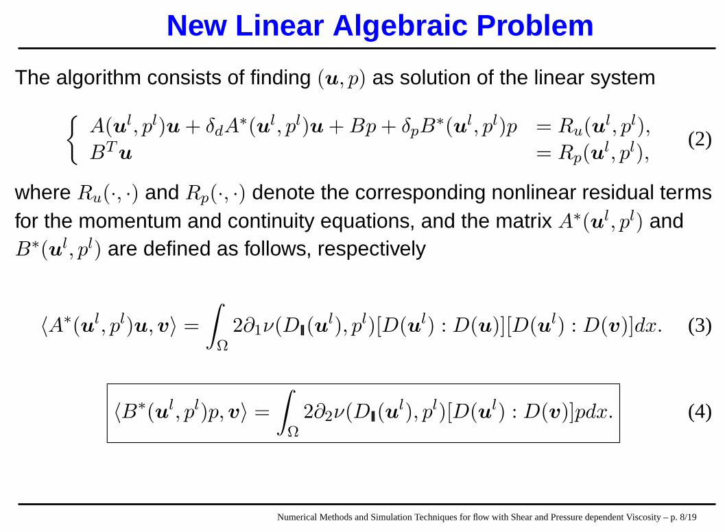
New Linear Algebraic Problem

The algorithm consists of finding (u, p) as solution of the linear system

A(ul, pl)u + δdA∗(ul, pl)u + Bp + δpB

∗(ul, pl)p = Ru(ul, pl),

BT u = Rp(ul, pl),

(2)

where Ru(·, ·) and Rp(·, ·) denote the corresponding nonlinear residual termsfor the momentum and continuity equations, and the matrix A∗(ul, pl) andB∗(ul, pl) are defined as follows, respectively

〈A∗(ul, pl)u,v〉 =

∫

Ω2∂1ν(DII(u

l), pl)[D(ul) : D(u)][D(ul) : D(v)]dx. (3)

〈B∗(ul, pl)p,v〉 =

∫

Ω2∂2ν(DII(u

l), pl)[D(ul) : D(v)]pdx. (4)


Spatial discretization

Quadrilateral Rannacher-Turek Stokes Element

P1

P2

P3P4

M1

M2

M3

M4M

E2E1

Advantage:

Stable and efficient for incompressible flow.

Compact data structures.

Disadvantage:Not satisfying discrete Korn’s inequality

∑

τ∈τh

‖v‖H1(τ) ≤ c(‖v‖2L2 + ‖D(v)‖2

L2)1

2 (5)


Kernel function

The specific kernel function takes -1 or 1 in midpoints

The constants in Korn’s inequality for gradient, tensor and thestabilized tensor

NEL ‖uh‖G ‖uh‖T ‖uh‖ST

256 1.3 6.9 × 10−13

0.85

1024 1.4 1.4 × 10−13

0.90

4096 1.4 3.0 × 10−12

0.92

16384 1.4 6.1 × 10−12

0.93


Stabilized Rannacher-Turek Stokes Element

Remedy: Stabilized R-T FEM (Hansbo et. al)

The stabilization consists of adding the following bilinear form

∑

E∈EI∪ED

1

|E|

∫

E

[φi][φj ]ds (6)

for all basis function φi and φj with a weighted parameter s = s(ν), then thecorresponding matrix S is defined as:

< Su, v >=∑

E∈EI∪ED

1

|E|

∫

E

[u][v]ds (7)


Linear solverMultigrid for velocity and pressure simultanously:

Vanca-like block Gauss-Seidel scheme as smoother and solveradaptive step length control for correction step (with F-cycle)

macro-elementwise interpolation for grid-transfer

Reduced sparsity of the matrix S

Edge

Defect correction method:[

ul+1

pl+1

]

=

[

ul

pl

]

+ ωl∑

i

(

F + S∗|Ωi

B + δpB∗|Ωi

BT|Ωi

0

)−1[

Ru(ul, pl)

Rp(ul, pl)

]

For the preconditioning step only a part of the matrix, i.e. F + S∗, is taken


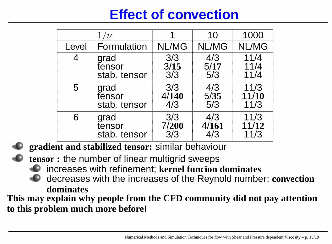
Newtonian caseIn this case the gradient and tensor formulation are equivalent; the efficiencyof the stabilized tensor discretization is checked by comparison with thegradient one on the flow around cylinder benchmark

Level 51/ν grad tensor stab. tensor

1 Drag 31252 × 10−1 31221 × 10−1 31231 × 10−1

Lift 30898 × 10−3 30924 × 10−3 30936 × 10−3

1000 Drag 55657 × 10−4 55531 × 10−4 55535 × 10−4

(Re = 20) Lift 10180 × 10−6 10259 × 10−6 10277 × 10−6

For all three formulations the lift and drag forces are similar


Power law case

In this case the nonlinear viscosity has the form ν(z) = νozr2−1, z = DII, the

gradient and tensor formulation are not equivalent any more. The quality ofthe solution is checked by the comparison with the stable conforming Q2/P1

approximation,

Level Elements Drag Lift p Drag Lift p

Power r = 1.5 r = 1.1

4 Q1/Q0 1594.20 14.25 24.56 916.02 3.7381 15.74

Q2/P1 1635.80 14.39 25.09 953.94 3.9217 15.82

5 Q1/Q0 1615.60 14.43 24.81 935.13 3.9954 15.82

Q2/P1 1637.60 14.44 25.07 957.64 4.0587 15.87

6 Q1/Q0 1626.20 14.46 24.94 946.22 4.0592 15.85

The accuracy of the FEM is saved with stabilized tensor discretization!


Effect of convection1/ν 1 10 1000

Level Formulation NL/MG NL/MG NL/MG4 grad 3/3 4/3 11/4

tensor 3/15 5/17 11/4stab. tensor 3/3 5/3 11/4

5 grad 3/3 4/3 11/3tensor 4/140 5/35 11/10stab. tensor 4/3 5/3 11/3

6 grad 3/3 4/3 11/3tensor 7/200 4/161 11/12stab. tensor 3/3 4/3 11/3

gradient and stabilized tensor:similar behaviourtensor : the number of linear multigrid sweeps

increases with refinement; kernel funcion dominatesdecreases with the increases of the Reynold number; convectiondominates

This may explain why people from the CFD community did not pay attentionto this problem much more before!


Pressure dependent viscosityIn this case the nonlinear pseudo viscosity has the form ν(p, z) = Q(p)z

r2−1

The corresponding matrix of the linear problem

can no longer be fitted into classical saddle point problems;

Mδp(u, p) =

(

A B + δpB∗

BT 0

)

the solution is relative to the choice of imposing the uniqueness,since dim(null(Mδp

)) = 1

Efficiency of the solver:we increase the nonlinearity and list the numberof resulting nonlinear iterations and the averaged number of multigridsweeps per nonlinear iteration for both Newton and fixpoint

ν(z, p) = exp(βp) Fixpoint NewtonLevel β 0.1 0.3 0.5 0.1 0.3 0.5

5 stab. tensor 6/2 12/2 33/2 3/3 4/2 4/3

gradient 6/2 11/2 34/2 3/3 4/2 4/3

6 stab. tensor 5/3 11/3 65/2 3/3 3/3 3/3gradient 5/3 9/3 76/2 3/3 3/3 5/3


Schaeffer’s law

Schaeffer’s law:The time dependent equations are linearly ill-posedaccording to Schaeffer; in the Navier-Stokes equations, the pressureforce associated to the constraint div v = 0 can do no work. Bycontrast, the pressure force in equation of granular flow can do work,and for plane waves in certain directions, it does so.

Pseudo compressibility:This scheme is an effort to regularize theinstability in order to study the shear-band

average stress shear stress

t1 t2 t3 t1 t2 t3

The plot of the average stress and shear stress in a hopper shows thedevelopment of instability which leads to shear-banding.


OutlookWe have been able to develop the numerical methods and techniques tosimulate a dense granular flow, in futur we want to cover a wide range ofgranular materials

General equation of motion for a powder

ρDu

Dt= −∇p + ∇ ·

[

q(p,ρ)

||D− 1

n∇·uI||

(

D − 1n∇ · uI

)

]

+ ρg, with

Continuity equation∂ρ∂t

+ ∇ · (ρu) = 0, and

Normality condition∇ · u = ∂q(p,ρ)

∂p

∣

∣

∣

∣D − 1n∇ · uI

∣

∣

∣

∣

the yield condition q(p, ρ) is given by:

Powder properties Non-cohesive CohesiveIncompressible p sinφ p sinφ + c cos φ

Compressible p sinφ

[

2 − p

ρ1

β

]

p sinφρ1

β − C (p−ρ1

β )2

ρ1

β


Date post:	08-Aug-2019
Category:	Documents
Upload:	lynhu
View:	234 times
Download:	0 times

Numerical Methods and Simulation Techniques for ﬂow with ... fileNumerical Methods and Simulation...

Documents