NUMERICAL METHODS CONTENTS - Orange -...

BSc Computing Mathematics BSc Computing Maths with Business Studies

Year 2

MATHEMATICAL TECHNIQUES:

NUMERICAL METHODS

CONTENTS

TOPIC Page Interpolation 4 Difference Tables 6 Newton-Gregory Forward Interpolation Formula 8 Newton-Gregory Backward Interpolation Formula 13 Central Differences 16 Numerical Differentiation 21 Numerical Solution of Differential Equations 26 Euler's Method 26 Improved Euler Method (IEM) 33 Runge-Kutta Method 39

NUMERICAL ANALYSIS When handling problems using mathematical techniques it is usually necessary to establish a model, and to write down equations expressing the constraints and physical laws that apply. These equations must now be solved and a choice presents itself. One way is to proceed using conventional methods of mathematics, obtaining a solution in the form of a formula, or set of formulae. Another method is to express the equations in such a way that they may be solved computationally, ie by using methods of numerical analysis. This will lead directly to quantitative results, however if enough such results are obtained then qualitative results may emerge. Using these methods, large and complex physical systems may be modelled, and otherwise intractable problems can be solved with the help of modern computer systems. Interpolation We sometimes know the value of a function f(x) at a set of points, without knowing the analytic expression for f(x) that would allow us to calculate its value at some arbitrary point. Often the points at which we know the value of f(x) are equally spaced, but not always. The task is to estimate f(x) for a given value of x by, in some sense, drawing a smooth curve through (and perhaps beyond) the known values. If the desired value is in between the smallest and largest x-values already know, then the process is called interpolation. If x is outside that range, it is called extrapolation, which is considerably more hazardous. As a simple illustration, let us consider linear interpolation. Before the advent of computers, if it was required, for example, to find the square root of a number x, a table of such numbers was consulted. If the number did not appear in the table, then the two numbers above and below x were used, and interpolation provided the solution. For example, suppose we wanted the square root of 2.155 and had a table such as shown below:

n n 2.140 1.46287 2.150 1.46629 2.160 1.46969 2.170 1.47309

The difference between the square roots of 2.15 and 2.16 is 0.0034. Since 2.155 is half-way between 2.15 and 2.16 we could assume that its square root was half-way between the square roots of 2.15 and 2.16. This gives 2.155 = 1.46799. Had we wanted 2.153 we would have added 0.3 times 0.0034 to 2.15. This is the process of LINEAR INTERPOLATION, in which we assume a linear variation between the two known values to predict intermediate values. Suppose we have a set of m numbers x x x xm1 2 3, , ,... , and that corresponding to each xi there is a yi , where y and x are related by some function f: y f x= ( ). If we are given a value of x (not equal to one of the xi ) we want to find a value of y obtained by linear interpolation. Naturally we assume some functional relationship does indeed exist between x and y, and it is our responsibility to ensure that this is a valid assumption. Suppose that the required value of the variable x falls between the kth and k+1th known values of x [we assume that the x's are ordered in an ascending sequence so that x x x xm1 2 3< < < <... ]

∴ ≤ ≤ +x x xk k 1

BSc 2 Computing Mathematics / Computing Maths with Business Studies - Mathematical Techniques

4

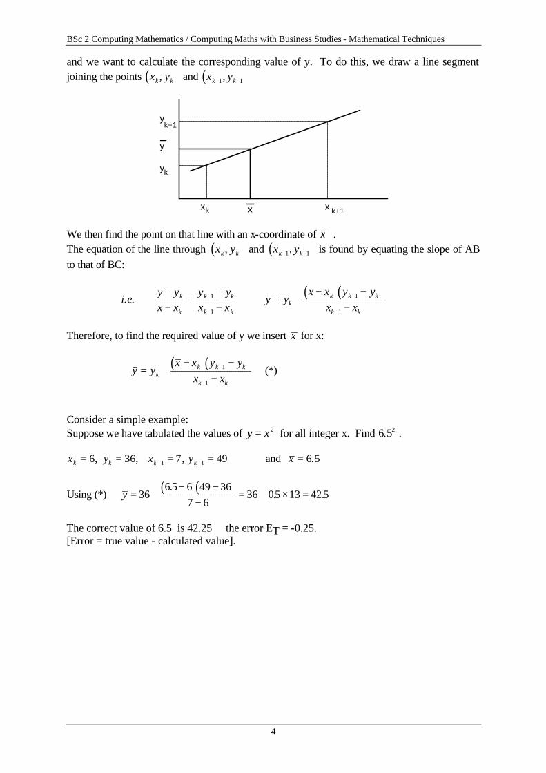
and we want to calculate the corresponding value of y. To do this, we draw a line segment joining the points ( )x yk k, and ( )x yk k+ +1 1,

x x x

y

y

yk

k+1

k k+1 We then find the point on that line with an x-coordinate of x . The equation of the line through ( )x yk k, and ( )x yk k+ +1 1, is found by equating the slope of AB to that of BC:

( )( )i ey yx x

y yx x

y yx x y y

x xk

k

k k

k kk

k k k

k k

. .−−

=−−

∴ = +− −

−+

+

+

+

1

1

1

1

Therefore, to find the required value of y we insert x for x:

( )( )∴ = +− −

−+

+

y yx x y y

x xkk k k

k k

1

1

(*)

Consider a simple example: Suppose we have tabulated the values of y x= 2 for all integer x. Find 6 52. . x y x y xk k k k= = = = =+ +6 36 7 49 6 51 1, , , .and

Using (*) ( )( )y = +− −

−= + × =36

6 5 6 49 367 6

36 05 13 42 5.

. .

The correct value of 6.5 is 42.25 the error ET = -0.25. [Error = true value - calculated value].


5

A General Approach to Interpolation We could investigate methods of interpolation using higher order polynomials, but although quadratic interpolation, for example, is likely to be more accurate than linear interpolation, it is by no means certain to provide sufficient accuracy all the time. We need to develop a general method which will also enable extra accuracy to be attained without having to resort to a new set of calculations. In order to do this we need to introduce the idea of a difference table. Difference Table As before, suppose that we have a set of values of an unknown function y y y yn1 2 3, , ,..., corresponding to a set of values of the (known) independent variable x x x xn1 2 3, , ,..., where x x x xn1 2 3< < < <... . A reliable formula for interpolation, to obtain the value of y corresponding to any x (where x x x xn1 2 3< < < <... ) will employ all the given information - ie it will be based on the values of the n+1 data entries. Instead of using these directly it is more convenient to use relationships dependent on these values. The relationship y yr r+ −1 is called the first difference of yr , denoted by ∆yr : ∆y y yr r r= −+1 Similarly, the relationship ∆ ∆y yr r+ −1 is the second difference: ∆ ∆ ∆2

1y y yr r r= −+ For example, ( ) ( )∆ ∆ ∆2

0 1 0 2 1 1 0 2 1 02y y y y y y y y y y= − = − − − = − + Similarly ( ) ( )∆ ∆ ∆2

1 2 1 3 2 2 1 3 2 12y y y y y y y y y y= − = − − − = − + In general terms: ∆2

2 12 0 1 2 2y y y y r nr r r r= − + = −+ + , , ,... , The third differences are ∆3

3 2 13 3 0 1 2 3y y y y y r nr r r r r= − + − = −+ + + , , , ...,


6

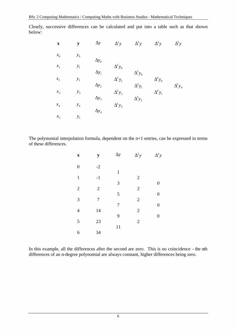
Clearly, successive differences can be calculated and put into a table such as that shown below:

x y ∆y ∆2 y ∆3 y ∆4 y ∆5y

x0 y0 ∆y0

x1 y1 ∆20y

∆y1 ∆30y

x2 y2 ∆21y ∆4

0y ∆y2 ∆3

1y ∆50y

x3 y3 ∆22y ∆4

1y ∆y3 ∆3

2y x4 y4 ∆2

3y ∆y4

x5 y5 The polynomial interpolation formula, dependent on the n+1 entries, can be expressed in terms of these differences.

x y ∆y ∆2 y ∆3 y

0 -2 1

1 -1 2 3 0

2 2 2 5 0

3 7 2 7 0

4 14 2 9 0

5 23 2 11

6 34 In this example, all the differences after the second are zero. This is no coincidence - the nth differences of an n-degree polynomial are always constant, higher differences being zero.


7

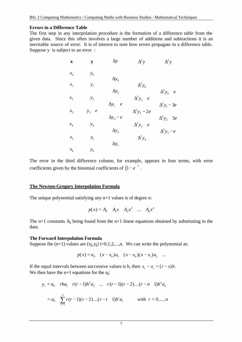
Errors in a Difference Table The first step in any interpolation procedure is the formation of a difference table from the given data. Since this often involves a large number of additions and subtractions it is an inevitable source of error. It is of interest to note how errors propagate in a difference table. Suppose y is subject to an error :

x y ∆y ∆2 y ∆3 y

x0 y0 ∆y0

x1 y1 ∆20y

∆y1 ∆30y + ε

x2 y2 ∆21y + ε

∆y2 + ε ∆31 3y − ε

x3 y3 + ε ∆22 2y − ε

∆y3 − ε ∆32 3y + ε

x4 y4 ∆23y + ε

∆y4 ∆33y − ε

x5 y5 ∆24y

∆y5 x6 y6

The error in the third difference column, for example, appears in four terms, with error coefficients given by the binomial coefficients of ( )1 3− ε . The Newton-Gregory Interpolation Formula The unique polynomial satisfying any n+1 values is of degree n:

p x A A x A x A xnn( ) ...= + + + +0 1 2

2

The n+1 constants Ai being found from the n+1 linear equations obtained by substituting in the data. The Forward Interpolation Formula Suppose the (n+1) values are (xi,yi) i=0,1,2,...,n. We can write the polynomial as:

p x a x x a x x x x a( ) ( ) ( )( ) ...= + − + − − +0 0 1 0 1 2 If the equal intervals between successive values is h, then x x r s hr s− = −( ) . We then have the n+1 equations for the ai: y a rha r r h a r r r r n h ar

nn= + + − + + − − − +0 1

221 1 2 1( ) ... ( )( )...( )

= + − − − + ==

∑a r r r r t h a r nt

t

n

t01

1 2 1 0( )( ) ...( ) ,...,with


8

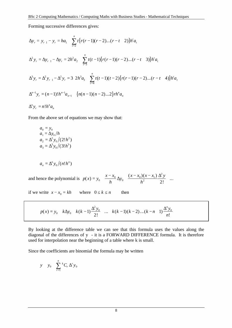
Forming successive differences gives:

{ }∆y y y ha t r r r r t h ar r rt

nt

t= − = + − − − ++=∑1 1

2

1 2 2( )( )...( )

{ }∆ ∆ ∆21

22

3

2 1 1 2 3y y y h a t t r r r r t h ar r rt

nt

t= − = + − − − − ++=∑ ( ) ( )( )...( )

{ }∆ ∆ ∆3 21

2 33

4

3 2 1 2 1 2 4y y y h a t t t r r r r t h ar r rt

nt

t= − = ⋅ + − − − − − ++=∑ ( )( ) ( )( )...( )

{ }∆n

rn

nn

ny n h a n n n rh a− −−= − + − −1 1

11 1 2 2( )! ( )( )... ∆n

rn

ny n h a= ! From the above set of equations we may show that: a y0 0= a y h1 0= ∆ a y h2

20

22= ∆ ( ! ) a y h3

30

33= ∆ ( ! ) ⋅ ⋅ a y n hn

n n= ∆ 0 ( ! )

and hence the polynomial is p x yx x

hy

x x x xh

y( )

( )( )!

...= +−

+− −

+00

00 1

2

2

2∆

∆

if we write x x kh k n− = ≤ ≤0 0where then

p x y k y k ky

k k k k ny

n

n

( ) ( )!

... ( )( ) ... ( )!

= + + − + + − − − +0 0

20 01

21 2 1∆

∆ ∆

By looking at the difference table we can see that this formula uses the values along the diagonal of the differences of y - it is a FORWARD DIFFERENCE formula. It is therefore used for interpolation near the beginning of a table where k is small. Since the coefficients are binomial the formula may be written

y y C yk

r

n

rr≅ +

=∑0

10∆


9

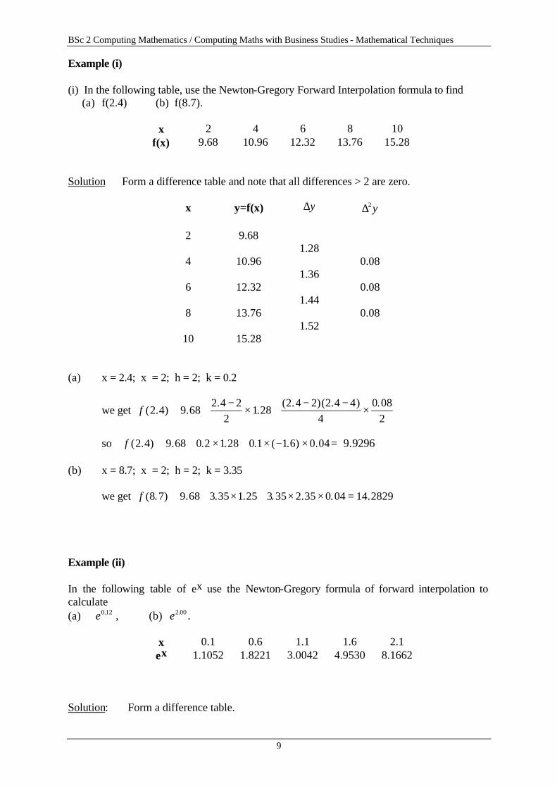
Example (i) (i) In the following table, use the Newton-Gregory Forward Interpolation formula to find (a) f(2.4) (b) f(8.7).

x 2 4 6 8 10 f(x) 9.68 10.96 12.32 13.76 15.28

Solution Form a difference table and note that all differences > 2 are zero.

x y=f(x) ∆y ∆2 y

2 9.68 1.28 4 10.96 0.08 1.36 6 12.32 0.08 1.44 8 13.76 0.08 1.52

10 15.28 (a) x = 2.4; x = 2; h = 2; k = 0.2

we get f ( . ) ..

.( . )( . ) .

2 4 9 682 4 2

21 28

2 4 2 2 4 44

0 082

≅ +−

× +− −

×

so f ( . ) . . . . ( . ) .2 4 9 68 0 2 1 28 0 1 1 6 0 04≅ + × + × − × = 9 9296. (b) x = 8.7; x = 2; h = 2; k = 3.35 we get f ( . ) . . . . . . .8 7 9 68 3 35 1 25 3 35 2 35 0 04 14 2829≅ + × + × × = Example (ii) In the following table of ex use the Newton-Gregory formula of forward interpolation to calculate (a) e0 12. , (b) e2 00. .

x 0.1 0.6 1.1 1.6 2.1 ex 1.1052 1.8221 3.0042 4.9530 8.1662

Solution: Form a difference table.


10

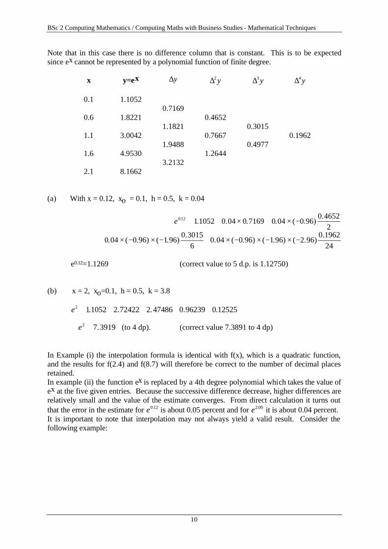
Note that in this case there is no difference column that is constant. This is to be expected since ex cannot be represented by a polynomial function of finite degree.

x y=ex ∆y ∆2 y ∆3 y ∆4 y

0.1 1.1052 0.7169

0.6 1.8221 0.4652 1.1821 0.3015

1.1 3.0042 0.7667 0.1962 1.9488 0.4977

1.6 4.9530 1.2644 3.2132

2.1 8.1662 (a) With x = 0.12, xo = 0.1, h = 0.5, k = 0.04

∴ ≅ + × + × −e012 1 1052 0 04 0 7169 0 04 0 960 4652

2. . . . . ( . )

.

+ × − × − + × − × − × −0 04 0 96 1 960 3015

60 04 0 96 1 96 2 96

0 196224

. ( . ) ( . ).

. ( . ) ( . ) ( . ).

∴ e0.12=1.1269 (correct value to 5 d.p. is 1.12750) (b) x = 2, xo=0.1, h = 0.5, k = 3.8 e2 1 1052 2 72422 2 47486 0 96239 0 12525≅ + + + +. . . . . ∴ ≅e2 7 3919. (to 4 dp). (correct value 7.3891 to 4 dp) In Example (i) the interpolation formula is identical with f(x), which is a quadratic function, and the results for f(2.4) and f(8.7) will therefore be correct to the number of decimal places retained. In example (ii) the function ex is replaced by a 4th degree polynomial which takes the value of ex at the five given entries. Because the successive difference decrease, higher differences are relatively small and the value of the estimate converges. From direct calculation it turns out that the error in the estimate for e0 12. is about 0.05 percent and for e2 00. it is about 0.04 percent. It is important to note that interpolation may not always yield a valid result. Consider the following example:


11

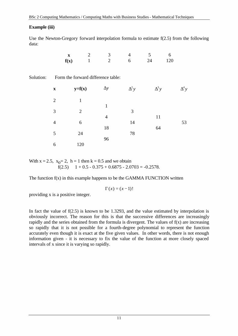
Example (iii) Use the Newton-Gregory forward interpolation formula to estimate f(2.5) from the following data:

x 2 3 4 5 6 f(x) 1 2 6 24 120

Solution: Form the forward difference table:

x y=f(x) ∆y ∆2 y ∆3 y ∆4 y 2 1 1 3 2 3 4 11

4 6 14 53 18 64

5 24 78 96 6 120

With x = 2.5, xo= 2, h = 1 then k = 0.5 and we obtain f(2.5) ≅ 1 + 0.5 - 0.375 + 0.6875 - 2.0703 = -0.2578. The function f(x) in this example happens to be the GAMMA FUNCTION written

Γ ( ) ( )!x x= −1 providing x is a positive integer. In fact the value of f(2.5) is known to be 1.3293, and the value estimated by interpolation is obviously incorrect. The reason for this is that the successive differences are increasingly rapidly and the series obtained from the formula is divergent. The values of f(x) are increasing so rapidly that it is not possible for a fourth-degree polynomial to represent the function accurately even though it is exact at the five given values. In other words, there is not enough information given - it is necessary to fix the value of the function at more closely spaced intervals of x since it is varying so rapidly.


12

The Newton-Gregory Backward Interpolation Formula The formula derived in the previous section is appropriate when the required value (xo,yo) lies near the beginning of the tabulated data. When (xo,yo) is near the end of the table, it is necessary to find a polynomial satisfying the (n+1) values (x-i,y-i), i=0,1,2,...,n. This may be achieved in a parallel manner to the previous section. It follows that the backward formula is

y f x y k y k ky

k k ky

k k k ny

n

n

= ≅ + ∇ + +∇

+ + +∇

+ + + + −∇

( ) ( )!

( )( )!

... ( ) ...( )!0 0

20

30 01

21 2

31 1

which may alternatively be written as

y y C yk rr

r

nr≅ + ∇+ −

=∑0

1

10 where k r

rCk k k k r

r+ − =

+ + − +1 1 2 1( )( )...( )!

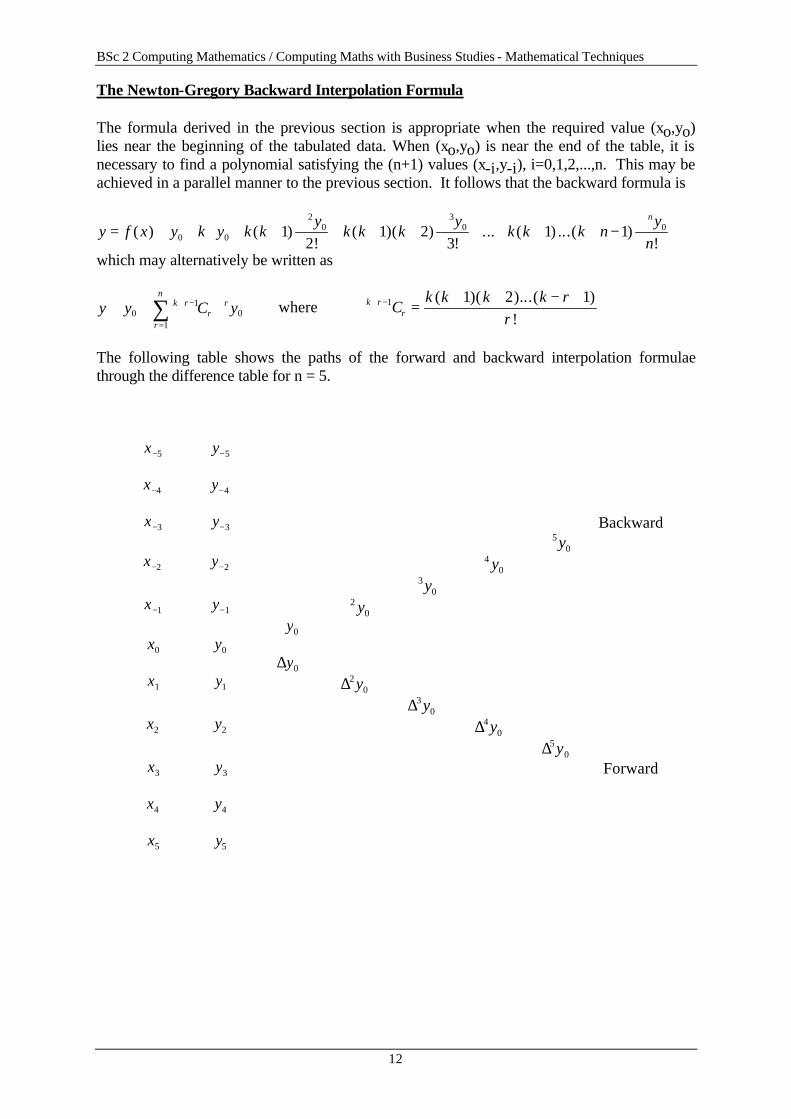
The following table shows the paths of the forward and backward interpolation formulae through the difference table for n = 5.

x−5 y−5

x−4 y−4

x−3 y−3 Backward ∇5

0y x−2 y−2 ∇4

0y ∇3

0y x−1 y−1 ∇2

0y ∇y0

x0 y0 ∆y0

x1 y1 ∆20y

∆30y

x2 y2 ∆40y

∆50y

x3 y3 Forward

x4 y4

x5 y5


13

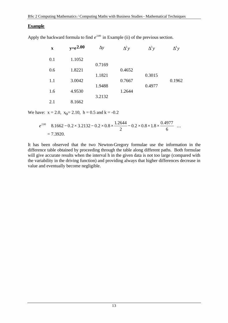
Example Apply the backward formula to find e2 00. in Example (ii) of the previous section.

x y=e2.00 ∆y ∆2 y ∆3 y ∆4 y

0.1 1.1052 0.7169

0.6 1.8221 0.4652 1.1821 0.3015

1.1 3.0042 0.7667 0.1962 1.9488 0.4977

1.6 4.9530 1.2644 3.2132

2.1 8.1662 We have: x = 2.0, xo= 2.10, h = 0.5 and k = -0.2

e2 00 8 1662 0 2 3 2132 0 2 0 81 2644

20 2 0 8 1 8

0 49776

. . . . . ..

. . ..

...≅ − × − × × − × × × +

= 7.3920. It has been observed that the two Newton-Gregory formulae use the information in the difference table obtained by proceeding through the table along different paths. Both formulae will give accurate results when the interval h in the given data is not too large (compared with the variability in the driving function) and providing always that higher differences decrease in value and eventually become negligible.


14

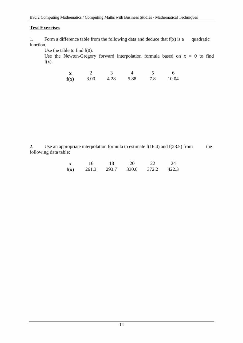
Test Exercises 1. Form a difference table from the following data and deduce that f(x) is a quadratic function. Use the table to find f(0). Use the Newton-Gregory forward interpolation formula based on x = 0 to find f(x).

x 2 3 4 5 6 f(x) 3.00 4.28 5.88 7.8 10.04

2. Use an appropriate interpolation formula to estimate f(16.4) and f(23.5) from the following data table:

x 16 18 20 22 24 f(x) 261.3 293.7 330.0 372.2 422.3


15

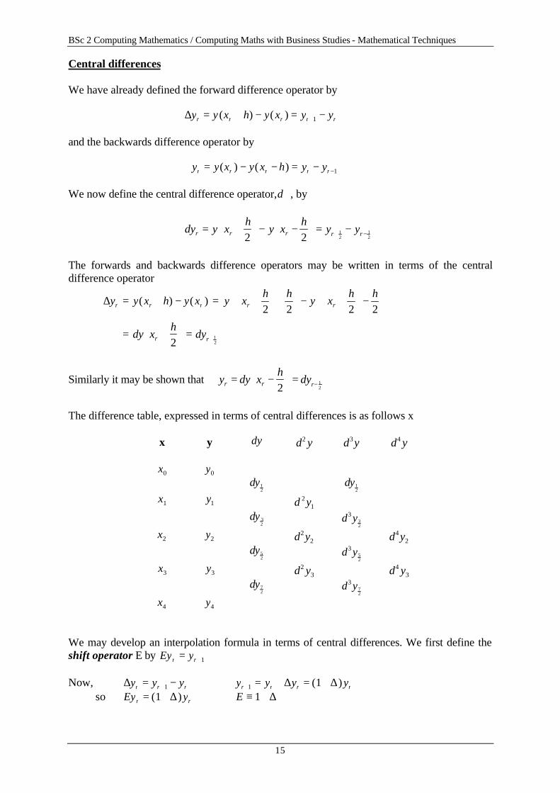
Central differences We have already defined the forward difference operator by ∆y y x h y x y yr r r r r= + − = −+( ) ( ) 1

and the backwards difference operator by ∇ = − − = − −y y x y x h y yr r r r r( ) ( ) 1

We now define the central difference operator,δ , by

δy y xh

y xh

y yr r r r r= +

− −

= −+ −2 212

12

The forwards and backwards difference operators may be written in terms of the central difference operator

∆yr = y x h y xr r( ) ( )+ − = y xh h

y xh h

r r+

+

− +

−

2 2 2 2

= δ δy xh

yr r+

= +212

Similarly it may be shown that ∇ = −

= −y y xh

yr r rδ δ2

12

The difference table, expressed in terms of central differences is as follows x

x y δy δ2 y δ3 y δ4 y

x0 y0 δy1

2 δy1

2

x1 y1 δ 21y

δy 32 δ3

32

y

x2 y2 δ22y δ4

2y δy5

2 δ3

52

y

x3 y3 δ23y δ4

3y δy7

2 δ3

72

y

x4 y4 We may develop an interpolation formula in terms of central differences. We first define the shift operator E by Ey yr r= +1 Now, ∆ ∆ ∆y y y y y y yr r r r r r r= − ∴ = + = ++ +1 1 1( ) so Ey y Er r= + ∴ ≡ +( )1 1∆ ∆


16

Also ∆y y E yr r r= =+δ δ12

12

Note that E y E y y E y E y y yr r r r r r r

12

12

12

12

12

12

1δ = − = − = −+ + +( )

so E y y E yr r

12

12δ δ= =∆ ⇒ the operators E and δ commute

∴ ∆ ≡ E

12δ

and E E≡ + ≡ +1 1

12∆ δ ∴ ∆2 2 21

212

121≡ ≡ ≡ +( )( ) ( )E E E Eδ δ δ δ δ

∴ ∆2 2 312≡ +δ δE

and ∆ ∆∆3 2 2 3 3 4 3 41

212

12

12

121≡ ≡ + ≡ + ≡ + +E E E E E Eδ δ δ δ δ δ δ δ( ) ( )

∴ ∆3 3 4 512

12≡ + +E Eδ δ δ

We may substitute in the Newton-Gregory forward formula y x khr( )+ = +( )1 ∆ k

ry

= + + − + − − +

1 1

21 2

3

2 3

k k k k k k yr∆∆ ∆

( )!

( )( )!

...

= + +−

+ +− −

+ + +

11

21 23

12

12

12

122 3 3 4 5kE

k kE

k k kE E yrδ δ δ δ δ δ

( )!

( )( )( )

!( ) ...

= + +−

+− −

+

11

21 23

12

122 3kE

k k k k kE yrδ δ δ

( )!

( )( )!

...

We now consider the relationship between backward differences and central differences. By definition ∇ = − ∴ = − ∇ = − ∇+ + + + +y y y y y y yr r r r r r r1 1 1 1 11( ) Also Ey yr r= +1 and y E yr r= −

+1

1 ∴ E − ≡ − ∇1 1( ) Also by definition ∇ = − = = ∴+ + +

−+y y y y E yr r r r r1 1 11

2

12δ δ ∇ ≡ −δE

12

or alternatively ∇ ≡ −δE

12

∇ = = = − ∇ = −− − − −2 1 2 2 21

212

121 1( )( ) ( ) ( )E E E Eδ δ δ δ δ δ

∴ ∇ = − −2 2 312δ δE

∇ ≡ − = − = − −− − − − − −3 2 3 3 1 4 3 41

212

12

12

121E E E E E Eδ δ δ δ δ δ δ δ( ) ( )

∴ ∇ ≡ − +− −3 3 4 512

12E Eδ δ δ

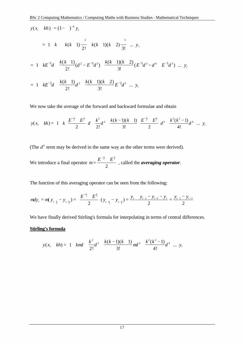
We may substitute in the Newton-Gregory backward formula


17

y x khr( )+ = − ∇ −( )1 kry

= + ∇ + +∇

+ + +∇

+

1 1

21 2

3

2 3

k k k k k k yr( )!

( )( )!

...

= + ++

− ++ +

− + +

− − − −11

21 23

12

12

12

122 3 3 4 5kE

k kE

k k kE E yrδ δ δ δ δ δ

( )!

( )( )( )

!( ) ...

= + ++

++ +

+

− −11

21 23

12

122 3kE

k k k k kE yrδ δ δ

( )!

( )( )!

...

We now take the average of the forward and backward formulae and obtain

y x kh kE E k k k k E E k k

yr r( )!

( )( )!

( )!

...+ = ++

+ +

− + +

+

−+

− −

12 2

1 13 2

14

12

12

12

122

2 32 2

4δ δ δ δ

(The δ4 term may be derived in the same way as the other terms were derived).

We introduce a final operator µ =+−E E

12

12

2 , called the averaging operator.

The function of this averaging operator can be seen from the following:

µδ µy y yE E

y yy y y y y y

r r r r rr r r r r r= − =

+

− =

+ − −=

−+ −

−

+ −+ − + −( ) ( )1

212

12

12

12

122 2 2

1 1 1 1

We have finally derived Stirling's formula for interpolating in terms of central differences. Stirling's formula

y x kh kk k k k k k

yr r( )!

( )( )!

( )!

...+ = + + +− +

+−

+

1

21 13

14

22 3

2 24µδ δ µδ δ


18

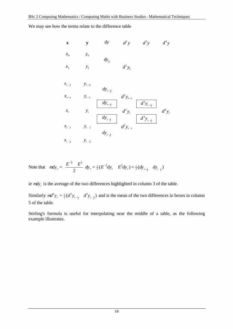
We may see how the terms relate to the difference table

x y δy δ2 y δ3 y δ4 y

x0 y0 δy1

2

x1 y1 δ21y

xr − 2 yr −2 δyr− 3

2

xr −1 yr −1 δ21yr−

δyr− 12 δ3

12

yr −

xr yr δ2 yr δ4 yr δyr+ 1

2 δ 3

12

yr+

xr +1 yr +1 δ21yr+

δyr+ 32

xr + 2 yr +2

Note that µδ δ δ δ δ δyE E

y E y E y y yr r r r r r=+

= + = +

−−

− +

12

12 1

212

12

122

12

12( ) ( )

ie µδyr is the average of the two differences highlighted in column 3 of the table. Similarly µδ δ δ3 1

23 3

12

12

y y yr r r= +− +( ) and is the mean of the two differences in boxes in column

5 of the table. Stirling's formula is useful for interpolating near the middle of a table, as the following example illustrates.


19

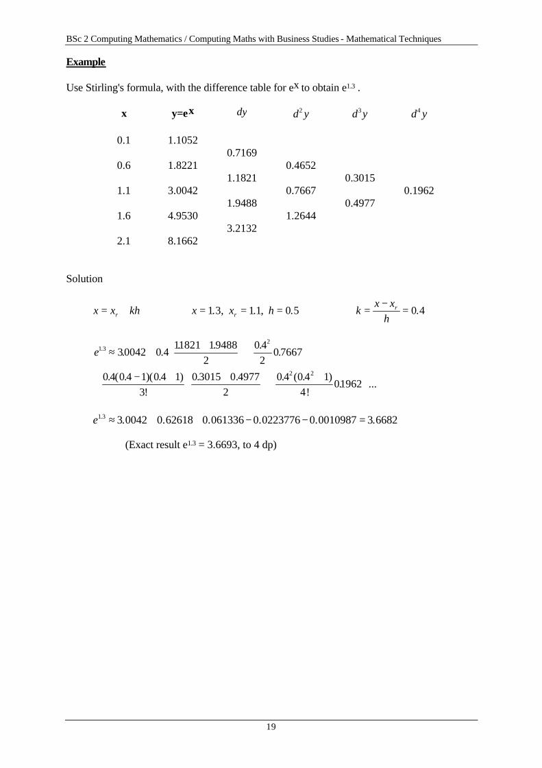
Example Use Stirling's formula, with the difference table for ex to obtain e1.3 .

x y=ex δy δ2 y δ3 y δ4 y

0.1 1.1052 0.7169

0.6 1.8221 0.4652 1.1821 0.3015

1.1 3.0042 0.7667 0.1962 1.9488 0.4977

1.6 4.9530 1.2644 3.2132

2.1 8.1662 Solution

x x kh x x h kx x

hr rr= + = = = =

−=1 3 1 1 0 5 0 4. , . , . .

e1 32

30042 0 411821 19488

20 4

20 7667. . .

. . ..≈ +

+

+

+− + +

++

+0 4 0 4 1 0 4 1

30 3015 0 4977

20 4 0 4 1

401962

2 2. ( . )( . )!

. . . ( . )!

. ...

∴ e1 3 3 0042 0 62618 0 061336 0 0223776 0 0010987 3 6682. . . . . . .≈ + + − − = (Exact result e1.3 = 3.6693, to 4 dp)


20

NUMERICAL DIFFERENTIATION Differentiation is a very important mathematical process and a great deal of effort has been devoted to the development of analytic techniques of finding the derivatives of various mathematical functions. It often occurs, however, that it is not possible to utilise these traditional methods. This happens when: (i) The function is too complex (ii) The function is unknown (when data are collected from some experiment). In this section numerical techniques are described which provide an estimate of the derivative of a tabulated function. Imagine that you have a procedure which computes a function f(x) and you want to find its derivative f'(x). Easy? The definition of the derivative is the limit, as h → 0 of

′ ≈+ −

f xf x h f x

h( )

( ) ( )

practically suggests an algorithm: Pick a small value h, evaluate f x f x h( ) ( ) and + and apply the above formula. The above procedure, however, contains two main sources of error: truncation error and roundoff error. The roundoff error depends upon the machine used to carry out the computation - it is necessary to ensure that the value used for h is exactly represented by the machine. Truncation error comes from the higher order terms in the Taylor series expansion:

f x h f x hf x h f x h f x( ) ( ) ( ) ( ) ( ) ...+ = + ′ + ′′ + ′′′ +12

2 16

3

which leads to f x h f x

hf x hf x

( ) ( )( ) ( ) ...

+ −= ′ + ′′ +1

2

We will investigate methods of using difference tables to evaluate the derivatives of a function numerically. From page 6, the Newton-Gregory forward polynomial is: f x P x f k f C f C fk n k

k kn

n( ) ( ) ....≈ = + + + +0 0 22

0 0∆ ∆ ∆ where k x x h= −( )0

Differentiating the above equation, remembering that dPdx

dPdk

dkdx

=

{ }′ ≈ ′ = + − + − + +f x P x f k f k k fk n k h( ) ( ) ( ) ( ) ...1

012

20

12

2 302 1 3 6 2∆ ∆ ∆

We can simplify this considerably if we take k = 0, giving a derivative corresponding to x x= 0

{ }′ ≈ − + − + − −f x f f f f fhn

nn( ) ... ( )0

10

12

20

13

30

14

40

101∆ ∆ ∆ ∆ ∆ (1)


21

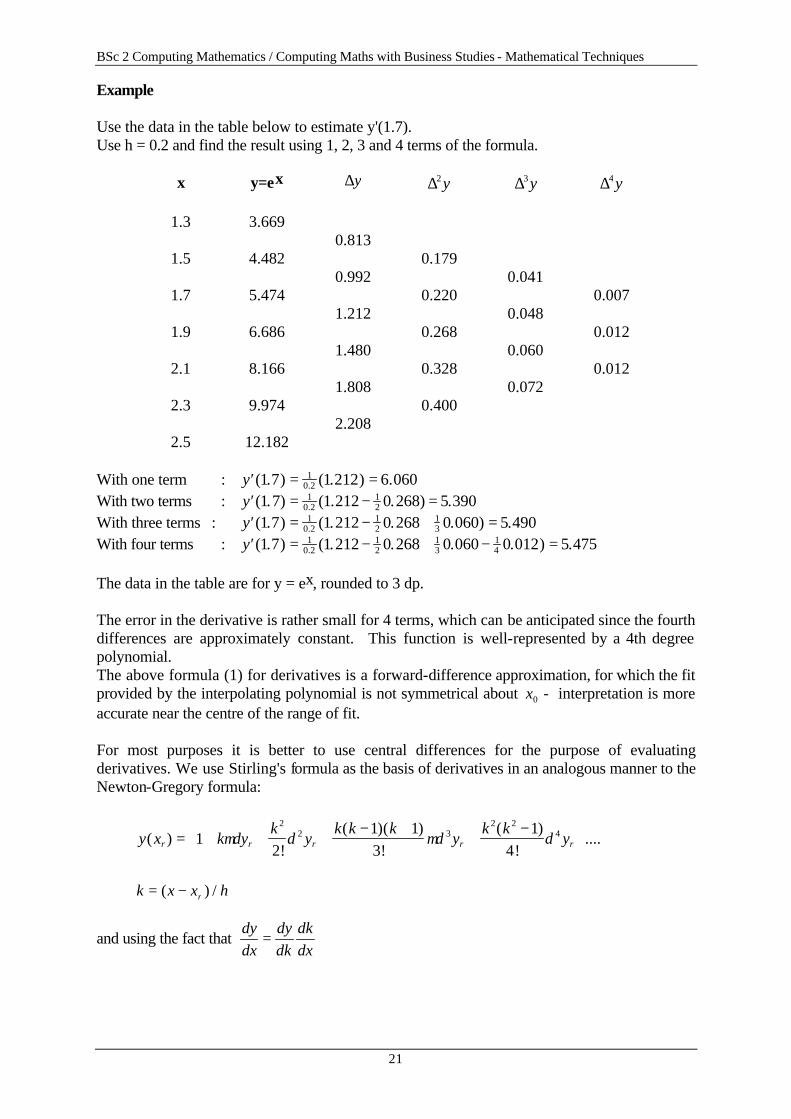
Example Use the data in the table below to estimate y'(1.7). Use h = 0.2 and find the result using 1, 2, 3 and 4 terms of the formula.

x y=ex ∆y ∆2 y ∆3 y ∆4 y

1.3 3.669 0.813

1.5 4.482 0.179 0.992 0.041

1.7 5.474 0.220 0.007 1.212 0.048

1.9 6.686 0.268 0.012 1.480 0.060

2.1 8.166 0.328 0.012 1.808 0.072

2.3 9.974 0.400 2.208

2.5 12.182 With one term : ′ = =y ( . ) ( . ) ..1 7 1 212 6 0601

0 2 With two terms : ′ = − =y ( . ) ( . . ) ..1 7 1 212 0 268 5 3901

0 212

With three terms : ′ = − + =y ( . ) ( . . . ) ..1 7 1 212 0 268 0 060 5 49010 2

12

13

With four terms : ′ = − + − =y ( . ) ( . . . . ) ..1 7 1 212 0 268 0 060 0 012 5 47510 2

12

13

14

The data in the table are for y = ex, rounded to 3 dp. The error in the derivative is rather small for 4 terms, which can be anticipated since the fourth differences are approximately constant. This function is well-represented by a 4th degree polynomial. The above formula (1) for derivatives is a forward-difference approximation, for which the fit provided by the interpolating polynomial is not symmetrical about x0 - interpretation is more accurate near the centre of the range of fit. For most purposes it is better to use central differences for the purpose of evaluating derivatives. We use Stirling's formula as the basis of derivatives in an analogous manner to the Newton-Gregory formula:

y x k yk

yk k k

yk k

yr r r r r( )!

( )( )!

( )!

....= + + +− +

+−

+

12

1 13

14

22 3

2 24µδ δ µδ δ

k x x hr= −( ) /

and using the fact that dydx

dydk

dkdx

=


22

Differentiating gives ′ = + +−

+−

+

y xh

k yk

yk k

yr r r r( )! !

...1 3 1

34 2

42

23

34µδ δ µδ µδ

Using d ydx

ddx

dydx

ddk

dydx

dkdx

ddk

dydx h

2

2

1= = = we obtain

′′ = + +−

+

y xh

yk

yk

yr r r r( )! !

...1 6

312 2

422 3

24δ µδ δ

= + +−

1 12 242

2 32

4

hy k y

kyr r rδ µδ δ

!

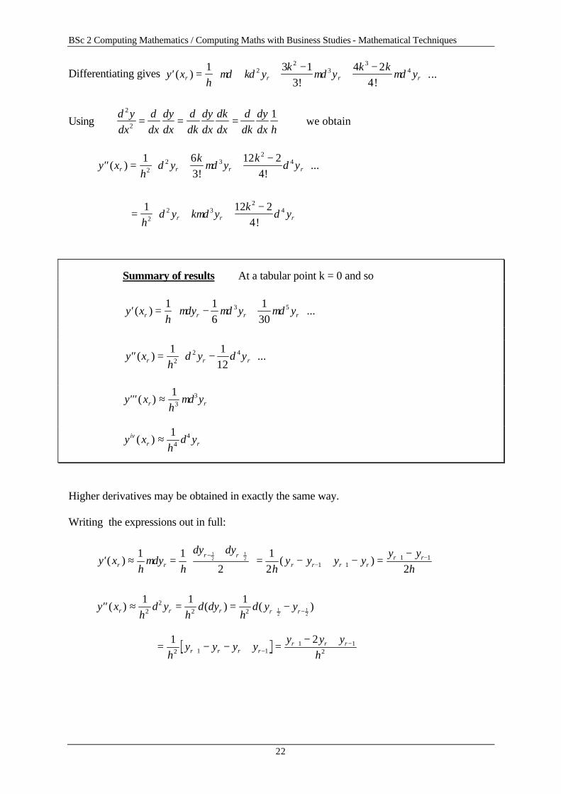
Summary of results At a tabular point k = 0 and so

′ = − + +

y xh

y y yr r r r( ) ...1 1

6130

3 5µδ µδ µδ

′′ = − +

y xh

y yr r r( ) ...1 1

1222 4δ δ

′′′ ≈y xh

yr r( )1

33µδ

y xh

yivr r( ) ≈

14

4δ

Higher derivatives may be obtained in exactly the same way. Writing the expressions out in full:

′ ≈ =+

= − + − =−− +

− ++ −y x

hy

h

y y

hy y y y

y yhr r

r rr r r r

r r( ) ( )1 1

21

2 2

12

12

1 11 1µδ

δ δ

′′ ≈ = = −+ −y xh

yh

yh

y yr r r r r( ) ( ) ( )1 1 1

22

2 2 12

12

δ δ δ δ

= − − + =− +

+ −+ −1 2

2 1 11 1

2hy y y y

y y yhr r r r

r r r


23

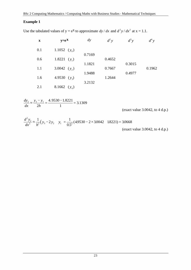
Example 1 Use the tabulated values of y = ex to approximate dy dx/ and d y dx2 2/ at x = 1.1.

x y=ex δy δ2 y δ3 y δ4 y

0.1 1.1052 ( y0 ) 0.7169

0.6 1.8221 ( y1) 0.4652 1.1821 0.3015

1.1 3.0042 ( y2 ) 0.7667 0.1962 1.9488 0.4977

1.6 4.9530 ( y3) 1.2644 3.2132

2.1 8.1662 ( y4 ) dydx

y yh

2 3 1

24 9530 1 8221

13 1309≈

−=

−=

. ..

(exact value 3.0042, to 4 d.p.)

( )d ydx h

y y y2

22 2 3 2 1 2

12

10 5

49530 2 30042 18221 30668≈ − + = − × + =.

( . . . ) .

(exact value 3.0042, to 4 d.p.)


24

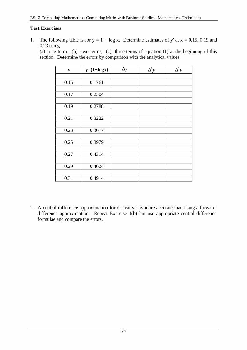
Test Exercises 1. The following table is for y = 1 + log x. Determine estimates of y' at x = 0.15, 0.19 and

0.23 using (a) one term, (b) two terms, (c) three terms of equation (1) at the beginning of this

section. Determine the errors by comparison with the analytical values.

x y=(1+logx) ∆y ∆2 y ∆3 y

0.15 0.1761

0.17 0.2304

0.19 0.2788

0.21 0.3222

0.23 0.3617

0.25 0.3979

0.27 0.4314

0.29 0.4624

0.31 0.4914 2. A central-difference approximation for derivatives is more accurate than using a forward-

difference approximation. Repeat Exercise 1(b) but use appropriate central difference formulae and compare the errors.


25

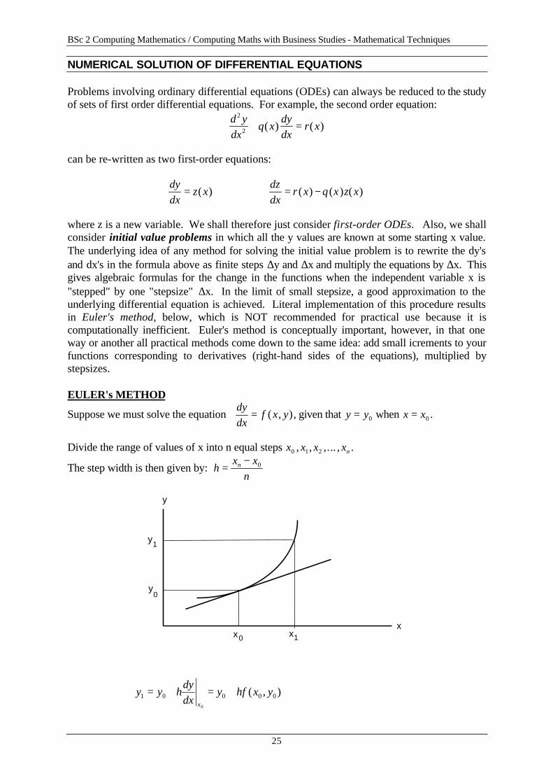
NUMERICAL SOLUTION OF DIFFERENTIAL EQUATIONS Problems involving ordinary differential equations (ODEs) can always be reduced to the study of sets of first order differential equations. For example, the second order equation:

d ydx

q xdydx

r x2

2 + =( ) ( )

can be re-written as two first-order equations:

dydx

z x= ( ) dzdx

r x q x z x= −( ) ( ) ( )

where z is a new variable. We shall therefore just consider first-order ODEs. Also, we shall consider initial value problems in which all the y values are known at some starting x value. The underlying idea of any method for solving the initial value problem is to rewrite the dy's and dx's in the formula above as finite steps ∆y and ∆x and multiply the equations by ∆x. This gives algebraic formulas for the change in the functions when the independent variable x is "stepped" by one "stepsize" ∆x. In the limit of small stepsize, a good approximation to the underlying differential equation is achieved. Literal implementation of this procedure results in Euler's method, below, which is NOT recommended for practical use because it is computationally inefficient. Euler's method is conceptually important, however, in that one way or another all practical methods come down to the same idea: add small icrements to your functions corresponding to derivatives (right-hand sides of the equations), multiplied by stepsizes. EULER's METHOD

Suppose we must solve the equation dydx

f x y= ( , ), given that y y= 0 when x x= 0 .

Divide the range of values of x into n equal steps x x x xn0 1 2, , ,... , .

The step width is then given by: hx x

nn=

− 0

y

y

x xx

y

0

0

1

1

y y hdydx

y hf x yx

1 0 0 0 0

0

= + = + ( , )


26

y y hf x y2 1 1 1= + ( , ) M M M y y hf x yn n n n= +− − −1 1 1( , )

Example 1 dydx

y x= −2 Find y(2.3) given y(2)=3.

Take h=0.1 : y y y x1 0 0

200 1= + −. ( ) x y0 02 3= =,

( )y y y xi i i i+ = + −1201.

i xi yi yi2 yi

2-xi 0.1(yi2-xi

) yi+1 0 2.0 3.000 1 2.1 2 2.2 3 2.3

i xi yi yi2 yi

2-xi 0.1(yi2-xi

) yi+1 0 2.0 3.000 9.000 7.000 0.700 3.700 1 2.1 3.700 13.690 11.590 1.159 4.859 2 2.2 4.859 23.610 21.410 2.141 7.000 3 2.3 7.000


27

Example 2 dydx

x y= + Find y(0.05) correct to 5 d.p. given that y(0)=2

Take h=0.01: ( )y y x yi i+ = + +1 0 00 01. , y x0 02 0= =, ∴ y y yi i i+ = +1 0 01. '

i xi yi yi' 0.01yi' yi+1 0 0.00 2 2 0.02 2.02 1 0.01 2.02 2.03 0.0203 2.0403 2 0.02 2.0403 2.0603 0.020603 2.060903 3 0.03 2.060903 2.090903 0.02090903 2.08181203 4 0.04 2.08181203 2.12181203 0.0212181203 2.1030301503 5 0.05 2.1030301503

Example 3 dydx

x y= + −2 1( ) Find y for x=2.0(0.2)3.0, given y(2)=5

Take h=0.2 y y yi i i+ = +1 0 2. '

i xi yi yi' 0 2 5 1 1 2.2 5.2 1.2 2 2.4 5.44 1.36 3 2.6 5.712 1.488 4 2.8 6.0096 1.5904 5 3.0 6.32768


28

Example 4 dydx

x y= + −1 Find y for x=1.0(0.2)2.0, given y(1)=2

Take h=0.2 y y yi i i+ = +1 0 2. '

i xi yi yi' 0 1.0 2 0 1 1.2 2 0.2 2 1.4 2.04 0.36 3 1.6 2.112 0.488 4 1.8 2.2096 0.5904 5 2.0 2.32768 0.67232

EXERCISES Solve the following ODEs to obtain the required values of y, under the given initial conditions:

1. If dydx

x y= + find y for x=0,(0.1),0.5, given that y(0)=1.

(Solution: 1.0, 1.1, 1.22, 1.362, 1.5282, 1.72102)

2. If dydx

xy= +1 find y for x=0,(0.1),0.5, given that y(0)=1.

(Solution: 1.0, 1.1, 1.211, 1.3352, 1.4753, 1.6343) 3. Solve the above two equations by analytic methods and check your numerical results from

questions 1 and 2.


29

SECOND-ORDER ODEs To solve first order ODEs, one boundary/initial condition was required; for second order ODEs it becomes necessary to have two. We approximate the second derivative by the first term of the central difference formula presented earlier in this booklet. We can see from the following diagram how this can be derived geometrically:

A

B

C

y y y

x x x

-1 0 1

-1 0 1 Approximate slope at B may be given by:

(1) BC: dydx

y yh

≈−1 0 (Forward difference)

(2) AB: dydx

y yh

≈− −0 1 (Backward difference)

(3) AC: dydx

y yh

≈− −1 1

2 (Central difference)

For the second derivative: d ydx

y yh

y yh

hy y y

h

2

2

1 0 0 1

1 0 12

2≈

− − −

=− +

−

−


30

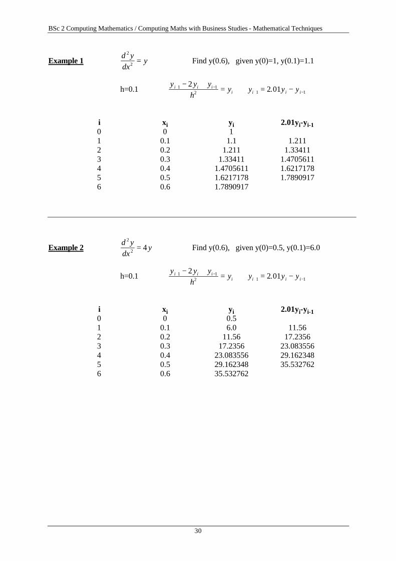
Example 1 d ydx

y2

2 = Find y(0.6), given y(0)=1, y(0.1)=1.1

h=0.1 y y y

hyi i i

i+ −− +

=1 12

2 ⇒ y y yi i i+ −= −1 12 01.

i xi yi 2.01yi-yi-1 0 0 1 1 0.1 1.1 1.211 2 0.2 1.211 1.33411 3 0.3 1.33411 1.4705611 4 0.4 1.4705611 1.6217178 5 0.5 1.6217178 1.7890917 6 0.6 1.7890917

Example 2 d ydx

y2

2 4= Find y(0.6), given y(0)=0.5, y(0.1)=6.0

h=0.1 y y y

hyi i i

i+ −− +

=1 12

2 ⇒ y y yi i i+ −= −1 12 01.

i xi yi 2.01yi-yi-1 0 0 0.5 1 0.1 6.0 11.56 2 0.2 11.56 17.2356 3 0.3 17.2356 23.083556 4 0.4 23.083556 29.162348 5 0.5 29.162348 35.532762 6 0.6 35.532762


31

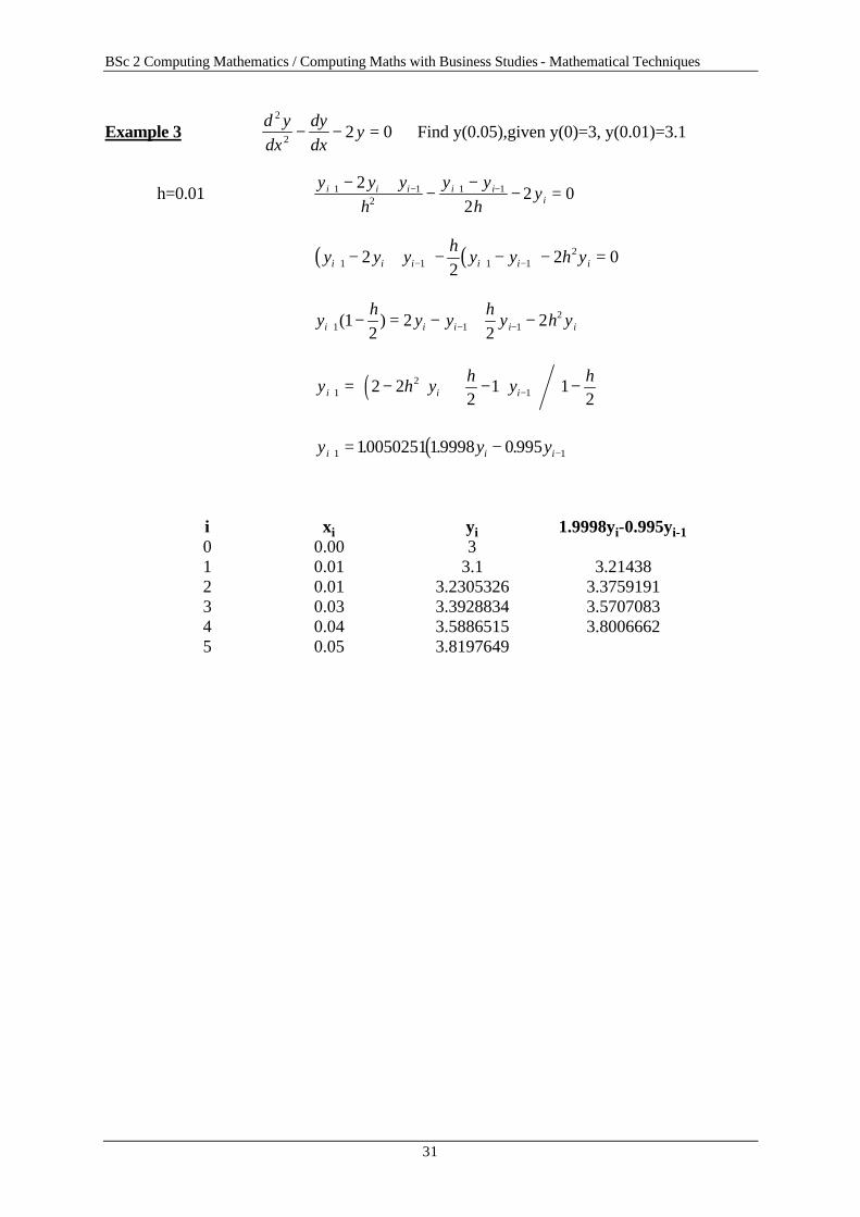
Example 3 d ydx

dydx

y2

2 2 0− − = Find y(0.05),given y(0)=3, y(0.01)=3.1

h=0.01 ∴ y y y

hy y

hyi i i i i

i+ − + −− +

−−

− =1 12

1 122

2 0

∴ ( ) ( )y y yh

y y h yi i i i i i+ − + −− + − − − =1 1 1 122

22 0

∴ yh

y yh

y h yi i i i i+ − −− = − + −1 1 121

22

22( )

∴ ( )y h y h y hi i i+ −= − + −

−

1

212 2

21 1

2

∴ ( )y y yi i i+ −= −1 110050251 19998 0 995. . .

i xi yi 1.9998yi-0.995yi-1 0 0.00 3 1 0.01 3.1 3.21438 2 0.01 3.2305326 3.3759191 3 0.03 3.3928834 3.5707083 4 0.04 3.5886515 3.8006662 5 0.05 3.8197649


32

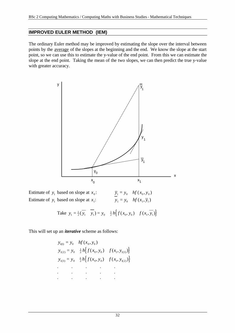
IMPROVED EULER METHOD (IEM) The ordinary Euler method may be improved by estimating the slope over the interval between points by the average of the slopes at the beginning and the end. We know the slope at the start point, so we can use this to estimate the y-value of the end point. From this we can estimate the slope at the end point. Taking the mean of the two slopes, we can then predict the true y-value with greater accuracy.

y

y

y

x x

y

0 1

0

1

_

1

1

__

x

y

Estimate of y1 based on slope at x0 : y y hf x y1 0 0 0= + ( , )

Estimate of y1 based on slope at x1: y y hf x y1 0 1 1= + ( , ) Take { }y y y y h f x y f x y1

12 1 1 0

12 0 0 1 1= + = + +( ) ( , ) ( , )

This will set up an iterative scheme as follows: y y hf x y1 1 0 0 0( ) ( , )= +

{ }y y h f x y f x y1 2 012 0 0 1 1 1( ) ( )( , ) ( , )= + +

{ }y y h f x y f x y1 3 012 0 0 1 1 2( ) ( )( , ) ( , )= + +

. . . . . . . . . . . . . . .


33

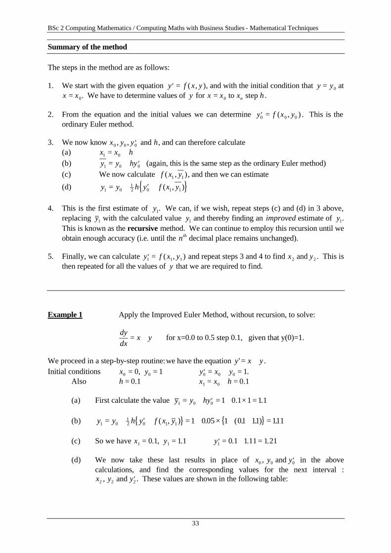
Summary of the method The steps in the method are as follows: 1. We start with the given equation ′ =y f x y( , ), and with the initial condition that y y= 0 at

x x= 0. We have to determine values of y for x x x hn= 0 to step . 2. From the equation and the initial values we can determine ′ =y f x y0 0 0( , ) . This is the

ordinary Euler method. 3. We now know x y y h0 0 0, , ′ and , and can therefore calculate (a) x x h1 0= + (b) y y hy1 0 0= + ′ (again, this is the same step as the ordinary Euler method) (c) We now calculate f x y( , )1 1 , and then we can estimate

(d) { }y y h y f x y1 012 0 1 1= + ′ + ( , )

4. This is the first estimate of y1. We can, if we wish, repeat steps (c) and (d) in 3 above,

replacing y1 with the calculated value y1 and thereby finding an improved estimate of y1. This is known as the recursive method. We can continue to employ this recursion until we obtain enough accuracy (i.e. until the nth decimal place remains unchanged).

5. Finally, we can calculate ′ =y f x y1 1 1( , ) and repeat steps 3 and 4 to find x y2 2 and . This is

then repeated for all the values of y that we are required to find. Example 1 Apply the Improved Euler Method, without recursion, to solve:

dydx

x y= + for x=0.0 to 0.5 step 0.1, given that y(0)=1.

We proceed in a step-by-step routine: we have the equation y x y'= + . Initial conditions ⇒ x y0 00 1= =, ∴ ′ = + =y x y0 0 0 1. Also h = 0 1. ∴ = + =x x h1 0 0 1. (a) First calculate the value y y hy1 0 0 1 0 1 1 1 1= + ′ = + × =. . (b) { } { }y y h y f x y1 0

12 0 1 1 1 0 05 1 01 11 111= + ′ + = + × + + =( , ) . ( . . ) .

(c) So we have x y y1 1 10 1 1 1 0 1 1 11 1 21= = ∴ ′ = + =. , . . . .

(d) We now take these last results in place of x y y0 0 0, and ′ in the above calculations, and find the corresponding values for the next interval : x y y2 2 2, and ′ . These values are shown in the following table:


34

n xn yn ′yn 0 0.0 1.0 1.0 1 0.1 1.11 1.21 2 0.2 1.24205 1.44205 3 0.3 1.398465 1.698465 4 0.4 1.581804 1.981804 5 0.5 1.794893 2.294893

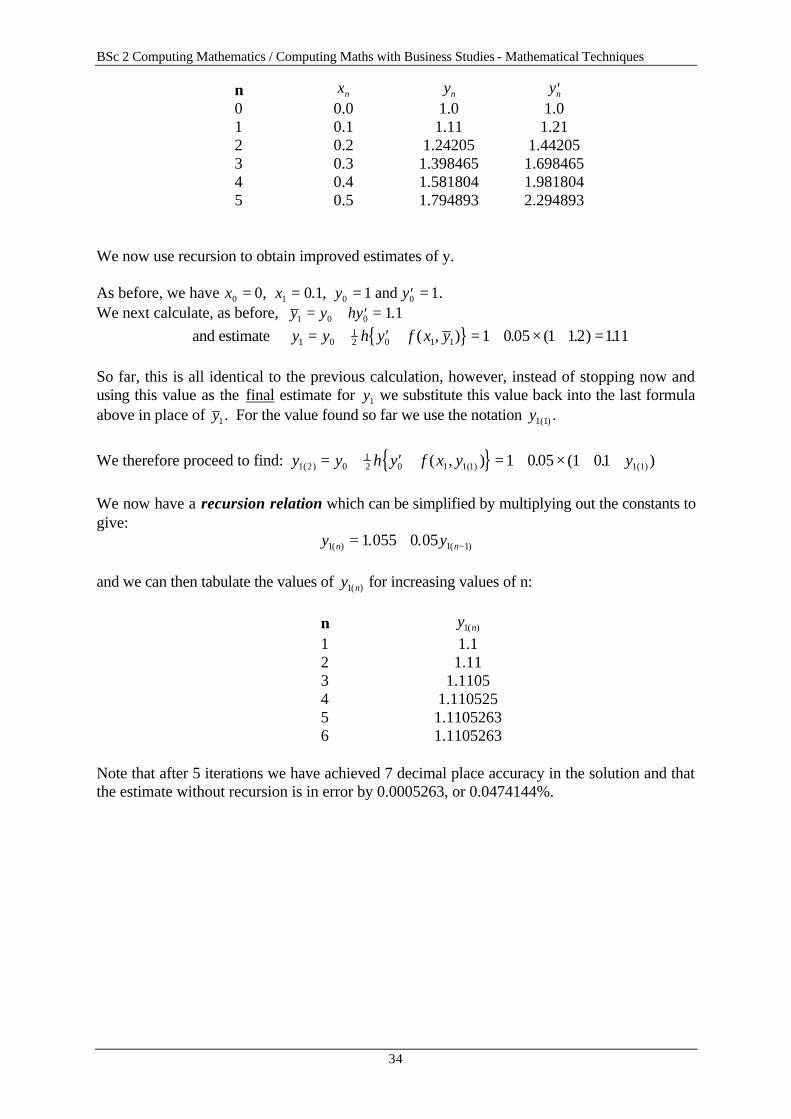
We now use recursion to obtain improved estimates of y. As before, we have x x y y0 1 0 00 0 1 1 1= = = ′ =, . , and . We next calculate, as before, y y hy1 0 0 1 1= + ′ = . and estimate { }y y h y f x y1 0

12 0 1 1 1 0 05 1 12 111= + ′ + = + × + =( , ) . ( . ) .

So far, this is all identical to the previous calculation, however, instead of stopping now and using this value as the final estimate for y1 we substitute this value back into the last formula above in place of y1. For the value found so far we use the notation y1 1( ) . We therefore proceed to find: { }y y h y f x y y1 2 0

12 0 1 1 1 1 11 0 05 1 01( ) ( ) ( )( , ) . ( . )= + ′ + = + × + +

We now have a recursion relation which can be simplified by multiplying out the constants to give:

y yn n1 1 11 055 0 05( ) ( ). .= + − and we can then tabulate the values of y n1( ) for increasing values of n:

n y n1( ) 1 1.1 2 1.11 3 1.1105 4 1.110525 5 1.1105263 6 1.1105263

Note that after 5 iterations we have achieved 7 decimal place accuracy in the solution and that the estimate without recursion is in error by 0.0005263, or 0.0474144%.


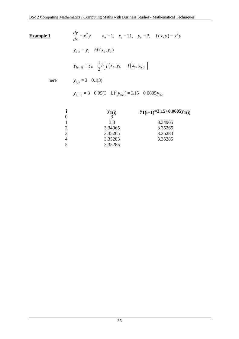
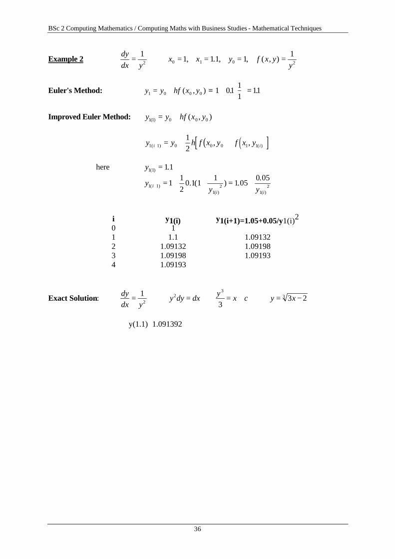
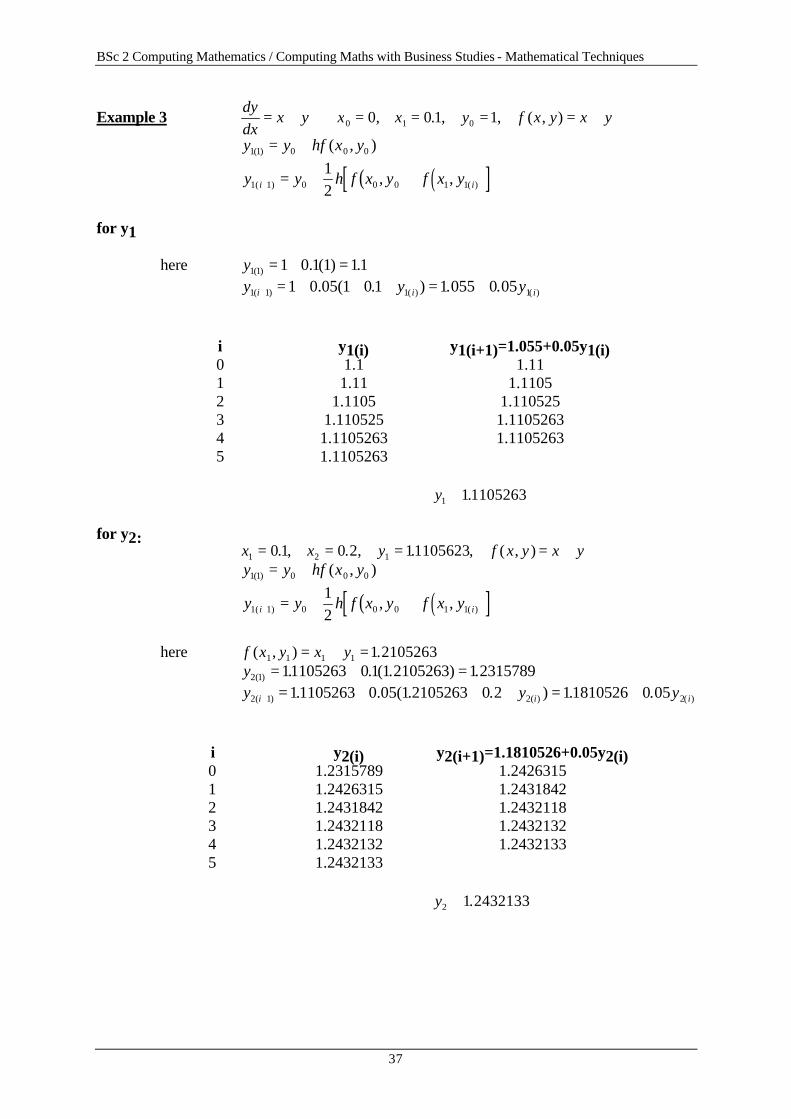
35

Example 1 dydx

x y= 2 x x y f x y x y0 1 021 11 3= = = =, . , , ( , )

y y hf x y1 1 0 0 0( ) ( , )= +

( ) ( )[ ]y y h f x y f x yi i1 1 0 0 0 1 1

12( ) ( ), ,+ = + +

here y1 1 3 0 1 3( ) . ( )= + y y yi i i1 1

21 13 0 05 3 11 315 0 0605( ) ( ) ( ). ( . ) . .+ = + + = +

i y1(i) y1(i+1)=3.15+0.0605y1(i) 0 3 1 3.3 3.34965 2 3.34965 3.35265 3 3.35265 3.35283 4 3.35283 3.35285 5 3.35285


36

Example 2 dydx y

=1

2 x x y f x yy0 1 0 21 1 1 11

= = = =, . , , ( , )

Euler's Method: y y hf x y1 0 0 0= + ( , ) = 1 0111

11+

=. .

Improved Euler Method: y y hf x y1 1 0 0 0( ) ( , )= +

( ) ( )[ ]y y h f x y f x yi i1 1 0 0 0 1 1

12( ) ( ), ,+ = + +

here y1 1 1 1( ) .=

yy yi

i i1 1

12

121

12

0 1 11

1 050 05

( )( ) ( )

. ( ) ..

+ = + + = +

i y1(i) y1(i+1)=1.05+0.05/y1(i)2 0 1 1 1.1 1.09132 2 1.09132 1.09198 3 1.09198 1.09193 4 1.09193

Exact Solution: dydx y

y dy dx y x c y x= ∴ = = + ∴ = −13

3 222

33

∴ y(1.1)≅1.091392


37

Example 3 dydx

x y= + x x y f x y x y0 1 00 0 1 1= = = = +, . , , ( , )

y y hf x y1 1 0 0 0( ) ( , )= +

( ) ( )[ ]y y h f x y f x yi i1 1 0 0 0 1 1

12( ) ( ), ,+ = + +

for y1 here y1 1 1 0 1 1 11( ) . ( ) .= + = y y yi i i1 1 1 11 0 05 1 0 1 1 055 0 05( ) ( ) ( ). ( . ) . .+ = + + + = +

i y1(i) y1(i+1)=1.055+0.05y1(i) 0 1.1 1.11 1 1.11 1.1105 2 1.1105 1.110525 3 1.110525 1.1105263 4 1.1105263 1.1105263 5 1.1105263

∴ y1 11105263≅ . for y2: x x y f x y x y1 2 10 1 0 2 11105623= = = = +. , . , . , ( , ) y y hf x y1 1 0 0 0( ) ( , )= +

( ) ( )[ ]y y h f x y f x yi i1 1 0 0 0 1 1

12( ) ( ), ,+ = + +

here f x y x y( , ) .1 1 1 1 1 2105263= + = y2 1 11105263 0 1 1 2105263 1 2315789( ) . . ( . ) .= + = y y yi i i2 1 2 211105263 0 05 1 2105263 0 2 11810526 0 05( ) ( ) ( ). . ( . . ) . .+ = + + + = +

i y2(i) y2(i+1)=1.1810526+0.05y2(i) 0 1.2315789 1.2426315 1 1.2426315 1.2431842 2 1.2431842 1.2432118 3 1.2432118 1.2432132 4 1.2432132 1.2432133 5 1.2432133

∴ y2 1 2432133≅ .


38

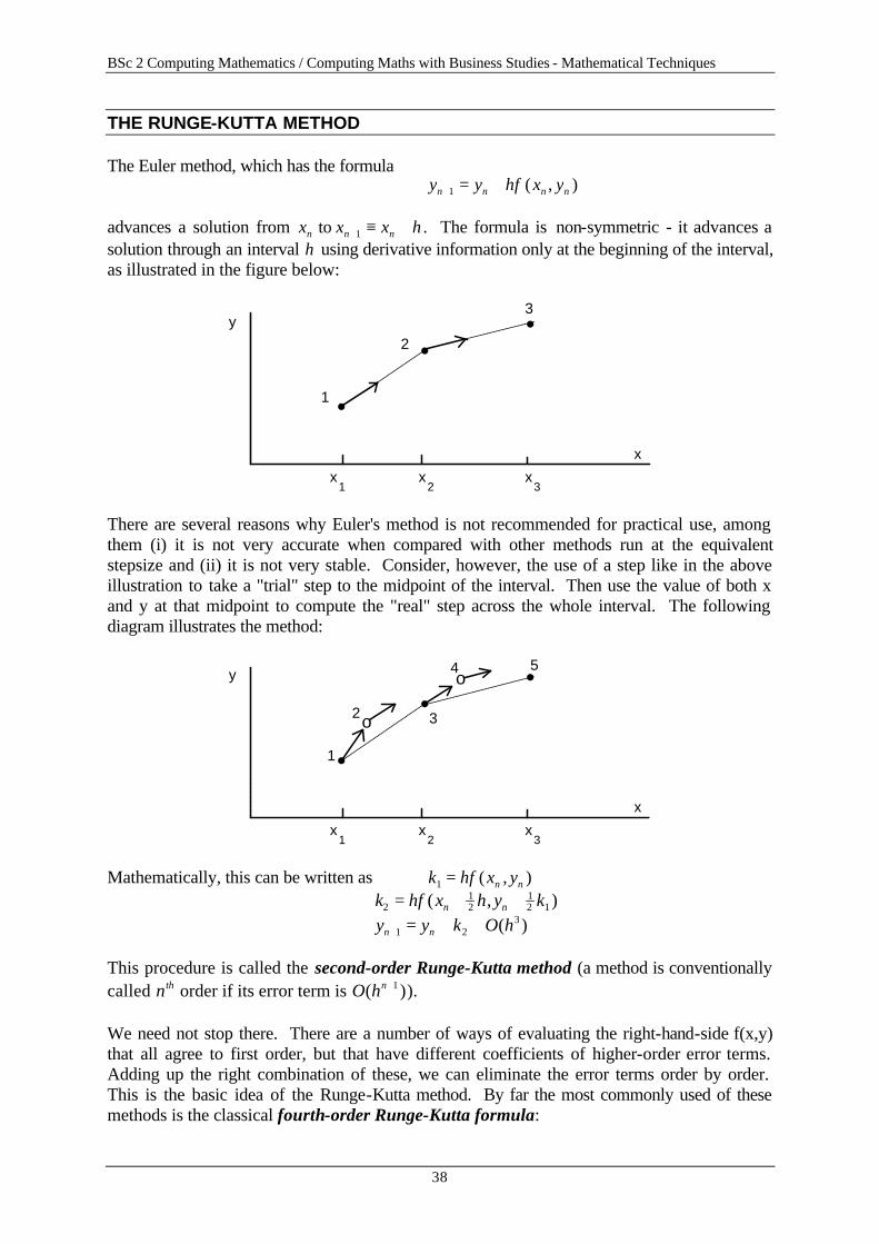
THE RUNGE-KUTTA METHOD The Euler method, which has the formula y y hf x yn n n n+ = +1 ( , ) advances a solution from x x x hn n n to + ≡ +1 . The formula is non-symmetric - it advances a solution through an interval h using derivative information only at the beginning of the interval, as illustrated in the figure below:

l

l

l1

2

3

x x x1 2 3

x

y

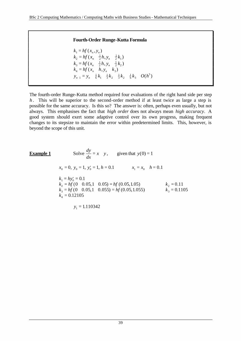
There are several reasons why Euler's method is not recommended for practical use, among them (i) it is not very accurate when compared with other methods run at the equivalent stepsize and (ii) it is not very stable. Consider, however, the use of a step like in the above illustration to take a "trial" step to the midpoint of the interval. Then use the value of both x and y at that midpoint to compute the "real" step across the whole interval. The following diagram illustrates the method:

l

l

l1

3

5

x x x1 2 3

x

y

o

o

2

4

Mathematically, this can be written as k hf x yn n1 = ( , ) k hf x h y kn n2

12

12 1= + +( , )

y y k O hn n+ = + +1 23( )

This procedure is called the second-order Runge-Kutta method (a method is conventionally called nth order if its error term is O hn( )+1 ). We need not stop there. There are a number of ways of evaluating the right-hand-side f(x,y) that all agree to first order, but that have different coefficients of higher-order error terms. Adding up the right combination of these, we can eliminate the error terms order by order. This is the basic idea of the Runge-Kutta method. By far the most commonly used of these methods is the classical fourth-order Runge-Kutta formula:


39

Fourth-Order Runge-Kutta Formula k hf x yn n1 = ( , ) k hf x h y kn n2

12

12 1= + +( , )

k hf x h y kn n312

12 2= + +( , )

k hf x h y kn n4 3= + +( , ) y y k k k k O hn n+ = + + + + +1

16 1

13 2

13 2

16 3

5( ) The fourth-order Runge-Kutta method required four evaluations of the right hand side per step h . This will be superior to the second-order method if at least twice as large a step is possible for the same accuracy. Is this so? The answer is: often, perhaps even usually, but not always. This emphasises the fact that high order does not always mean high accuracy. A good system should exert some adaptive control over its own progress, making frequent changes to its stepsize to maintain the error within predetermined limits. This, however, is beyond the scope of this unit.

Example 1 Solve dydx

x y= + , given that y( )0 1=

x y y h x x h0 0 0 1 00 1 1 0 1 0 1= = ′ = = = + =, , , . . k hy1 0 0 1= ′ = . k hf hf k2 20 0 05 1 0 05 0 05 1 05 0 11= + + = ∴ =( . , . ) ( . , . ) . k hf hf k3 30 0 05 1 0 055 0 05 1 055 0 1105= + + = ∴ =( . , . ) ( . , . ) . k4 0 12105= . ∴ =y1 1 110342.


40

Exercises 1. Using the 4th order Runge Kutta method, (a) compute an estimate of x(0.75) for the initial value problem:

dxdt

x t xt x= + + =, ( )0 1

using a step size of h = 0 15. . (Solution: 3.2345)

(b) compute an estimate of x(2) for the initial value problem

dxdt x t

=+1

, x( )1 2=

using a step size of h = 0 1. . (Solution: 2.2771)

2. Solve ′ = +y x y with y x= =1 0 at . Determine the function values for y for x=0(0.1)0.5.

(Solution: 1.0,1.110342,1.242806,1.399718,1.583649,1.797442) 3. Solve ′ = −y y xy2 with y x= =0 4 0. . at Determine the function values for y for x=0(0.2)1.0.

(Solution: 0.4, 0.4259, 0.4374, 0.4319, 0.4085, 0.3689)

4. Solve ′ =−+

yy xy x

with y x= =1 0 at .

Determine the function values for y for x=0(0.2)1.0. (Solution: 1.0, 1.1679, 1.2902, 1.3817, 1.4497, 1.4983)

Date post:	15-Apr-2018
Category:	Documents
Upload:	dangthien
View:	251 times
Download:	0 times

NUMERICAL METHODS CONTENTS - Orange -...

Documents