53
Numerical Methods for Differential Equations Chapter 5: Elliptic and Parabolic PDEs Gustaf S¨ oderlind Numerical Analysis, Lund University
| Date post: | 25-Jun-2018 |
| Category: |
Documents |
| Upload: | phamkhuong |
| View: | 214 times |
| Download: | 0 times |

Numerical Methods for Differential EquationsChapter 5: Elliptic and Parabolic PDEs
Gustaf SoderlindNumerical Analysis, Lund University

Contents V4.16
1. Brief overview of PDE problems
2. Elliptic problems with FDM
3. Elliptic problems with cG(1) FEM
4. Parabolic problems
5. Method of lines
6. Error analysis and convergence
7. Parabolic problems with cG(1) FEM
8. Well-posedness
2 / 53

1. Brief overview of PDE problems
Classification Three basic types, four prototype equations
Elliptic −∆u = f + BC Poisson equation
Parabolic ut = ∆u + BC & IV Diffusion equation
Hyperbolic utt = ∆u + BC & IV Wave equationut + a(u)ux = 0 + BC & IV Advection equation
We will consider these equations in 1D (one space dimension only)
−u′′ = f ; ut = uxx ; utt = uxx ; ut + a(u)ux = 0
3 / 53

Classification of PDEs
Classical approach Linear PDE with two independent variables
Auxx + 2Buxy + Cuyy + L(ux , uy , u, x , y) = 0
with L linear in ux , uy , u. Study
δ := det
(A BB C
)= AC − B2
δ > 0 Ellipticδ = 0 Parabolicδ < 0 Hyperbolic
4 / 53

General classification of PDEs Fourier transforms
Highest derivatives wrt t and x determines the PDE type
Let F (ω, x) = eiωx and let u and its derivatives go to zero asx → ±∞, and introduce the Fourier transform F : u 7→ u by
u(ω) = Fu = 〈F , u〉 =
∫ ∞−∞
F u dx =
∫ ∞−∞
e−iωxu dx
Then
Fut = 〈F , ut〉 = d(Fu)/dt = du/dt
Fux = 〈F , ux〉 = −〈Fx , u〉 = −〈iωF , u〉 = iωFu = iω u
Fuxx = 〈F , uxx〉 = 〈Fxx , u〉 = −〈ω2F , u〉 = −ω2Fu = (iω)2 u
etc.
5 / 53

General classification. . .
Highest order terms (real coefficients)
∂pu
∂tp=∂qu
∂xq
Hyperbolic if p + q is even, parabolic if p + q is odd
ut = ux Hyperbolicut = uxx Paraboliciut = uxx Hyperbolicut = uxxx Hyperbolicut = −uxxxx Parabolic
utt = uxx Hyperbolicutt = −uxxxx Hyperbolic
6 / 53
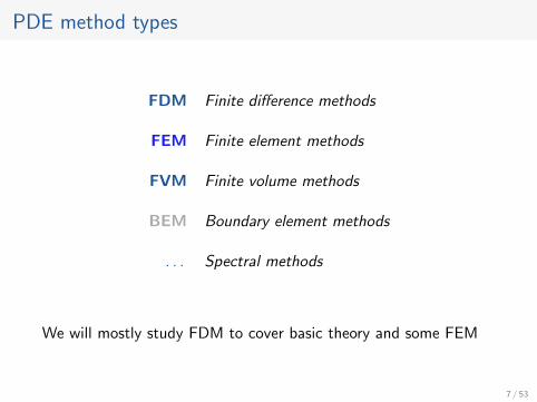
PDE method types
FDM Finite difference methods
FEM Finite element methods
FVM Finite volume methods
BEM Boundary element methods
. . . Spectral methods
We will mostly study FDM to cover basic theory and some FEM
7 / 53

PDE methods for elliptic problems
Simple geometry FDM or Fourier methodsComplex geometry FEMSpecial problems FVM or BEM
Very large, sparse systems, e.g. 106 — 1010 equations
Often combined with iterative solvers such as multigrid methods
8 / 53
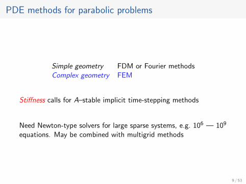
PDE methods for parabolic problems
Simple geometry FDM or Fourier methodsComplex geometry FEM
Stiffness calls for A–stable implicit time-stepping methods
Need Newton-type solvers for large sparse systems, e.g. 106 — 109
equations. May be combined with multigrid methods
9 / 53

PDE methods for hyperbolic problems
FDM, FVM. Sometimes FEM
Very challenging problems, with conservation properties, sometimesshocks, and sometimes multiscale phenomena such as turbulence
Solutions may be discontinuous, cf. “sonic booms”
Highly specialized methods are often needed
10 / 53
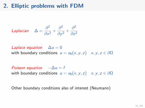
2. Elliptic problems with FDM
Laplacian ∆ =∂2
∂x2+
∂2
∂y2+
∂2
∂z2
Laplace equation ∆u = 0with boundary conditions u = u0(x , y , z) x , y , z ∈ ∂Ω
Poisson equation −∆u = fwith boundary conditions u = u0(x , y , z) x , y , z ∈ ∂Ω
Other boundary conditions also of interest (Neumann)
11 / 53

Elliptic problems Some applications
• Equilibrium problemsStructural analysis (strength of materials)Heat distribution
• Potential problemsPotential flow (inviscid, subsonic flow)Electromagnetics (fields, radiation)
• Eigenvalue problemsAcousticsMicrophysics
12 / 53

An elliptic model problem Poisson equation
∂2u
∂x2+∂2u
∂y2= f (x , y)
Computational domain Ω = [0, 1]× [0, 1] (unit square), Dirichletconditions u(x , y) = 0 on boundary
Uniform grid xi , yjN,Mi ,j=1 with equidistant mesh widths∆x = 1/(N + 1) and ∆y = 1/(M + 1)
Discretization Finite differences with ui ,j ≈ u(xi , yj)
ui−1,j − 2ui ,j + ui+1,j
∆x2+
ui ,j−1 − 2ui ,j + ui ,j+1
∆y2= f (xi , yj)
13 / 53
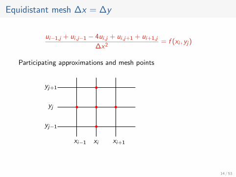
Equidistant mesh ∆x = ∆y
ui−1,j + ui ,j−1 − 4ui ,j + ui ,j+1 + ui+1,j
∆x2= f (xi , yj)
Participating approximations and mesh points
bababababa
xi−1 xi xi+1
yj
yj+1
yj−1
14 / 53

Computational stencil for ∆x = ∆y
ui−1,j + ui ,j−1 − 4ui ,j + ui ,j+1 + ui+1,j
∆x2= f (xi , yj)
“Five-point operator”
1
1 −4
1
1
15 / 53

The FDM linear system of equations
Lexicographic ordering of unknowns ⇒ block partitioned system
1
∆x2
T I 0 . . .I T I
I T I
. . . I. . . 0 I T
u·,1u·,2u·,3
...
u·,N
=
f (x·, y1)f (x·, y2)f (x·, y3)
...
f (x·, yN)
with Toeplitz matrix T = tridiag(1 −4 1)
The system is N2 × N2, hence large and very sparse
16 / 53

3. Elliptic problems with FEM
A general finite element method
Linear PDE Lu = fAnsatz u =
∑ciϕi ⇒ Lu =
∑ciLϕi
Requirement 〈ϕi , Lu − f 〉 = 0 gives coefficients ci
FEM is a least squares approximation, fitting a linear combinationof basis functions ϕi to the solution using orthogonality
Simplest case Piecewise linear basis functions 2nd order cG(1)
17 / 53
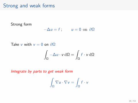
Strong and weak forms
Strong form−∆u = f ; u = 0 on ∂Ω
Take v with v = 0 on ∂Ω∫Ω−∆u · v dΩ =
∫Ωf · v dΩ
Integrate by parts to get weak form∫Ω∇u · ∇v =
∫Ωf · v
18 / 53
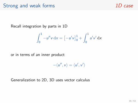
Strong and weak forms 1D case
Recall integration by parts in 1D∫ 1
0−u′′v dx =
[−u′v
]10
+
∫ 1
0u′v ′ dx
or in terms of an inner product
−〈u′′, v〉 = 〈u′, v ′〉
Generalization to 2D, 3D uses vector calculus
19 / 53

Weak form of −∆u = f ∆u = div(grad u)
Define inner product
〈v , u〉 =
∫Ωvu dΩ
and energy norm (note scalar product!)
a(v , u) = −∫
Ωv∆u dΩ =
∫Ω∇v · ∇u dΩ =
∫Ωgrad v · grad u dΩ
to get the weak form of −∆u = f as
a(v , u) = 〈v , f 〉
20 / 53
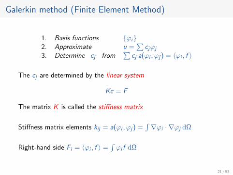
Galerkin method (Finite Element Method)
1. Basis functions ϕi2. Approximate u =
∑cjϕj
3. Determine cj from∑
cj a(ϕi , ϕj) = 〈ϕi , f 〉
The cj are determined by the linear system
Kc = F
The matrix K is called the stiffness matrix
Stiffness matrix elements kij = a(ϕi , ϕj) =∫∇ϕi · ∇ϕj dΩ
Right-hand side Fi = 〈ϕi , f 〉 =∫ϕi f dΩ
21 / 53
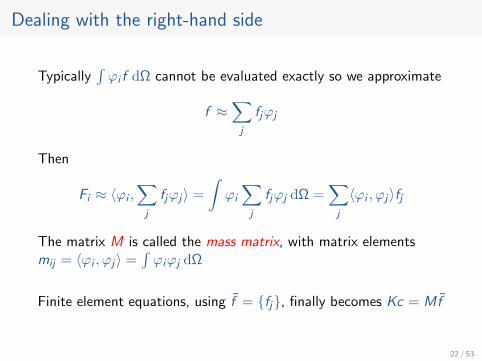
Dealing with the right-hand side
Typically∫ϕi f dΩ cannot be evaluated exactly so we approximate
f ≈∑j
fjϕj
Then
Fi ≈ 〈ϕi ,∑j
fjϕj〉 =
∫ϕi
∑j
fjϕj dΩ =∑j
〈ϕi , ϕj〉fj
The matrix M is called the mass matrix, with matrix elementsmij = 〈ϕi , ϕj〉 =
∫ϕiϕj dΩ
Finite element equations, using f = fj, finally becomes Kc = Mf
22 / 53

The FEM mesh cG(1) domain triangulation
Piecewise linear basis ϕj require domain triangulation
0 0.1 0.2 0.3 0.4 0.5 0.6 0.7 0.8 0.9 10
0.1
0.2
0.3
0.4
0.5
0.6
0.7
0.8
0.9
1
23 / 53

4. Parabolic problems Diffusion
The prototypical equation is the diffusion equation
ut = ∆u
Also nonlinear diffusion
ut = div (k(u) gradu)
Boundary and initial conditions are needed
Solution methods are now built by combining time-steppingmethods with space discretization of the Laplacian
24 / 53

Parabolic problems Some applications
• Diffusive processesHeat conduction ut = d · uxx
• Chemical reactionsReaction–diffusion ut = d · uxx + f (u)Convection–diffusion ut = ux + 1
Peuxx
• SeismologyParabolic waves ut = uux + d · uxx
Irreversibility ut = −∆u is not well-posed!
25 / 53

A parabolic model problem Diffusion
Equation ut = uxxInitial values u(0, x) = g(x)
Boundary values u(t, 0) = u(t, 1) = 0
Separation of variables u(t, x) := X (x)T (t) ⇒
ut = XT , uxx = X ′′T ⇒ T
T=
X ′′
X=: λ
T = Ceλt X = A sin√−λ x + B cos
√−λ x
26 / 53

Parabolic model problem. . .
Boundary values X (0) = X (1) = 0 ⇒ λk = −(kπ)2, therefore
Xk(x) =√
2 sin kπx Tk(t) = e−(kπ)2t
Fourier expansion of initial values g(x) =∑∞
1 ck√
2 sin kπx ⇒
Solution can be assembled
u(t, x) =√
2∞∑k=1
cke−(kπ)2tsin kπx
27 / 53

A.-M. Legendre and J. Fourier 1820
28 / 53

5. Method of lines (MOL) discretization
In ut = uxx , discretize ∂2/∂x2 by
uxx ≈ui−1 − 2ui + ui+1
∆x2
System of ODEs (semidiscretization) u = T∆xu reads
u =1
∆x2
−2 1
1 −2 1. . .
1 −2
u
29 / 53

Full FDM discretization
Note ui (t) ≈ u(t, xi ) along the line x = xi in the (t, x) plane
Using Explicit Euler time-stepping with uni ≈ u(tn, xi ) implies
un+1i − uni
∆t=
uni−1 − 2uni + uni+1
∆x2
With the Courant number µ = ∆t/∆x2 we obtain recursion
un+1i = uni + µ · (uni−1 − 2uni + uni+1)
30 / 53

Method of lines Computational stencil
Explicit Euler time stepping. Participating grid points
ba baba baxi−1 xi xi+1
tn
tn+1
Courant number µ = ∆t/∆x2
1
−µ 2µ − 1 −µ
31 / 53
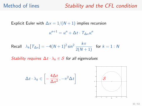
Method of lines Stability and the CFL condition
Explicit Euler with ∆x = 1/(N + 1) implies recursion
un+1· = un· + ∆t · T∆xu
n·
Recall λk [T∆x ] = −4(N + 1)2 sin2 kπ
2(N + 1)for k = 1 : N
Stability requires ∆t · λk ∈ S for all eigenvalues
−2.5 −2 −1.5 −1 −0.5 0 0.5−1.5
−1
−0.5
0
0.5
1
1.5
Re
Im
∆t · λk ∈[− 4∆t
∆x2,−π2∆t
]S
32 / 53
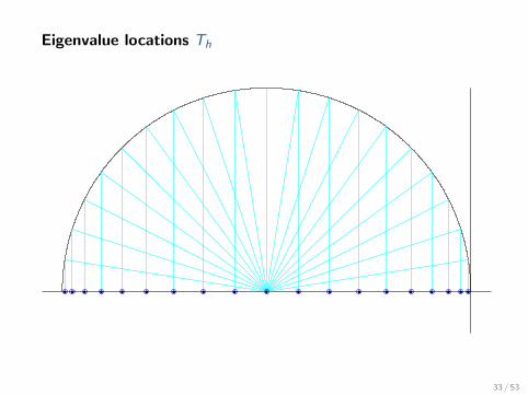
Eigenvalue locations Th
33 / 53

The CFL condition
For stability we need 4∆t/∆x2 ≤ 2
CFL condition (Courant, Friedrichs, Lewy 1928)
∆t
∆x2≤ 1
2
The CFL condition is a severe restriction on time step ∆t
Stiffness The CFL condition can be avoided by using A-stablemethods, e.g. Trapezoidal Rule or Implicit Euler
34 / 53

Experimental stability investigation
N = 30 internal pts in [0, 1], M = 187 time steps on [0, 0.1].Stable solution at CFL = .514
0
0.02
0.04
0.06
0.08
0.1
0
0.2
0.4
0.6
0.8
1
0
0.2
0.4
0.6
0.8
1
35 / 53
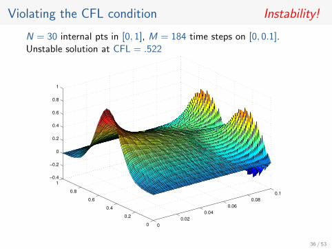
Violating the CFL condition Instability!
N = 30 internal pts in [0, 1], M = 184 time steps on [0, 0.1].Unstable solution at CFL = .522
0
0.02
0.04
0.06
0.08
0.1
0
0.2
0.4
0.6
0.8
1
−0.4
−0.2
0
0.2
0.4
0.6
0.8
1
36 / 53

Crank–Nicolson method (1947)
Crank–Nicolson method ⇔ Trapezoidal Rule for PDEs
The Trapezoidal Rule is
• implicit ⇒ more work/step• A–stable ⇒ no restriction on ∆t• Far more efficient
Theorem Crank–Nicolson is unconditionally stable
There is no CFL condition on the time-step ∆t which is why theCrank–Nicolson method is preferable
37 / 53

Crank–Nicolson method. . .
Courant number µ = ∆t/∆x2 ⇒ recursion
(I − µ
2T )un+1
· = (I +µ
2T )un·
with Toeplitz matrix T = tridiag(1 − 2 1)
Tridiagonal structure ⇒ low complexity
Refactorize only if Courant number µ = ∆t/∆x2 changes
38 / 53

6. Error analysis Convergence
MOL with explicit Euler for ut = uxx
Global error eni = uni − u(tn, xi )
Local error Insert exact solution to get
u(tn+1, xi )− u(tn, xi )
∆t=
u(tn, xi−1)− 2u(tn, xi ) + u(tn, xi+1)
∆x2− lni
Expand in Taylor series
−lni =∆t
2utt +
∆x2
12uxxxx + O(∆t2,∆x4)
39 / 53

The Lax Principle
Conclusion
Consistency lni → 0 as ∆t,∆x → 0Stability CFL condition ∆t/∆x2 ≤ 1/2
Convergence eni → 0 as ∆t,∆x → 0
Theorem (Lax Principle)
Consistency + Stability ⇒ Convergence
Note Choice of norm is very important
40 / 53

Convergence order
With local error
−lni =∆t
2utt +
∆x2
12uxxxx = O(∆t,∆x2)
and stability in terms of CFL condition µ = ∆t/∆x2 ≤ 1/2 wehave global error eni = O(∆t,∆x2)
For fixed µ we have ∆t ∼ ∆x2 and it follows that
Global error eni = O(∆t,∆x2) = O(∆x2) ⇒
Theorem The order of convergence is p = 2
41 / 53
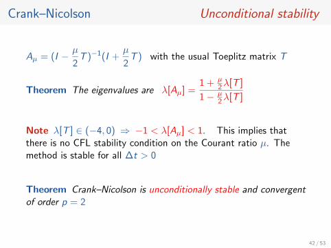
Crank–Nicolson Unconditional stability
Aµ = (I − µ
2T )−1(I +
µ
2T ) with the usual Toeplitz matrix T
Theorem The eigenvalues are λ[Aµ] =1 + µ
2λ[T ]
1− µ2λ[T ]
Note λ[T ] ∈ (−4, 0) ⇒ −1 < λ[Aµ] < 1. This implies thatthere is no CFL stability condition on the Courant ratio µ. Themethod is stable for all ∆t > 0
Theorem Crank–Nicolson is unconditionally stable and convergentof order p = 2
42 / 53

Experimental stability investigation
N = 30 internal pts in [0, 1], M = 30 time steps on [0, 0.1] Stablesolution at CFL = 3.2
0
0.02
0.04
0.06
0.08
0.1
0
0.2
0.4
0.6
0.8
1
0
0.2
0.4
0.6
0.8
1
43 / 53

Convection–diffusion ut = uxx + αux − f
Space operator with homogeneous Dirichlet conditions on [0, 1]
Lαu = u′′ + αu′
Convection dominated for Peclet numbers |α| 1, with boundarylayer at x = 1 for α < 0
Lα is not self-adjoint, but it is equi-elliptic wrt Peclet number
λk [Lα] = −(kπ)2 − α2
4
uk(x) = e−αx/2 sin kπx
44 / 53
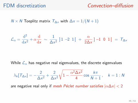
FDM discretization Convection–diffusion
N × N Toeplitz matrix T∆x with ∆x = 1/(N + 1)
Lα =d2
dx2+ α
d
dx∼ 1
∆x2] 1 −2 1 [ +
α
2∆x]−1 0 1 [ = T∆x
While Lα has negative real eigenvalues, the discrete eigenvalues
λk [T∆x ] = − 2
∆x2+
2
∆x2
√1− α2∆x2
4cos
kπ
N + 1, k = 1 : N
are negative real only if mesh Peclet number satisfies |α∆x | < 2
45 / 53

7. Parabolic problems with cG(1) FEM
Consider diffusion problem in strong form ut − uxx = 0 withDirichlet boundary conditions
Multiply by test function v and integrate by parts∫ 1
0vut dx +
∫ 1
0v ′u′ dx = 0
In terms of inner product and energy norm –
Weak form 〈v , ut〉+ a(v , u) = 0 for all v with v(0) = v(1) = 0
46 / 53

Galerkin cG(1) FEM for parabolic equations
1. Basis functions ϕi2. Approximate u(t, x) =
∑cj(t)ϕj(x)
3. Determine cj from 〈ϕi , ut〉+ a(ϕi , u) = 0
Note 〈ϕi , ut〉 =∑
cj〈ϕi , ϕj〉 and a(ϕi , u) =∑
cj〈ϕ′i , ϕ′j〉
We get an initial value problem
M∆x c + K∆xc = 0
for the determination of the coefficients cj(t) with c(0) determinedby the initial condition
47 / 53
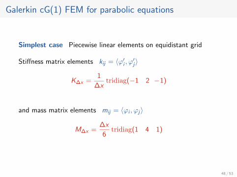
Galerkin cG(1) FEM for parabolic equations
Simplest case Piecewise linear elements on equidistant grid
Stiffness matrix elements kij = 〈ϕ′i , ϕ′j〉
K∆x =1
∆xtridiag(−1 2 −1)
and mass matrix elements mij = 〈ϕi , ϕj〉
M∆x =∆x
6tridiag(1 4 1)
48 / 53

Galerkin cG(1) FEM for parabolic equations. . .
Note that in the initial value problem
M∆x c + K∆xc = 0
the matrix M∆x is tridiagonal ⇒ no advantage from explicittime stepping methods
Explicit Euler
M∆x(cn+1 − cn) = −∆t · K∆xcn
requires the solution of a tridiagonal system on every step
49 / 53
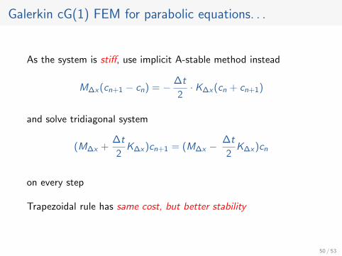
Galerkin cG(1) FEM for parabolic equations. . .
As the system is stiff, use implicit A-stable method instead
M∆x(cn+1 − cn) = − ∆t
2· K∆x(cn + cn+1)
and solve tridiagonal system
(M∆x +∆t
2K∆x)cn+1 = (M∆x −
∆t
2K∆x)cn
on every step
Trapezoidal rule has same cost, but better stability
50 / 53

8. Well-posedness
Linear partial differential equation
ut = Lu + f , 0 ≤ x ≤ 1, t ≥ 0, u(0, x) = h(x),
u(t, 0) = φ0(t), u(t, 1) = φ1(t)
Suppose
wt = Lw + f , w(0, x) = h(x)vt = Lv + f , v(0, x) = h(x) + g(x)
Subtract to get homogeneous Dirichlet problem
ut = Lu, u(0, x) = g(x), φ0(t) ≡ 0, φ1(t) ≡ 0
51 / 53

Well-posedness Time evolution
Suppose time evolution u(t, x) = E(t)g(x)
Definition The equation is well-posed if for every t∗ > 0 there isa constant 0 < C (t∗) <∞ such that ‖E(t)‖ ≤ C (t∗) for all0 ≤ t ≤ t∗
Definition A well-posed equation has a solution that
• depends continuously on the initial value (the “data”)
• is uniformly bounded in any compact interval
52 / 53

ut = uxx is well posed
Fourier series expansion g(x) =√
2∑∞
1 ck sin kπx implies
u(t, x) =√
2∞∑k=1
cke−(kπ)2t sin kπx
‖E(t)g‖22 =
∫ 1
0|u(t, x)|2 dx
= 2∞∑k=1
∞∑j=1
ckcje−(k2+j2)π2t
∫ 1
0sin kπx sin jπx dx
=∞∑k=1
c2k e−2(kπ)2t ≤
∞∑k=1
c2k = ‖g‖2
2
Hence ‖E(t)‖2 ≤ 1 for every t ≥ 0
53 / 53


