Numerical Methods for (Time-Dependent) HJ PDEs · · 2012-12-06Numerical Methods for...

Numerical Methods for (Time-Dependent) HJ PDEs

Ian MitchellDepartment of Computer ScienceThe University of British Columbia

research supported byNational Science and Engineering Research Council of Canada

March 2008 Ian Mitchell (UBC Computer Science) 2

Outline• Basic representation and approximation of functions

which solve evolutionary PDEs– Shocks / kinks for HJ PDEs

• Level Set Toolbox, alternative software and schemes• Convergence, consistency, stability & monotonicity• Terminology from level set methods• Example: approximating the identical vehicle collision

avoidance reach tube


Representing a Continuous Function

• Computer representations must be finite– Consequently, we are forced to construct a discrete, finite

representation of ψψψψ: “discretization”

• Combination of basis functions

– If ηηηηjjjj are trigonometric, we get spectral methods– If ηηηηjjjj have local support, we get finite element (FE) methods

• Create grid of state space, store value of ψψψψ at the nodes– Called finite difference (FD) because of derivative approximation

• Create grid of state space, store average nearby value of ψψψψ– Called finite volume (FV), uncommon outside fluid mechanics


Solving an Evolution PDE

• Although we can represent a time dependent function φφφφ as a function in Rdddd+1, most often it is represented as a collection of functions in Rdddd at a set of time instants

• Much of the literature for (time-dependent) HJ PDEs grew out of conservation law schemes, so there is shared terminology

• In a Lagrangian approach, the function representation moves with the underlying flow

• In an Eulerian approach, the function representation does not move with the underlying flow– It is often fixed, but may be adaptive

– Updates are done without following the underlying flow

• In a semi-Lagrangian approach, the underlying flow is used to update a fixed representation


Pros and Cons• Lagrangian

– Easy concentration of resources in regions of high complexity, but other regions may become sparse

– Challenging to collect topological information, detect shocks

• Eulerian– Easy to collect topological information and detect shocks but

challenging to adapt representation in regions of high complexity

– CFL timestep restrictions may slow computations

• Semi-Lagrangian– Mapping between Eulerian and Lagrangian representations

causes loss of accuracy due to interpolation


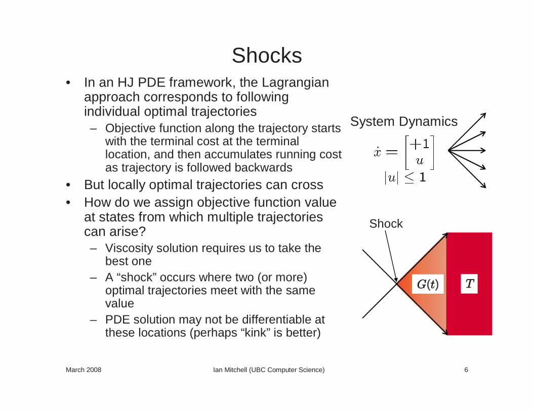
Shocks• In an HJ PDE framework, the Lagrangian

approach corresponds to following individual optimal trajectories– Objective function along the trajectory starts

with the terminal cost at the terminal location, and then accumulates running cost as trajectory is followed backwards

• But locally optimal trajectories can cross• How do we assign objective function value

at states from which multiple trajectories can arise?– Viscosity solution requires us to take the

best one– A “shock” occurs where two (or more)

optimal trajectories meet with the same value

– PDE solution may not be differentiable at these locations (perhaps “kink” is better)

System Dynamics

Shock

TTTTGGGG(tttt)







Level Set Methods• Adopts Eulerian approach because of the shock detection

problem

• Originally designed for dynamic implicit surface evolution– Representing the moving surface of a fluid

– Merging and pinch-off handled automatically

• Easy to implement– Finite difference representation and approximation– Dimension by dimension treatment of spatial terms– Method of lines treatment of temporal terms

• Borrows extensively from conservation laws– Schemes with high orders of accuracy

• Tries to avoid complications of boundary conditions– Reinitialization procedure for implicit surfaces

• Implementation available: Toolbox of Level Set Methods


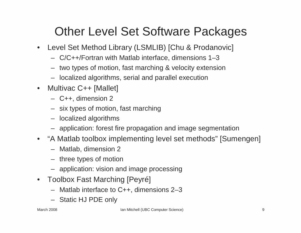
Other Level Set Software Packages• Level Set Method Library (LSMLIB) [Chu & Prodanovic]

– C/C++/Fortran with Matlab interface, dimensions 1–3

– two types of motion, fast marching & velocity extension– localized algorithms, serial and parallel execution

• Multivac C++ [Mallet]– C++, dimension 2

– six types of motion, fast marching– localized algorithms– application: forest fire propagation and image segmentation

• “A Matlab toolbox implementing level set methods” [Sumengen]– Matlab, dimension 2

– three types of motion– application: vision and image processing

• Toolbox Fast Marching [Peyré]– Matlab interface to C++, dimensions 2–3– Static HJ PDE only


Alternatives• Semi-Lagrangian schemes

– Falcone, Ferretti, Soravia…

• Viability schemes– Saint-Pierre

• Many reachability algorithms unrelated to PDEs


Convergence and Related Concepts• Since we cannot solve the PDE exactly, we would like that our

approximation approaches the true solution as some refinement parameter goes to zero: “convergence”– For our representation, xxxx 0 and tttt 0

• Convergence can be challenging to prove directly

• For linear PDEs, consistency + stability implies convergence– HJ PDE is not linear, but Barles & Souganidis (1991) showed that

consistency + stability + monotonicity implies convergence

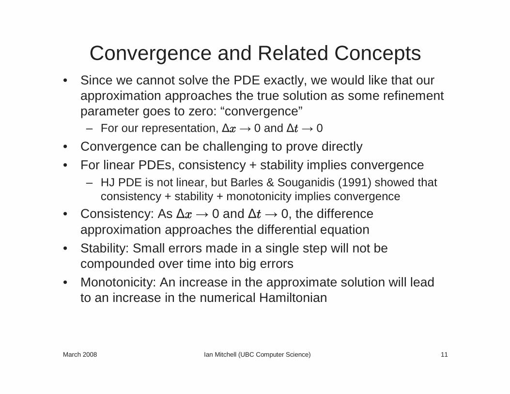
• Consistency: As xxxx 0 and tttt 0, the difference approximation approaches the differential equation

• Stability: Small errors made in a single step will not be compounded over time into big errors

• Monotonicity: An increase in the approximate solution will lead to an increase in the numerical Hamiltonian







Method of Lines

• One method for dealing with evolution equations that have both spatial and temporal derivatives

• Basic idea: discretize and approximate spatial terms to form a coupled set of ordinary differential equations in time

– For example

– Now solve ODE in time for φφφφ(xxxxiiii, tttt) for all nodes xxxxiiii


CFL Condition• In the simplest approaches to solving the

temporal ODE (explicit schemes) require a restriction on the temporal discretization ∆ttttwith respect to the spatial discretization ∆xxxx– Intuitively the restriction corresponds to

restricting ∆tttt such that trajectories of the underlying dynamics will not cross more than ∆xxxx in time ∆tttt

– For deterministic systems, ∆t t t t = O(∆xxxx)

– The constant is related to the velocity of the underlying dynamics: the faster the flow, the smaller ∆tttt

– Mathematically, the restriction arises from stability

xxxx

tttt

xxxx – ∆xxxx xxxx + ∆xxxx

tttt + ∆tttt

CFL satisfied

xxxx

tttt

xxxx – ∆xxxx xxxx + ∆xxxx

tttt + ∆tttt

CFL failed


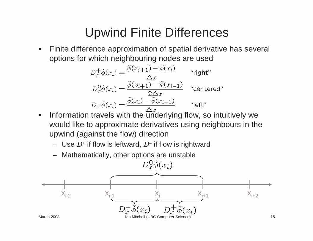
Upwind Finite Differences• Finite difference approximation of spatial derivative has several

options for which neighbouring nodes are used

• Information travels with the underlying flow, so intuitively we would like to approximate derivatives using neighbours in the upwind (against the flow) direction– Use DDDD+ if flow is leftward, DDDD– if flow is rightward

– Mathematically, other options are unstable

xixi-2 xi-1 xi+1 xi+2


ENO / WENO• Standard schemes for higher orders of accuracy require

underlying function φφφφ to have (more) derivatives– Attempts to approximate functions without those derivatives lead to

incorrect oscillatory approximations

• Since φφφφ may have places without derivatives, Essentially Non-Oscillatory schemes build multiple approximations, and chose the least oscillatory– Extension to Weighted ENO combines all approximations with

weights that favour least oscillatory approximation near a kink, but in smooth regions achieve even higher order of accuracy

• Not monotonic, so no convergence theory– Work very well in practice

xixi-3 xi-2 xi-1 xi+1 xi+2 xi+3


Numerical Hamiltonian

• Obvious substitution is unstable

• Simplest approximation: Lax-Friedrichs– used in Crandall & Lions (1984)

– Essentially adds dissipation

• Upwinding: for HHHH(xxxx,pppp) = pppp · ffff(xxxx)

– There may not be a single consistent “upwind” direction when the dynamics have inputs


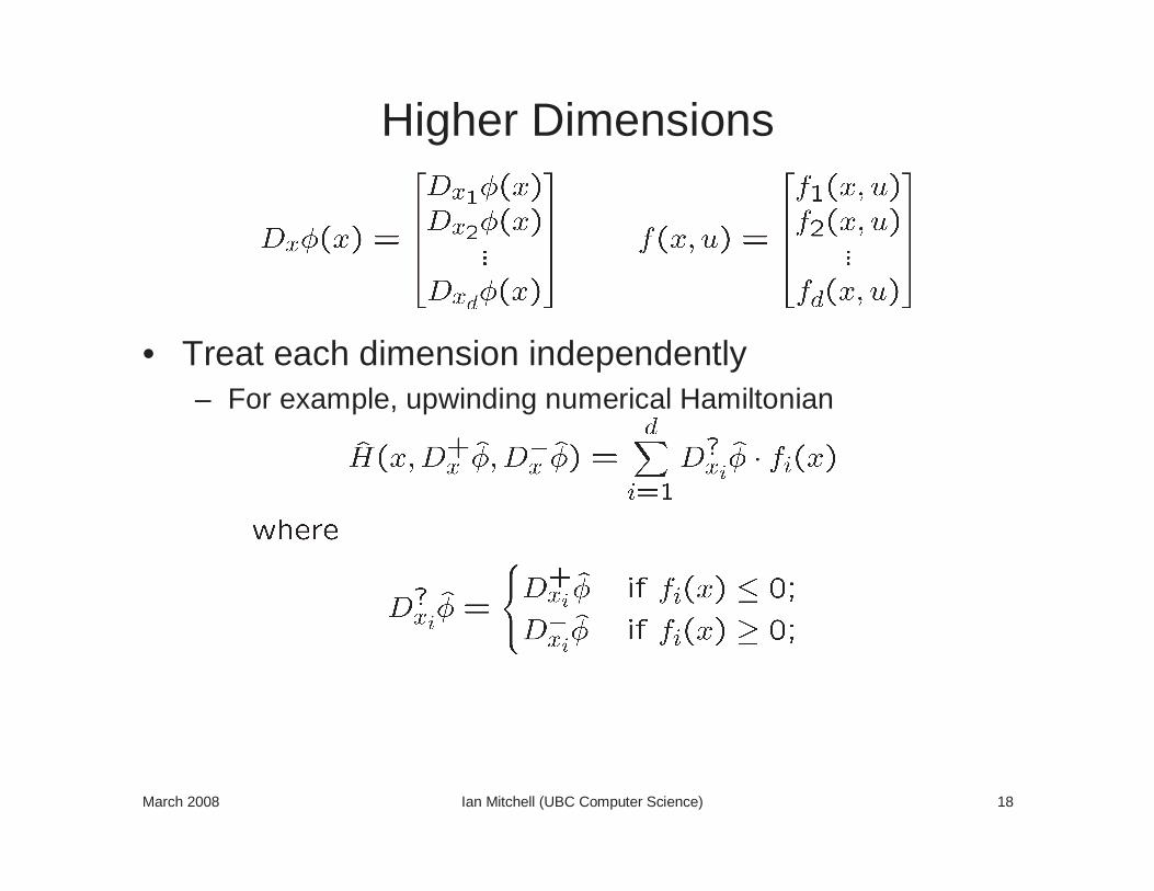
Higher Dimensions

• Treat each dimension independently– For example, upwinding numerical Hamiltonian


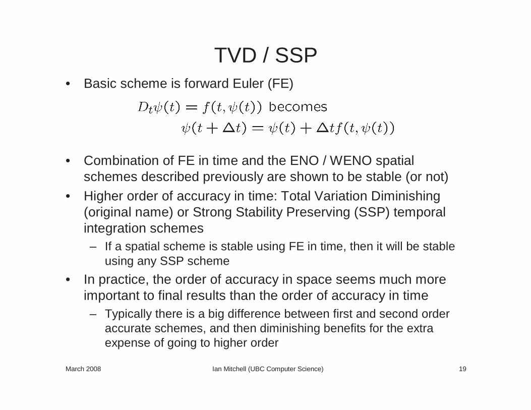
TVD / SSP• Basic scheme is forward Euler (FE)

• Combination of FE in time and the ENO / WENO spatial schemes described previously are shown to be stable (or not)

• Higher order of accuracy in time: Total Variation Diminishing (original name) or Strong Stability Preserving (SSP) temporal integration schemes– If a spatial scheme is stable using FE in time, then it will be stable

using any SSP scheme

• In practice, the order of accuracy in space seems much more important to final results than the order of accuracy in time– Typically there is a big difference between first and second order

accurate schemes, and then diminishing benefits for the extra expense of going to higher order


Implicit Surface Reinitialization• Restriction of implicit surface function to signed distance often

produces a more accurate representation– Gradient magnitude is not too small or too large, so location of and

normal to the surface is easy to estimate

• Evolution of surface may perturb signed distance– Converging or diverging flow– Non-physical boundary conditions

• However, value of implicit surface function away from zero levelset does not matter

• Reinitialization rebuilds a signed distance function from an implicit surface function without changing the zero level set

• Several available schemes– Fast marching (uses auxiliary static HJ PDE)– Reinitialization equation (uses auxiliary time-dependent HJ PDE)– Toolbox supports the latter but not the former


Reducing the Cost of Level Set Methods• Solve Hamilton-Jacobi equation only in a band near interface

• Computational challenge: handling stencils near edge of band– “Narrowbanding” uses low order accurate reconstruction whenever

errors are detected

– “Local level set” modifies Hamiltonian near edge of band

• Data structure challenge: handling merging and breaking of interface

• Not supported in the Toolbox


Implementing Reach Tubes• Collision avoidance example from the Toolbox

– See Toolbox documentation section 2.6

• Pitfalls to avoid– Failure to include the kernel directories in the Matlab path

– Grid is too coarse

– State space dimensions are poorly scaled (be careful to scale both grid and dynamics)

– Boundary conditions are incorrect– Incorrect initialization and/or incorrect grid bounds

– Numerical instability caused by buggy boundary conditions, too little dissipation in Lax-Friedrichs, poor dimensional scaling, too large CFL, etc.

– Mixing up ndgrid and meshgrid based grids (see documentation for discussion)

Numerical Methods for (Time-Dependent) HJ PDEs

For more information contact

Ian MitchellDepartment of Computer ScienceThe University of British Columbia

[email protected]

http://www.cs.ubc.ca/~mitchell

Date post:	25-May-2018
Category:	Documents
Upload:	phamkien
View:	219 times
Download:	0 times

Numerical Methods for (Time-Dependent) HJ PDEs · · 2012-12-06Numerical Methods for...

Documents