Numerical Methods for Turbomachinery Aeromechanical ...457544/FULLTEXT01.pdf · Numerical Methods...

Numerical Methods for Turbomachinery Aeromechanical Predictions

María Angélica Mayorca

Doctoral Thesis 2011

Department of Energy Technology School of Industrial Engineering and Management

Royal Institute of Technology Stockholm, Sweden

ISBN 978-91-7501-135-6 TRITA KRV Report 11/08 ISSN 1100/7990 ISRN KTH/KRV/11/08-SE © María Mayorca

Doctoral Thesis / María Mayorca Page 1

ABSTRACT

In both aviation and power generation, gas turbines are used as key components. An important driver of technological advance in gas turbines is the race towards environmentally friendly machines, decreasing the fuel burn, community noise and NOx emissions. Engine modifications that lead to propulsion efficiency improvements whilst maintaining minimum weight have led to having fewer stages and lower blade counts, reduced distance between blade rows, thinner and lighter components, highly three dimensional blade designs and the introduction of integrally bladed disks (blisks). These changes result in increasing challenges concerning the structural integrity of the engine. In particular for blisks, the absence of friction at the blade to disk connections decreases dramatically the damping sources, resulting in designs that rely mainly on aerodynamic damping. On the other hand, new open rotor concepts result in low blade-to-air mass ratios, increasing the influence of the surrounding flow on the vibration response.

This work presents the development and validation of a numerical tool for aeromechanical analysis of turbomachinery (AROMA - Aeroelastic Reduced Order Modeling Analyses), here applied to an industrial transonic compressor blisk. The tool is based on the integration of results from external Computational Fluid Dynamics (CFD) and Finite Element (FE) solvers with mistuning considerations, having as final outputs the stability curve (flutter analysis) and the fatigue risk (forced response analysis). The first part of the study aims at tracking different uncertainties along the numerical aeromechanical prediction chain. The amplitude predictions at two inlet guide vane setups are compared with experimental tip timing data. The analysis considers aerodynamic damping and forcing from 3D unsteady Navier Stokes solvers. Furthermore, in-vacuo mistuning analyses using Reduced Order Modeling (ROM) are performed in order to determine the maximum amplitude magnification expected. Results show that the largest uncertainties are from the unsteady aerodynamics predictions, in which the aerodynamic damping and forcing estimations are most critical. On the other hand, the structural dynamic models seem to capture well the vibration response and mistuning effects.

The second part of the study proposes a new method for aerodynamically coupled analysis: the Multimode Least Square (MLS) method. It is based on the generation of distributed aerodynamic matrices that can represent the aeroelastic behavior of different mode-families. The matrices are produced from blade motion unsteady forces at different mode-shapes fitted in terms of least square approximations. In this sense, tuned or mistuned interacting mode families can be represented. In order to reduce the domain size, a static condensation technique is implemented. This type of model permits forced response prediction including the effects of mistuning on both the aerodynamic damping as well as on the structural mode localization. A key feature of the model is that it opens up for considerations of responding mode-shapes different to the in-vacuo ones and allows aeroelastic predictions over a wide frequency range, suitable for new design concepts and parametric studies.

Keywords: aeromechanics, turbomachinery, mistuning, ROM, CFD, FEM, blisk, methods

Page 2 Doctoral Thesis / María Mayorca


SAMMANFATTNING

Både inom flyg- och kraftgenreringsindustrin används gasturbiner som huvudkomponenter. En viktig drivkraft i den tekniska utvecklingen av gas turbiner är strävan mot mer miljövänliga maskiner, genom att minska bränslekonsumtion, buller och skadliga utsläpp av NOx. En förbättring av verkningsgraden under förutsättningen att vikten hålls oförändrad eller till och med minskad, har lett till andra viktiga modifikationer: reducerat antal steg och färre skovlar per steg, minskat axiellt avstånd mellan bladgitter, smalare och lättare komponenter, aggressiv 3D bladdesign och introducering av bladintegrerade rotorskivor (blisk). Alla dessa ändringar resulterar i en omprövning för motors strukturella integritet. Detta är särskilt viktigt för ”blisk”, där en total frånvaro av friktionsdämpning mellan bladen och skivan leder till att dämpningen i systemet huvudsakligen består av den aerodynamiska dämpningen. Å andra sidan, det nya öppna-rotor konceptet har lett till ett lågt blad-mot-luft massförhållande vilket i sin tur har orsakat en ökad inverkan av flödet på strukturens vibratoriska egenskaper.

Den här avhandlingen beskriver utvecklingen och valideringen av det numeriska verktyget för aeromekanisk analys av turbomaskiner (AROMA - Aeroelastic Reduced Order Model Analysis), och dess tillämpning i analys av en industriell transonisk kompressor –’blisk’. Verktyget hanterar resultat från externa CFD och FE koder, och tar hänsyn till asymmetrier (mistuning) genom att tillämpa Reduced Order Modelling (ROM). Som slutresultat fås stabilitetskurvor (fladder analys) eller en uppskattning av risken för utmattning (vibratorisk respons analys). Den första delen av studien fokuserar på att spåra möjliga felkällor i predikteringsproceduren av HCF. De numeriska resultaten för två olika inställningar av inlopps ledskenor jämförs med experimentell data från ”tip-timing”-tester genomförda på den transoniska kompressorn. Analysen omfattar prediktering av aerodynamisk dämpning och aerodynamisk excitation från 3D Navier Stokes. Därefter genomfördes en ROM mistuning analys i vacuum för att kunna bestämma den förväntade maximala amplitudförhöjningen och jämföra denna med det uppmätta värdet. Resultaten visar att den största osäkerheten kommer från prediktering av instationär aerodynamik, i vilken uppskattningen av aerodynamisk dämpning och aerodynamisk excitation har betydande påverkan. Det påvisas dock här att den strukturdynamiska modellen som används verkar fånga det vibratoriska respons beteendet och påverkan av mistuning med rimlig noggrannhet.

I den senare delen av studien föreslås en ny metod för en aerodynamisk kopplad analys: Multimode Least Square (MLS) method. Metoden baseras på generering av distribuerade aerodynamiska matriser som kan beskriva aeroelastiskt beteende hos olika modfamiljer. Matriser genereras från instationära krafter orsakade av bladrörelse i olika oscillationsmoder, som approximeras med minsta kvadrat metoden. På det här viset, kan både symmetriska och osymmetriska modfamiljer beskrivas. För att minska storleken på domänen, har en reduceringsmetod baserad implementerats. Den här typen av modell tillåter prediktering av vibratorisk respons på ett väldigt generellt sätt där effekter av mistuning på både aerodynamisk dämpning och på strukturell modlokalisering tas i beaktande. Huvudegenskapen för modellen är att den öppnar för analys av svarande oscillationsmoder som är olika dom vakuum-bestämda moderna. Dessutom, tillåter modellen en aeroelastisk prediktering i ett brett frekvensområde, passande för nya konstruktioner och parameterstudier.

Nyckelord: aeromekanisk konstruktion, turbomaskiner, numeriskt verktyg, ROM, CFD, FEM, metoder, blisk, mistuning



PREFACE

The present work is based is built on five publications, whereof the first three were included in a licentiate thesis [Mayorca, 2010]. Licentiate Thesis Mayorca M., 2010 “Development and Validation of a Numerical Tool for the Aeromechanical Design of Turbomachinery” Licentiate Thesis in Energy Technology, Royal Institute of Technology. Stockhom, Sweden ISBN 978-91-7415-561-7

Paper I Mayorca M. A., De Andrade J., Vogt D. M., Mårtensson H., Fransson T. H., 2011 “Effect of Scaling of Blade Row Sectors on the Prediction of Aerodynamic Forcing in a Highly-Loaded Transonic Compressor Stage” Journal of Turbomachinery, Vol. 133(2), 021013. doi: 10.1115/1.4000579

Paper II Mayorca M. A., Vogt D. M., Mårtensson H., Fransson T. H., 2009 "Numerical Tool for Prediction of Aeromechanical Phenomena in Gas Turbines" ISABE-2009-1250 Paper presented at the 19th ISABE Conference in Montreal, Canada

Paper III Mayorca M. A., Vogt D. M., Mårtensson H., Fransson T. H., 2010 "A New Reduced Order Modeling for Stability and Forced Response Analysis of Aero-Coupled Blades Considering Various Mode Families" ASME Paper GT2010-22745* *Accepted for Publication in the Journal of Turbomachinery

Paper IV Mayorca M. A., Vogt D. M., Mårtensson H., Fransson T. H., 2011 “Prediction of Turbomachinery Aeroelastic Behavior from a Set of Representative Modes” ASME Paper GT2011-46690* *Accepted for Publication in the Journal of Turbomachinery

Paper V Mayorca M. A., Vogt D. M., Andersson C., Mårtensson H., Fransson T. H., 2012 "Uncertainty of Forced Response Numerical Predictions of an Industrial Blisk - Comparison with Experiments" ASME Paper GT2012-69534* *To be published in ASME Turbo Expo 2012


The involvement of Dr. Damian Vogt and Prof. Torsten Fransson in the above publications consisted of problem formulation and discussion of results. Mr. Hans Mårtensson was involved in problem formulation, methodology and results discussions giving an industrial perspective. The involvement of M.Sc. Jesús De Andrade in Paper I consisted of supervised computations for M.Sc. thesis. The Participation of Dr. Clas Andersson in Paper V consisted of experimental data acquisition. For all publications the underlying material was part of the work elaborated in this thesis.


ACKNOWLEDGEMENT

To Prof. Torsten Fransson, Chair of Heat and Power Technology at KTH, for giving me the opportunity to perform this work and for always sharing his views and opening new doors. To Damian Vogt at KTH, I would like to express my endless gratitude for his guidance, positive and motivating thoughts, his priceless time and enthusiastic support during the whole path towards this work. To Hans Mårtensson at Volvo Aero, Trollhättan, for sharing his bright ideas and giving valuable feedback. His positive spirit on the project meetings made the working environment much more fun. To all the TurboVib members from Volvo Aero, Siemens Industrial Turbomachinery AB and KTH, Sweden, for their support and fruitful discussions. It was much easier advancing on the research projects by working together as a team. To my colleagues at KTH for their company, support, good discussions and all the nice coffee breaks. Special thanks are directed to my family: my Mom Doris, my Dad Gonzalo and my sisters María Alicia and María Alejandra Mayorca for their unconditional love and support even over distance. To my friends in Sweden, for becoming my second family and being there for the good and tough moments. To my friends at home for still being there after time and distance. To my dear Carlos, for supporting me in important moments of this journey with love and patience. The present study has been promoted by the Swedish Defense Procurement Agency (FMV) to the development and research in compressors. The research has been funded by the Swedish Energy Agency, Siemens Industrial Turbomachinery AB and Volvo Aero Corporation through the Swedish research program TURBO POWER, the support of which is gratefully acknowledged.



CONTENT

Abstract ................................................................................................................................ 1

Sammanfattning ................................................................................................................... 3

Preface ................................................................................................................................ 5

Acknowledgement ............................................................................................................... 7

Content ................................................................................................................................ 9

List of Figures .................................................................................................................... 12

Nomenclature .................................................................................................................... 15

1. Background ................................................................................................................ 19

1.1. Gas Turbines ....................................................................................................... 19

1.2. Aeromechanical Problems ................................................................................... 21 1.2.1. Forced Response ......................................................................................... 22 1.2.2. Stability and Aerodynamic Damping ............................................................. 31 1.2.3. Mistuning ...................................................................................................... 35

2. State of the Art in Aeromechanics of Turbomachinery ................................................ 39

2.1. Aeromechanical Design ....................................................................................... 39 2.1.1. Fluid Dynamic Unsteady Calculation Models ............................................... 40 2.1.2. Structural Models ......................................................................................... 41 2.1.3. Fluid-structure Coupling ............................................................................... 43

2.2. Accuracy in HCF predictions ............................................................................... 45

3. Objectives and Approach ............................................................................................ 47

3.1. Objectives ............................................................................................................ 47

3.2. Approach ............................................................................................................. 47

4. Aeroelastic Reduced Order Modeling Analyses (AROMA) ......................................... 51

4.1. AROMA Philosophy ............................................................................................. 51

4.2. AROMA Structure ................................................................................................ 51

4.3. Limitations ........................................................................................................... 53

4.4. Governing Equations ........................................................................................... 54 4.4.1. Forced Response ......................................................................................... 54


4.4.2. Aerodynamic Damping – Single Degree of Freedom Approach ................... 54 4.4.3. Multimode Least Square Method (MLS) ....................................................... 56 4.4.4. MLS Application to Arbitrary Modes ............................................................. 58 4.4.5. Guyan Reduction .......................................................................................... 60

5. AROMA Validation ...................................................................................................... 63

5.1. Tuned Analysis .................................................................................................... 63

5.2. Mistuned Analysis ................................................................................................ 64

5.3. ROM Mistuned Forced Response ....................................................................... 65

6. Test Case Description ................................................................................................ 69

7. Quantification Of Numerical Uncertanties ................................................................... 71

7.1. Scaling of Blade Row Sectors Accuracy .............................................................. 71 7.1.1. Scaling Factors ............................................................................................. 71 7.1.2. Scaled Cases ............................................................................................... 72 7.1.3. Generalized Forces Calculation ................................................................... 73 7.1.4. Scaling Accuracy .......................................................................................... 73

7.2. CFD-FE Mapping Uncertainty.............................................................................. 76 7.2.1. Fluid and Structure Domains ........................................................................ 76 7.2.2. Harmonic Forces to Structural Mesh ............................................................ 77 7.2.3. Mode-shape Mapped to the Fluid Domain ................................................... 78 7.2.4. Mapping Method Difference ......................................................................... 78

7.3. ROM Convergence Study .................................................................................... 79 7.3.1. Master Nodes Selection ............................................................................... 79 7.3.2. Accuracy of Guyan Reduction ...................................................................... 80

8. Forced Response Prediction and Comparison with Experimental Data ..................... 85

8.1.1. Tip Timing Data Acquisition Description ....................................................... 85 8.1.2. Frequency Analysis ...................................................................................... 87 8.1.3. Steady State Calculation .............................................................................. 89 8.1.4. Unsteady Blade Row Interaction .................................................................. 90 8.1.5. Potential and Viscous Effects ....................................................................... 92 8.1.6. Aerodynamic Damping ................................................................................. 95 8.1.7. In-vacuo Mistuning Analysis ......................................................................... 99 8.1.8. Vibration Response Prediction ................................................................... 100 8.1.9. Summary of Uncertainties Contributors ...................................................... 103

9. Multimode Least Square Method (MLS) ................................................................... 105

9.1. Stability and Forced Response of Tuned and Mistuned Cases ......................... 105 9.1.1. Validation with the Single Degree of Freedom Approach ........................... 105 9.1.2. Tuned Forced Response ............................................................................ 107 9.1.3. Mistuned Forced Response ........................................................................ 108

9.2. Aeroelastic Behavior from Arbitrary Modes ....................................................... 110 9.2.1. Reference Case ......................................................................................... 110


9.2.2. Guyan Arbitrary Modes (GAMs) ................................................................. 112 9.2.3. Frequency Fit Considerations ..................................................................... 114 9.2.4. Influence Coefficients Fit ............................................................................ 115 9.2.5. Aerodynamic Damping Prediction by GAMs ............................................... 116

10. Conclusions .......................................................................................................... 119

11. References ............................................................................................................ 121


LIST OF FIGURES

Figure 1-1: a) Modern Civil Aircraft Gas Turbine GEnx; b) Carbon Fiber Composite Fan blade with Titanium Edge; c) Compressor blisks (Courtesy of General Electric Aviation) ...................................................................................................................... 19

Figure 1-2: Increase of OPR for commercial engines over the years. (Kestner et al. 2011) ................................................................................................................................... 20

Figure 1-3: Failed compressor blisk in the CT7-9B engine due to HCF (Australian Transport Safety Bureau, 2010) ................................................................................. 21

Figure 1-4: Haigh Diagram (sines) .................................................................................... 22 Figure 1-5: Beam mode-shapes and nomenclature .......................................................... 24 Figure 1-6: Disk mode-shapes and nomenclature ............................................................ 24 Figure 1-7: Holografic images of a shrouded fan [Mickolajczak et al., 1975] .................... 24 Figure 1-8: Free response of a bladed disk. Nodal diameter vs. eigen-frequency vs.

rotational speed .......................................................................................................... 26 Figure 1-9: Campbell Diagram Illustration ......................................................................... 27 Figure 1-10: ZZENF diagram; Engine Order (EO) resonance crossings and nodal

diameter pattern; operating range speed indicated (squares); resonance crossings (stars) ......................................................................................................................... 27

Figure 1-11: Illustration of the blade row interaction mechanisms .................................... 29 Figure 1-12: Vibration amplitude increase due to flutter in transonic compressor blades

cascade; different reduced frequencies; (Belz and Hennings 2006) ........................... 32 Figure 1-13: Stability Curve Illustration ............................................................................. 33 Figure 1-14: Illustration of a lumped mass-spring system with only aerodynamic coupling

................................................................................................................................... 34 Figure 1-15: Aerodynamic damping change due to increase in frequency mistuning

[Martel et al. 2008] ...................................................................................................... 37 Figure 2-1: Aeromechanical design chain including forced response and stability

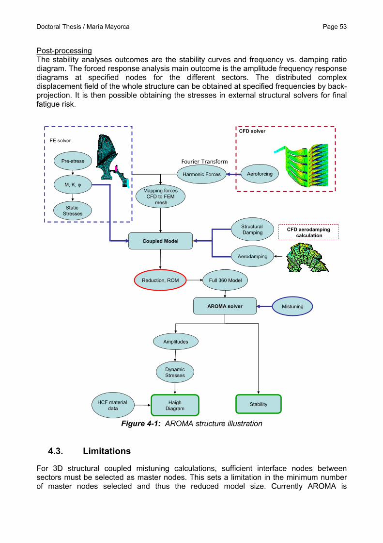
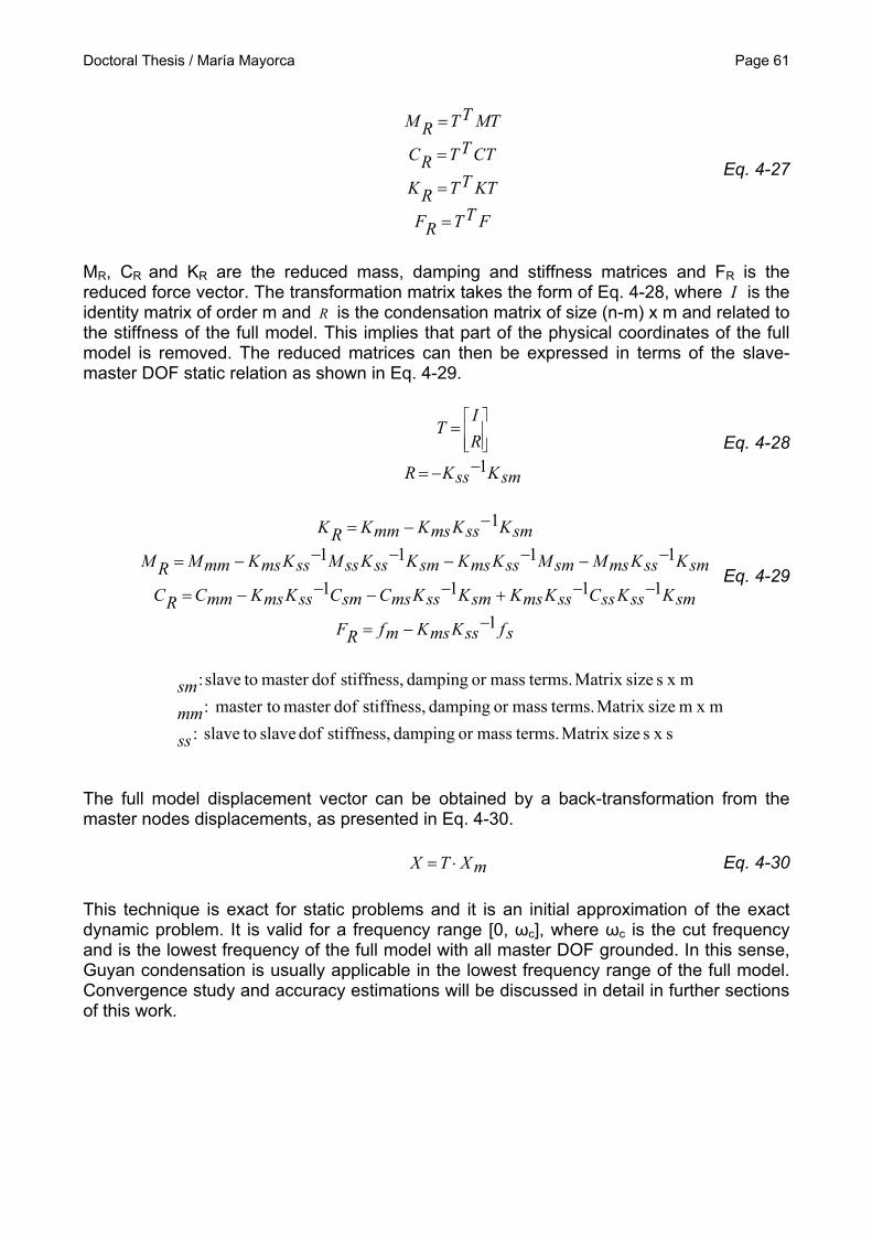
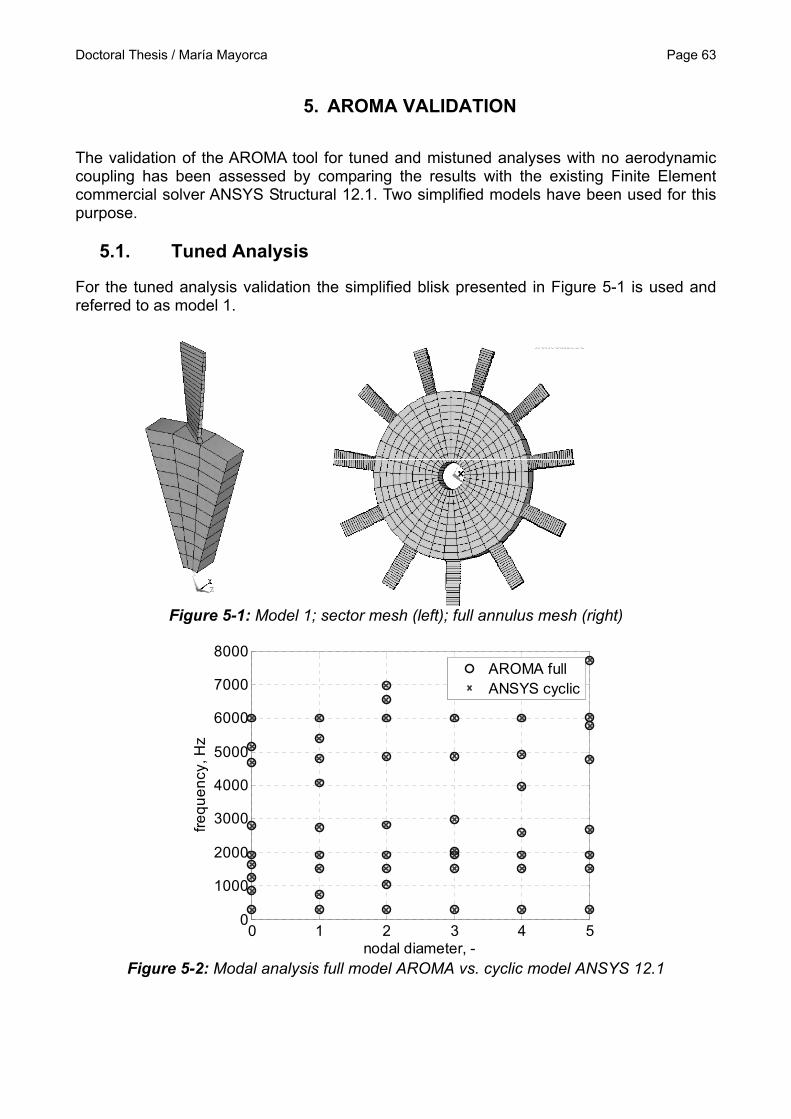
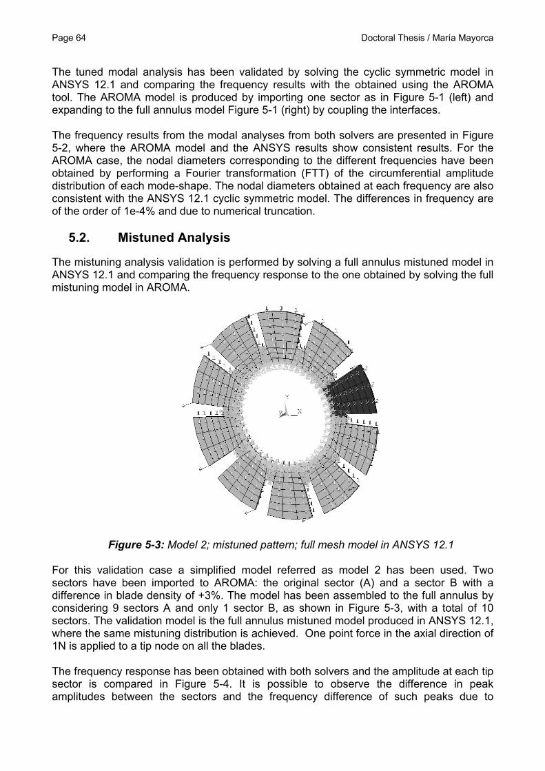
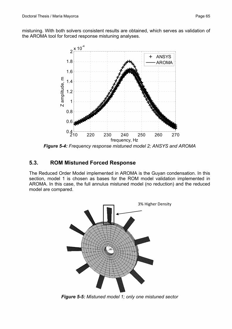
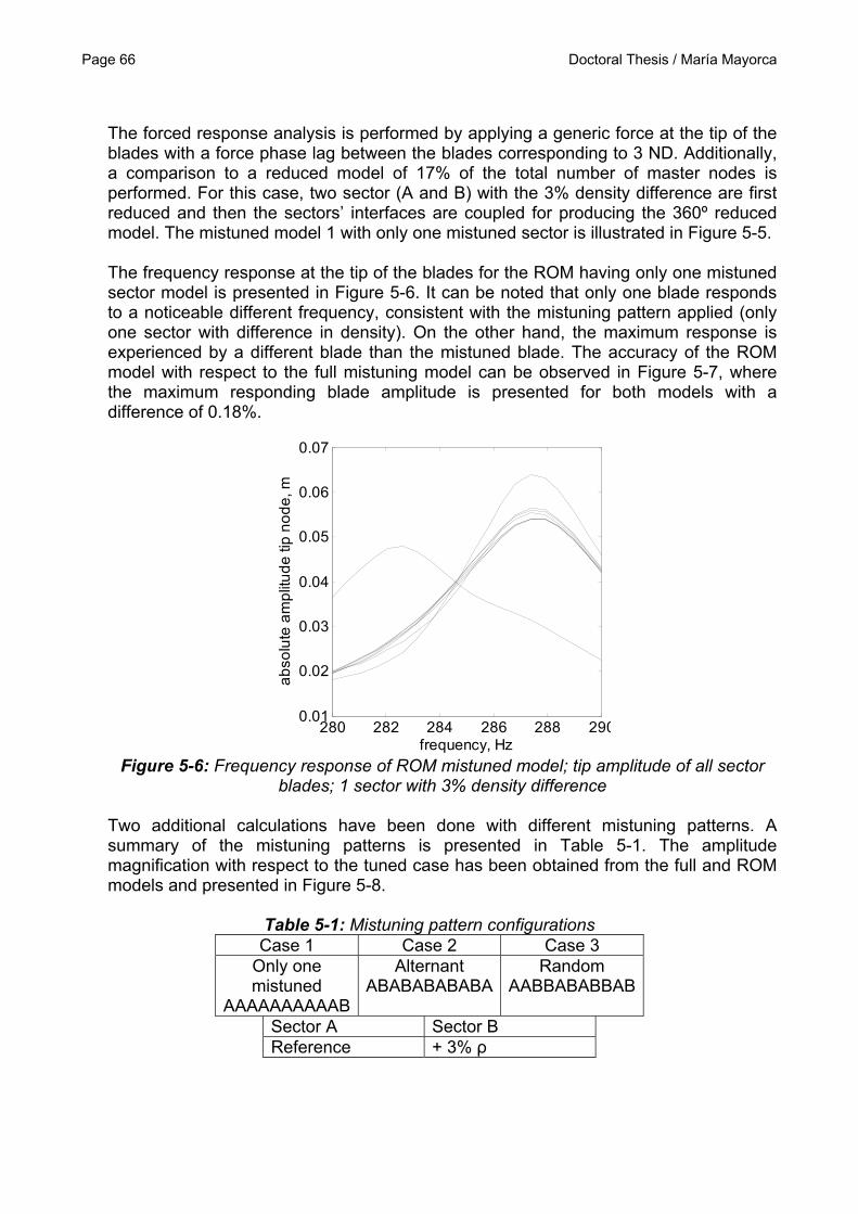
analyses, adapted from Seinturier (2008) ................................................................... 39 Figure 4-1: AROMA structure illustration .......................................................................... 53 Figure 5-1: Model 1; sector mesh (left); full annulus mesh (right) ...................................... 63 Figure 5-2: Modal analysis full model AROMA vs. cyclic model ANSYS 12.1 ................... 63 Figure 5-3: Model 2; Mistuned pattern; full mesh model in ANSYS 12.1 ........................... 64 Figure 5-4: Frequency response mistuned model 2; ANSYS and AROMA ........................ 65 Figure 5-5: Mistuned model 1; only one mistuned sector .................................................. 65 Figure 5-6: Frequency response of ROM mistuned model; tip amplitude of all sector

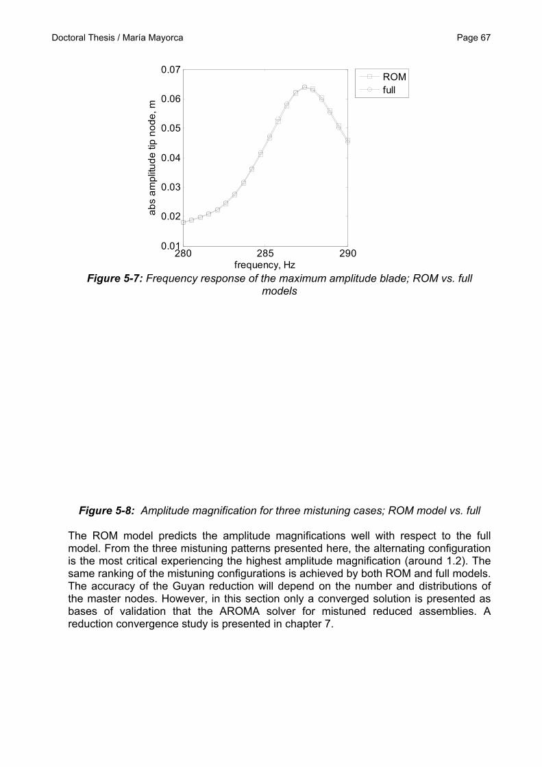
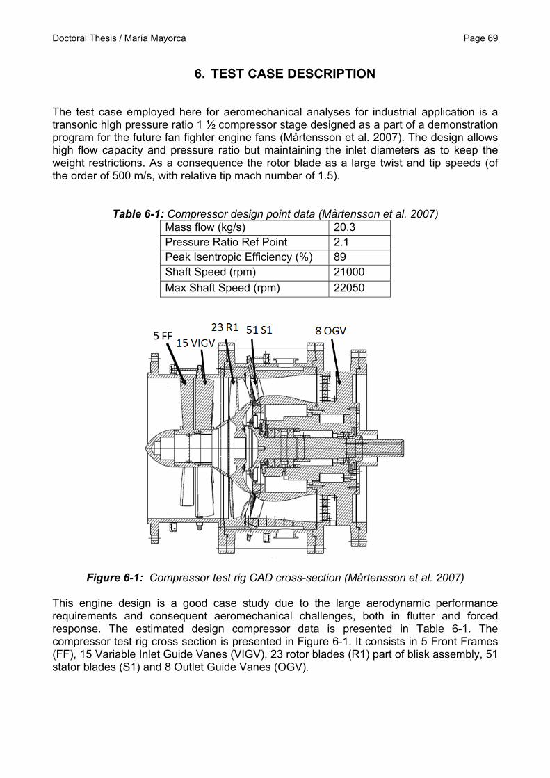
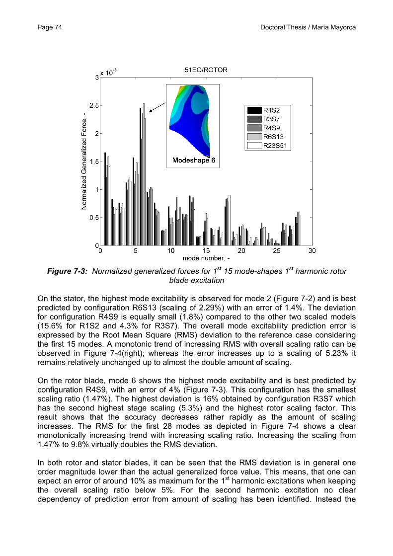
blades; 1 sector with 3% density difference ................................................................ 66 Figure 5-7: Frequency response of the maximum amplitude blade; ROM vs. full models . 67 Figure 5-8: Amplitude magnification for three mistuning cases; ROM model vs. full ........ 67 Figure 6-1: Compressor test rig CAD cross-section (Mårtensson et al. 2007) .................. 69 Figure 7-1: 3D scaled mesh at maximum span; R3S7 ...................................................... 72 Figure 7-2: Normalized generalized forces for 1st 15 mode-shapes 1st harmonic stator

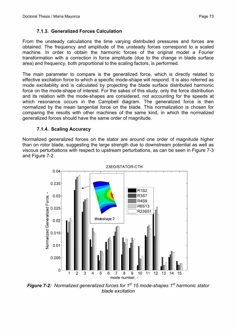
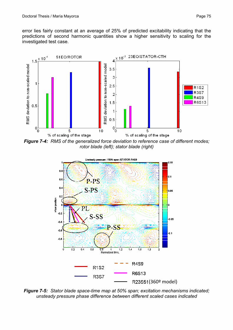
blade excitation ........................................................................................................... 73 Figure 7-3: Normalized generalized forces for 1st 15 mode-shapes 1st harmonic rotor

blade excitation ........................................................................................................... 74 Figure 7-4: RMS of the generalized force deviation to reference case of different modes;

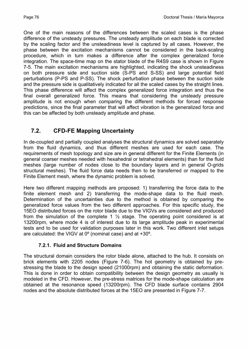
rotor blade (left); stator blade (right) ........................................................................... 75 Figure 7-5: Stator blade space-time map at 50% span; excitation mechanisms indicated;

unsteady pressure phase difference between different scaled cases indicated ......... 75


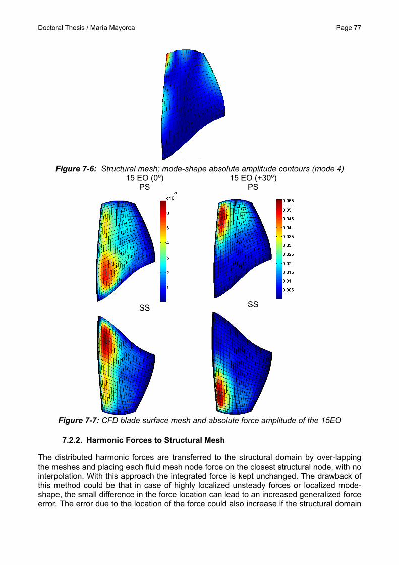
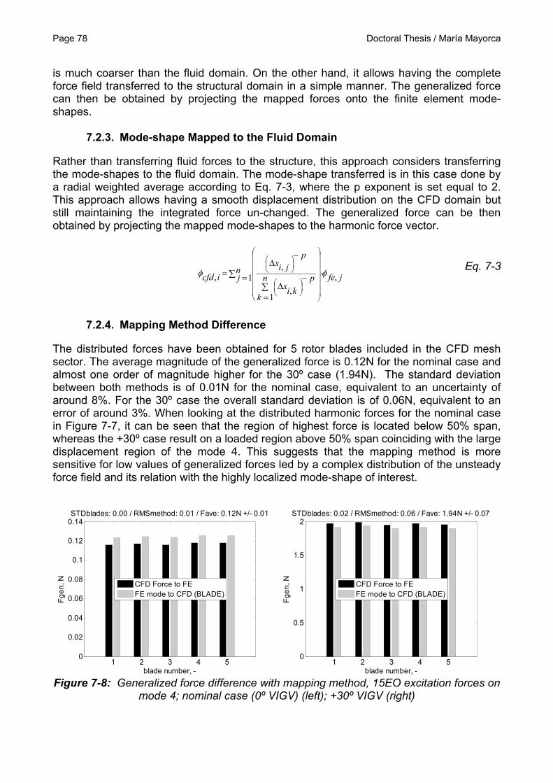
Figure 7-6: Structural mesh; mode-shape absolute amplitude contours (mode 4) ............ 77 Figure 7-7: CFD blade surface mesh and absolute force amplitude of the 15EO .............. 77 Figure 7-8: Generalized force difference with mapping method, 15EO excitation forces on

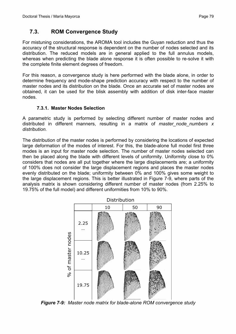
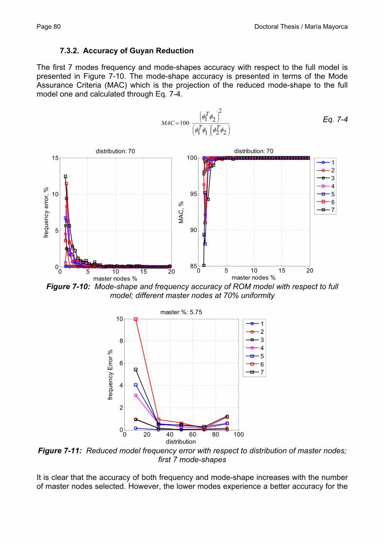
mode 4; nominal case (0º VIGV) (above); +30º VIGV (below) .................................... 78 Figure 7-9: Master node matrix for blade-alone ROM convergence study ........................ 79 Figure 7-10: Mode-shape and frequency accuracy of ROM model with respect to full

model; different master nodes at 70% uniformity ........................................................ 80 Figure 7-11: Reduced model frequency error with respect to distribution of master nodes;

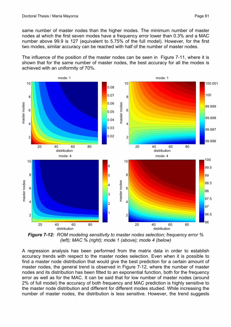
first 7 mode-shapes .................................................................................................... 80 Figure 7-12: ROM modeling sensitivity to master nodes selection; frequency error % (left);

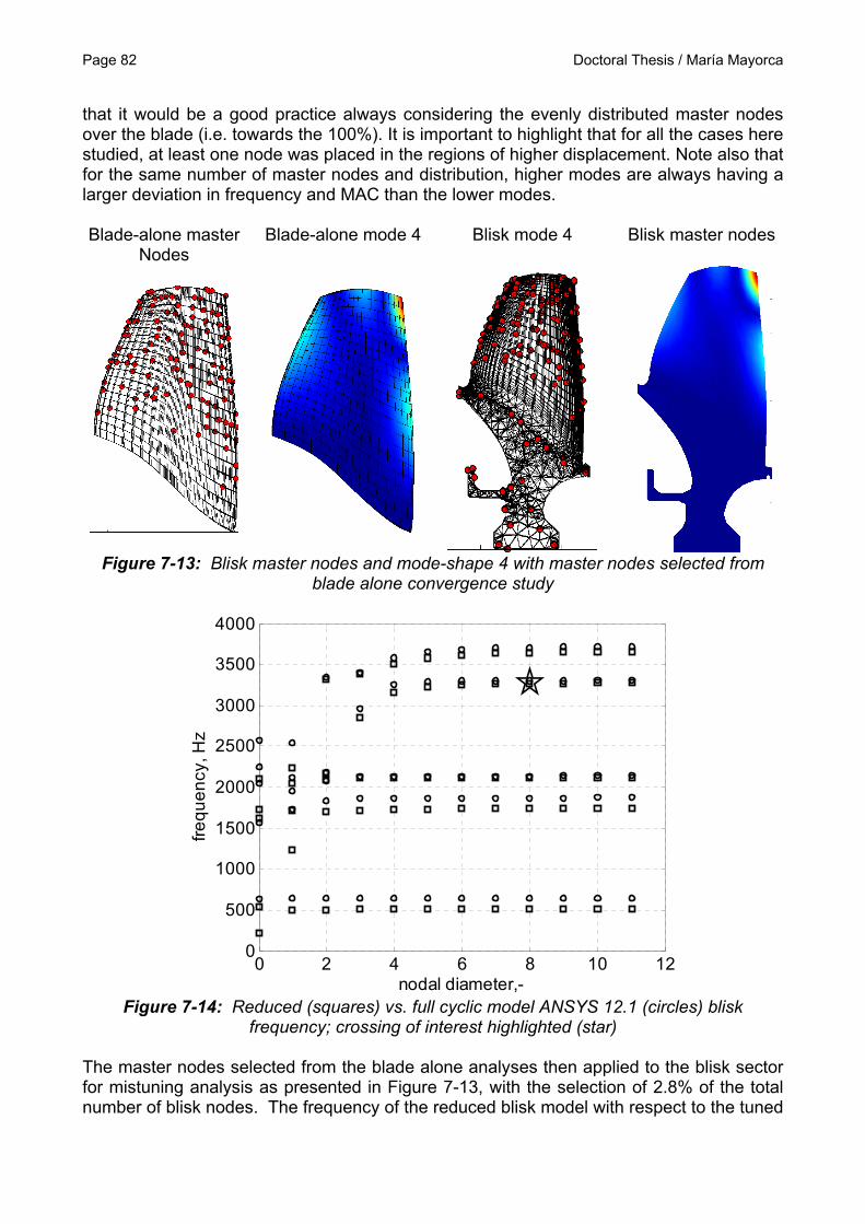
MAC % (right); mode 1 (above); mode 4 (below) ....................................................... 81 Figure 7-13: Blisk master nodes and mode-shape 4 with master nodes selected from

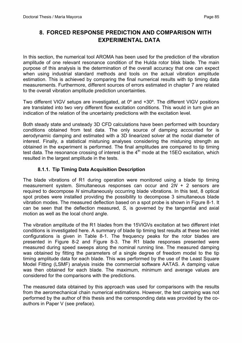
blade alone convergence study .................................................................................. 82 Figure 7-14: Reduced (squares) vs. full cyclic model ANSYS 12.1 (circles) blisk

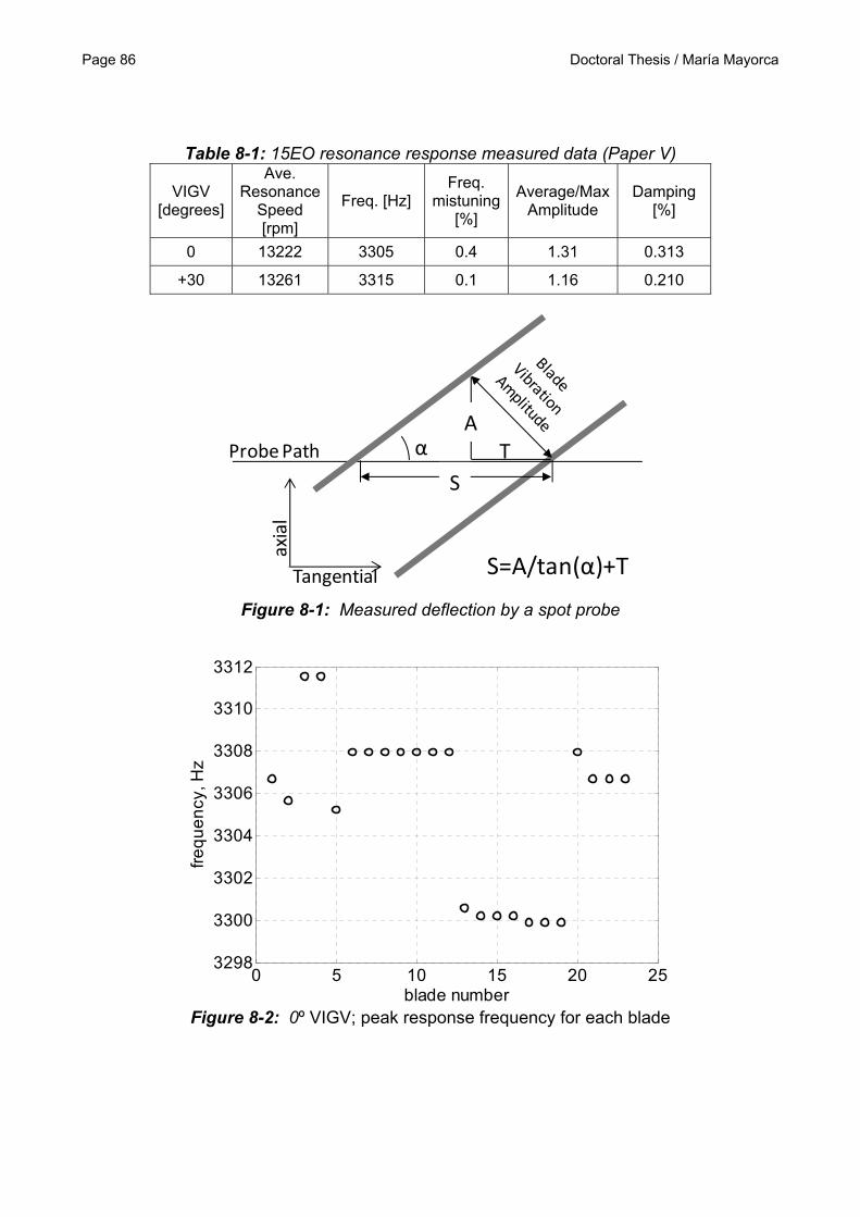
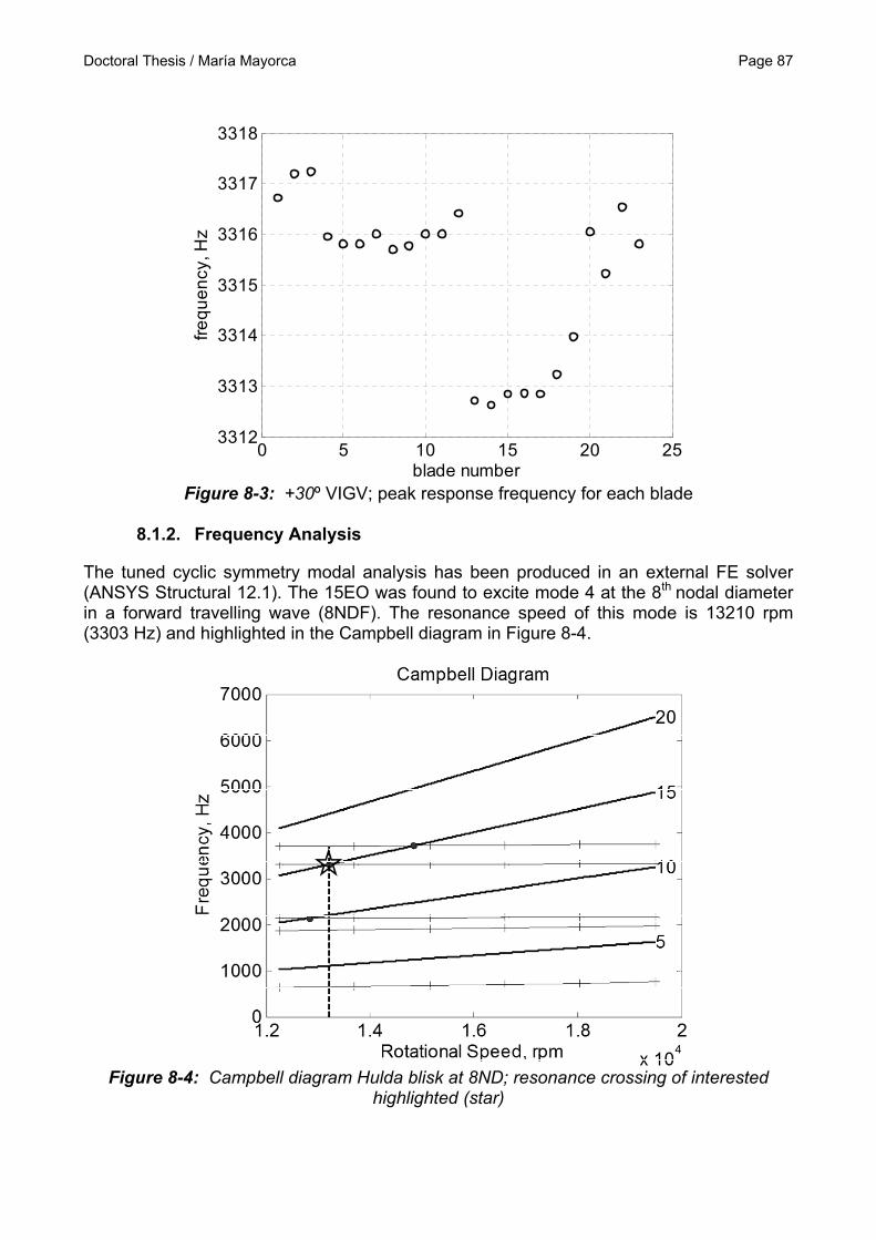
frequency; crossing of interest highlighted (star) ........................................................ 82 Figure 8-1: Measured deflection by a spot probe .............................................................. 86 Figure 8-2: 0º VIGV; peak response frequency for each blade ......................................... 86 Figure 8-3: +30º VIGV; peak response frequency for each blade ..................................... 87 Figure 8-4: Campbell diagram Hulda blisk at 8ND; resonance crossing of interested

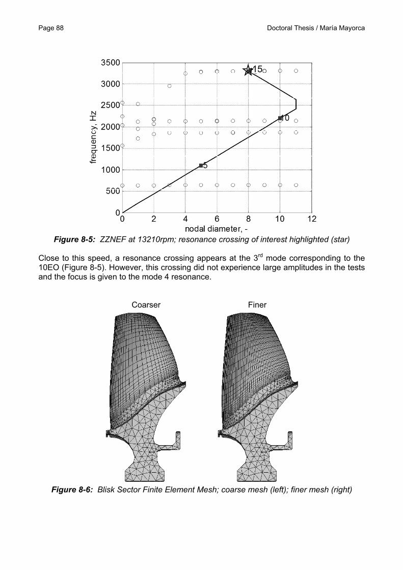
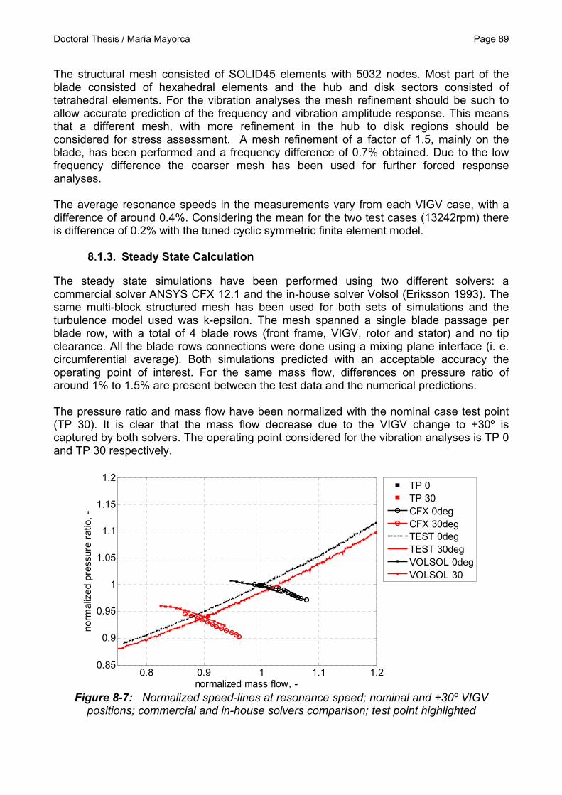
highlighted (star) ......................................................................................................... 87 Figure 8-5: ZZNEF at 13210rpm; resonance crossing of interest highlighted (star) .......... 88 Figure 8-6: Blisk Sector Finite Element Mesh; coarse mesh (left); finer mesh (right) ....... 88 Figure 8-7: Normalized speed-lines at resonance speed; nominal and +30º VIGV

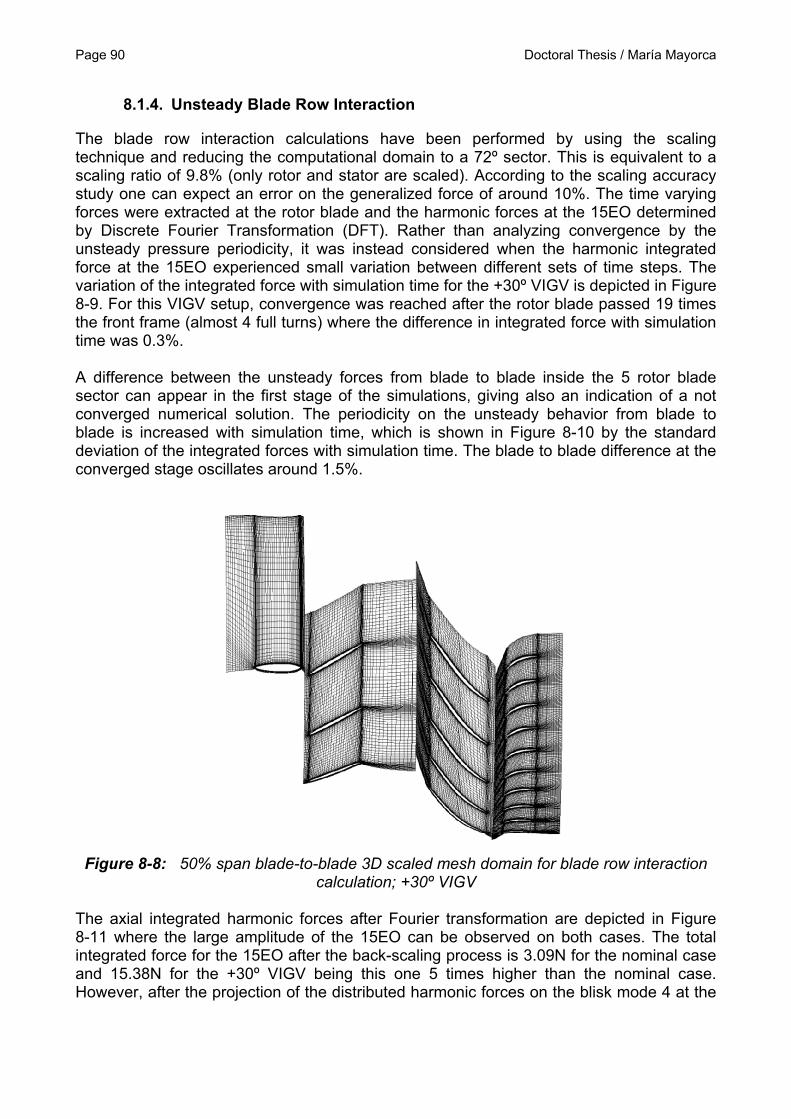
positions; commercial and in-house solvers comparison; Test point highlighted ........ 89 Figure 8-8: 50% span blade-to-blade 3D scaled mesh domain for blade row interaction

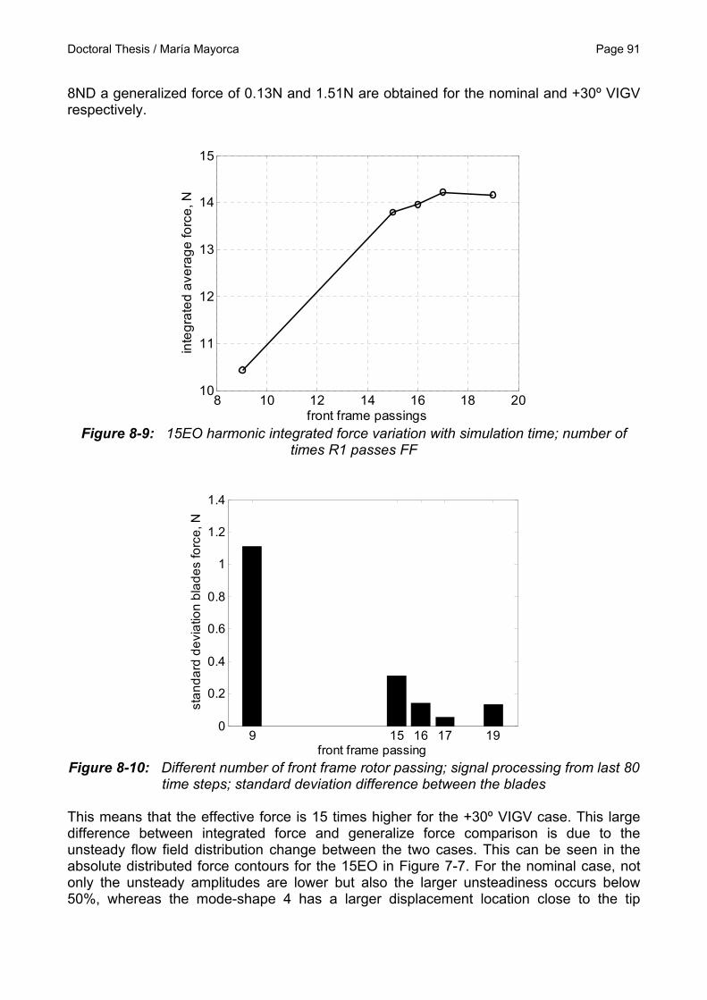
calculation; +30º VIGV ................................................................................................ 90 Figure 8-9: 15EO harmonic integrated force variation with simulation time; Number of

times R1 passes FF .................................................................................................... 91 Figure 8-10: Different number of front frame rotor passing; signal processing from last 80

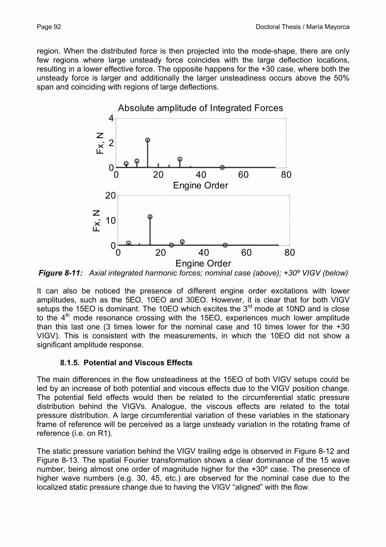
time steps; standard deviation difference between the blades ................................... 91 Figure 8-11: Axial integrated harmonic forces; nominal case (above); +30º VIGV (below)

................................................................................................................................... 92 Figure 8-12: 0 º VIGV; downstream VIGV trailing edge static pressure circumferential

variation; 90% span (above); wave number after spatial Fourier transformation (below) ................................................................................................................................... 93

Figure 8-13: +30 º VIGV; downstream VIGV trailing edge static pressure circumferential variation; 90% span (above); wave number after spatial Fourier transformation (below) ................................................................................................................................... 93

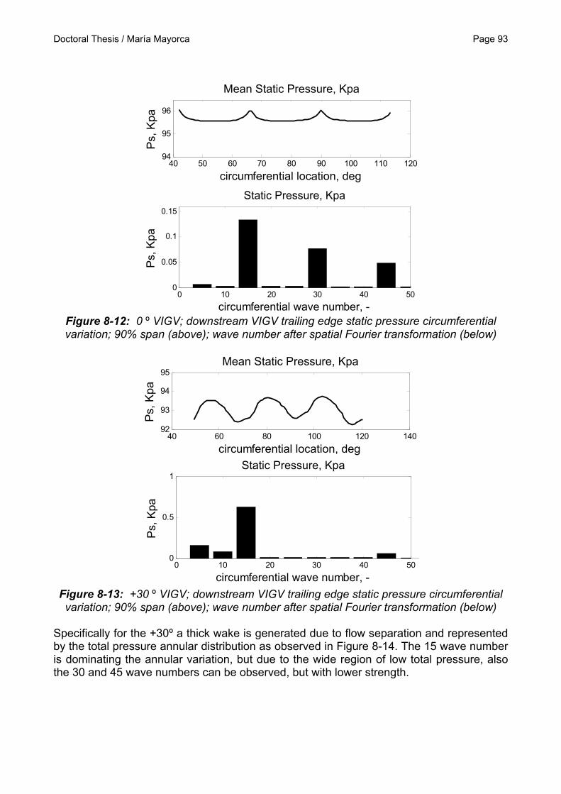
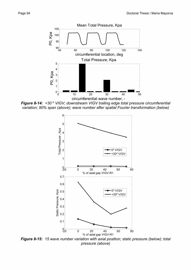
Figure 8-14: +30 º VIGV; downstream VIGV trailing edge total pressure circumferential variation; 90% span (above); wave number after spatial Fourier transformation (below) ................................................................................................................................... 94

Figure 8-15: 15 wave number variation with axial position; static pressure (below); total pressure (above)......................................................................................................... 94

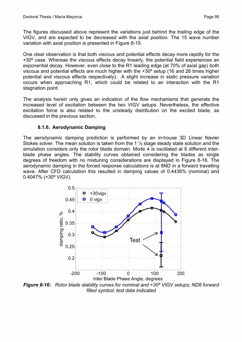
Figure 8-16: Rotor blade stability curves for nominal and +30º VIGV setups; ND8 forward filled symbol; test data indicated ................................................................................. 95

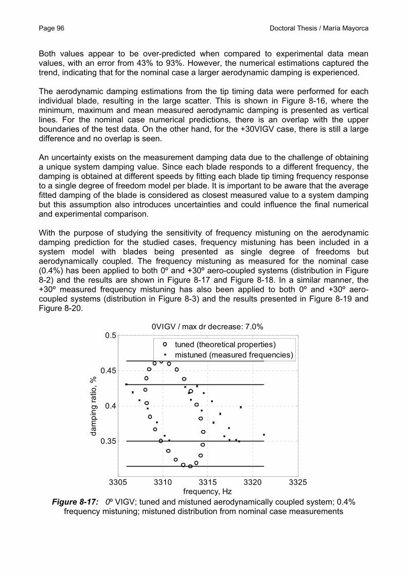
Figure 8-17: 0º VIGV; tuned and mistuned aerodynamically coupled system; 0.4% frequency mistuning; mistuned distribution from nominal case measurements .......... 96

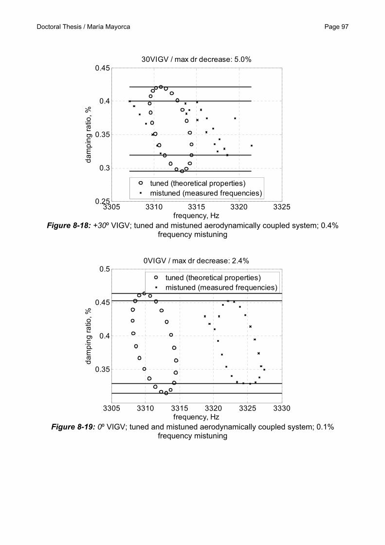
Figure 8-18: +30º VIGV; tuned and mistuned aerodynamically coupled system; 0.4% frequency mistuning .................................................................................................... 97


Figure 8-19: 0º VIGV; tuned and mistuned aerodynamically coupled system; 0.1% frequency mistuning .................................................................................................... 97

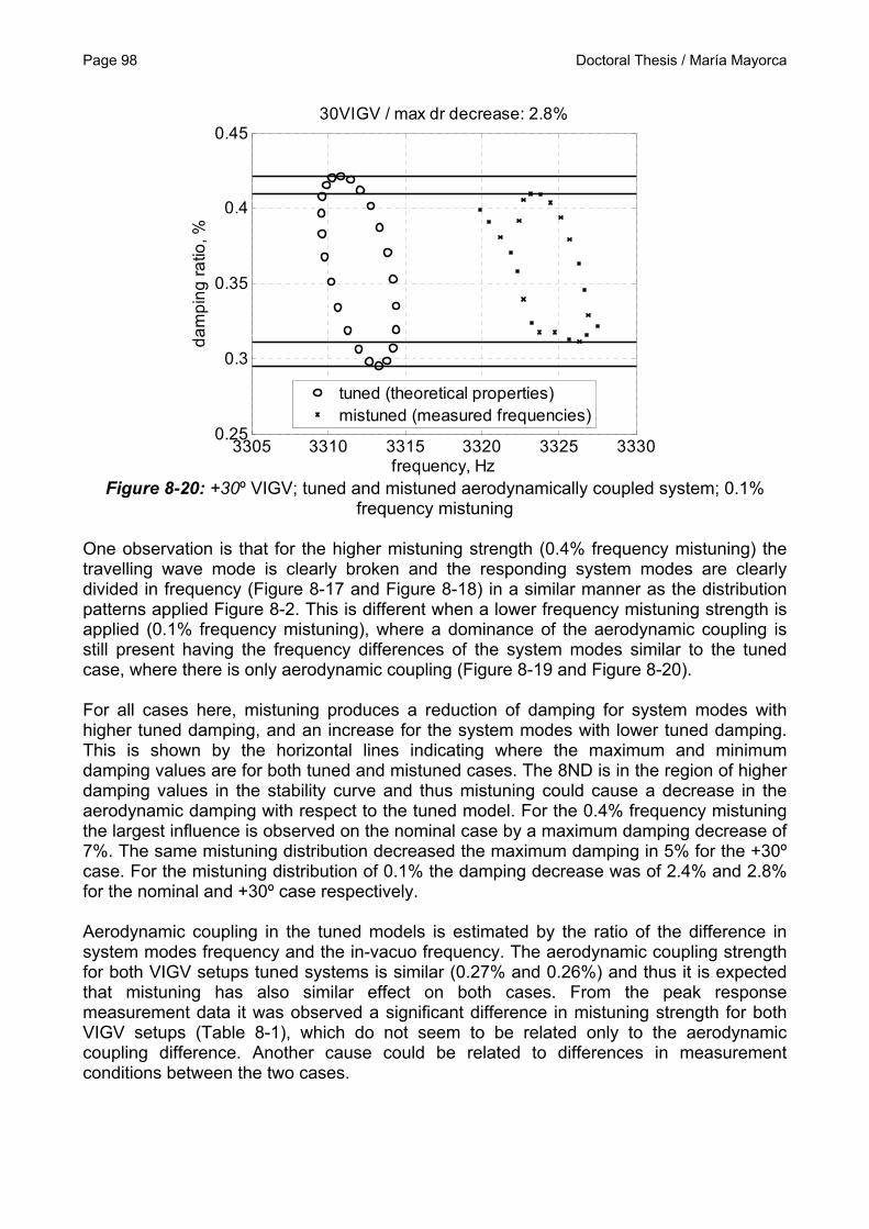
Figure 8-20: +30º VIGV; tuned and mistuned aerodynamically coupled system; 0.1% frequency mistuning .................................................................................................... 98

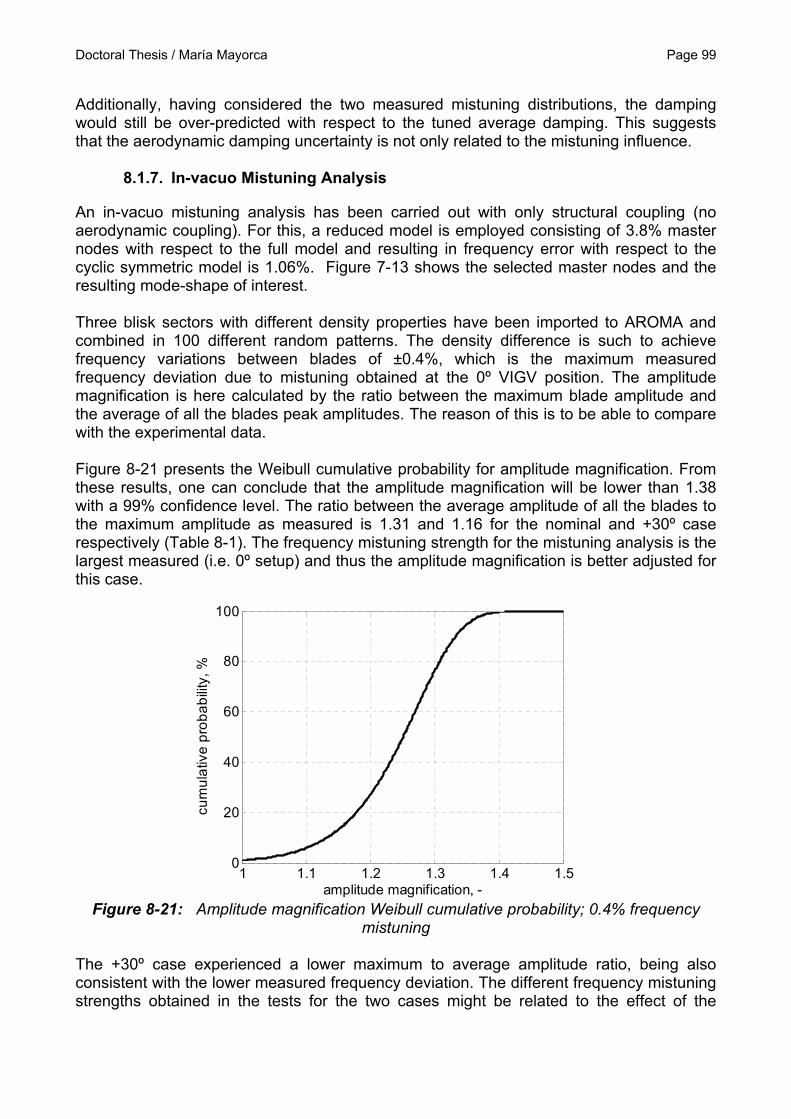
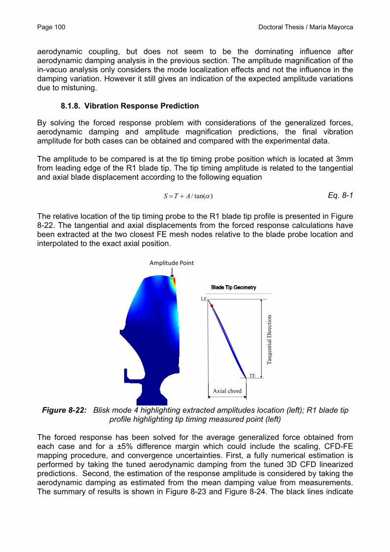
Figure 8-21: Amplitude magnification Weibull cumulative probability; 0.4% frequency mistuning .................................................................................................................... 99

Figure 8-22: Blisk mode 4 highlighting extracted amplitudes location (left); R1 blade tip profile highlighting tip timing measured point (left) .................................................... 100

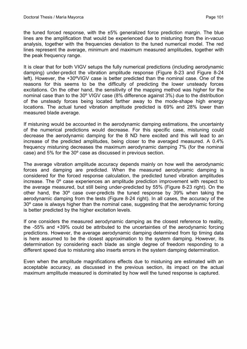
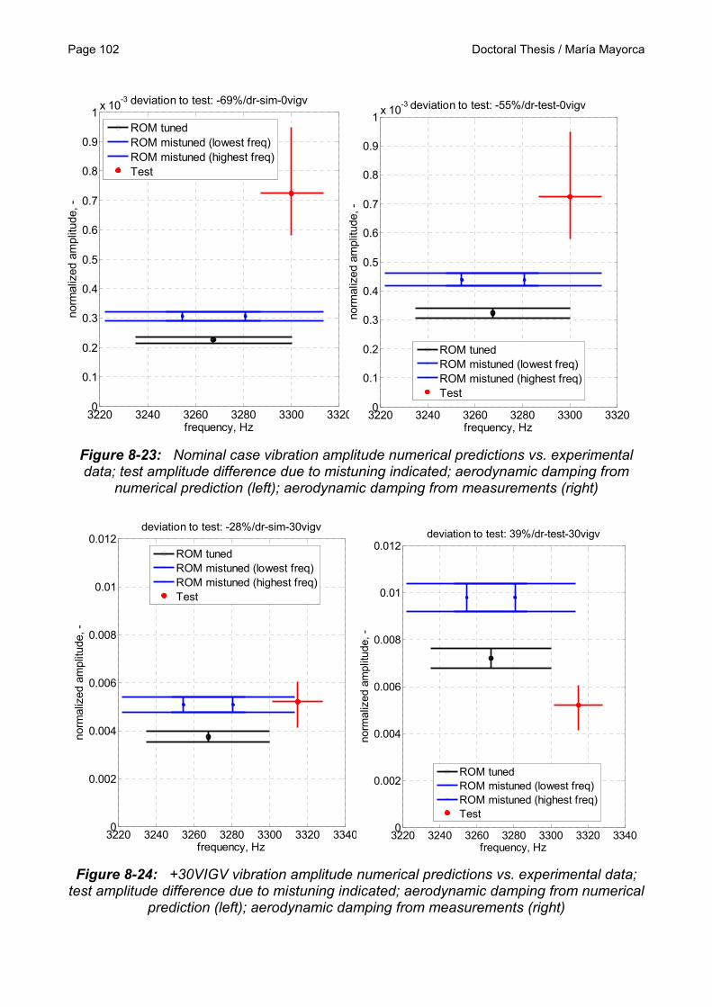
Figure 8-23: Nominal case vibration amplitude numerical predictions vs. experimental data; test amplitude difference due to mistuning indicated; aerodynamic damping from numerical prediction (left); aerodynamic damping from measurements (right) ......... 102

Figure 8-24: +30VIGV vibration amplitude numerical predictions vs. experimental data; test amplitude difference due to mistuning indicated; aerodynamic damping from numerical prediction (left); aerodynamic damping from measurements (right) ......... 102

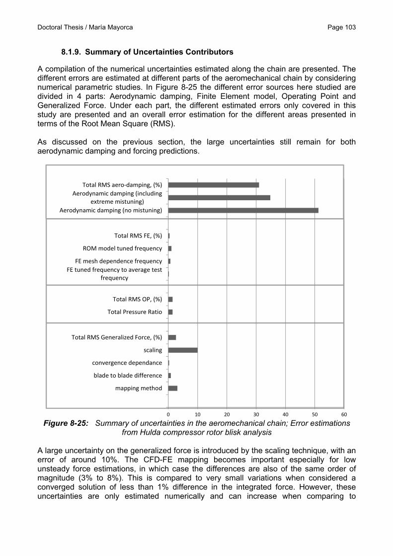
Figure 8-25: Summary of uncertainties in the aeromechanical chain; Error estimations from Hulda compressor rotor blisk analysis .............................................................. 103

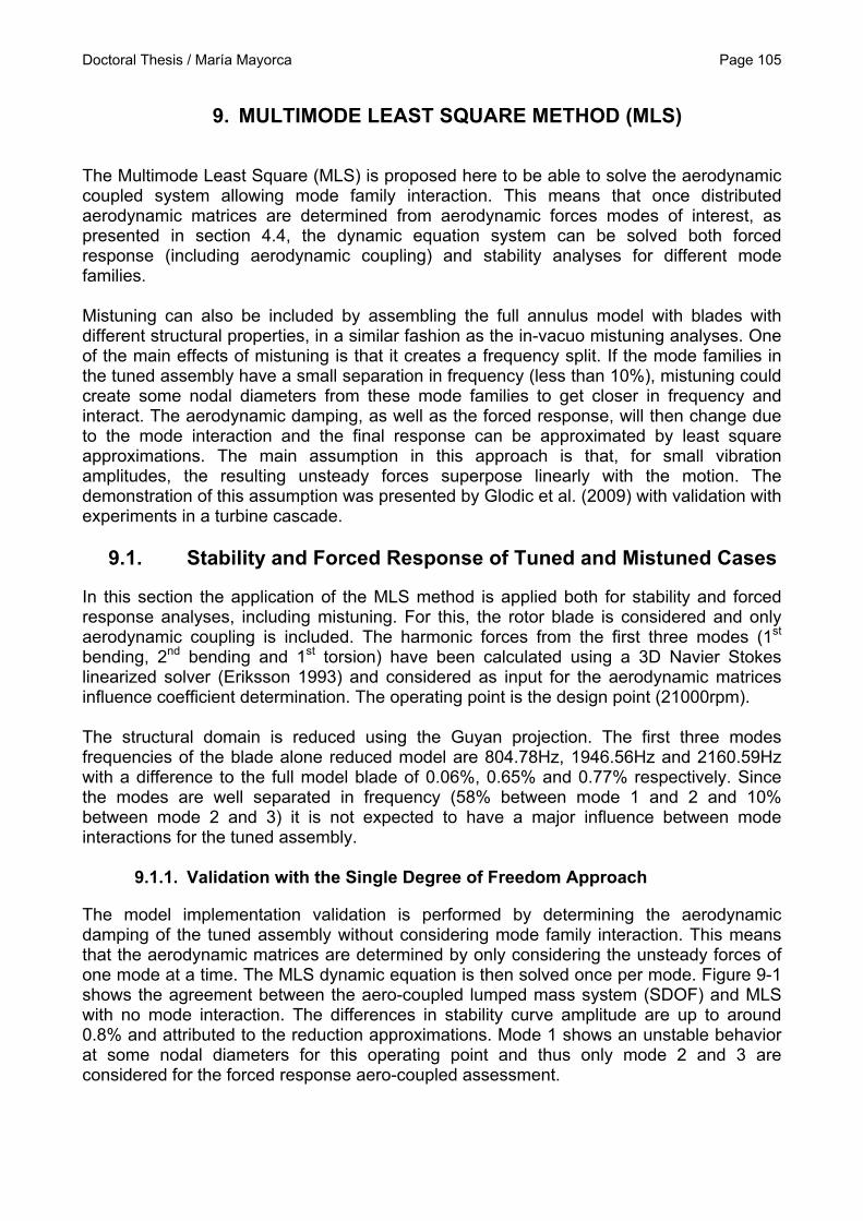
Figure 9-1: Tuned stability comparison between lumped mass system (SDOF) and the reduced MLS ............................................................................................................ 106

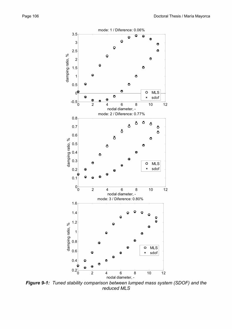
Figure 9-2: Vibration amplitude for different nodal diameters considering aerodynamic damping; mode 2 (above); mode 3 (below); different methods ................................. 107

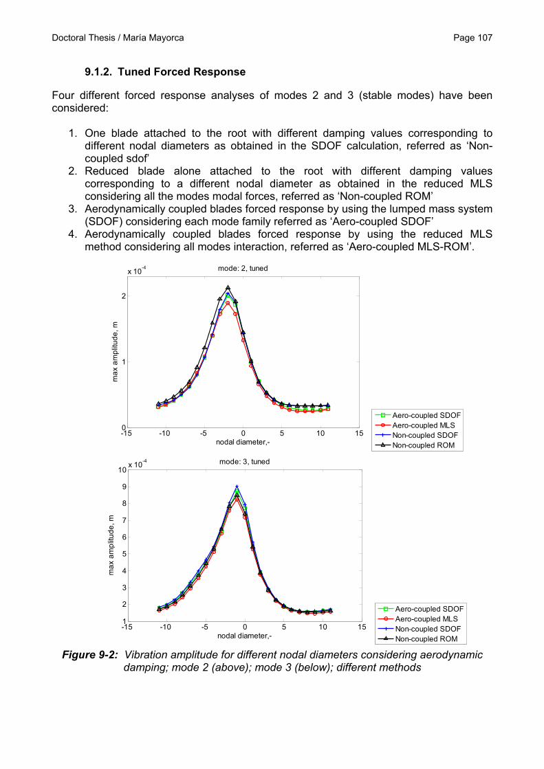
Figure 9-3: Amplitude magnification due to mistuning considering aerodynamic coupling; MLS; mode 2 (above); mode 3 (below) ..................................................................... 108

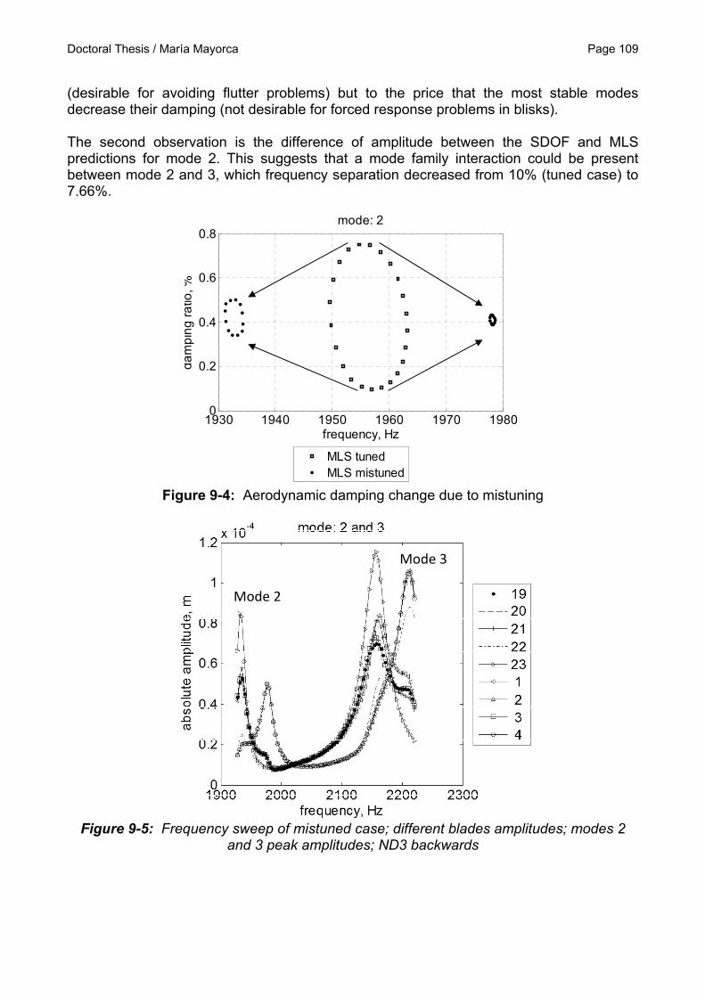
Figure 9-4: Aerodynamic damping change due to mistuning .......................................... 109 Figure 9-5: Frequency sweep of mistuned case; different blades amplitudes; modes 2 and

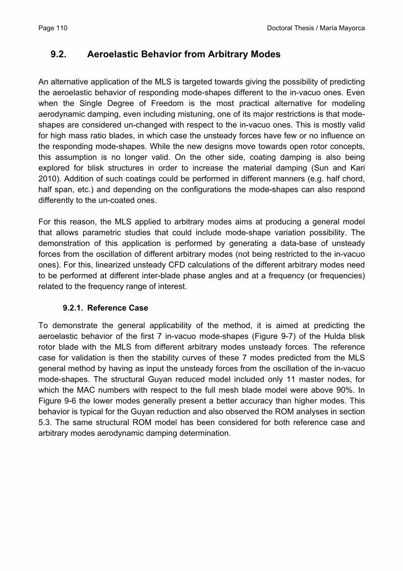
3 peak amplitudes; ND3 backwards ......................................................................... 109 Figure 9-6: Different sets of master nodes selected (above); full to reduced model MAC

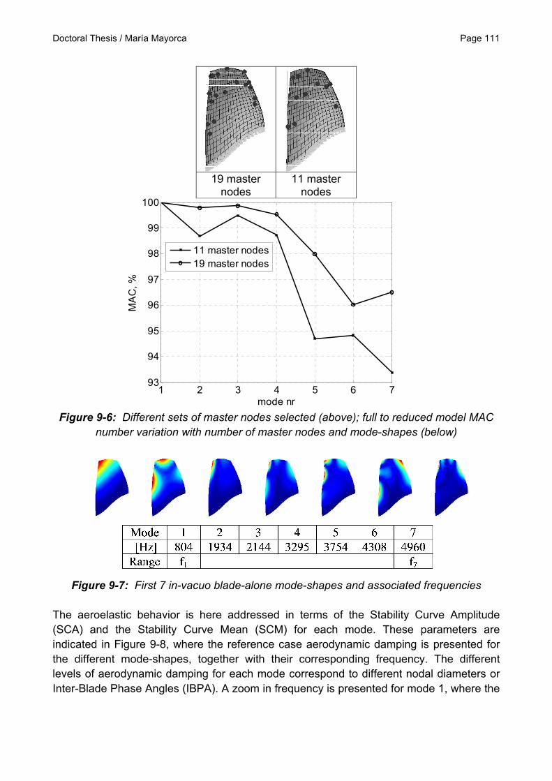
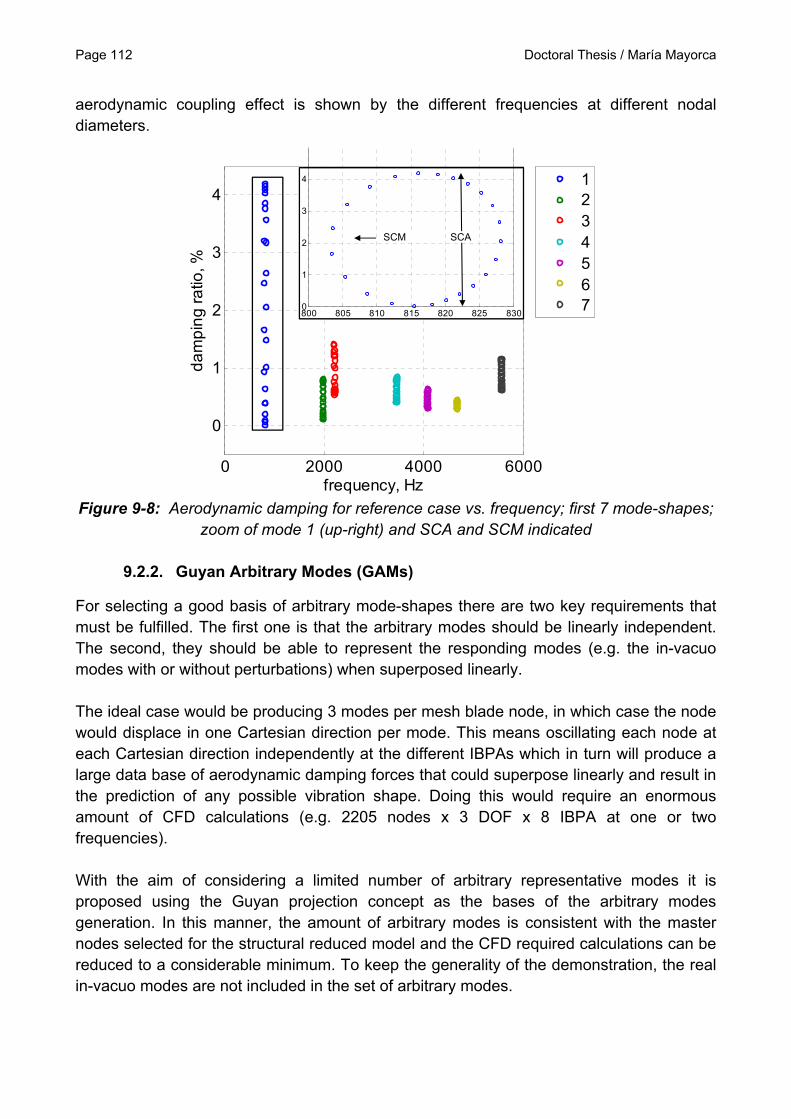
number variation with number of master nodes and mode-shapes (below) .............. 111 Figure 9-7: First 7 in-vacuo blade-alone mode-shapes and associated frequencies ...... 111 Figure 9-8: Aerodynamic damping for reference case vs. frequency; first 7 mode-shapes;

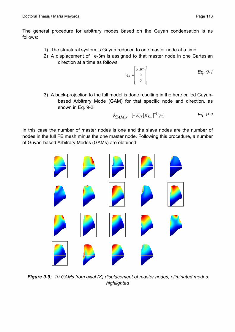
zoom of mode 1 (up-right) and SCA and SCM indicated .......................................... 112 Figure 9-9: 19 GAMs from axial (X) displacement of master nodes; eliminated modes

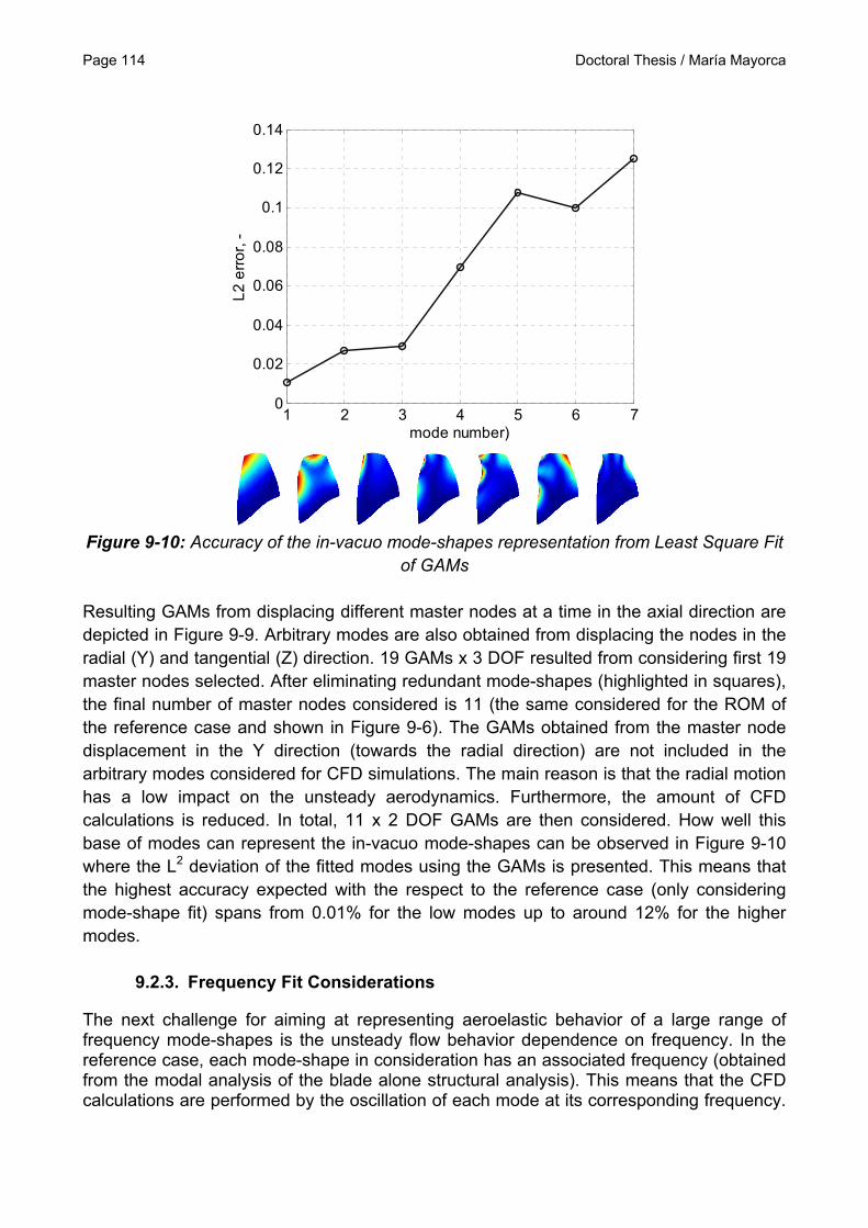
highlighted ................................................................................................................ 113 Figure 9-10: Accuracy of the in-vacuo mode-shapes representation from Least Square Fit

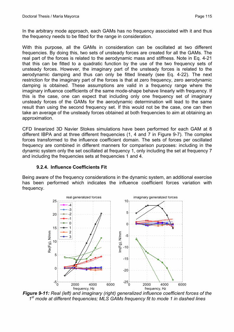
of GAMs .................................................................................................................... 114 Figure 9-11: Real (left) and imaginary (right) generalized influence coefficient forces of the

1st mode at different frequencies; MLS GAMs frequency fit to mode 1 in dashed lines ................................................................................................................................. 115

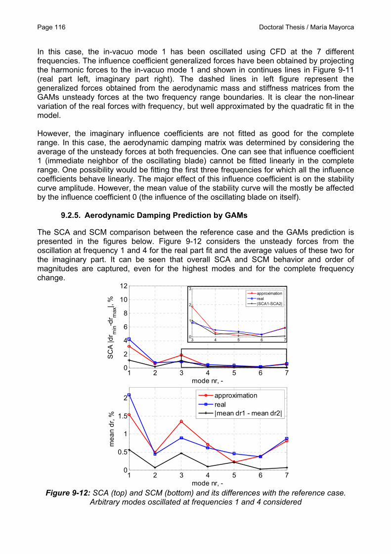
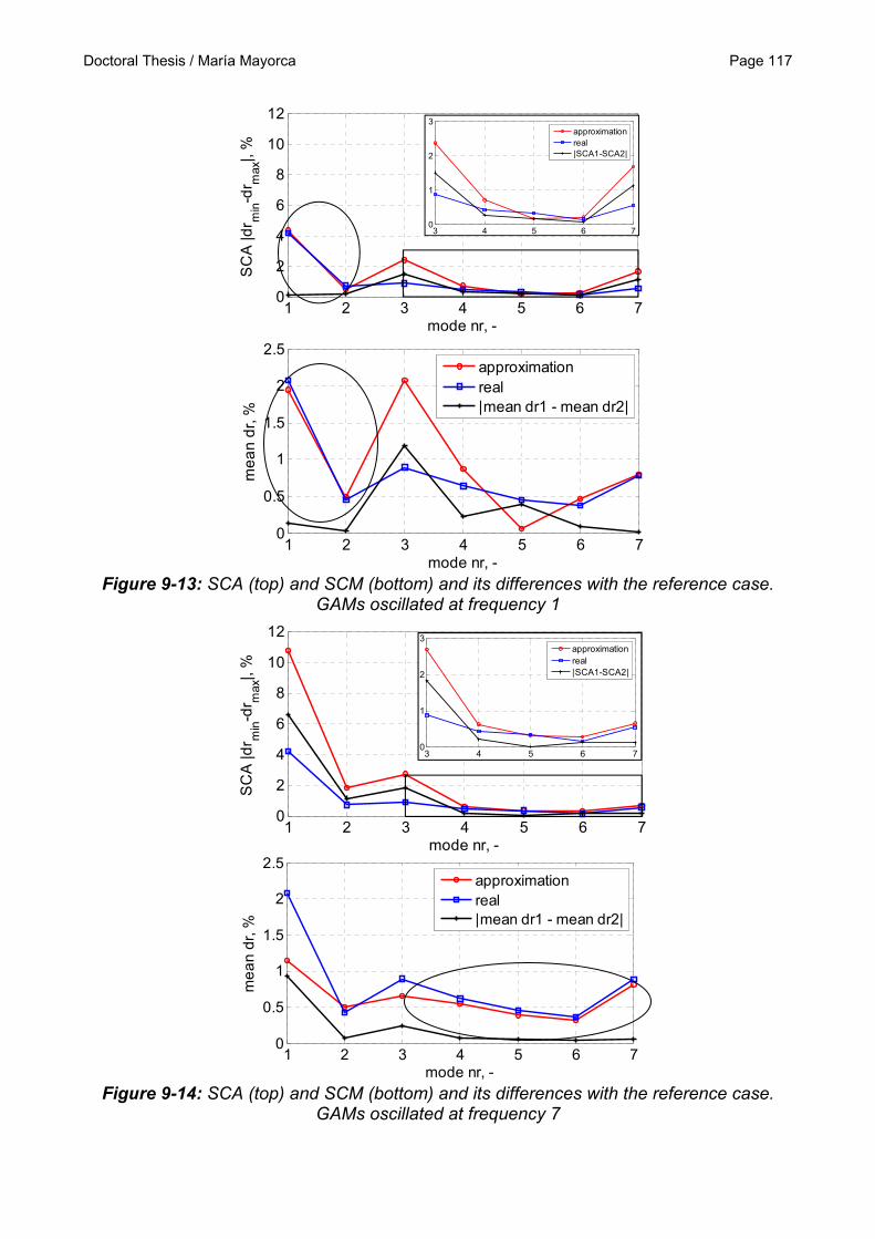
Figure 9-12: SCA (top) and SCM (bottom) and its differences with the reference case. Arbitrary modes oscillated at frequencies 1 and 4 considered .................................. 116

Figure 9-13: SCA (top) and SCM (bottom) and its differences with the reference case. GAMs oscillated at frequency 1 ................................................................................ 117

Figure 9-14: SCA (top) and SCM (bottom) and its differences with the reference case. GAMs oscillated at frequency 7 ................................................................................ 117

LIST OF TABLES

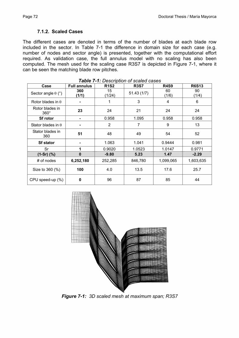
Table 5-1: mistuning pattern configurations ....................................................................... 66 Table 6-1: Compressor Design Point Data (Mårtensson et al. 2007) ................................. 69 Table 7-1: Description of scaled cases .............................................................................. 72 Table 8-1: 15EO resonance response measured data (Paper V) ...................................... 86


NOMENCLATURE

Latin Symbols

A circulant aerodynamic matrix, maximum oscillation amplitude [m], axial vibration motion at test point location [m]

Amp maximum absolute oscillation amplitude [m]

a generalized coordinates [-] b maximum mass normalized eigen-vector [m] C damping matrix [Ns/m] c blade chord [m], linear damping [Ns/m] E Verdon stability parameter, related to edge wise bending mode-shape F force [N], related to flexion or bending mode-shape f frequency [Hz]

G matrix with modal force vectors [N] g generalized force [N]

H matrix with modal force vectors divided by the frequency I identity matrix [-]

i complex number 1 , counter of mode number in MLS method derivation [-]

Im refers to the imaginary part of a complex number K stiffness matrix [N/m] k reduced frequency [-], modal stiffness [N/m], counter of node number

in the MLS method derivation [-] 2L least square

M mass matrix [kg] m modal mass [kg], total number of modes considered in the MLS [-] N number of blades P matrix with modal displacement vectors [m] Re refers to the real part of a complex number Sf scaling factor [-]

Sr scaling ratio [-] T oscillation period [1/s], tangential vibration motion [m] ,reduction

transformation matrix, related to torsion mode-shape t time [s] U mode kinetic energy [J] u flow speed [m/s] Q amplitude factor [-], displacement in generalized coordinates [N]

cycleW work per oscillation cycle [J]

X physical coordinates displacement vector [m] y approximated solution by mode superposition [m]


Greek Symbols

local chord angle, [rad]

critical damping ratio [-]

eigen vector [-]

logarithmic decrement [-] eigen-value [-] stress [Pa], inter-blade phase angle [rad] loss factor [-]

speed [rpm] frequency [rad/s] Subscripts

AERO denoting system aerodynamic matrices aero denoting influence coefficient aerodynamic matrices crit related to the critical damping cycle per oscillation cycle

ex excitation f fatigue

ic influence coefficient domain m maximum, master degree of freedom n related to the natural frequency p empirical high static stress in alternating stress limit

R related to reduced matrixes s slave degree of freedoms STRU denoting structural system matrices u ultimate y yield

yc cyclic yield

twm travelling wave mode domain Superscripts

k node number counter m blade influence counter, mode counter n blade influence counter T transpose

inter-blade phase angle ^ denoting a complex variable


Abbreviations

AM Arbitrary Mode-shapes AMM Asymptotic Mistuning Model AROMA Aeroelastic Reduced Order Modeling Analyses CFD Computational Fluid Dynamics CMS Component Mode Synthesis DFT Discrete Fourier Transformation DOF Degree Of Freedom(s) EO Engine Order FE Finite Element GAM Guyan Arbitrary Mode HCF High Cycle Fatigue IBPA Inter-Blade Phase Angle FF Front Frame FMM Fundamental Mistuning Model FOD Foreign Object Damage HPC High Pressure Compressor IP Intermediate Pressure LPC Low Pressure Compressor LPT Low Pressure Turbine MAC Mode Assurance Criteria MD Modal Decomposition MLS Multimode Least Square ND, nd Nodal Diameter NSV Non-Synchronous Vibration OPR Overall Pressure Ratio PS Pressure Side RMS Root Mean Square SCA Stability Curve Amplitude SCM Stability Curve Mean SS Suction Side SV Synchronous Vibration S1 Stator 1 OGV Outlet Guide Vanes OP Operating Point PL Phase Line ROM Reduced Order Modeling R1 Rotor 1 SDOF Single Degree of Freedom TWM Travelling Wave Mode VIGV Variable Inlet Guide Vane ZZENF Zig-zag Engine-Order Nodal-Diameter Frequency 3D Three Dimensional Definitions

Blisk integrally bladed disk


Hot geometry blade geometry on operation as designed aerodynamically. Pre-stressed geometry

Campbell diagram frequency vs. frequency diagram where eigen frequencies are plotted against engine order excitation lines. Used for determination of resonance crossings.

Haigh diagram Alternant vs. mean stress diagram where high cycle fatigue material limits are presented. Used for determination of stress limits.


1. BACKGROUND

1.1. Gas Turbines

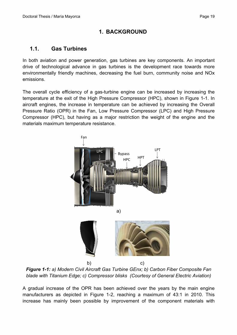
In both aviation and power generation, gas turbines are key components. An important drive of technological advance in gas turbines is the development race towards more environmentally friendly machines, decreasing the fuel burn, community noise and NOx emissions. The overall cycle efficiency of a gas-turbine engine can be increased by increasing the temperature at the exit of the High Pressure Compressor (HPC), shown in Figure 1-1. In aircraft engines, the increase in temperature can be achieved by increasing the Overall Pressure Ratio (OPR) in the Fan, Low Pressure Compressor (LPC) and High Pressure Compressor (HPC), but having as a major restriction the weight of the engine and the materials maximum temperature resistance.

Fan

LPC

HPC

LPT

HPTBypass

a)

b) c) Figure 1-1: a) Modern Civil Aircraft Gas Turbine GEnx; b) Carbon Fiber Composite Fan blade with Titanium Edge; c) Compressor blisks (Courtesy of General Electric Aviation)

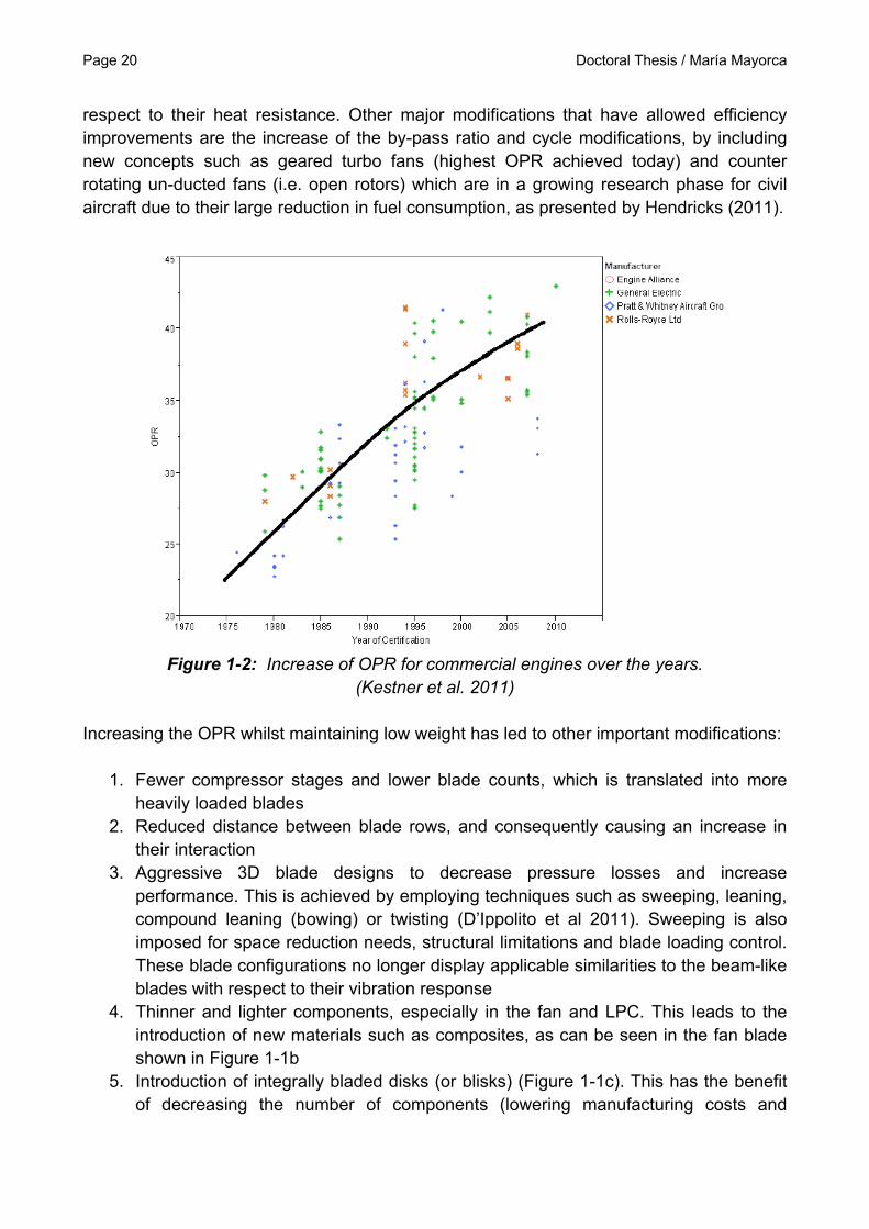
A gradual increase of the OPR has been achieved over the years by the main engine manufacturers as depicted in Figure 1-2, reaching a maximum of 43:1 in 2010. This increase has mainly been possible by improvement of the component materials with


respect to their heat resistance. Other major modifications that have allowed efficiency improvements are the increase of the by-pass ratio and cycle modifications, by including new concepts such as geared turbo fans (highest OPR achieved today) and counter rotating un-ducted fans (i.e. open rotors) which are in a growing research phase for civil aircraft due to their large reduction in fuel consumption, as presented by Hendricks (2011).

Figure 1-2: Increase of OPR for commercial engines over the years.

(Kestner et al. 2011) Increasing the OPR whilst maintaining low weight has led to other important modifications:

1. Fewer compressor stages and lower blade counts, which is translated into more heavily loaded blades

2. Reduced distance between blade rows, and consequently causing an increase in their interaction

3. Aggressive 3D blade designs to decrease pressure losses and increase performance. This is achieved by employing techniques such as sweeping, leaning, compound leaning (bowing) or twisting (D’Ippolito et al 2011). Sweeping is also imposed for space reduction needs, structural limitations and blade loading control. These blade configurations no longer display applicable similarities to the beam-like blades with respect to their vibration response

4. Thinner and lighter components, especially in the fan and LPC. This leads to the introduction of new materials such as composites, as can be seen in the fan blade shown in Figure 1-1b

5. Introduction of integrally bladed disks (or blisks) (Figure 1-1c). This has the benefit of decreasing the number of components (lowering manufacturing costs and


weight), increasing the effective hub to tip flow effective area and decreasing hub to blade connection leakage flows. On the other hand, there is no friction damping in the blade to disk connections, decreasing the possibilities for reducing blade vibration amplitudes

All these modifications result in increasing challenges concerning the structural integrity of the engine. Experience from old designs is thus not sufficient for new design, and instead advanced numerical tools, such as Computational Fluid Dynamics and Finite Element, are gradually being employed for aeromechanical predictions in an early design stage (Silkowski et al. 2001). This is of major importance in order to avoid having aeromechanical problems at the engine tests that could lead to major costs in re-design.

1.2. Aeromechanical Problems

Aeroemechanical problems in turbomachinery are mainly due to the interaction between the structures and the surrounding fluid flow. This interaction can lead to two main problems: High Cycle Fatigue (HCF) and flutter. High Cycle Fatigue problems are related to the structural components being exposed to a large number of cyclic fluid excitation forces and are often referred to as Forced Response problems. Depending on the excitation level, the component material might not withstand the required number of cycles in operation. This could lead to a failure of the blade at different levels, from a small blade tip material loss to a complete blade-off event.

Figure 1-3: Failed compressor blisk in the CT7-9B engine due to HCF (Australian

Transport Safety Bureau, 2010)

This was the case in the T55-L-11 around 1970, where long inter-locked turbine blades in the power turbine lost their friction damping due to rubbing, and a torsion mode in resonance produced the complete blade failure. After some time, the torsional force was enough to tear loose the complete power turbine and shaft (Leyes and Fleming, 1997). A more recent incident occurred in 2009, in a SAAB Co 340B aircraft where the left engine suffered damages resulting from the failure of four of the stage 1 compressor blisk blades


(Figure 1-3). After analysis of the causes “…the failures of the four blades on the subject blisk were the result of reverse-bending fatigue, under the influence of high frequency aerodynamic vibrations” (Australian Transport Safety Bureau, 2010). Instability or flutter problems are related to a self-excited situation, in which the interaction between the blade vibration and the flow establishes in such manner that the vibration amplitude increases rapidly and can result in an instant destruction of the complete engine. This work studies the last two problems (forced response and flutter) and thus are here exposed in more detail.

1.2.1. Forced Response

Forced response analyses are necessary in order to predict if the engine components, mainly the bladed disks, respond to vibration levels below the fatigue material margins.

tensilecompressive

safe

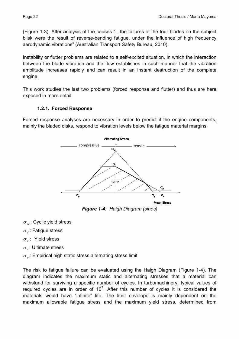
Figure 1-4: Haigh Diagram (sines)

yc : Cyclic yield stress

f : Fatigue stress

:y Yield stress

u : Ultimate stress

p : Empirical high static stress alternating stress limit

The risk to fatigue failure can be evaluated using the Haigh Diagram (Figure 1-4). The diagram indicates the maximum static and alternating stresses that a material can withstand for surviving a specific number of cycles. In turbomachinery, typical values of required cycles are in order of 107. After this number of cycles it is considered the materials would have “infinite” life. The limit envelope is mainly dependent on the maximum allowable fatigue stress and the maximum yield stress, determined from


material tests and application of statistical analyses. The most critical zone with respect to HCF is the right-hand side of the diagram, in which the component is exposed to tensile static stresses, favoring cracks initiation. Note that for a large level of static stresses, only a low level of alternating stresses is allowed before failure. This is the reason why when highly loaded blades are considered (e.g. fewer blades) the vibratory stress limit is reduced. Having defined the material limits it is then necessary to predict the static and alternating stresses at which the blades are exposed in the operating range of the engine. Static Stresses Static stresses are those appearing due to the static loads and mainly depend on the operating point of the engine. The principal static loads are the fluid pressure loads, fluid thermal loads and centrifugal loads. The latest one has also an important effect on the structural properties of the structure and needs to be considered when analyzing the vibration response. The overall static stress can be determined from the deformation (or strain) of the structure when exposed to such loads. Alternating stress The alternating stresses are produced from the vibration of the structure and its consequent alternating deformation. The vibration of the component is caused by periodic excitation forces from the flow. The main time periodic excitation sources of this kind come from the relative motion of the blade rows (e.g. rotor and stator) and its interaction with the passing flow. Other sources are due to inlet distortions and circumferential variations in the burners exit flow. In these cases, each component experiences cyclic forces with a frequency being multiple of the rotational speed and thus referred as Synchronous Vibration (SV). Other type of periodic excitations could be produced by vortexes produced in the flow, in which case the excitation frequency is not related to the rotational speed and is thus called Non Synchronous Vibration (NSV). The critical situation occurs when the frequency of the excitation forces coincides with the natural frequencies of the structure, in which case a resonance condition is established and the peak vibration amplitudes are reached. The amplitude of vibration in resonance will depend on the level of the excitation forces and the amount of damping in the system. Structural Dynamics of Bladed Disks As any other structure, each bladed disk has eigen-frequencies associated with mode-shapes which are determined by performing a free response analysis. Numerically, this is achieved by solving the dynamic equation of motion, considering only the structural properties (mass and stiffness) as shown in the eigen-value problem on the equation below


0 MK Eq. 1-1

+

-

1F

+

+

-

2F

+-

1T

+

-

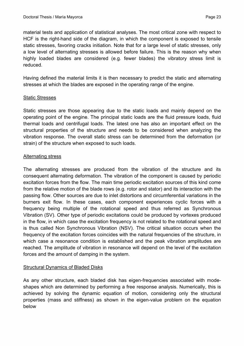
1E Figure 1-5: Beam mode-shapes and nomenclature

The free response mode-shapes of bladed disks can be considered as a combination of disk-alone and blade-alone mode-shapes. The nomenclature often used to refer to different blade mode-shapes is analogue to beam like modes and are classified depending on the number of inflection lines (1st, 2nd, etc.) and their orientation with respect to the blade (bending or flexion F, torsion T and edge wise bending E) as illustrated in Figure 1-5. In general, the low frequency blade mode-shapes are 1st bending (1F), 1st torsion (1T) and 2nd flexion (2F).

+ -

+ -

+-

1 nd 2 nd

Figure 1-6: Disk mode-shapes and nomenclature

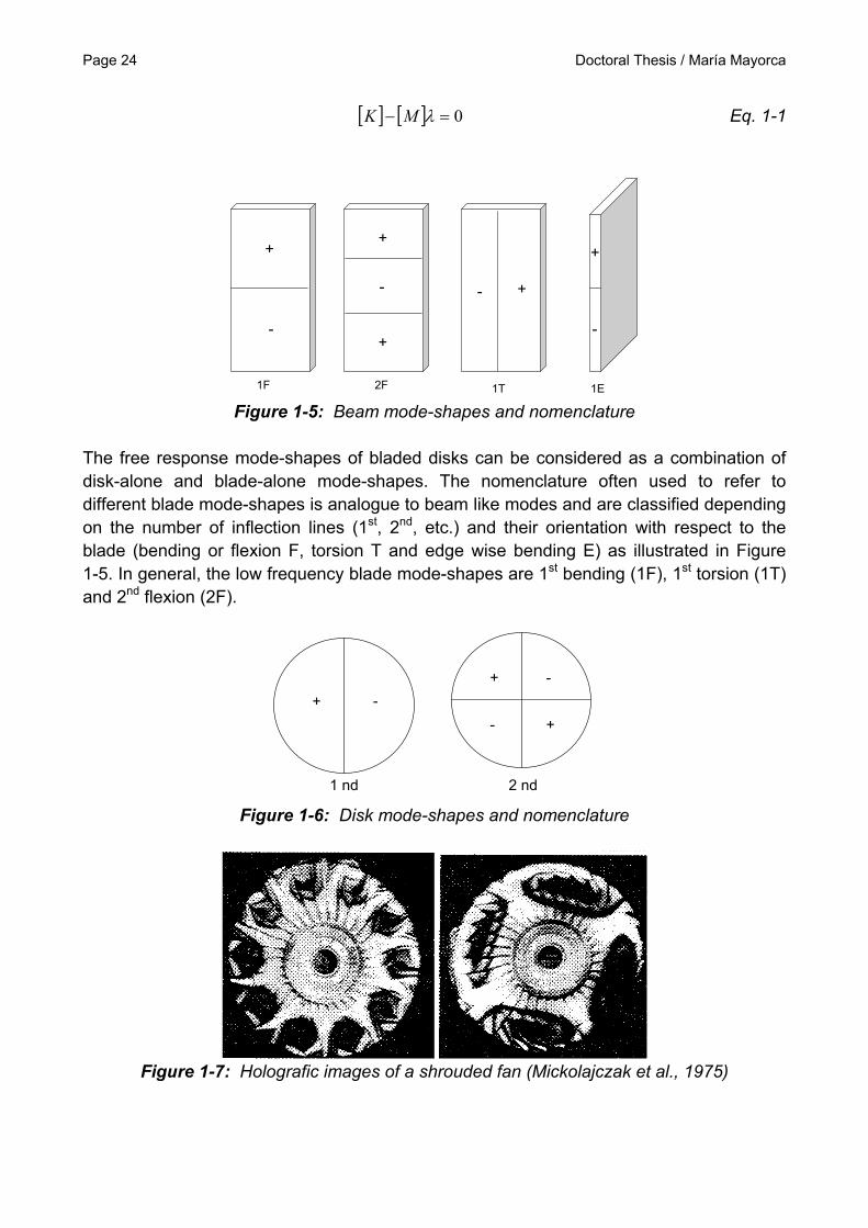
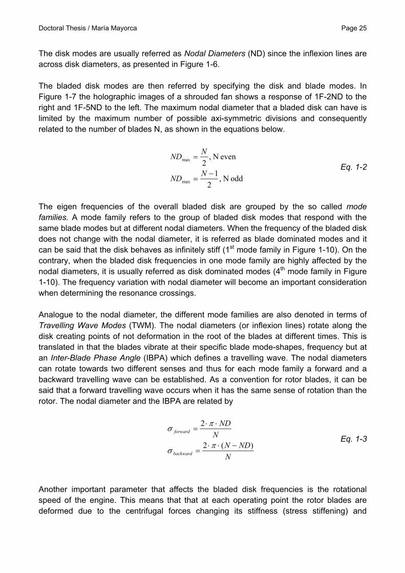
Figure 1-7: Holografic images of a shrouded fan (Mickolajczak et al., 1975)


The disk modes are usually referred as Nodal Diameters (ND) since the inflexion lines are across disk diameters, as presented in Figure 1-6.

The bladed disk modes are then referred by specifying the disk and blade modes. In Figure 1-7 the holographic images of a shrouded fan shows a response of 1F-2ND to the right and 1F-5ND to the left. The maximum nodal diameter that a bladed disk can have is limited by the maximum number of possible axi-symmetric divisions and consequently related to the number of blades N, as shown in the equations below.

odd N ,2

1

even N ,2

max

max

NND

NND

Eq. 1-2

The eigen frequencies of the overall bladed disk are grouped by the so called mode families. A mode family refers to the group of bladed disk modes that respond with the same blade modes but at different nodal diameters. When the frequency of the bladed disk does not change with the nodal diameter, it is referred as blade dominated modes and it can be said that the disk behaves as infinitely stiff (1st mode family in Figure 1-10). On the contrary, when the bladed disk frequencies in one mode family are highly affected by the nodal diameters, it is usually referred as disk dominated modes (4th mode family in Figure 1-10). The frequency variation with nodal diameter will become an important consideration when determining the resonance crossings. Analogue to the nodal diameter, the different mode families are also denoted in terms of Travelling Wave Modes (TWM). The nodal diameters (or inflexion lines) rotate along the disk creating points of not deformation in the root of the blades at different times. This is translated in that the blades vibrate at their specific blade mode-shapes, frequency but at an Inter-Blade Phase Angle (IBPA) which defines a travelling wave. The nodal diameters can rotate towards two different senses and thus for each mode family a forward and a backward travelling wave can be established. As a convention for rotor blades, it can be said that a forward travelling wave occurs when it has the same sense of rotation than the rotor. The nodal diameter and the IBPA are related by

N

NDNN

ND

backward

forward

)(2

2

Eq. 1-3

Another important parameter that affects the bladed disk frequencies is the rotational speed of the engine. This means that that at each operating point the rotor blades are deformed due to the centrifugal forces changing its stiffness (stress stiffening) and


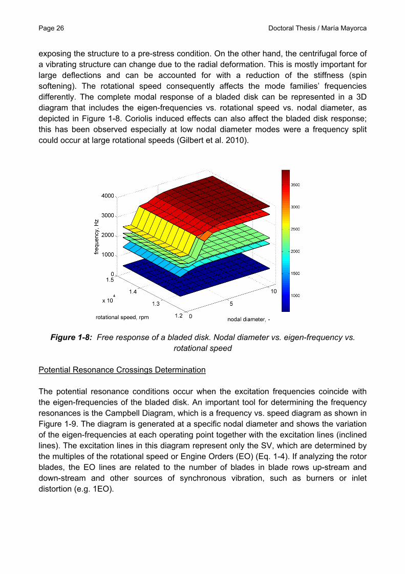
exposing the structure to a pre-stress condition. On the other hand, the centrifugal force of a vibrating structure can change due to the radial deformation. This is mostly important for large deflections and can be accounted for with a reduction of the stiffness (spin softening). The rotational speed consequently affects the mode families’ frequencies differently. The complete modal response of a bladed disk can be represented in a 3D diagram that includes the eigen-frequencies vs. rotational speed vs. nodal diameter, as depicted in Figure 1-8. Coriolis induced effects can also affect the bladed disk response; this has been observed especially at low nodal diameter modes were a frequency split could occur at large rotational speeds (Gilbert et al. 2010).

Figure 1-8: Free response of a bladed disk. Nodal diameter vs. eigen-frequency vs.

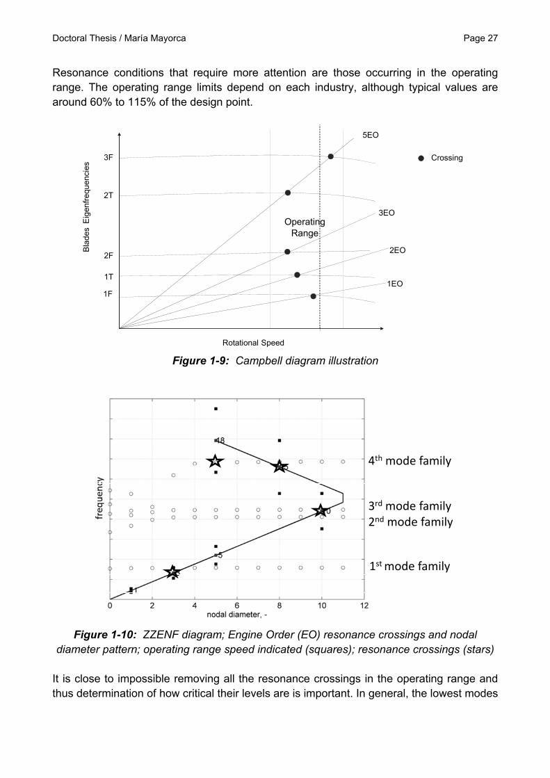
rotational speed Potential Resonance Crossings Determination The potential resonance conditions occur when the excitation frequencies coincide with the eigen-frequencies of the bladed disk. An important tool for determining the frequency resonances is the Campbell Diagram, which is a frequency vs. speed diagram as shown in Figure 1-9. The diagram is generated at a specific nodal diameter and shows the variation of the eigen-frequencies at each operating point together with the excitation lines (inclined lines). The excitation lines in this diagram represent only the SV, which are determined by the multiples of the rotational speed or Engine Orders (EO) (Eq. 1-4). If analyzing the rotor blades, the EO lines are related to the number of blades in blade rows up-stream and down-stream and other sources of synchronous vibration, such as burners or inlet distortion (e.g. 1EO).


Resonance conditions that require more attention are those occurring in the operating range. The operating range limits depend on each industry, although typical values are around 60% to 115% of the design point.

Operating Range

Bla

des

Eig

enfr

eque

ncie

s

1EO

2EO

3EO

5EO

1F

2F

1T

Rotational Speed

2T

3F Crossing

Figure 1-9: Campbell diagram illustration

1st mode family

2nd mode family3rd mode family

4th mode family

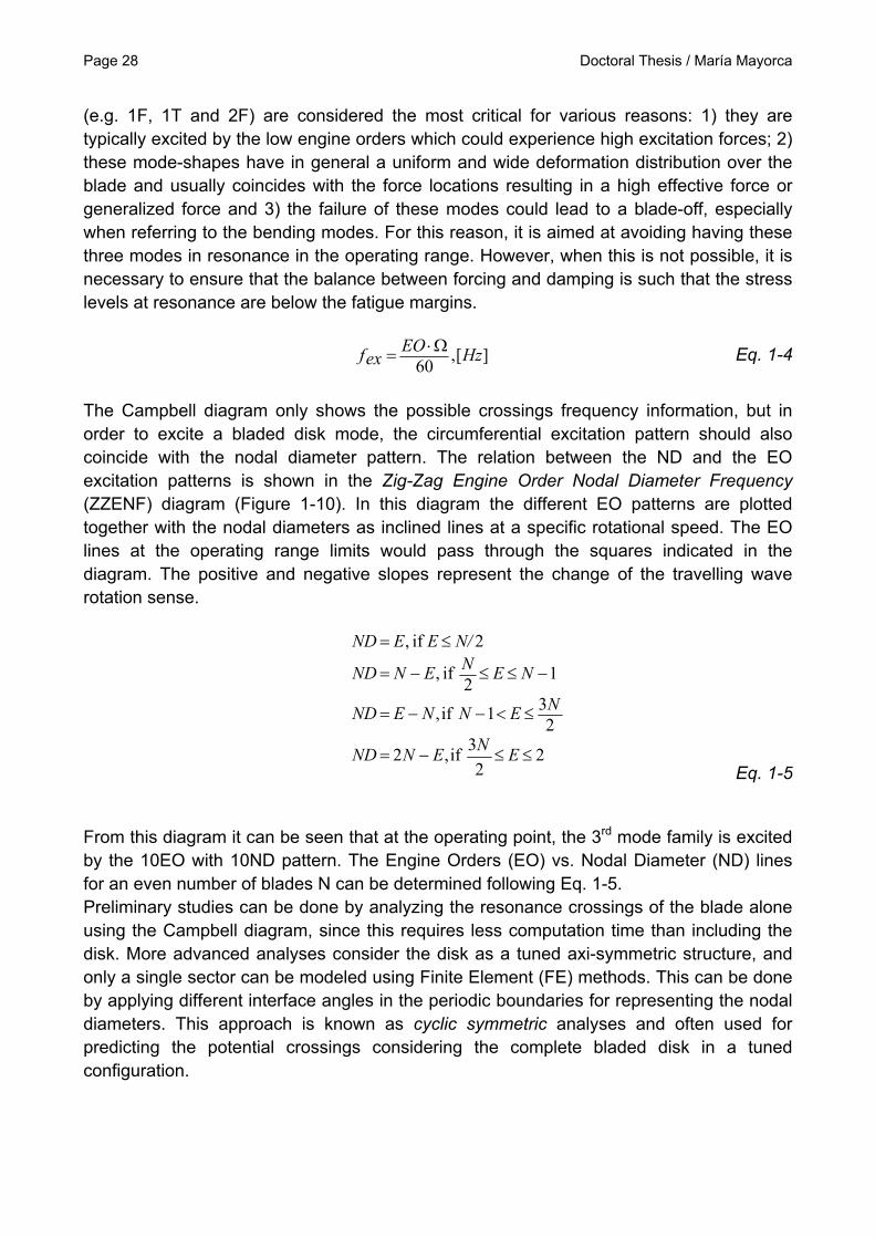
Figure 1-10: ZZENF diagram; Engine Order (EO) resonance crossings and nodal

diameter pattern; operating range speed indicated (squares); resonance crossings (stars)

It is close to impossible removing all the resonance crossings in the operating range and thus determination of how critical their levels are is important. In general, the lowest modes


(e.g. 1F, 1T and 2F) are considered the most critical for various reasons: 1) they are typically excited by the low engine orders which could experience high excitation forces; 2) these mode-shapes have in general a uniform and wide deformation distribution over the blade and usually coincides with the force locations resulting in a high effective force or generalized force and 3) the failure of these modes could lead to a blade-off, especially when referring to the bending modes. For this reason, it is aimed at avoiding having these three modes in resonance in the operating range. However, when this is not possible, it is necessary to ensure that the balance between forcing and damping is such that the stress levels at resonance are below the fatigue margins.

][,60

HzEOexf Eq. 1-4

The Campbell diagram only shows the possible crossings frequency information, but in order to excite a bladed disk mode, the circumferential excitation pattern should also coincide with the nodal diameter pattern. The relation between the ND and the EO excitation patterns is shown in the Zig-Zag Engine Order Nodal Diameter Frequency (ZZENF) diagram (Figure 1-10). In this diagram the different EO patterns are plotted together with the nodal diameters as inclined lines at a specific rotational speed. The EO lines at the operating range limits would pass through the squares indicated in the diagram. The positive and negative slopes represent the change of the travelling wave rotation sense.

22

3 if,2

231 if,

12

if ,

2if ,

EN

ENND

NENNEND

NENENND

N/ EEND

Eq. 1-5

From this diagram it can be seen that at the operating point, the 3rd mode family is excited by the 10EO with 10ND pattern. The Engine Orders (EO) vs. Nodal Diameter (ND) lines for an even number of blades N can be determined following Eq. 1-5. Preliminary studies can be done by analyzing the resonance crossings of the blade alone using the Campbell diagram, since this requires less computation time than including the disk. More advanced analyses consider the disk as a tuned axi-symmetric structure, and only a single sector can be modeled using Finite Element (FE) methods. This can be done by applying different interface angles in the periodic boundaries for representing the nodal diameters. This approach is known as cyclic symmetric analyses and often used for predicting the potential crossings considering the complete bladed disk in a tuned configuration.


Excitation Forces Once the potential resonance crossings are localized it is necessary determining if their vibration amplitude leads to HCF risk. This can be measured during the engine tests, but in case the resonance levels are above permissible, the costs would be extremely high and long iterations are required to reach a new design that matches both the aerodynamics and the structural dynamics goals. For this reason, it has become a common practice to predict the unsteady excitation forces through Computational Fluid Dynamics (CFD) computations. The most accurate analyses require the solution of the 3D Unsteady Navier Stokes equations for resolving the blade row interaction phenomena. These computations require a large amount of computational effort and several domain reduction methods have been proposed. The most common one is the chorochronic method, in which it is assumed that the flow is periodic in time and space and thus the multi-stage calculations can be reduced to including one single passage by blade row.

Flow

Ω

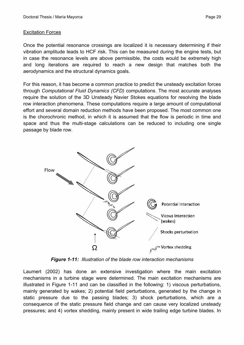
Figure 1-11: Illustration of the blade row interaction mechanisms Laumert (2002) has done an extensive investigation where the main excitation mechanisms in a turbine stage were determined. The main excitation mechanisms are illustrated in Figure 1-11 and can be classified in the following: 1) viscous perturbations, mainly generated by wakes; 2) potential field perturbations, generated by the change in static pressure due to the passing blades; 3) shock perturbations, which are a consequence of the static pressure field change and can cause very localized unsteady pressures; and 4) vortex shedding, mainly present in wide trailing edge turbine blades. In


practice, these mechanisms appear all together and result in a final unsteady pressure distribution on the blade surface. In analyses performed by Lee and Feng (2003) in a multi-stage compressor, it was determined that the peak-to-peak unsteady force amplitudes due to the viscous interactions (wakes) were of an order of 10%-15% of the peak-to-peak unsteady loading, being the remaining 85% to 90% attributed to potential field interactions. The unsteady pressures can then be Fourier transformed in order to determine the different harmonic contributions, including the excitation frequencies and distributed harmonic forces associated. The interaction of the excitation mechanisms will affect not only the absolute distributed force but also the blade surface relative excitation phase. Damping The other important parameter in the solution of the dynamic equation is the damping, which in turn will regulate the maximum responding amplitude at a resonance condition. The overall system damping in bladed disks is the sum of different damping contributions and can be classified in mechanical damping (friction and material damping) and aerodynamic damping.

The damping contributions can be expressed in terms of the critical damping ratio (Eq. 1-6) and is related to the ratio between the actual damping and the critical damping of the system. If considering the peak damped response, it is also related to the difference in

frequencies at either side of the natural frequency nf at half-power. Other notations are

also used such as amplitude factor Q, loss factor and the logarithmic decrement , which relation is presented in Eq. 1-7.

ncrit f

f

mk

c

c

c

22

Eq. 1-6

Q

2

1

22 Eq. 1-7

In bladed disks, one major source of damping is from friction. Friction damping sources can be from under platform dampers, shrouds or from fir-tree dry friction. The amount of friction damping depends on the inter-connections configuration, the rotational speed and the mode-shapes responding. For a part-span shroud values loss factor could be in the range of 0.0052 (torsion modes) to 0.056 (flexion modes), as summarized by Srinivasan (1997). The main challenges of predicting the friction damping is that it is not linear with the vibration amplitude, having also a stick-slip behavior. When the contact surfaces “stick” there is no relative motion between them and thus there is no friction, opposite to when they “slip”. Furthermore, the frequency can change due to an additional added stiffness


effect due to the dampers. For these reasons, more complex non-linear prediction models are necessary. Petrov and Ewins (2003) apply multi-harmonic models as well as large scale finite elements for the prediction of the sick-slip transitions. Corral (2008) has presented a simple micro-slip model (only a fraction of the contact surface is sliding) including a fir-tree dry friction model. The latter is applied in low pressure turbines, considering that for small amplitudes the energy dissipated due to friction is proportional to the vibration amplitude to the power of n (where n>2, typically 3). Blisks, on the other hand, being built from a single structure, do not have any friction damping at the blade to disk connections. For this reason, the only sources of damping are material and aerodynamic damping. The contribution from the blade materials (titanium based and Nickel-based alloys) to the overall damping is most often negligible, with loss factors around 0.0003 (1st and 2nd bending) and 0.0001 (1st torsion) (Srinivasan 1997), being up to 2 order of magnitudes lower to friction damping. More recent measured values of material damping on compressor blades have been reported by Zhai et al. (2011), with ranges of 0.04%-0-07% logarithmic decrement. The only contributor left is the aerodynamic damping, which is generated by the flow unsteady pressures from the blades vibration. This kind of damping depends not only on the mode-shape, but also on the operating point conditions, frequency of oscillation and inter-blade phase angle. The aerodynamic damping loss factors could reach values up to 0.02, having similar order of magnitudes than the friction damping. One particularity of this kind of damping is that it could become negative, and contrary to reducing the vibration amplitudes it would induce a self-excited condition where the vibration amplitude increases rapidly with imminent failure of the complete engine. The negative aerodynamic damping condition is referred as flutter and is treated in separated stability analyses.

1.2.2. Stability and Aerodynamic Damping

Aerodynamic damping is a phenomenon that occurs as a consequence of the blade vibration and its interaction with the flow. Prediction of the aerodynamic damping is of great relevance in aeromechanics for two main reasons: 1) the positive damping contribution is essential in order to regulate the vibration amplitudes at resonance conditions. This is particularly essential in blisk forced response analyses; and 2) the aerodynamic damping can become negative and if not compensated by mechanical damping, it can lead to a flutter condition which needs to be absolutely avoided. Stability Key Parameters A first indicator of flutter margins is the reduced frequency (k), which is the ratio of the frequency of oscillation (f) and blade chord (c) over the flow velocity (u) (Eq. 1-8). It can be understood as the time a particle needs to travel the chord of the blade (t) and the period of blade oscillation. This parameter indicates the unsteadiness of the flow. Small values of k indicate the flow is quasi-steady and for large values of k the unsteadiness dominates. A


k value of 1 implies that both quasi-steady and unsteady effects could be present. Increasing the flow speed at a fixed vibration frequency increases the flutter risk and thus a critical reduced frequency value can be defined as the minimum reduced frequency at which flutter would occur. In turbomachinery, reported values of flutter occurrences reduced frequencies are in the range of 0.4 to 0.7 (Srivasnava 1997).

ufc

Ttk

2 Eq. 1-8

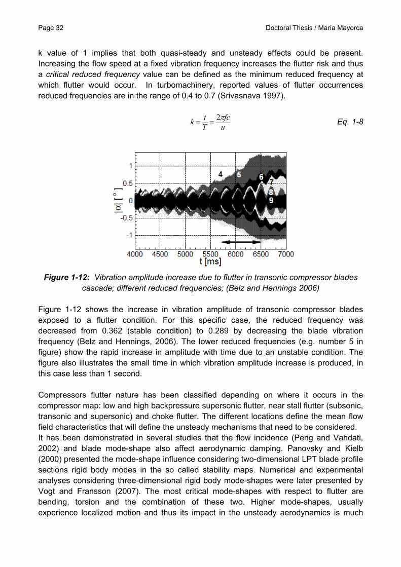
Figure 1-12: Vibration amplitude increase due to flutter in transonic compressor blades

cascade; different reduced frequencies; (Belz and Hennings 2006) Figure 1-12 shows the increase in vibration amplitude of transonic compressor blades exposed to a flutter condition. For this specific case, the reduced frequency was decreased from 0.362 (stable condition) to 0.289 by decreasing the blade vibration frequency (Belz and Hennings, 2006). The lower reduced frequencies (e.g. number 5 in figure) show the rapid increase in amplitude with time due to an unstable condition. The figure also illustrates the small time in which vibration amplitude increase is produced, in this case less than 1 second. Compressors flutter nature has been classified depending on where it occurs in the compressor map: low and high backpressure supersonic flutter, near stall flutter (subsonic, transonic and supersonic) and choke flutter. The different locations define the mean flow field characteristics that will define the unsteady mechanisms that need to be considered. It has been demonstrated in several studies that the flow incidence (Peng and Vahdati, 2002) and blade mode-shape also affect aerodynamic damping. Panovsky and Kielb (2000) presented the mode-shape influence considering two-dimensional LPT blade profile sections rigid body modes in the so called stability maps. Numerical and experimental analyses considering three-dimensional rigid body mode-shapes were later presented by Vogt and Fransson (2007). The most critical mode-shapes with respect to flutter are bending, torsion and the combination of these two. Higher mode-shapes, usually experience localized motion and thus its impact in the unsteady aerodynamics is much


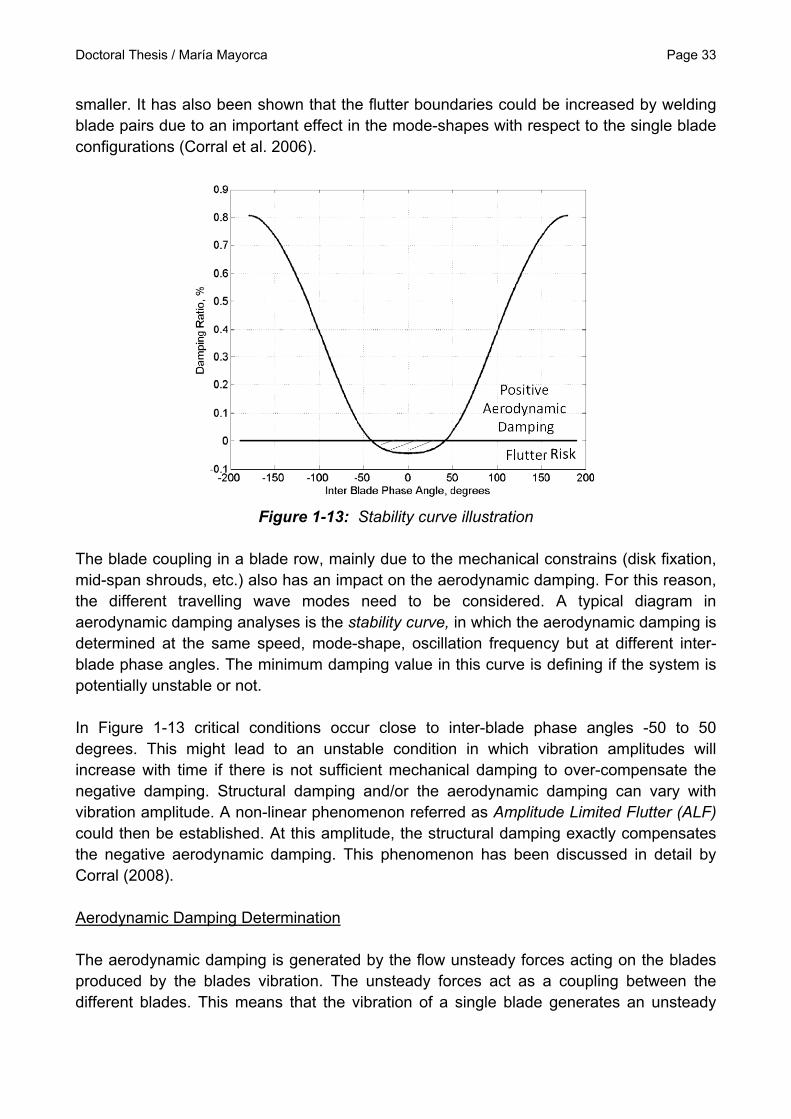
smaller. It has also been shown that the flutter boundaries could be increased by welding blade pairs due to an important effect in the mode-shapes with respect to the single blade configurations (Corral et al. 2006).

Figure 1-13: Stability curve illustration

The blade coupling in a blade row, mainly due to the mechanical constrains (disk fixation, mid-span shrouds, etc.) also has an impact on the aerodynamic damping. For this reason, the different travelling wave modes need to be considered. A typical diagram in aerodynamic damping analyses is the stability curve, in which the aerodynamic damping is determined at the same speed, mode-shape, oscillation frequency but at different inter-blade phase angles. The minimum damping value in this curve is defining if the system is potentially unstable or not. In Figure 1-13 critical conditions occur close to inter-blade phase angles -50 to 50 degrees. This might lead to an unstable condition in which vibration amplitudes will increase with time if there is not sufficient mechanical damping to over-compensate the negative damping. Structural damping and/or the aerodynamic damping can vary with vibration amplitude. A non-linear phenomenon referred as Amplitude Limited Flutter (ALF) could then be established. At this amplitude, the structural damping exactly compensates the negative aerodynamic damping. This phenomenon has been discussed in detail by Corral (2008). Aerodynamic Damping Determination The aerodynamic damping is generated by the flow unsteady forces acting on the blades produced by the blades vibration. The unsteady forces act as a coupling between the different blades. This means that the vibration of a single blade generates an unsteady


force field (or influence) on the surface of neighbor blades. The influence of the vibration of a single blade on another can be expressed in terms of complex influence coefficients. For small perturbations, the influence of the different blades superimposes linearly (Hanamura et al. 1980) and thus one can express the overall complex force at a specific inter-blade phase angle in relation to the different blade influences, as shown in Eq. 1-9. The subscripts n and m denote the influence of the vibration of blade n on blade m.

2

2

),,(,ˆ),,(,ˆ

N

Nn

niezyxmnicFzyxm

twmF Eq. 1-9

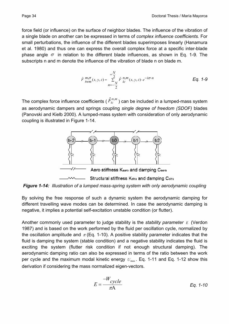
The complex force influence coefficients (mn

icF ,ˆ ) can be included in a lumped-mass system

as aerodynamic dampers and springs coupling single degree of freedom (SDOF) blades (Panovski and Kielb 2000). A lumped-mass system with consideration of only aerodynamic coupling is illustrated in Figure 1-14.

Figure 1-14: Illustration of a lumped mass-spring system with only aerodynamic coupling By solving the free response of such a dynamic system the aerodynamic damping for different travelling wave modes can be determined. In case the aerodynamic damping is negative, it implies a potential self-excitation unstable condition (or flutter). Another commonly used parameter to judge stability is the stability parameter E (Verdon 1987) and is based on the work performed by the fluid per oscillation cycle, normalized by the oscillation amplitude and (Eq. 1-10). A positive stability parameter indicates that the fluid is damping the system (stable condition) and a negative stability indicates the fluid is exciting the system (flutter risk condition if not enough structural damping). The aerodynamic damping ratio can also be expressed in terms of the ratio between the work per cycle and the maximum modal kinetic energy maxU . Eq. 1-11 and Eq. 1-12 show this

derivation if considering the mass normalized eigen-vectors.

AcycleW

E

Eq. 1-10


max4 UcycleW

Eq. 1-11

2

2)Im(2

2max

21

222

1max)cos(22

2

1max

)cos()(

)sin()(

2)(2

1max

mass modal :

amplitudevector -eigen normalized mass maximum :

U

bm

bmtbmU

tbtX

tbtX

tXmU

m

b

Eq. 1-12

There are different assumptions when predicting aerodynamic damping by using the SDOF system described above: 1) the mode families are well separated in frequency such no interaction between mode families is established; 2) the magnitude of the unsteady forces varies linearly with the oscillation amplitude; and 3) the mode-shape is not changing due to the unsteady forces influence. These assumptions are in general valid for small vibration amplitudes (assumption 2) and high blade-to-air mass ratio (assumptions 1 and 3). Previous studies (Gerolymos 1993 and Mårtensson et al. 2008) have shown that when two blade mode families interact (e.g. bending and torsion interaction), the aerodynamic damping predicted can be of considerable difference as for the one predicted for a single mode family. Fan and compressor blade designs are today pushed towards lighter and twisted blades and exposed to larger aerodynamic loads (e.g. open rotors). This implies a reduction of the mass ratio in favor of the possibility of mode family interaction. Clark et al. (2009) proposed a methodology for determining when a possibility of mode interaction flutter is present. This method determines a critical mass ratio below which flutter can occur as a function of the frequency and solidity of the blade, which could serve as an indicator of when a more advanced method should be considered.

1.2.3. Mistuning

Due to manufacturing tolerances, wear or Foreign Object Damage (FOD), bladed disks are usually not axi-symmetric (or tuned) and instead have a mistuning level. In the literature, mistuning due to change in structural properties (e.g.: mass or stiffness) is referred as frequency or structural mistuning. Typical values of the frequency mistuning


are around +/-2% deviations from the tuned blade frequency. One of the consequences of this kind of mistuning is that the travelling wave mode is broken and a frequency split is experienced. This means that each blade can be at resonance at different rotational speeds. The frequency split can also cause that mode families interact. This could be the case in blade designs with mode families with nodal diameters having close frequencies (veerings). In only structurally coupled analysis (no aerodynamic coupling), it has been shown that structural mistuning causes the energy to concentrate in few blades (mode localization) and thus these blades feature an amplitude magnification compared to the tuned structure (Bladh et al. 2000). This effect is highly detrimental with respect to HCF, lowering the margin to the allowable alternating stress. A first estimator of the maximum amplitude magnification due to mistuning is related to the number of blades (Whitehead 1998) as shown in Eq. 1-13. A further study by Han et al. (2007) related the maximum amplification factor to the amount of damping in bladed disks, concluding that the upper bound consistent with Eq. 1-13 occurred at low damping ratios and decreased with increasing damping ratios. It was also noted that the damping ratio at which the upper bound occurred depended also on the resonance condition studied. Using the upper bound considering only the number of blades can be over-conservative and thus more detailed analyses are necessary for each specific setup.

2

1max

NA

Eq. 1-13

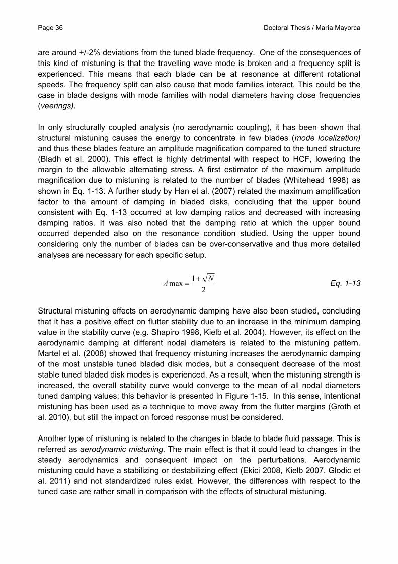
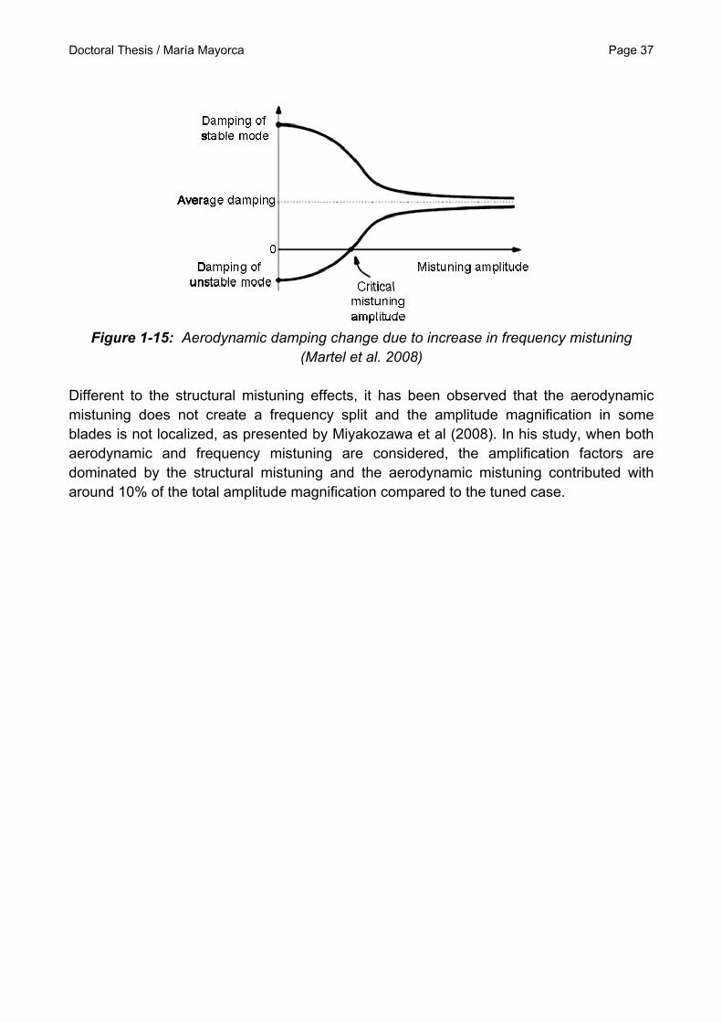
Structural mistuning effects on aerodynamic damping have also been studied, concluding that it has a positive effect on flutter stability due to an increase in the minimum damping value in the stability curve (e.g. Shapiro 1998, Kielb et al. 2004). However, its effect on the aerodynamic damping at different nodal diameters is related to the mistuning pattern. Martel et al. (2008) showed that frequency mistuning increases the aerodynamic damping of the most unstable tuned bladed disk modes, but a consequent decrease of the most stable tuned bladed disk modes is experienced. As a result, when the mistuning strength is increased, the overall stability curve would converge to the mean of all nodal diameters tuned damping values; this behavior is presented in Figure 1-15. In this sense, intentional mistuning has been used as a technique to move away from the flutter margins (Groth et al. 2010), but still the impact on forced response must be considered. Another type of mistuning is related to the changes in blade to blade fluid passage. This is referred as aerodynamic mistuning. The main effect is that it could lead to changes in the steady aerodynamics and consequent impact on the perturbations. Aerodynamic mistuning could have a stabilizing or destabilizing effect (Ekici 2008, Kielb 2007, Glodic et al. 2011) and not standardized rules exist. However, the differences with respect to the tuned case are rather small in comparison with the effects of structural mistuning.


Figure 1-15: Aerodynamic damping change due to increase in frequency mistuning

(Martel et al. 2008)

Different to the structural mistuning effects, it has been observed that the aerodynamic mistuning does not create a frequency split and the amplitude magnification in some blades is not localized, as presented by Miyakozawa et al (2008). In his study, when both aerodynamic and frequency mistuning are considered, the amplification factors are dominated by the structural mistuning and the aerodynamic mistuning contributed with around 10% of the total amplitude magnification compared to the tuned case.



2. STATE OF THE ART IN AEROMECHANICS OF TURBOMACHINERY

2.1. Aeromechanical Design

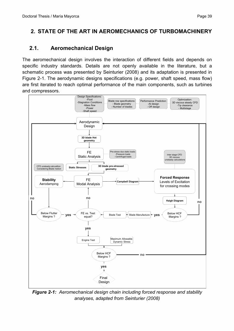
The aeromechanical design involves the interaction of different fields and depends on specific industry standards. Details are not openly available in the literature, but a schematic process was presented by Seinturier (2008) and its adaptation is presented in Figure 2-1. The aerodynamic designs specifications (e.g. power, shaft speed, mass flow) are first iterated to reach optimal performance of the main components, such as turbines and compressors.

Optimization:3D viscous steady CFD

-Tip clearance- Multistage

Design Specifications:-Fluid

-Stagnation Conditions-Mass flow

-Power-Shaft speed

Blade row specifications:- Blade geometry

- Number of blades

Performance Prediction:-At design

- Off design

3D blade Hot geometry

Pre-stress due static loads:-Pressure loads

- Centrifugal loads

3D blade pre-stressedgeometry

Static Stresses

AerodynamicDesign

FEStatic Analysis

FEModal Analysis

Campbell Diagram

Maximum Allowable Dynamic Stress

Blade ManufactureBlade Test

Engine Test

FE vs. Test equal?

Below HCF Margins ?

Final Design

yes

yes

Forced ResponseLevels of Excitationfor crossing modes

Inter stage CFD 3D viscous

unsteady calculations

Haigh Diagram

Below HCF Margins ?

yes

no

nono

StabilityAerodamping

CFD unsteady calcualtionConsidering Blade motion

Below FlutterMargins ? yes

no

Figure 2-1: Aeromechanical design chain including forced response and stability

analyses, adapted from Seinturier (2008)


Once the aerodynamic performance required is reached, it is necessary to ensure that the engine is structurally capable: 1) the excitation levels need to be below the fatigue margins and 2) the operating points need to be far away from the flutter margins. These two points can be answered after the engine tests, but if a failure occurs, the design loop might need to be re-started from the aerodynamic design, meaning high effort and cost. For this reason, including the numerical predictions of both forced response and stability in the design chain is a growing interest. Furthermore, there has been a great development of numerical models that aim at reaching aeromechanical standardized procedures in feasible time but maintaining accuracy.

2.1.1. Fluid Dynamic Unsteady Calculation Models

For predicting the fluid excitation levels in a forced response analysis, multi-stage unsteady calculations are necessary. Due the large computational effort that implies resolving the full annulus stages, much effort has been directed towards reduction models. Erdos and Alzner (1977) developed a method which only requires one stage passage for the calculation, where the flow solution is stored at pitchwise boundaries during a blade passing period and applied as boundary conditions for the following period. This is also known as chorochronic periodicity methods. One drawback of this method is that it takes a long time to reach periodic convergence. A similar method, applied to two-dimensional Euler equations was presented by Fransson (1986), in which only a blade passage is calculated, in which an inter-blade phase angle is applied as boundary conditions. The methods were applied for stability analysis (i.e. flutter) rather than for forced response calculation. A similar approach is the phase-shifted periodic boundary condition method implemented in an Euler solver by He (1992), also known as the “generalized correction method”. In this model the solution of a single-passage with multiple perturbations is obtained by identifying the perturbations at the periodic boundaries by their own phase-shifted periodicities and approximated by Fourier series. This method allows storing only the Fourier components. One of the limitations of this model is that is based on the assumption that the flow is periodic in time and other non-linear viscous excitation mechanisms such as vortex shedding are not captured. A chorochronic periodicity method which captures the non-linear behavior of the wakes has been presented by Olausson et al. (2007) and works in three steps: first it samples values at each periodic side to update Fourier coefficients; then evaluates the Fourier series at the corresponding phased shifted time between the sides (time shift) and uses the rotated and shifted variables in the other side; finally the Fourier representation is evaluated again and used to damp out non periodic flow phenomena in the cells of the sampling. The method was partly validated against a frequency domain linearized Navier-Stokes equations solver method. Another approach which does not assume temporal periodicity is the time inclined method presented by Giles (1990), where the computational time is inclined by a transformation of


the governing equations in order to fulfill the phase lagged boundary conditions. This approach has been used widely including the 3D viscous unsteady calculations by Laumert et al. (2002) for rotor-stator interaction predictions. In this technique the number of nodes that must be retained grows if more blade rows are involved. With multiple stages the computational effort grows and the reduction relative to a full annulus model is reduced. Limitations of this method are that it is difficult to apply if time is inclined in more than one spatial direction; it is not stable when the row blade number ratio is higher than unity and is limited to only two blade rows.

Another reduction method is based on decreasing the domain size by modeling stages sectors with equal net pitch fulfilling the circumferential periodicity. The advantage of this approach is that the solver boundary condition treatment does not need to be modified. In general, compressors and turbines have non-reducible fractions between the number of stator and rotor blades and thus scaling the blade passages to fit divisible blade counts is necessary. Rai and Madavan (1990) demonstrated this technique. Clark et al. (2000) and Schmitz et al. (2006) have addressed the effect of scaling in the analysis of turbine forced response. Whereas Clark et al. (2000) focused on the prediction accuracy of unsteady pressure, it was concluded that already small amount of scaling might have comparatively large effects. On the other hand, Schmitz et al. (2006) concluded scaling to be a valid method for assessing the aerodynamic forcing of adjacent blade rows. An investigation on the influence of including multi-stages on compressors forced response calculation was performed by Vahdati (2007), where non-linear time accurate Navier Stokes calculations were performed with five stages. It was concluded that for the prediction of the main blade-passing force frequency, two blade rows computations might produce accurate results. Nevertheless, the low engine harmonics can also become important and in order to capture them multi-stage calculations are necessary. It is highlighted that the lack of mesh resolution for including multiple rows in the unsteady CFD calculations can also jeopardize the accuracy of the results. It was recommended then to include stator/rotor/stator configurations instead of single stage ones.

2.1.2. Structural Models

The main challenge in the structural field is including the mistuning effects, both on forced response and stability. Mistuning modeling requires solving the dynamic equation of motion for the complete full annulus model. Since the mistuning patterns are not known, probabilistic analyses (e.g. Monte Carlo simulations) are performed and thus it is required reducing the domain size. For this reason, different Reduced Order Models (ROM) have been developed and adapted for different aeromechanical prediction tasks. The first models that were applied in turbomachinery mistuning predictions were those that did not consider the aerodynamic coupling. In this case, the forced response was performed considering only the disk connections or structural coupling.


One of these techniques is the Modal Decomposition (MD) and was applied by Yang and Griffin (2001), Bladh et al. (2001a, b) and Moyroud et al. (2002). Mistuned modes are represented in terms of a limited sum of subset of “nominal” system modes. The method is based on the assumption that any mistuned bladed disk mode shape can be represented has a linear combination of the bladed disk tuned modes. A subset of nominal modes is selected and thus increasing the number of modes in the subset increases the overall accuracy of the model. The method is more accurate for mode families that do not interact. Even when this method allows analyzing true bladed disk geometries, it has been considered mathematically complicated for providing physical insight into the mistuning problem (Feiner and Griffin 2002) and requiring a high amount of input data from the tuned assembly finite element analyses. Another ROM technique is the Component Mode Synthesis (CMS). This technique employs modes of the individual substructures instead of modes of the entire structure. A requirement is that the modes must be linearly independent and a complete set of modes should yield the exact solution as the FE original model. This method has been widely applied in turbomachinery having as substructures the disk (or disk sectors) and the blade by Yang and Griffin (1997), Castanier et al. (1997). Inside the CMS, the Craig and Bampton (1968) technique has been adapted to turbomachinery, having as main characteristic that two sets of modes are needed for representing the motion of each substructure: 1) a set of nominal dynamic modes of vibrations with the DOF at the component interfaces fixed and 2) a complete set of static constraints modes induced by successive unit deflection of each interfaces DOF while all other interface DOF are held fixed. This has been applied by Bladh et al. (2001), including mistuning on the blades sub-set. One limitation of the Craig and Bampton models is that it cannot represent large mistuning, as for example is the case of Foreign Object Damage (FOD). A reduction model that would allow large mistuning is the one proposed by Guyan (1965), in which the whole structure is defined in terms of selected master nodes. A basis of modes is created based on the static deformation of the structure due to the unitary deflection of each master node degree of freedom. The response can then be represented as a linear combination of the master nodes static modes. One of the advantages of this method is the simplicity of the mathematical implementation. Since it is based in the static characteristic of the system, the solution is exact for the static problem but results in an approximation for dynamic systems. In this case, the accuracy is dependent on the number of master nodes selection and location, being more suitable for lower modes. A comparison of the accuracy of both Craig Bampton and Guyan reduction applied on non-linear dampers was presented by Green (2006), concluding the Craig Bampton method would have a better accuracy for a larger range of mode-shapes. However, it is pointed out that the Guyan accuracy can increase by selecting a different number of master nodes and distribution and is suitable for including friction damping non-linear effects. An application of the Guyan reduction was recently presented by Zhai et al. (2011), where forced response mistuning analyses of the


first mode family of an industrial bladed disk compressor with considerations of aerodynamic coupling was assessed. A different approach has been developed by Feiner and Griffin (2002) and called the Fundamental Mistuning Model (FMM). It is applicable when only a mode family is excited and the strain energy of that family of modes is mainly in the blades. The mathematic application once the model is derived is similarly simple as the lumped mass system and yet be valid for real turbomachinery geometries. Fundamental mistuning parameters can be easily identified for parametric forced response predictions. It is based in the tuned bladed disk frequencies and the deviation of individual mistuned blade-alone frequencies to their tuned frequencies. The main restriction is that the mode family represented should have a close frequency (blade dominated modes) or in other words, considering an infinitely stiff disk. The FMM has been updated for flutter analysis including aerodynamic and structural coupling by Kielb et al. (2004). A further adaptation of the FMM has been performed by Martel et al. (2008) to the Asymptotic Mistuning Model (AMM) which also allows describing the effect of small mistuning on modes belonging to families exhibiting a non-small variation of the frequency mode family. Due the possibility of including aerodynamic coupling in both the AMM an FMM, these methods have given a good understanding of the mistuning effect on both amplitude magnification and aerodynamic damping. Using the AMM, it was shown that the aerodynamic damping responding to a specific nodal diameter vibration pattern could be affected by adding an intentional mistuning pattern that would couple the responding waves. Another method that includes the aerodynamic coupling effect was the one presented by Petrov (2009), in which sufficient FE tuned cyclic symmetric modes are first calculated, mistuning modeled by mass elements attached to nodes of the FE model, an in addition an aerodynamic matrix is included that represents the fluid coupling. This matrix is built from influence coefficients calculated in external CFD simulations for the tuned disk modes. This type of model permits the forced response predictions in a wide general manner, having the effects of mistuning on both the aerodynamic damping as well as in the structure mode localization. This is especially important in assemblies with low mechanical damping, such as blisks.

2.1.3. Fluid-structure Coupling

An overview of the different fluid-structure interaction approaches for forced response and flutter analysis have been presented by Moffatt and He (2005). A classification depending on the coupling strength of the fluid-structure interaction approach can be simplified to: decoupled, intermediate coupled and fully-integrated systems. In decoupled systems, the structure and flow behavior is assumed to be linear. Structural modes and frequencies, unsteady blade row interaction forces and aeroelastic forces are calculated separately. The following assumptions are considered: 1) structure vibration level (or amplitude) is linear with excitation level; 2) the aeroelastic damping forces are linear with vibration amplitude and 3) the oscillation mode shape is not affected by the aeroelastic forces. It is regularly accepted that mode-shapes remain unaffected for lightly-


damped blades or in other words, with high mass ratio. This is the case for the methods described above, were the fluid is solved separately from the structure. The intermediate coupling or partially-integrated schemes consider that the structure behaves linearly with the excitation but that the aeroelastic forces are not linear with vibration amplitude. An iterative process is then necessary: the forcing function and mode-shapes are calculated separately and a first aeroelastic damping is estimated. A new forcing function is calculated considering the aerodamping and new updated amplitudes and mode-shape obtained. A new aeroelastic computation is done. A new response is computed until convergence is reached. First iterations on the forced response of the analysis can be done considering only the blade alone and final iterations might be performed considering also the disk. In the coupled or fully-integrated scheme fluid and structural equations are solved simultaneously under the same numerical scheme. Nor the structure neither the aeroelastic forces are considered to be linear. At each time step the forces are applied on the blade surfaces (forcing function and aero forces together). The damping used to determine the response is only mechanical. An iterative integration is required: at each step the structure displacements are calculated and the flow path is modified. Then the unsteady pressure is modified, etc. The solution is reached when oscillation of the blade is stabilized. Fully-coupled methods based on both inviscid and viscous flow solvers have been used for flutter calculations by Silkowski et al. (2001) and Srivastava et al. (2002). In the later, investigation of the shock effect on the flutter initiation was conducted. Stall flutter initiation and development in compressors have also been studied with this kind of solvers, in which case Detached Eddy Simulations (DES) have also been integrated (IM et al. 2011). For forced response predictions, multi-stage models become important and implementing fully coupled schemes in regular design processes becomes highly costly. Sayma et al. (2000) applied coupled solvers for determination of the resonance response of IP and LP turbines. In this case the positive damping due to the vibration of the blade and its influence on the unsteady excitation mechanisms is solved in the coupled simulation. It was highlighted the low engine orders could be better predicted with a larger CFD mesh refinement for better solution of the viscous unsteadiness, and thus the coupled solver computational time would need to be increased even more. Some investigations have been performed regarding the accuracy of the different fluid-structure interaction methods. Tran and Liauzun (2006) showed agreement between a diversity of coupled and decoupled methods when calculating the aeroelastic stability of a transonic blade row. It was also highlighted that in the studied cases mode-shapes did not change due to the aerodynamic forces. On the other hand, in decoupled methods the CFD calculations were calculated only once and could be applied later for parametric studies by changing other structural parameters, as in mistuning predictions. Moffatt and He (2003) conducted studies of the influence of decoupled and fully coupled systems on the forced response amplitudes on a transonic fan; the coupled solutions were found to be strongly affected by a frequency shift due to the added mass effect of the vibration-induced aerodynamic damping forces. The decoupled method was shown to be insensitive to


frequency shift, maintaining resonance at the blade natural frequency and capturing the resonant peak with one solution. Due to the practicality and yet accurate predictions it was identified to be the best approach for blade-row interaction problems.

2.2. Accuracy in HCF predictions

The CFD codes development and the structural methods, as described above, have shown to become important tools for estimating specific phenomena in turbomachinery aeromechanics: determination of maximum amplitude magnifications, flutter margins determination, excitation levels at different engine orders, etc. However, it is not fully open in the literature what would be the accuracy expected while using these methods for predicting the overall fatigue risk. The main challenge in the validation of the aeromechanical chain numerical predictions is the complexity of obtaining clean experimental data that allows separating the different error sources at least in these main areas: 1) estimation of the excitation levels by CFD tools, 2) estimation of the aerodynamic damping by CFD tools, 3) estimation of the structural damping and 4) estimation of the structural model behavior, including mistuning. In an axial transonic turbine bladed disk, forced response predictions were presented by Green (1999). In this case, CFD calculations for the blade row interaction forces prediction as well as for aerodynamic damping were performed. However, aerodynamic damping was much smaller than the structural damping due to under-platform dampers, predicted considering non-linear models. The mean blade amplitude deviations from strain gauges correlated to the numerical predictions for the 1st and 2nd bending modes in resonance was around 30% (over-predicted) to 20% (under-predicted) respectively. In this case, the peak blade amplitude due to mistuning was not numerically estimated. An overview of the capability of the numerical tools in the aeromechanical chain was presented by Andersson et al. (2010). In this study, it was demonstrated how CFD blade row interaction could predict well the peak resonances in a turbine bladed disk as compared with tip timing measurements. This means that the relative excitation levels between the crossings in the operating range could be ranked. However, comparisons with the absolute maximum resonance amplitude predictions including structural and aerodynamic damping were not available. Another study was the one presented in the centrifugal compressor field by Ramakrishnan et al. (2011), were forced response analyses considering three blade rows interaction was performed using a Reynolds Averaged Navier-Stokes solver and results compared with experiments. It was concluded that the CFD analyses determines the nature of the impeller-return channel interaction with vane diffusers for low pressure ratios and mass flow, and determines most frequency content of the excitation. It is, nevertheless, highlighted that some acoustic modes were not captured by the CFD. On the other hand, no absolute error with respect to the possible absolute vibration amplitude prediction is given.


Another effort for validation of the aeromechanical design cycle was done by Zemp et al. (2011a and b), also in centrifugal compressors. Both unsteady pressures and resonance amplitudes (by strain gauges) were obtained experimentally at different inlet flow conditions. In this case, the damping ratios were measured. The numerical predictions were performed by using a commercial 3D unsteady Navier-Stoke solver and the damping considered applied from the test results. It was reported that the numerical predictions of the stress levels were under-predicted by all the cases, with factors of 3 and 4 lower with respect to the experiments. The differences in this study could be mainly attributed not only to the predictions of the excitation levels, but also to the absence of mistuning consideration. On the other hand, the test to prediction factor could also change if including the uncertainties due to numerical damping predictions, instead of using damping test data. The previous studies give an overview of the order of magnitude of the expected errors in the HCF design chain of bladed disks including large mechanical damping. Nevertheless, it is not very clear identifying which the main sources of numerical inaccuracies are. On the other hand, for blisks having aerodynamic damping as major source of damping, not much accuracy reports with respect to fatigue predictions are available in the open literature.


3. OBJECTIVES AND APPROACH

3.1. Objectives

The main objective of this work is the development, validation and application of a numerical tool for aeromechanical analyses, with estimation of the overall accuracy of the design chain compared to experimental results. Furthermore, the secondary objective is to propose a new method that includes the effect of mode-shape perturbation on the aeroelastic system. Under these objectives, four different sub-objectives are defined as follows:

1. Development of the numerical tool AROMA (Aeroelastic Reduced Order Modeling Analyses) for forced response and aerodynamic damping analyses including mistuning in a standardized manner

2. Quantification of a number of possible uncertainties in the numerical aeromechanical predictions of blisk assemblies

3. Application of the AROMA tool for the forced response prediction of an industrial

compressor blisk and comparisons with experiments

4. Development and application of a method for consideration of the aeroelastic response of mode-shapes different to the tuned in-vacuo ones

3.2. Approach

A summary of the main parts of the thesis is described as follows. The details of each section are explained in the corresponding chapter. Development and Validation of the Numerical Tool AROMA The numerical tool AROMA is developed in a user friendly interface (Matlab) which allows the application by different engineers in the design stage. The pre-processing consists on importing CFD results and FE structural data (mass and stiffness matrices) from external in-house or commercial tools, not being restrictive to one specific code. The AROMA solver assembles the CFD results with the FE model and uses a Reduced Order Model (ROM) in order to reduce the domain size allowing mistuning analyses both for forced response and aerodynamic damping analyses. The forced response results can be exported in the form of complex displacements for further stress assessment in a structural solver. A major strength of this approach is that the tool allows for parametric studies and could be used at different stages of the design chain, and is open to further


implementation of emerging methods. The validation of important tool capabilities with existing tools achieved by using simplified blisk assemblies and compared with existing FE solvers. Details of the AROMA tool description and validation are presented in chapters 4 and 5. Quantification of Numerical Uncertainties There are different sources of uncertainties in the overall chain, such as: mesh resolution and topology, turbulence models, structural damping estimation, transient solver type (time marching or linearized), model reduction approximations, FE-CFD data transfer, among others. The prediction errors are carried out in the overall chain and affect the final result. Three sources of numerical uncertainties have been investigated in detail in the current design chain for forced response analysis:

1) Fluid domain reduction in 3D unsteady blade row interaction CFD calculations by scaling. Its uncertainty is here quantified by parametric modification of the blade counts of a transonic compressor stage allowing reduced matching pitches. The unsteady forces are determined in all the cases and its effect on the generalized force quantified and compared with the full annulus model results.

2) Transfer of data between CFD and FE domains or mapping. Its uncertainty is here estimated by performing two different mapping methods: a) transferring CFD forces to the FE domain, b) transferring FE displacements to the CFD domain.

3) Finite Element domain reduction by Guyan condensation. Its uncertainty is estimated by the parametric selection of different number and distribution of master nodes on the compressor blade. The effect on frequency and mode-shape prediction is assessed by comparisons with the full blade model.

Point 1) above has been studied here in detail since the scaling approach could still be an industry standard method for aerodynamic forcing calculations due to not requiring specific treatment of the boundary conditions. In principle, most commercial tools for the solution of the unsteady aerodynamics would serve for this purpose. Estimating the errors introduced by this approach is of interest if it is used as part of the aeromechanical analysis. Point 2) is studied here since in un-coupled CFD-FE analyses, the mapping of the meshes would be a necessary step. Establishing the order of magnitude of the errors introduced would give an idea of the sensitivity of the mapping process with respect to other sources of uncertainties along the aeromechanical chain. Point 3) is performed since the Guyan reduction is a method implemented inside the AROMA tool for mistuning analyses.


It is important to highlight that many other parameters might also introduce different uncertainty errors but only the three above are considered here. Details of this analysis are presented in chapter 7. Forced Response Prediction of an Industrial Compressor Blisk with Comparisons with Experiments An industrial compressor blisk “Hulda” (Mårtensson et al. 2007) is used as test case. CFD steady and unsteady calculations are carried out at a resonance crossing of interest using a k-epsilon turbulence model. The excitation forces on the rotor blade due to blade row interaction are calculated. Furthermore, the aerodynamic damping forces due to blade motion are determined and considered as the only source of damping. For this application, the aerodynamic damping is estimated by considering the influence of only the mode family of interest and thus the SDOF approach for aerodynamic estimation is used. The AROMA tool is applied for the forced response calculation, including a statistical mistuning analysis. The final predicted amplitude is compared with experimental tip timing data. Two different operating conditions are considered, having the Variable Inlet Guide Vanes at two different setups: at 0º (nominal case) and at +30º. A discussion of the discrepancies obtained and detection of main sources of uncertainties in the aeromechanical chain are highlighted. Details of this analysis are presented in chapter 8. Development and Application of a Method for the Aeroelastic Response of Perturbed Modes To consider the effect of perturbed responding mode-shapes in the aeroelastic calculations a new method is proposed: the Multimode Least Square method (MLS). It is based on the determination of representative aerodynamic matrices (mass, stiffness and damping) to be included in the dynamic equation system. These matrices are determined having as input aerodynamic damping forces from blade motion CFD or experimental calculations of various mode-shapes. Different to the single degree of freedom approaches, the method is based on performing a least square fit of all mode-shapes aerodynamic forces, resulting on distributed influence coefficients aerodynamic matrices that can represent the aeroelastic behavior of responding mode-shapes different to the input ones. This approach allows for mode perturbation due to different sources (e.g. mistuning, coating damping, highly damped blades due to the aerodynamics, etc.). In addition, the Guyan reduction consistently with the structural model is implemented in order to reduce the domain size, being also applicable to parametric studies. The method is applied on a transonic compressor blade for stability and forced response analyses, including mistuning. Furthermore, its possible application on parametric studies is demonstrated. Details of these analyses are presented in chapter 9, whereas the governing equations are presented in section 4.3.



4. AEROELASTIC REDUCED ORDER MODELING ANALYSES (AROMA)

4.1. AROMA Philosophy

Computational Fluid Dynamics methods have had an extensive development both in the commercial market as well as in the form of in-house codes for specific industry needs. For particular applications there is a variety of requirements with regards of turbulence modeling, mesh generation, advection schemes, boundary conditions treatment, solver schemes (e.g. time marching or linearized), among other considerations that could be relevant for specific analyses. For this reason, the aeromechanical design chain should be flexible to different solver requirements, availability and keep up with industry standard procedures with regards of CFD design processes. Similarly is the case in the structural dynamics field and thus specific Finite Element tools are preferred and applied following design standards. The AROMA tool concept relies on the integration of relevant CFD and FE results for the analysis of aeromechanical problems at different levels in a standardized manner, and yet allowing flexibility on specific requirements on CFD and FE solvers. This means that it enables the possibility to perform parametric de-coupled analyses in turbomachinery components, not requiring as much computational effort as the fully coupled fluid-structure time marching methods. If necessary, iterative analyses can be performed in a partially coupled fashion. This could be the case when there are considerable changes of the oscillation frequency due to the aerodynamic coupling influence and/or mode-shape modification. AROMA is built considering as main users design engineers from different fields and thus keeping a high level of user-friendliness. It takes advantage of existing methods for stability and forced response analysis for preliminary design and also allows for mistuning considerations through Reduced Order Modeling (ROM) with or without aerodynamic coupling. Furthermore, a newly proposed method for consideration of mode-shape modification is implemented.

4.2. AROMA Structure

The work flow of AROMA consists on importing data from external fluid and structural solvers, fluid-structure data integration considering specific analysis needs, domain reduction, expansion to full annulus model, solution of forced response or stability analysis and export of the results for further stress assessment (in case of HCF). This process is illustrated in Figure 4-1. Pre-processing The Finite Element pre-stressed structural mass, stiffness and optionally damping matrices of a single blade or blisk sector(s) are imported. The CFD harmonic or time marching forces on the blade surface are also inputs to AROMA. In case of time-marching forces, a Fourier transformation is performed for each blade node surface in order to obtain distributed forces in the frequency domain. The forces can be obtained from blade row interaction and/or blade vibration unsteady forces CFD simulations. In case the scaling technic was applied for the blade row interaction calculations, a back-scaling of the


geometry and forces is performed in the frequency domain for each specific engine order of interest. Mapping of fluid-structure data For rotating components, the static displacements obtained in external structural solvers are imported for compatibility of cold to hot geometries. The transfer of fluid-structure data can be done in different manners:

1) Distributed fluid forces are transferred to the structural mesh by placing each CFD node force at its closest FE node. This is a conservative approach, in the sense that the total integrated force is preserved.

2) The mode-shapes are interpolated onto the CFD mesh by radial weighted average. The harmonic forces are projected into the interpolated amplitude normalized mode-shapes and the generalized force is obtained. This force is then applied as a point force at the maximum mode displacement location.

In the case of blade-row interaction calculations, forces are obtained directly from the CFD solvers. In the case of CFD aerodynamic damping calculations, pressures or forces can be imported to AROMA. Reduced Order Modeling The structural domain is reduced using the static condensation proposed by Guyan (1965). The master node selection can be performed in a parametric manner considering specified percentage of master nodes and distribution pattern with respect to mode-shapes from blade alone analyses. The number of disk interface master nodes can also be selected parametrically. Full annulus expansion The reduced sectors are then expanded to the full annulus model by the disk sectors interfaces coupling. Mistuning is modeled by imported sectors with different structural properties assembled in different circumferential patterns. For stability analyses or aero-coupled considerations the influence coefficient springs are assembled from the harmonic blade vibration CFD forces. The blade excitation forces can be applied specifying nodal diameter patterns. Solver The main analyses are modal analyses, forced response and stability analysis (or aerodynamic damping analysis) and achieved by solving the dynamic equation of motion in frequency domain. The stability curve is calculated by considering each blade as single degree of freedom coupled by blade vibration unsteady forces (i.e. aerodynamic springs). This method is here referred as the Single Degree of Freedom (SDOF) approach for aerodynamic damping estimation. Structurally coupled forced response analysis consider only linear damping, and thus non-linear effects due friction dampers are not included, being most suitable for blisks or preliminary design of bladed disks. If different crossings responding to different rotation speeds need to be estimated and only one operating point blade row interaction data is available, a scaling of the harmonic force amplitude is performed considering a quadratic variation of the force with rotational speed. Similar approach has been presented by Green (2006) and Mårtensson et al. (2009). Aero-coupled forced response analyses have been implemented by applying the Multi-mode Least Square method (MLS), using a Guyan reduction and addressed in more detail in chapter 4.


Post-processing The stability analyses outcomes are the stability curves and frequency vs. damping ratio diagram. The forced response analysis main outcome is the amplitude frequency response diagrams at specified nodes for the different sectors. The distributed complex displacement field of the whole structure can be obtained at specified frequencies by back-projection. It is then possible obtaining the stresses in external structural solvers for final fatigue risk.

FE solver

CFD solver

Mapping forcesCFD to FEM

mesh

Aerodamping

Coupled Model

M, K, φ

Amplitudes

Reduction, ROM Full 360 Model

Structural Damping

AROMA solver

DynamicStresses

HaighDiagram

CFD aerodampingcalculation

Pre-stress

Static Stresses

AeroforcingHarmonic Forces

Mistuning

HCF material data

Stability

Fourier Transform

Figure 4-1: AROMA structure illustration

4.3. Limitations

For 3D structural coupled mistuning calculations, sufficient interface nodes between sectors must be selected as master nodes. This sets a limitation in the minimum number of master nodes selected and thus the reduced model size. Currently AROMA is


developed in Matlab and the analyses here presented are performed by using a single laptop. For this reason, industrial blisks analyses with high density of nodes in the interface could reach the memory limits. The limitations on model size could be overcome by implementing a more efficient reduction technique (e.g. AMM, FMM or Craig Bampton) and/or changing the programming language.

4.4. Governing Equations

4.4.1. Forced Response

The blade row interaction harmonic forces are included in the dynamic equation system (Eq. 4-2) assuming that the dynamic response to a periodic excitation is also periodic, as derived in Eq. 4-1. This equation can be solved for each resonance crossing of interest.

tieFtF

tieXtX

tieXitX

tieXtX

tFtKXtXCtXM

ˆ)(

ˆ2)(

ˆ)(

ˆ)(

)()()()(

Eq. 4-1

FXKCiM ˆˆ2

Eq. 4-2

For the structurally coupled system with no aerodynamic coupling, matrices M, C and K contain only structural parameters. The damping matrix is expressed in terms of the critical damping ratio as presented in Eq. 4-3. The critical damping value could be obtained from aerodynamic damping calculations and/or structural damping test data.

KC

2

Eq. 4-3

4.4.2. Aerodynamic Damping – Single Degree of Freedom Approach

The aerodynamic damping is obtained from dynamic equation of motion of the lumped-mass aero-coupled system (Figure 1-14). In this case, each blade is represented as a single degree of freedom and aerodynamically coupled to other blades. The system aerodynamic damping is then achieved by solving the eigen-value problem in mass normalized generalized coordinates presented in the derivation in Eq. 4-4, considering the

aerodynamics in the circulant matrix A .


02

0ˆRe)Îm(2

ˆˆˆ2

AEROKSTRUKAEROCM

Amp

ASTRUK

ASTRUCM

i

QAQSTRUKSTRUCiM

Eq. 4-4

Matrix A is populated by the different force influence coefficients in generalized

coordinates, nmicg ,ˆ , as defined in Eq. 4-5. The mass ( M ) and stiffness ( K ) are diagonal

matrices with terms being the blade mass normalized stiffness ( k ) and mass ( m )

respectively. The generalized coordinates influence coefficients, nmicg ,ˆ , are related to the

blade motion harmonic forces and mass normalized mode-shapes as presented in Eq. 4-6. The term Amp is the maximum absolute oscillation amplitude at which the harmonic forces

have been obtained. If only aerodynamic damping is present, the term STRUCcan be

removed.

0,0ˆ1,0ˆ1,0ˆ

1,0ˆ

1,0ˆ0,0ˆ1,0ˆ

1,0ˆ1,0ˆ0,0ˆ

ˆ

icgicgicgicg

icgicgicgicgicgicg

A

Eq. 4-5

TXQ

bladeKTk

bladeMTm

TnmicFnm

icg

ˆˆ

2

1

,ˆ,ˆ

Eq. 4-6

The resulting eigen-values from the aero-coupled system are related to the aerodynamic damping (Eq. 4-7) and frequencies (Eq. 4-8) of the different travelling wave modes. In this case, a negative damping ratio value indicates a potential unstable condition. On the other hand, the differences in the aeroelastic frequency indicate the influence of the aerodynamic coupling depending on the inter-blade phase angle. This approach is performed considering isolated mode families (families with well separated frequencies) and no structural coupling. Considerations of mode family interaction are assessed by the MLS method assessed in a separate section.

)Îm(

)ˆRe(

Eq. 4-7


)Îm( Eq. 4-8

4.4.3. Multimode Least Square Method (MLS)

A new method has been proposed for the estimation of the forced response and aerodynamic damping calculations with considerations of mode family interaction. This means that the dynamic equation is not solved considering each mode family separately by the use of generalized coordinates influence coefficients but rather distributed influence coefficients aerodynamic matrices. Determination of such aerodynamic matrices is the main focus of the method. Consider again the dynamic equation including both structural and aerodynamic contributions in Eq. 4-9.

FXAERO

KSTRU

KAERO

CSTRU

CiAERO

MSTRU

M ˆˆ)()()(2

Eq. 4-9

STRUK and

STRUM are block diagonal matrices containing the structural stiffness and

mass of the blade and STRU

C consider mechanical damping, mainly from material or

friction damping. AERO

M , AERO

K and AERO

C are block circulant matrices populated

with the distributed aerodynamic matrices in influence coefficient domain. Each block inside this matrix is related to the different influence coefficients and of the size of the degrees of freedom of each blade. This means that the elements of the circulant matrices are no longer generalized coordinates, but instead matrices and here denoted with lowercase letters

aeroM ,

aeroK ,

aeroC . Each influence coefficient will then have an

associated aerodynamic matrix. The determination of the influence coefficient aerodynamic matrices is assessed by an analogue representation of the dynamic system, but only considering the aerodynamic contributions as shown in Eq. 4-10. In this case,

aeroF is the complex influence coefficient

force resulting from blade vibration.

)ˆRe()ˆRe(2

)Îm()Îm(

ˆˆ2

aeroFXaeroKaeroM

aeroFXaeroC

aeroFXaeroKaeroCiaeroM

Eq. 4-10

The imaginary part of the forces contributes to the aerodynamic damping and the real part of the forces to the aerodynamic stiffness and mass, as presented in Eq. 4-10. One can then concentrate all the real force influences in the aerodynamic stiffness term, similar to as applied in single degree of freedom (SDOF) as shown in Eq. 4-11 and Eq. 4-12.

)ˆRe()ˆRe( aeroFXaeroK Eq. 4-11


)Îm()Îm( aeroF

XaeroC Eq. 4-12

Determination of the aerodynamic matrices from the unsteady forces rising from different modes is performed by using Least Square (L2) approximations. The mode-shapes of interest, in general a set of in-vacuo modes calculated by Finite Element methods, are used to perform different blade motion CFD unsteady calculations. Since modal displacement vectors ( iP ) are used, then complex modal forces ( iG ) are

obtained for each mode i . The displacement x of each node k can be approximated to a solution y as a linear combination of the different m modes proportional to generalized coordinates a as presented in Eq. 4-13 and in matrix form in equation Eq. 4-14. Matrix P contains the modal displacement vectors considered in the form mPPP ...21 .

kym

ikiPiakx 1 Eq. 4-13

aPX Eq. 4-14

The superscripts refer to the node numbers and the subscripts to the mode number. The exact solution will then be obtained if infinite modes were included. The set of y that approximates best to x can be found by the minimum error for the L2, as shown in Eq. 4-15 and Eq. 4-16.

Nk

mi

kxkiPiaL 1

2

12 Eq. 4-15

02

ia

L Eq. 4-16

After the derivation, the best fit of generalized coordinates is given by equation Eq. 4-17.

xTPjPTiPa

1 Eq. 4-17

Eq. 4-11 and Eq. 4-12 can be written in terms of the modal forces and modal displacement vectors, allowing the aerodynamic matrices to be deduced as shown in Eq. 4-18 and Eq. 4-19.

TPjPT

iPGaeroK

XTPjPTiPGXaeroK

1)ˆRe(

)ˆRe(1

)ˆRe()ˆRe(

Eq. 4-18


TPjPT

iPHaeroC

XTPjPTiPHXaeroC

1)Îm(

)Îm(1

)Îm()Îm(

Eq. 4-19

Matrix )ˆRe(G contains the real modal force vectors in the form mGGG ...21 and )Îm(H

the imaginary modal forces divided by the frequency at which each mode was oscillated:

m

mGGG

...

2

2

1

1 .

The solution of the complete dynamic system (Eq. 4-9) will be a perfect match when responding to the frequencies of the mode-shapes included in the P , G and H matrices. The solution will be fitted by Least Squares for responding modes in a frequency different to that of the modes included in the determination of the aerodynamic matrices. This would be the case when there is a combined mode situation or mode-family interaction. The dynamic system model from the MLS method can become very large, since it considers the complete structural FE mesh. The size of the model will depend on the number of blades considered and the number of nodes in the mesh. Note also that the aerodynamic matrices are of circulant nature, being fully populated, and increasing the computational effort. If additionally the disk is incorporated for aerodynamically and structurally coupled analyses, then the size would be even larger. Even though the formulation of the method allows for aerodynamic and structural mistuning by perturbing the structural properties and aerodynamic influences, its practical application can only be possible by reducing the model size. For this reason the static condensation technique proposed by Guyan (1965) is employed. The reduced structural matrices are obtained from the full matrices considering master (or retained) and slaves (or removed) nodes. The aerodynamic modal forces are reduced by considering reduction transformation matrices obtained from the structural stiffness matrices. This assumption is valid considering that the structural stiffness is of much larger magnitude than the aerodynamic stiffness. The reduced aerodynamic stiffness and damping are then calculated from the reduced modal displacement and reduced modal force vectors. The final size of the matrices in the model will be (m x N) x (m x N), where m is the number of master nodes and N is the number of blades in the full annulus. The detailed derivation of the reduced matrices is presented section 4.4.5.

4.4.4. MLS Application to Arbitrary Modes

In the MLS general method description, the in-vacuo modes are oscillated in the CFD calculations, and thus both mode-shapes and frequency content are included when determining the aerodynamic damping matrices ( )Îm(H in Eq. 4-12). A different application of the method considers having as input unsteady forces from the oscillation of arbitrary modes different to the in-vacuo ones and not having an associated frequency. The main purpose of this approach is allowing the dynamic system to respond to mode-shapes that can be perturbed due to mistuning, coating damping, aerodynamic forces and


still predict an approximated aero-coupled response. In this case, a database of unsteady forces from different arbitrary modes can be generated and the aerodynamic matrices derived such as any responding mode could be fitted by a linear combination of the unsteady forces in the data base. As first condition the Arbitrary Mode-shapes (AMs) should be linearly independent; and second, they should result in an accurate match to any responding perturbed mode-shape (or mode-shapes) when linearly combined, as shown in Eq. 4-20. The coefficients a are then determined from L2

approximations in order to obtain the best possible fit. The responding mode-shape(s) could be, in principle, any in-vacuo mode or perturbed mode (e.g. a mistuned mode). nGAMnaGAMaGAMaperturbed ,...2,21,1

Eq. 4-20

Once the set of arbitrary mode-shapes follow these conditions, it is necessary to select at which frequency (or frequencies) the corresponding modal forces should be determined in the CFD calculations. The selection of the frequency depends on 1) which is the frequency range of interest for the stability analysis and 2) if in that range it is possible to fit both real and imaginary force contributions. If the frequency range of interest is [ω1, ω2], then a first set of aerodynamic forces

1,ˆ aeroF resulting from the oscillation of the arbitrary modes at ω1 is obtained and a

second set 2

,ˆ

aeroF at ω2. The two frequency influences could be fitted to the real

contributions by determination of the aerodynamic mass and stiffness and solving the system of equations in Eq. 4-21. However, the aerodynamic damping matrix can only be approximated by one frequency. If the aerodynamic damping forces influences behave linearly inside the frequency range, then the aerodynamic damping matrix determined from the set of forces at ω1 would give a similar result as if it is determined from the set of forces at ω2 (Eq. 4-22).

)2,

ˆRe()ˆRe(22

)1,ˆRe()ˆRe(2

1

aeroFXaeroKaeroM

aeroFXaero

Kaero

M

Eq. 4-21

2

)2,Îm(

)Îm(2,

1

)1,Îm(

)Îm(1,

aeroFXaeroC

aeroFXaeroC

Eq. 4-22

After derivation of the L2 procedure in the previous section, the aerodynamic mass and stiffness considering the frequency fit and arbitrary modes can be calculated using Eq. 4-23. The aerodynamic damping matrices could be fitted to either extreme frequency (ω1 or ω2), or to a mean value of the two, as presented in Eq. 4-24.


aeroMjPTiPaeroGaeroK

TPjPTiPaeroGaeroG

aeroM

22)2,

ˆRe(

22

21

1)1,

ˆRe()2,ˆRe(

Eq. 4-23

22,1,

1)2

Îm(2,

1)1

Îm(1,

aeroCaeroCmeanC

TPjPtiPHaeroC

TPjPtiPHaeroC

Eq. 4-24

Note that the aerodynamic mass, stiffness and damping matrices obtained in Eq. 4-23 and Eq. 4-24 are representing one influence. This means there are as many aerodynamic matrices as influence coefficients.

4.4.5. Guyan Reduction

An extensive review of reduction methods have presented by Quing-Qu (2003). The Guyan reduction technique is summarized in this section. Guyan reduction allows reducing the model size to specific selected master nodes by means of static constrained equations. This means that the solution is exact for static problems and is an approximation for dynamic systems. The reduced structural matrices are obtained from the full matrices considering master DOF (or retained) and slaves (or removed) DOF, and require the coordinate transformation in Eq. 4-25.

)()(

)()(

)()(

tZTtX

tZTtX

tTZtX

Eq. 4-25

T is the transformation matrix and its size is n x m, where m is the number master DOF and n is the total number of DOF in the full model. The reduced system can be written in terms of the transformation matrix as shown in Eq. 4-26 and Eq. 4-27.

)()()()( tFtZKtZCtZM RRRR Eq. 4-26


FTTRF

KTTTRK

CTTTRC

MTTTRM

Eq. 4-27

MR, CR and KR are the reduced mass, damping and stiffness matrices and FR is the reduced force vector. The transformation matrix takes the form of Eq. 4-28, where I is the identity matrix of order m and R is the condensation matrix of size (n-m) x m and related to the stiffness of the full model. This implies that part of the physical coordinates of the full model is removed. The reduced matrices can then be expressed in terms of the slave-master DOF static relation as shown in Eq. 4-29.

smKssKR

R

IT

1

Eq. 4-28

sfssKmsKmfRF

smKssKssCssKmsKsmKssKmsCsmCssKmsKmmCRC

smKssKmsMsmMssKmsKsmKssKssMssKmsKmmMRM

smKssKmsKmmKRK

1

1111

1111

1

Eq. 4-29

s x s sizeMatrix terms.massor damping stiffness, dof slave toslave :

m x m sizeMatrix terms.massor damping stiffness, dofmaster master to :

m x s sizeMatrix terms.massor dampingstiffness, dofmaster toslave:

ss

mm

sm

The full model displacement vector can be obtained by a back-transformation from the master nodes displacements, as presented in Eq. 4-30.

mXTX Eq. 4-30

This technique is exact for static problems and it is an initial approximation of the exact dynamic problem. It is valid for a frequency range [0, ωc], where ωc is the cut frequency and is the lowest frequency of the full model with all master DOF grounded. In this sense, Guyan condensation is usually applicable in the lowest frequency range of the full model. Convergence study and accuracy estimations will be discussed in detail in further sections of this work.



5. AROMA VALIDATION

The validation of the AROMA tool for tuned and mistuned analyses with no aerodynamic coupling has been assessed by comparing the results with the existing Finite Element commercial solver ANSYS Structural 12.1. Two simplified models have been used for this purpose.

5.1. Tuned Analysis

For the tuned analysis validation the simplified blisk presented in Figure 5-1 is used and referred to as model 1.

Figure 5-1: Model 1; sector mesh (left); full annulus mesh (right)

0 1 2 3 4 50

1000

2000

3000

4000

5000

6000

7000

8000

nodal diameter, -

fre

qu

en

cy, H

z

AROMA fullANSYS cyclic

Figure 5-2: Modal analysis full model AROMA vs. cyclic model ANSYS 12.1


The tuned modal analysis has been validated by solving the cyclic symmetric model in ANSYS 12.1 and comparing the frequency results with the obtained using the AROMA tool. The AROMA model is produced by importing one sector as in Figure 5-1 (left) and expanding to the full annulus model Figure 5-1 (right) by coupling the interfaces. The frequency results from the modal analyses from both solvers are presented in Figure 5-2, where the AROMA model and the ANSYS results show consistent results. For the AROMA case, the nodal diameters corresponding to the different frequencies have been obtained by performing a Fourier transformation (FTT) of the circumferential amplitude distribution of each mode-shape. The nodal diameters obtained at each frequency are also consistent with the ANSYS 12.1 cyclic symmetric model. The differences in frequency are of the order of 1e-4% and due to numerical truncation.

5.2. Mistuned Analysis

The mistuning analysis validation is performed by solving a full annulus mistuned model in ANSYS 12.1 and comparing the frequency response to the one obtained by solving the full mistuning model in AROMA.

Figure 5-3: Model 2; mistuned pattern; full mesh model in ANSYS 12.1 For this validation case a simplified model referred as model 2 has been used. Two sectors have been imported to AROMA: the original sector (A) and a sector B with a difference in blade density of +3%. The model has been assembled to the full annulus by considering 9 sectors A and only 1 sector B, as shown in Figure 5-3, with a total of 10 sectors. The validation model is the full annulus mistuned model produced in ANSYS 12.1, where the same mistuning distribution is achieved. One point force in the axial direction of 1N is applied to a tip node on all the blades. The frequency response has been obtained with both solvers and the amplitude at each tip sector is compared in Figure 5-4. It is possible to observe the difference in peak amplitudes between the sectors and the frequency difference of such peaks due to


mistuning. With both solvers consistent results are obtained, which serves as validation of the AROMA tool for forced response mistuning analyses.

210 220 230 240 250 260 2700.4

0.6

0.8

1

1.2

1.4

1.6

1.8

2x 10

-4

frequency, Hz

Z a

mp

litu

de

, m

ANSYSAROMA

Figure 5-4: Frequency response mistuned model 2; ANSYS and AROMA

5.3. ROM Mistuned Forced Response

The Reduced Order Model implemented in AROMA is the Guyan condensation. In this section, model 1 is chosen as bases for the ROM model validation implemented in AROMA. In this case, the full annulus mistuned model (no reduction) and the reduced model are compared.

11X

Y

Z

F

3% Higher Density

Figure 5-5: Mistuned model 1; only one mistuned sector


The forced response analysis is performed by applying a generic force at the tip of the blades with a force phase lag between the blades corresponding to 3 ND. Additionally, a comparison to a reduced model of 17% of the total number of master nodes is performed. For this case, two sector (A and B) with the 3% density difference are first reduced and then the sectors’ interfaces are coupled for producing the 360º reduced model. The mistuned model 1 with only one mistuned sector is illustrated in Figure 5-5.

The frequency response at the tip of the blades for the ROM having only one mistuned sector model is presented in Figure 5-6. It can be noted that only one blade responds to a noticeable different frequency, consistent with the mistuning pattern applied (only one sector with difference in density). On the other hand, the maximum response is experienced by a different blade than the mistuned blade. The accuracy of the ROM model with respect to the full mistuning model can be observed in Figure 5-7, where the maximum responding blade amplitude is presented for both models with a difference of 0.18%.

280 282 284 286 288 2900.01

0.02

0.03

0.04

0.05

0.06

0.07

frequency, Hz

ab

solu

te a

mp

litu

de

tip

no

de

, m

Figure 5-6: Frequency response of ROM mistuned model; tip amplitude of all sector

blades; 1 sector with 3% density difference

Two additional calculations have been done with different mistuning patterns. A summary of the mistuning patterns is presented in Table 5-1. The amplitude magnification with respect to the tuned case has been obtained from the full and ROM models and presented in Figure 5-8.

Table 5-1: Mistuning pattern configurations Case 1 Case 2 Case 3

Only one mistuned

AAAAAAAAAAB

Alternant ABABABABABA

Random AABBABABBAB

Sector A Sector B Reference + 3% ρ


280 285 2900.01

0.02

0.03

0.04

0.05

0.06

0.07

frequency, Hz

ab

s a

mp

litu

de

tip

no

de

, m

ROMfull

Figure 5-7: Frequency response of the maximum amplitude blade; ROM vs. full

models

Figure 5-8: Amplitude magnification for three mistuning cases; ROM model vs. full

The ROM model predicts the amplitude magnifications well with respect to the full model. From the three mistuning patterns presented here, the alternating configuration is the most critical experiencing the highest amplitude magnification (around 1.2). The same ranking of the mistuning configurations is achieved by both ROM and full models. The accuracy of the Guyan reduction will depend on the number and distributions of the master nodes. However, in this section only a converged solution is presented as bases of validation that the AROMA solver for mistuned reduced assemblies. A reduction convergence study is presented in chapter 7.



6. TEST CASE DESCRIPTION

The test case employed here for aeromechanical analyses for industrial application is a transonic high pressure ratio 1 ½ compressor stage designed as a part of a demonstration program for the future fan fighter engine fans (Mårtensson et al. 2007). The design allows high flow capacity and pressure ratio but maintaining the inlet diameters as to keep the weight restrictions. As a consequence the rotor blade as a large twist and tip speeds (of the order of 500 m/s, with relative tip mach number of 1.5).

Table 6-1: Compressor design point data (Mårtensson et al. 2007) Mass flow (kg/s) 20.3 Pressure Ratio Ref Point 2.1 Peak Isentropic Efficiency (%) 89 Shaft Speed (rpm) 21000

Max Shaft Speed (rpm) 22050

Figure 6-1: Compressor test rig CAD cross-section (Mårtensson et al. 2007)

This engine design is a good case study due to the large aerodynamic performance requirements and consequent aeromechanical challenges, both in flutter and forced response. The estimated design compressor data is presented in Table 6-1. The compressor test rig cross section is presented in Figure 6-1. It consists in 5 Front Frames (FF), 15 Variable Inlet Guide Vanes (VIGV), 23 rotor blades (R1) part of blisk assembly, 51 stator blades (S1) and 8 Outlet Guide Vanes (OGV).



7. QUANTIFICATION OF NUMERICAL UNCERTANTIES

In this section, a number of sources of numerical uncertainties in the aeromechanical chain are studied. The main error sources here investigated are due to the use of fluid domain reduction methods for blade row interaction using scaling, mapping data from CFD-FE using different mapping methods and structural reduction for mistuning analyses.

7.1. Scaling of Blade Row Sectors Accuracy

A parametric study is performed to determine what the expected accuracy is when applying the scaling technique for reducing the CFD domain size in blade row interaction unsteady calculations. A detailed description of this investigation is included in Paper I. For this study, only the rotor and stator blade rows are considered and modeled at different blade counts. The different blade counts are achieved by maintaining solidity, thickness angles, as well as the channel inlet and outlet diameter along the blade. In this sense, the blade loading and throat are maintained resulting in a minimal effect on the aerodynamic performance. The scaled model results in a new machine with different number of blades. Consequently, the blade passing frequency will change compared to the original model and a back-scaling process needs to be applied. Furthermore, it shall be noted that the present scaling technique can have an effect of the end-wall contour slope angles inside the blade row as hub and shroud radii are preserved but not the axial chord. The simulations are performed using a time marching 3D Navier Stokes Solver (Eriksson 1993) and k-epsilon turbulence model. The mesh topology, node distribution and blade passage nodes are kept constant for all the cases such as to avoid mesh influence in the different cases. The operating point is at design speed (21000rpm) and choked conditions.

7.1.1. Scaling Factors

A blade scaling factor (Sf) is defined as the ratio between the number of blades of the original machine to the scaled one, as presented in Eq. 7-1. Each blade is scaled in the axial and circumferential coordinates by the blade scaling factor, keeping the radii constant. Both rotor and stator blades might need to be scaled, and thus a stage scaling ratio (Sr) is defined to measure the scaling of the whole stage, and defined in Eq. 7-2. The scaling ratio is also related to the original blade pitch ratio and the scaled blade pitch ratio. It is thus possible to obtain different scaled configurations.

scaledNborigNb

Sf Eq. 7-1

statorSfrotorSf

Sr Eq. 7-2


7.1.2. Scaled Cases

The different cases are denoted in terms of the number of blades at each blade row included in the sector. In Table 7-1 the difference in domain size for each case (e.g. number of nodes and sector angle) is presented, together with the computational effort required. As validation case, the full annulus model with no scaling has also been computed. The mesh used for the scaling case R3S7 is depicted in Figure 7-1, where it can be seen the matching blade row pitches.

Table 7-1: Description of scaled cases Case Full annulus R1S2 R3S7 R4S9 R6S13

Sector angle (°) 360 (1/1)

15 (1/24)

51.43 (1/7) 60

(1/6) 90

(1/4)

Rotor blades in - 1 3 4 6

Rotor blades in 360°

23 24 21 24 24

Sf rotor - 0.958 1.095 0.958 0.958

Stator blades in - 2 7 9 13

Stator blades in 360

51 48 49 54 52

Sf stator - 1.063 1.041 0.9444 0.981

Sr 1 0.9020 1.0523 1.0147 0.9771 (1-Sr) (%) 0 -9.80 5.23 1.47 -2.29

# of nodes 6,252,180 252,285 846,780 1,099,065 1,603,635

Size to 360 (%) 100 4.0 13.5 17.6 25.7

CPU speed-up (%) 0 96 87 85 44

Figure 7-1: 3D scaled mesh at maximum span; R3S7


7.1.3. Generalized Forces Calculation

From the unsteady calculations the time varying distributed pressures and forces are obtained. The frequency and amplitude of the unsteady forces correspond to a scaled machine. In order to obtain the harmonic forces of the original model a Fourier transformation with a correction in force amplitude (due to the change in blade surface area) and frequency, both proportional to the scaling factors, is performed. The main parameter to compare is the generalized force, which is directly related to effective excitation force to which a specific mode-shape will respond. It is also referred as mode excitability and is calculated by projecting the blade surface distributed harmonic force on the mode-shape of interest. For the sakes of this study, only the force distribution and its relation with the mode-shapes are considered, not accounting for the speeds at which resonance occurs in the Campbell diagram. The generalized force is then normalized by the mean tangential force on the blade. This normalization is chosen for comparing the results with other machines of the same kind, in which the normalized generalized forces should have the same order of magnitude.

7.1.4. Scaling Accuracy

Normalized generalized forces on the stator are around one order of magnitude higher than on rotor blade, suggesting the large strength due to downstream potential as well as viscous perturbations with respect to upstream perturbations, as can be seen in Figure 7-3 and Figure 7-2.

Figure 7-2: Normalized generalized forces for 1st 15 mode-shapes 1st harmonic stator

blade excitation


Figure 7-3: Normalized generalized forces for 1st 15 mode-shapes 1st harmonic rotor

blade excitation On the stator, the highest mode excitability is observed for mode 2 (Figure 7-2) and is best predicted by configuration R6S13 (scaling of 2.29%) with an error of 1.4%. The deviation for configuration R4S9 is equally small (1.8%) compared to the other two scaled models (15.6% for R1S2 and 4.3% for R3S7). The overall mode excitability prediction error is expressed by the Root Mean Square (RMS) deviation to the reference case considering the first 15 modes. A monotonic trend of increasing RMS with overall scaling ratio can be observed in Figure 7-4(right); whereas the error increases up to a scaling of 5.23% it remains relatively unchanged up to almost the double amount of scaling. On the rotor blade, mode 6 shows the highest mode excitability and is best predicted by configuration R4S9, with an error of 4% (Figure 7-3). This configuration has the smallest scaling ratio (1.47%). The highest deviation is 16% obtained by configuration R3S7 which has the second highest stage scaling (5.3%) and the highest rotor scaling factor. This result shows that the accuracy decreases rather rapidly as the amount of scaling increases. The RMS for the first 28 modes as depicted in Figure 7-4 shows a clear monotonically increasing trend with increasing scaling ratio. Increasing the scaling from 1.47% to 9.8% virtually doubles the RMS deviation. In both rotor and stator blades, it can be seen that the RMS deviation is in general one order magnitude lower than the actual generalized force value. This means, that one can expect an error of around 10% as maximum for the 1st harmonic excitations when keeping the overall scaling ratio below 5%. For the second harmonic excitation no clear dependency of prediction error from amount of scaling has been identified. Instead the


error lies fairly constant at an average of 25% of predicted excitability indicating that the predictions of second harmonic quantities show a higher sensitivity to scaling for the investigated test case.

Figure 7-4: RMS of the generalized force deviation to reference case of different modes;

rotor blade (left); stator blade (right)

(360º model)

Figure 7-5: Stator blade space-time map at 50% span; excitation mechanisms indicated; unsteady pressure phase difference between different scaled cases indicated


One of the main reasons of the differences between the scaled cases is the phase difference of the unsteady pressures. The unsteady amplitude on each blade is corrected by the scaling factor and the unsteadiness level is captured by all cases. However, the phase between the excitation mechanisms cannot be considered in the back-scaling procedure, which in turn makes a difference after the complex generalized force integration. The space-time map on the stator blade of the R4S9 case is shown in Figure 7-5. The main excitation mechanisms are highlighted, indicating the shock unsteadiness on both pressure side and suction side (S-PS and S-SS) and large potential field perturbations (P-PS and P-SS). The shock perturbation phase between the suction side and the pressure side is qualitatively indicated for all the scaled cases by the straight lines. This phase difference will affect the complex generalized force integration and thus the final overall generalized force. This means that considering the unsteady pressure amplitude is not enough when comparing the different methods for forced response predictions, since the final parameter that will affect vibration is the generalized force and this can be affected by both unsteady amplitude and phase.

7.2. CFD-FE Mapping Uncertainty

In de-coupled and partially coupled analyses the structural dynamics are solved separately from the fluid dynamics, and thus different meshes are used for each case. The requirements of mesh topology and size are in general different for the Finite Elements (in general coarser meshes needed with hexahedral or tetrahedral elements) than for the fluid meshes (large number of nodes close to the boundary layers and in general O-grids structural meshes). The fluid force data needs then to be transferred or mapped to the Finite Element mesh, where the dynamic problem is solved. Here two different mapping methods are proposed: 1) transferring the force data to the finite element mesh and 2) transferring the mode-shape data to the fluid mesh. Determination of the uncertainties due to the method is obtained by comparing the generalized force values from the two different approaches. For this specific study, the 15EO distributed forces on the rotor blade due to the VIGVs are considered and produced from the simulation of the complete 1 ½ stage. The operating point considered is at 13200rpm, where mode 4 is of interest due to its large amplitude peak in experimental tests and to be used for validation purposes later in this work. Two different inlet setups are calculated: the VIGV at 0º (nominal case) and at +30º.

7.2.1. Fluid and Structure Domains

The structural domain considers the rotor blade alone, attached to the hub. It consists on brick elements with 2205 nodes (Figure 7-6). The hot geometry is obtained by pre-stressing the blade to the design speed (21000rpm) and obtaining the static deformation. This is done in order to obtain compatibility between the design geometry as usually is modeled in the CFD. However, the pre-stress matrices for the mode-shape calculation are obtained at the resonance speed (13200rpm). The CFD blade surface contains 2904 nodes and the absolute distributed forces at the 15EO are presented in Figure 7-7.


Figure 7-6: Structural mesh; mode-shape absolute amplitude contours (mode 4) 15 EO (0º) 15 EO (+30º)

PS

SS

PS

SS

Figure 7-7: CFD blade surface mesh and absolute force amplitude of the 15EO

7.2.2. Harmonic Forces to Structural Mesh

The distributed harmonic forces are transferred to the structural domain by over-lapping the meshes and placing each fluid mesh node force on the closest structural node, with no interpolation. With this approach the integrated force is kept unchanged. The drawback of this method could be that in case of highly localized unsteady forces or localized mode-shape, the small difference in the force location can lead to an increased generalized force error. The error due to the location of the force could also increase if the structural domain


is much coarser than the fluid domain. On the other hand, it allows having the complete force field transferred to the structural domain in a simple manner. The generalized force can then be obtained by projecting the mapped forces onto the finite element mode-shapes.

7.2.3. Mode-shape Mapped to the Fluid Domain

Rather than transferring fluid forces to the structure, this approach considers transferring the mode-shapes to the fluid domain. The mode-shape transferred is in this case done by a radial weighted average according to Eq. 7-3, where the p exponent is set equal to 2. This approach allows having a smooth displacement distribution on the CFD domain but still maintaining the integrated force un-changed. The generalized force can be then obtained by projecting the mapped mode-shapes to the harmonic force vector.

jfenj n

k

p

kix

pjix

icfd ,1

1,

,,

Eq. 7-3

7.2.4. Mapping Method Difference

The distributed forces have been obtained for 5 rotor blades included in the CFD mesh sector. The average magnitude of the generalized force is 0.12N for the nominal case and almost one order of magnitude higher for the 30º case (1.94N). The standard deviation between both methods is of 0.01N for the nominal case, equivalent to an uncertainty of around 8%. For the 30º case the overall standard deviation is of 0.06N, equivalent to an error of around 3%. When looking at the distributed harmonic forces for the nominal case in Figure 7-7, it can be seen that the region of highest force is located below 50% span, whereas the +30º case result on a loaded region above 50% span coinciding with the large displacement region of the mode 4. This suggests that the mapping method is more sensitive for low values of generalized forces led by a complex distribution of the unsteady force field and its relation with the highly localized mode-shape of interest.

1 2 3 4 50

0.02

0.04

0.06

0.08

0.1

0.12

0.14

blade number, -

Fg

en

, N

STDblades: 0.00 / RMSmethod: 0.01 / Fave: 0.12N +/- 0.01

CFD Force to FEFE mode to CFD (BLADE)

1 2 3 4 50

0.5

1

1.5

2

blade number, -

Fg

en

, N

STDblades: 0.02 / RMSmethod: 0.06 / Fave: 1.94N +/- 0.07

CFD Force to FEFE mode to CFD (BLADE)

Figure 7-8: Generalized force difference with mapping method, 15EO excitation forces on

mode 4; nominal case (0º VIGV) (left); +30º VIGV (right)


7.3. ROM Convergence Study

For mistuning considerations, the AROMA tool includes the Guyan reduction and thus the accuracy of the structural response is dependent on the number of nodes selected and its distribution. The reduced models are in general applied to the full annulus models, whereas when predicting the blade alone response it is often possible to re-solve it with the complete finite element degrees of freedom. For this reason, a convergence study is here performed with the blade alone, in order to determine frequency and mode-shape prediction accuracy with respect to the number of master nodes and its distribution on the blade. Once an accurate set of master nodes are obtained, it can be used for the blisk assembly with addition of disk inter-face master nodes.

7.3.1. Master Nodes Selection

A parametric study is performed by selecting different number of master nodes and distributed in different manners, resulting in a matrix of master_node_numbers x distribution. The distribution of the master nodes is performed by considering the locations of expected large deformation of the modes of interest. For this, the blade-alone full model first three modes is an input for master node selection. The number of master nodes selected can then be placed along the blade with different levels of uniformity. Uniformity close to 0% considers that nodes are all put together where the large displacements are; a uniformity of 100% does not consider the large displacement regions and places the master nodes evenly distributed on the blade; uniformity between 0% and 100% gives some weight to the large displacement regions. This is better illustrated in Figure 7-9, where parts of the analysis matrix is shown considering different number of master nodes (from 2.25% to 19.75% of the full model) and different uniformities from 10% to 90%.

10 50 90

2.25…

10.25…

19.75

% o

f m

aste

r no

des

Distribution

Figure 7-9: Master node matrix for blade-alone ROM convergence study


7.3.2. Accuracy of Guyan Reduction

The first 7 modes frequency and mode-shapes accuracy with respect to the full model is presented in Figure 7-10. The mode-shape accuracy is presented in terms of the Mode Assurance Criteria (MAC) which is the projection of the reduced mode-shape to the full model one and calculated through Eq. 7-4.

2211

2

21100

TT

T

MAC Eq. 7-4

0 5 10 15 200

5

10

15

master nodes %

fre

qu

en

cy e

rro

r, %

distribution: 70

0 5 10 15 2085

90

95

100

master nodes %

MA

C, %

distribution: 70

1234567

Figure 7-10: Mode-shape and frequency accuracy of ROM model with respect to full

model; different master nodes at 70% uniformity

0 20 40 60 80 1000

2

4

6

8

10

distribution

fre

qu

en

cy E

rro

r %

master %: 5.75

1234567

Figure 7-11: Reduced model frequency error with respect to distribution of master nodes;

first 7 mode-shapes

It is clear that the accuracy of both frequency and mode-shape increases with the number of master nodes selected. However, the lower modes experience a better accuracy for the


same number of master nodes than the higher modes. The minimum number of master nodes at which the first seven modes have a frequency error lower than 0.3% and a MAC number above 99.9 is 127 (equivalent to 5.75% of the full model). However, for the first two modes, similar accuracy can be reached with half of the number of master nodes. The influence of the position of the master nodes can be seen in Figure 7-11, where it is shown that for the same number of master nodes, the best accuracy for all the modes is achieved with an uniformity of 70%.

distribution

ma

ste

r n

od

es

mode: 1

20 40 60 80

2

4

6

8

10

0.02

0.03

0.04

0.05

0.06

0.07

0.08

mode: 1

distribution

ma

ste

r n

od

es

20 40 60 80

2

4

6

8

10

99.996

99.997

99.998

99.999

100

100.001

distribution

ma

ste

r n

od

es

mode: 4

20 40 60 80

2

4

6

8

10

1

2

3

4

5

6

mode: 4

distribution

ma

ste

r n

od

es

20 40 60 80

2

4

6

8

10

96

96.5

97

97.5

98

98.5

99

99.5

100

Figure 7-12: ROM modeling sensitivity to master nodes selection; frequency error % (left); MAC % (right); mode 1 (above); mode 4 (below)

A regression analysis has been performed from the matrix data in order to establish accuracy trends with respect to the master nodes selection. Even when it is possible to find a master node distribution that would give the best prediction for a certain amount of master nodes, the general trend is observed in Figure 7-12, where the number of master nodes and its distribution has been fitted to an exponential function, both for the frequency error as well as for the MAC. It can be said that for low number of master nodes (around 2% of full model) the accuracy of both frequency and MAC prediction is highly sensitive to the master node distribution and different for different modes studied. While increasing the number of master nodes, the distribution is less sensitive. However, the trend suggests


that it would be a good practice always considering the evenly distributed master nodes over the blade (i.e. towards the 100%). It is important to highlight that for all the cases here studied, at least one node was placed in the regions of higher displacement. Note also that for the same number of master nodes and distribution, higher modes are always having a larger deviation in frequency and MAC than the lower modes. Blade-alone master

Nodes Blade-alone mode 4 Blisk mode 4 Blisk master nodes

Figure 7-13: Blisk master nodes and mode-shape 4 with master nodes selected from blade alone convergence study

0 2 4 6 8 10 120

500

1000

1500

2000

2500

3000

3500

4000

nodal diameter,-

fre

qu

en

cy, H

z

Figure 7-14: Reduced (squares) vs. full cyclic model ANSYS 12.1 (circles) blisk

frequency; crossing of interest highlighted (star)

The master nodes selected from the blade alone analyses then applied to the blisk sector for mistuning analysis as presented in Figure 7-13, with the selection of 2.8% of the total number of blisk nodes. The frequency of the reduced blisk model with respect to the tuned


cyclic symmetric results is presented in Figure 7-14. The blade-dominated for the first 5 mode families are well predicted. However the lower nodal diameters or disk dominated modes experience higher deviations. The 4th mode at the 8 ND is here considered for further validation with test data and mistuning analyses and its frequency accuracy is of 1.06% with respect to the full cyclic symmetric model.



8. FORCED RESPONSE PREDICTION AND COMPARISON WITH EXPERIMENTAL DATA

In this section, the numerical tool AROMA has been used for the prediction of the vibration amplitude of one relevant resonance condition of the Hulda rotor blisk blade. The main purpose of this analysis is the determination of the overall accuracy that one can expect when using industrial standard methods and tools on the actual vibration amplitude estimation. This is achieved by comparing the final numerical results with tip timing data measurements. Furthermore, different sources of errors estimated in chapter 7 are related to the overall vibration amplitude prediction uncertainties. Two different VIGV setups are investigated, at 0º and +30º. The different VIGV positions are translated into two very different flow excitation conditions. This would in turn give an indication of the relation of the uncertainty predictions with the excitation level. Both steady state and unsteady 3D CFD calculations have been performed with boundary conditions obtained from test data. The only source of damping accounted for is aerodynamic damping and estimated with a 3D linearized solver at the nodal diameter of interest. Finally, a statistical mistuning analyses considering the mistuning strength as obtained in the experiment is performed. The final amplitudes are compared to tip timing test data. The resonance crossing of interest is the 4th mode at the 15EO excitation, which resulted in the largest amplitude in the tests.

8.1.1. Tip Timing Data Acquisition Description

The blade vibrations of R1 during operation were monitored using a blade tip timing measurement system. Simultaneous responses can occur and 2N + 2 sensors are required to decompose N simultaneously occurring blade vibrations. In this test, 8 optical spot probes were installed providing the possibility to decompose 3 simultaneous blade vibration modes. The measured deflection based on a spot probe is shown in Figure 8-1. It can be seen that the deflection measured, S, is governed by the tangential and axial motion as well as the local chord angle. The vibration amplitude of the R1 blades from the 15VIGVs excitation at two different inlet conditions is investigated here. A summary of blade tip timing test results at these two inlet configurations is given in Table 8-1. The frequency peaks for the rotor blades are presented in Figure 8-2 and Figure 8-3. The R1 blade responses presented were measured during speed sweeps along the nominal running line. The measured damping was obtained by fitting the parameters of a single degree of freedom model to the tip timing amplitude data for each blade. This was performed by the use of the Least Square Model Fitting (LSMF) analysis inside the commercial software AATAS. A damping value was then obtained for each blade. The maximum, minimum and average values are considered for the comparisons with the predictions. The measured data obtained by this approach was used for comparisons with the results from the aeromechanical chain numerical estimations. However, the test camping was not performed by the author of this thesis and the corresponding data was provided by the co-authors in Paper V (see preface).


Table 8-1: 15EO resonance response measured data (Paper V)

VIGV [degrees]

Ave. Resonance

Speed [rpm]

Freq. [Hz] Freq.

mistuning [%]

Average/Max Amplitude

Damping [%]

0 13222 3305 0.4 1.31 0.313

+30 13261 3315 0.1 1.16 0.210

Tangential

axial

S

ATα

S=A/tan(α)+T

ProbePath

Figure 8-1: Measured deflection by a spot probe

0 5 10 15 20 253298

3300

3302

3304

3306

3308

3310

3312

blade number

fre

qu

en

cy, H

z

Figure 8-2: 0º VIGV; peak response frequency for each blade


0 5 10 15 20 253312

3313

3314

3315

3316

3317

3318

blade number

fre

qu

en

cy, H

z

Figure 8-3: +30º VIGV; peak response frequency for each blade

8.1.2. Frequency Analysis

The tuned cyclic symmetry modal analysis has been produced in an external FE solver (ANSYS Structural 12.1). The 15EO was found to excite mode 4 at the 8th nodal diameter in a forward travelling wave (8NDF). The resonance speed of this mode is 13210 rpm (3303 Hz) and highlighted in the Campbell diagram in Figure 8-4.

Figure 8-4: Campbell diagram Hulda blisk at 8ND; resonance crossing of interested

highlighted (star)


15

Figure 8-5: ZZNEF at 13210rpm; resonance crossing of interest highlighted (star)

Close to this speed, a resonance crossing appears at the 3rd mode corresponding to the 10EO (Figure 8-5). However, this crossing did not experience large amplitudes in the tests and the focus is given to the mode 4 resonance.

Coarser Finer

Figure 8-6: Blisk Sector Finite Element Mesh; coarse mesh (left); finer mesh (right)


The structural mesh consisted of SOLID45 elements with 5032 nodes. Most part of the blade consisted of hexahedral elements and the hub and disk sectors consisted of tetrahedral elements. For the vibration analyses the mesh refinement should be such to allow accurate prediction of the frequency and vibration amplitude response. This means that a different mesh, with more refinement in the hub to disk regions should be considered for stress assessment. A mesh refinement of a factor of 1.5, mainly on the blade, has been performed and a frequency difference of 0.7% obtained. Due to the low frequency difference the coarser mesh has been used for further forced response analyses. The average resonance speeds in the measurements vary from each VIGV case, with a difference of around 0.4%. Considering the mean for the two test cases (13242rpm) there is difference of 0.2% with the tuned cyclic symmetric finite element model.

8.1.3. Steady State Calculation

The steady state simulations have been performed using two different solvers: a commercial solver ANSYS CFX 12.1 and the in-house solver Volsol (Eriksson 1993). The same multi-block structured mesh has been used for both sets of simulations and the turbulence model used was k-epsilon. The mesh spanned a single blade passage per blade row, with a total of 4 blade rows (front frame, VIGV, rotor and stator) and no tip clearance. All the blade rows connections were done using a mixing plane interface (i. e. circumferential average). Both simulations predicted with an acceptable accuracy the operating point of interest. For the same mass flow, differences on pressure ratio of around 1% to 1.5% are present between the test data and the numerical predictions. The pressure ratio and mass flow have been normalized with the nominal case test point (TP 30). It is clear that the mass flow decrease due to the VIGV change to +30º is captured by both solvers. The operating point considered for the vibration analyses is TP 0 and TP 30 respectively.

0.8 0.9 1 1.1 1.20.85

0.9

0.95

1

1.05

1.1

1.15

1.2

normalized mass flow, -

norm

aliz

ed p

ress

ure

ratio

, -

TP 0TP 30CFX 0degCFX 30degTEST 0degTEST 30degVOLSOL 0degVOLSOL 30

Figure 8-7: Normalized speed-lines at resonance speed; nominal and +30º VIGV

positions; commercial and in-house solvers comparison; test point highlighted


8.1.4. Unsteady Blade Row Interaction

The blade row interaction calculations have been performed by using the scaling technique and reducing the computational domain to a 72º sector. This is equivalent to a scaling ratio of 9.8% (only rotor and stator are scaled). According to the scaling accuracy study one can expect an error on the generalized force of around 10%. The time varying forces were extracted at the rotor blade and the harmonic forces at the 15EO determined by Discrete Fourier Transformation (DFT). Rather than analyzing convergence by the unsteady pressure periodicity, it was instead considered when the harmonic integrated force at the 15EO experienced small variation between different sets of time steps. The variation of the integrated force with simulation time for the +30º VIGV is depicted in Figure 8-9. For this VIGV setup, convergence was reached after the rotor blade passed 19 times the front frame (almost 4 full turns) where the difference in integrated force with simulation time was 0.3%. A difference between the unsteady forces from blade to blade inside the 5 rotor blade sector can appear in the first stage of the simulations, giving also an indication of a not converged numerical solution. The periodicity on the unsteady behavior from blade to blade is increased with simulation time, which is shown in Figure 8-10 by the standard deviation of the integrated forces with simulation time. The blade to blade difference at the converged stage oscillates around 1.5%.

Figure 8-8: 50% span blade-to-blade 3D scaled mesh domain for blade row interaction

calculation; +30º VIGV

The axial integrated harmonic forces after Fourier transformation are depicted in Figure 8-11 where the large amplitude of the 15EO can be observed on both cases. The total integrated force for the 15EO after the back-scaling process is 3.09N for the nominal case and 15.38N for the +30º VIGV being this one 5 times higher than the nominal case. However, after the projection of the distributed harmonic forces on the blisk mode 4 at the


8ND a generalized force of 0.13N and 1.51N are obtained for the nominal and +30º VIGV respectively.

8 10 12 14 16 18 2010

11

12

13

14

15

front frame passings

inte

gra

ted

ave

rag

e fo

rce

, N

Figure 8-9: 15EO harmonic integrated force variation with simulation time; number of

times R1 passes FF

9 15 16 17 190

0.2

0.4

0.6

0.8

1

1.2

1.4

front frame passing

sta

nd

ard

de

via

tion

bla

de

s fo

rce

, N

Figure 8-10: Different number of front frame rotor passing; signal processing from last 80

time steps; standard deviation difference between the blades This means that the effective force is 15 times higher for the +30º VIGV case. This large difference between integrated force and generalize force comparison is due to the unsteady flow field distribution change between the two cases. This can be seen in the absolute distributed force contours for the 15EO in Figure 7-7. For the nominal case, not only the unsteady amplitudes are lower but also the larger unsteadiness occurs below 50%, whereas the mode-shape 4 has a larger displacement location close to the tip


region. When the distributed force is then projected into the mode-shape, there are only few regions where large unsteady force coincides with the large deflection locations, resulting in a lower effective force. The opposite happens for the +30 case, where both the unsteady force is larger and additionally the larger unsteadiness occurs above the 50% span and coinciding with regions of large deflections.

0 20 40 60 800

2

4

Engine Order

Fx,

NAbsolute amplitude of Integrated Forces

0 20 40 60 800

10

20

Engine Order

Fx,

N

Figure 8-11: Axial integrated harmonic forces; nominal case (above); +30º VIGV (below) It can also be noticed the presence of different engine order excitations with lower amplitudes, such as the 5EO, 10EO and 30EO. However, it is clear that for both VIGV setups the 15EO is dominant. The 10EO which excites the 3rd mode at 10ND and is close to the 4th mode resonance crossing with the 15EO, experiences much lower amplitude than this last one (3 times lower for the nominal case and 10 times lower for the +30 VIGV). This is consistent with the measurements, in which the 10EO did not show a significant amplitude response.

8.1.5. Potential and Viscous Effects

The main differences in the flow unsteadiness at the 15EO of both VIGV setups could be led by an increase of both potential and viscous effects due to the VIGV position change. The potential field effects would then be related to the circumferential static pressure distribution behind the VIGVs. Analogue, the viscous effects are related to the total pressure distribution. A large circumferential variation of these variables in the stationary frame of reference will be perceived as a large unsteady variation in the rotating frame of reference (i.e. on R1). The static pressure variation behind the VIGV trailing edge is observed in Figure 8-12 and Figure 8-13. The spatial Fourier transformation shows a clear dominance of the 15 wave number, being almost one order of magnitude higher for the +30º case. The presence of higher wave numbers (e.g. 30, 45, etc.) are observed for the nominal case due to the localized static pressure change due to having the VIGV “aligned” with the flow.


40 50 60 70 80 90 100 110 12094

95

96

circumferential location, deg

Ps,

Kpa

Mean Static Pressure, Kpa

0 10 20 30 40 500

0.05

0.1

0.15

circumferential wave number, -

Ps,

Kpa

Static Pressure, Kpa

Figure 8-12: 0 º VIGV; downstream VIGV trailing edge static pressure circumferential variation; 90% span (above); wave number after spatial Fourier transformation (below)

40 60 80 100 120 14092

93

94

95

circumferential location, deg

Ps,

Kpa

Mean Static Pressure, Kpa

0 10 20 30 40 500

0.5

1


Ps,

Kpa

Static Pressure, Kpa

Figure 8-13: +30 º VIGV; downstream VIGV trailing edge static pressure circumferential variation; 90% span (above); wave number after spatial Fourier transformation (below)

Specifically for the +30º a thick wake is generated due to flow separation and represented by the total pressure annular distribution as observed in Figure 8-14. The 15 wave number is dominating the annular variation, but due to the wide region of low total pressure, also the 30 and 45 wave numbers can be observed, but with lower strength.


40 60 80 100 120 14090

95

100

105

circumferential location, degP

0, K

pa

Mean Total Pressure, Kpa

0 10 20 30 40 500

1

2

3

4

5


P0,

Kpa

Total Pressure, Kpa

Figure 8-14: +30 º VIGV; downstream VIGV trailing edge total pressure circumferential variation; 90% span (above); wave number after spatial Fourier transformation (below)

-20 0 20 40 60 800

1

2

3

4

5

6

% of axial gap VIGV-R1

To

tal P

ress

ure

, K

pa

0º VIGV+30º VIGV

-20 0 20 40 60 800

0.1

0.2

0.3

0.4

0.5

0.6

0.7

% of axial gap VIGV-R1

Sta

tic P

ress

ure

, Kp

a

0º VIGV+30º VIGV

Figure 8-15: 15 wave number variation with axial position; static pressure (below); total

pressure (above)


The figures discussed above represent the variations just behind the trailing edge of the VIGV, and are expected to be decreased with the axial position. The 15 wave number variation with axial position is presented in Figure 8-15.

One clear observation is that both viscous and potential effects decay more rapidly for the +30º case. Whereas the viscous effects decay linearly, the potential field experiences an exponential decay. However, even close to the R1 leading edge (at 70% of axial gap) both viscous and potential effects are much higher with the +30º setup (16 and 26 times higher potential and viscous effects respectively). A slight increase in static pressure variation occurs when approaching R1, which could be related to an interaction with the R1 stagnation point. The analysis herein only gives an indication of the flow mechanisms that generate the increased level of excitation between the two VIGV setups. Nevertheless, the effective excitation force is also related to the unsteady distribution on the excited blade, as discussed in the previous section.

8.1.6. Aerodynamic Damping

The aerodynamic damping prediction is performed by an in-house 3D Linear Navier Stokes solver. The mean solution is taken from the 1 ½ stage steady state solution and the simulation considers only the rotor blade domain. Mode 4 is oscillated at 8 different inter-blade phase angles. The stability curves obtained considering the blades as single degrees of freedom with no mistuning considerations are displayed in Figure 8-16. The aerodynamic damping in the forced response calculations is at 8ND in a forward travelling wave. After CFD calculation this resulted in damping values of 0.4436% (nominal) and 0.4047% (+30º VIGV).

-200 -100 0 100 200

0.2

0.25

0.3

0.35

0.4

0.45

0.5

Inter Blade Phase Angle, degrees

da

mp

ing

ra

tio, %

+30vigv0 vigv

Test

Figure 8-16: Rotor blade stability curves for nominal and +30º VIGV setups; ND8 forward

filled symbol; test data indicated


Both values appear to be over-predicted when compared to experimental data mean values, with an error from 43% to 93%. However, the numerical estimations captured the trend, indicating that for the nominal case a larger aerodynamic damping is experienced. The aerodynamic damping estimations from the tip timing data were performed for each individual blade, resulting in the large scatter. This is shown in Figure 8-16, where the minimum, maximum and mean measured aerodynamic damping is presented as vertical lines. For the nominal case numerical predictions, there is an overlap with the upper boundaries of the test data. On the other hand, for the +30VIGV case, there is still a large difference and no overlap is seen. An uncertainty exists on the measurement damping data due to the challenge of obtaining a unique system damping value. Since each blade responds to a different frequency, the damping is obtained at different speeds by fitting each blade tip timing frequency response to a single degree of freedom model per blade. It is important to be aware that the average fitted damping of the blade is considered as closest measured value to a system damping but this assumption also introduces uncertainties and could influence the final numerical and experimental comparison. With the purpose of studying the sensitivity of frequency mistuning on the aerodynamic damping prediction for the studied cases, frequency mistuning has been included in a system model with blades being presented as single degree of freedoms but aerodynamically coupled. The frequency mistuning as measured for the nominal case (0.4%) has been applied to both 0º and +30º aero-coupled systems (distribution in Figure 8-2) and the results are shown in Figure 8-17 and Figure 8-18. In a similar manner, the +30º measured frequency mistuning has also been applied to both 0º and +30º aero-coupled systems (distribution in Figure 8-3) and the results presented in Figure 8-19 and Figure 8-20.

3305 3310 3315 3320 3325

0.35

0.4

0.45

0.5

frequency, Hz

da

mp

ing

ra

tio, %

0VIGV / max dr decrease: 7.0%

tuned (theoretical properties)mistuned (measured frequencies)

Figure 8-17: 0º VIGV; tuned and mistuned aerodynamically coupled system; 0.4%

frequency mistuning; mistuned distribution from nominal case measurements


3305 3310 3315 3320 33250.25

0.3

0.35

0.4

0.45

frequency, Hz

da

mp

ing

ra

tio, %



Figure 8-18: +30º VIGV; tuned and mistuned aerodynamically coupled system; 0.4%

frequency mistuning

3305 3310 3315 3320 3325 3330

0.35

0.4

0.45

0.5

frequency, Hz

da

mp

ing

ra

tio, %



Figure 8-19: 0º VIGV; tuned and mistuned aerodynamically coupled system; 0.1%

frequency mistuning


3305 3310 3315 3320 3325 33300.25

0.3

0.35

0.4

0.45

frequency, Hz

da

mp

ing

ra

tio, %



Figure 8-20: +30º VIGV; tuned and mistuned aerodynamically coupled system; 0.1%

frequency mistuning One observation is that for the higher mistuning strength (0.4% frequency mistuning) the travelling wave mode is clearly broken and the responding system modes are clearly divided in frequency (Figure 8-17 and Figure 8-18) in a similar manner as the distribution patterns applied Figure 8-2. This is different when a lower frequency mistuning strength is applied (0.1% frequency mistuning), where a dominance of the aerodynamic coupling is still present having the frequency differences of the system modes similar to the tuned case, where there is only aerodynamic coupling (Figure 8-19 and Figure 8-20). For all cases here, mistuning produces a reduction of damping for system modes with higher tuned damping, and an increase for the system modes with lower tuned damping. This is shown by the horizontal lines indicating where the maximum and minimum damping values are for both tuned and mistuned cases. The 8ND is in the region of higher damping values in the stability curve and thus mistuning could cause a decrease in the aerodynamic damping with respect to the tuned model. For the 0.4% frequency mistuning the largest influence is observed on the nominal case by a maximum damping decrease of 7%. The same mistuning distribution decreased the maximum damping in 5% for the +30º case. For the mistuning distribution of 0.1% the damping decrease was of 2.4% and 2.8% for the nominal and +30º case respectively. Aerodynamic coupling in the tuned models is estimated by the ratio of the difference in system modes frequency and the in-vacuo frequency. The aerodynamic coupling strength for both VIGV setups tuned systems is similar (0.27% and 0.26%) and thus it is expected that mistuning has also similar effect on both cases. From the peak response measurement data it was observed a significant difference in mistuning strength for both VIGV setups (Table 8-1), which do not seem to be related only to the aerodynamic coupling difference. Another cause could be related to differences in measurement conditions between the two cases.


Additionally, having considered the two measured mistuning distributions, the damping would still be over-predicted with respect to the tuned average damping. This suggests that the aerodynamic damping uncertainty is not only related to the mistuning influence.

8.1.7. In-vacuo Mistuning Analysis

An in-vacuo mistuning analysis has been carried out with only structural coupling (no aerodynamic coupling). For this, a reduced model is employed consisting of 3.8% master nodes with respect to the full model and resulting in frequency error with respect to the cyclic symmetric model is 1.06%. Figure 7-13 shows the selected master nodes and the resulting mode-shape of interest. Three blisk sectors with different density properties have been imported to AROMA and combined in 100 different random patterns. The density difference is such to achieve frequency variations between blades of ±0.4%, which is the maximum measured frequency deviation due to mistuning obtained at the 0º VIGV position. The amplitude magnification is here calculated by the ratio between the maximum blade amplitude and the average of all the blades peak amplitudes. The reason of this is to be able to compare with the experimental data. Figure 8-21 presents the Weibull cumulative probability for amplitude magnification. From these results, one can conclude that the amplitude magnification will be lower than 1.38 with a 99% confidence level. The ratio between the average amplitude of all the blades to the maximum amplitude as measured is 1.31 and 1.16 for the nominal and +30º case respectively (Table 8-1). The frequency mistuning strength for the mistuning analysis is the largest measured (i.e. 0º setup) and thus the amplitude magnification is better adjusted for this case.

1 1.1 1.2 1.3 1.4 1.50

20

40

60

80

100

amplitude magnification, -

cum

ula

tive

pro

ba

bili

ty, %

Figure 8-21: Amplitude magnification Weibull cumulative probability; 0.4% frequency

mistuning The +30º case experienced a lower maximum to average amplitude ratio, being also consistent with the lower measured frequency deviation. The different frequency mistuning strengths obtained in the tests for the two cases might be related to the effect of the


aerodynamic coupling, but does not seem to be the dominating influence after aerodynamic damping analysis in the previous section. The amplitude magnification of the in-vacuo analysis only considers the mode localization effects and not the influence in the damping variation. However it still gives an indication of the expected amplitude variations due to mistuning.

8.1.8. Vibration Response Prediction

By solving the forced response problem with considerations of the generalized forces, aerodynamic damping and amplitude magnification predictions, the final vibration amplitude for both cases can be obtained and compared with the experimental data. The amplitude to be compared is at the tip timing probe position which is located at 3mm from leading edge of the R1 blade tip. The tip timing amplitude is related to the tangential and axial blade displacement according to the following equation

)tan(/ ATS Eq. 8-1

The relative location of the tip timing probe to the R1 blade tip profile is presented in Figure 8-22. The tangential and axial displacements from the forced response calculations have been extracted at the two closest FE mesh nodes relative to the blade probe location and interpolated to the exact axial position.

Amplitude Point

39.9mm

81.6

63.9°

Blade Tip Geometry

39.9mm

81.6

63.9°

Blade Tip Geometry

39.9mm

81.6

63.9°

Blade Tip Geometry

39.9mm

81.6

63.9°

Blade Tip Geometry

Axial chord

Tang

enti

al D

irec

tion

LE

TE

Figure 8-22: Blisk mode 4 highlighting extracted amplitudes location (left); R1 blade tip

profile highlighting tip timing measured point (left) The forced response has been solved for the average generalized force obtained from each case and for a ±5% difference margin which could include the scaling, CFD-FE mapping procedure, and convergence uncertainties. First, a fully numerical estimation is performed by taking the tuned aerodynamic damping from the tuned 3D CFD linearized predictions. Second, the estimation of the response amplitude is considered by taking the aerodynamic damping as estimated from the mean damping value from measurements. The summary of results is shown in Figure 8-23 and Figure 8-24. The black lines indicate


the tuned forced response, with the ±5% generalized force prediction margin. The blue lines are the amplification that would be experienced due to mistuning from the in-vacuo analysis, together with the frequencies deviation to the tuned numerical model. The red lines represent the average, minimum and maximum measured amplitudes, together with the peak frequency range. It is clear that for both VIGV setups the fully numerical predictions (including aerodynamic damping) under-predict the vibration amplitude response (Figure 8-23 and Figure 8-24 left). However, the +30ºVIGV case is better predicted than the nominal case. One of the reasons for this seems to be the difficulty of predicting the lower unsteady forces excitations. On the other hand, the sensitivity of the mapping method was higher for the nominal case than to the 30º VIGV case (8% difference against 3%) due to the distribution of the unsteady forces being located farther away to the mode-shape high energy locations. The actual tuned vibration amplitude predicted is 69% and 28% lower than measured blade average. If mistuning would be accounted in the aerodynamic damping estimations, the uncertainty of the numerical predictions would decrease. For this specific case, mistuning could decrease the aerodynamic damping for the 8 ND here excited and this will lead to an increase of the predicted amplitudes, being closer to the averaged measured. A 0.4% frequency mistuning decreases the maximum aerodynamic damping 7% (for the nominal case) and 5% for the 30º case as discussed in previous section. The average vibration amplitude accuracy depends mainly on how well the aerodynamic forces and damping are predicted. When the measured aerodynamic damping is considered for the forced response calculation, the predicted tuned vibration amplitudes increase. The 0º case experiences an amplitude prediction improvement with respect to the average measured, but still being under-predicted by 55% (Figure 8-23 right). On the other hand, the 30º case over-predicts the tuned response by 39% when taking the aerodynamic damping from the tests (Figure 8-24 right). In all cases, the accuracy of the 30º case is always higher than the nominal case, suggesting that the aerodynamic forcing is better predicted by the higher excitation levels. If one considers the measured aerodynamic damping as the closest reference to reality, the -55% and +39% could be attributed to the uncertainties of the aerodynamic forcing predictions. However, the average aerodynamic damping determined from tip timing data is here assumed to be the closest approximation to the system damping. However, its determination by considering each blade as single degree of freedom responding to a different speed due to mistuning also inserts errors in the system damping determination. Even when the amplitude magnifications effects due to mistuning are estimated with an acceptable accuracy, as discussed in the previous section, its impact on the actual maximum amplitude measured is dominated by how well the tuned response is captured.


3220 3240 3260 3280 3300 33200

0.1

0.2

0.3

0.4

0.5

0.6

0.7

0.8

0.9

1x 10

-3

frequency, Hz

norm

aliz

ed a

mpl

itude

, -

deviation to test: -69%/dr-sim-0vigv

ROM tunedROM mistuned (lowest freq)ROM mistuned (highest freq)Test

3220 3240 3260 3280 3300 33200

0.1

0.2

0.3

0.4

0.5

0.6

0.7

0.8

0.9

1x 10

-3

frequency, Hz

norm

aliz

ed a

mpl

itude

, -

deviation to test: -55%/dr-test-0vigv


Figure 8-23: Nominal case vibration amplitude numerical predictions vs. experimental data; test amplitude difference due to mistuning indicated; aerodynamic damping from

numerical prediction (left); aerodynamic damping from measurements (right)

3220 3240 3260 3280 3300 3320 33400

0.002

0.004

0.006

0.008

0.01

0.012

frequency, Hz

norm

aliz

ed a

mpl

itude

, -

deviation to test: -28%/dr-sim-30vigv


3220 3240 3260 3280 3300 3320 33400

0.002

0.004

0.006

0.008

0.01

0.012

frequency, Hz

norm

aliz

ed a

mpl

itude

, -

deviation to test: 39%/dr-test-30vigv


Figure 8-24: +30VIGV vibration amplitude numerical predictions vs. experimental data;

test amplitude difference due to mistuning indicated; aerodynamic damping from numerical prediction (left); aerodynamic damping from measurements (right)


8.1.9. Summary of Uncertainties Contributors

A compilation of the numerical uncertainties estimated along the chain are presented. The different errors are estimated at different parts of the aeromechanical chain by considering numerical parametric studies. In Figure 8-25 the different error sources here studied are divided in 4 parts: Aerodynamic damping, Finite Element model, Operating Point and Generalized Force. Under each part, the different estimated errors only covered in this study are presented and an overall error estimation for the different areas presented in terms of the Root Mean Square (RMS). As discussed on the previous section, the large uncertainties still remain for both aerodynamic damping and forcing predictions.

0 10 20 30 40 50 60

mapping method

blade to blade difference

convergence dependance

scaling

Total RMS Generalized Force, (%)

Total Pressure Ratio

Total RMS OP, (%)

FE tuned frequency to average testfrequency

FE mesh dependence frequency

ROM model tuned frequency

Total RMS FE, (%)

Aerodynamic damping (no mistuning)

Aerodynamic damping (includingextreme mistuning)

Total RMS aero‐damping, (%)

Figure 8-25: Summary of uncertainties in the aeromechanical chain; Error estimations

from Hulda compressor rotor blisk analysis

A large uncertainty on the generalized force is introduced by the scaling technique, with an error of around 10%. The CFD-FE mapping becomes important especially for low unsteady force estimations, in which case the differences are also of the same order of magnitude (3% to 8%). This is compared to very small variations when considered a converged solution of less than 1% difference in the integrated force. However, these uncertainties are only estimated numerically and can increase when comparing to


unsteady pressure data. Additional parametric studies using different turbulence modeling, modeling the tip vortex, wake decay studies with comparison with numerical data might increase the uncertainty contributors to the aerodynamic forcing predictions. The structural dynamics seem to be predicted with a much better accuracy when compared to average frequency test values than the aerodynamics and requiring less computational effort. However, it is highly important to consider FE accurate meshes, since the frequency and mode-shape predictions have an important role on the generalized force estimation. On the other hand, statistical analysis with reduced models allows also an acceptable measure of amplitude magnification due to mistuning. System single degree of freedom models give an understanding of the aerodynamic damping possible effects from frequency mistuning, and help to understand the possible interacting effects that might be important for interpreting tip timing data. Based on the above, it is possible to conclude that one can predict the order of magnitudes of aerodynamic forcing, aerodynamic damping and final vibration amplitudes with standard numerical tools. Additionally, the relative different of two excitation conditions could also be captured, where the both measurements and numerical predictions showed the trends in aerodynamic damping and final amplitudes.


9. MULTIMODE LEAST SQUARE METHOD (MLS)

The Multimode Least Square (MLS) is proposed here to be able to solve the aerodynamic coupled system allowing mode family interaction. This means that once distributed aerodynamic matrices are determined from aerodynamic forces modes of interest, as presented in section 4.4, the dynamic equation system can be solved both forced response (including aerodynamic coupling) and stability analyses for different mode families. Mistuning can also be included by assembling the full annulus model with blades with different structural properties, in a similar fashion as the in-vacuo mistuning analyses. One of the main effects of mistuning is that it creates a frequency split. If the mode families in the tuned assembly have a small separation in frequency (less than 10%), mistuning could create some nodal diameters from these mode families to get closer in frequency and interact. The aerodynamic damping, as well as the forced response, will then change due to the mode interaction and the final response can be approximated by least square approximations. The main assumption in this approach is that, for small vibration amplitudes, the resulting unsteady forces superpose linearly with the motion. The demonstration of this assumption was presented by Glodic et al. (2009) with validation with experiments in a turbine cascade.

9.1. Stability and Forced Response of Tuned and Mistuned Cases

In this section the application of the MLS method is applied both for stability and forced response analyses, including mistuning. For this, the rotor blade is considered and only aerodynamic coupling is included. The harmonic forces from the first three modes (1st bending, 2nd bending and 1st torsion) have been calculated using a 3D Navier Stokes linearized solver (Eriksson 1993) and considered as input for the aerodynamic matrices influence coefficient determination. The operating point is the design point (21000rpm). The structural domain is reduced using the Guyan projection. The first three modes frequencies of the blade alone reduced model are 804.78Hz, 1946.56Hz and 2160.59Hz with a difference to the full model blade of 0.06%, 0.65% and 0.77% respectively. Since the modes are well separated in frequency (58% between mode 1 and 2 and 10% between mode 2 and 3) it is not expected to have a major influence between mode interactions for the tuned assembly.

9.1.1. Validation with the Single Degree of Freedom Approach

The model implementation validation is performed by determining the aerodynamic damping of the tuned assembly without considering mode family interaction. This means that the aerodynamic matrices are determined by only considering the unsteady forces of one mode at a time. The MLS dynamic equation is then solved once per mode. Figure 9-1 shows the agreement between the aero-coupled lumped mass system (SDOF) and MLS with no mode interaction. The differences in stability curve amplitude are up to around 0.8% and attributed to the reduction approximations. Mode 1 shows an unstable behavior at some nodal diameters for this operating point and thus only mode 2 and 3 are considered for the forced response aero-coupled assessment.


0 2 4 6 8 10 12-0.5

0

0.5

1

1.5

2

2.5

3

3.5

nodal diameter, -

da

mp

ing

ra

tio, %

mode: 1 / Diference: 0.06%

MLSsdof

0 2 4 6 8 10 12-0.5

0

0.5

1

1.5

2

2.5

3

3.5

nodal diameter, -

da

mp

ing

ra

tio, %


MLSsdof

0 2 4 6 8 10 120

0.1

0.2

0.3

0.4

0.5

0.6

0.7

0.8

nodal diameter, -

da

mp

ing

ra

tio, %


MLSsdof

0 2 4 6 8 10 120.2

0.4

0.6

0.8

1

1.2

1.4

1.6

nodal diameter, -

da

mp

ing

ra

tio, %


MLSsdof

Figure 9-1: Tuned stability comparison between lumped mass system (SDOF) and the

reduced MLS


9.1.2. Tuned Forced Response

Four different forced response analyses of modes 2 and 3 (stable modes) have been considered:

1. One blade attached to the root with different damping values corresponding to different nodal diameters as obtained in the SDOF calculation, referred as ‘Non-coupled sdof’

2. Reduced blade alone attached to the root with different damping values corresponding to a different nodal diameter as obtained in the reduced MLS considering all the modes modal forces, referred as ‘Non-coupled ROM’

3. Aerodynamically coupled blades forced response by using the lumped mass system (SDOF) considering each mode family referred as ‘Aero-coupled SDOF’

4. Aerodynamically coupled blades forced response by using the reduced MLS method considering all modes interaction, referred as ‘Aero-coupled MLS-ROM’.

-15 -10 -5 0 5 10 150

1

2

x 10-4

nodal diameter,-

ma

x a

mp

litu

de

, m

mode: 2, tuned

Aero-coupled SDOFAero-coupled MLSNon-coupled SDOFNon-coupled ROM

-15 -10 -5 0 5 10 151

2

3

4

5

6

7

8

9

10x 10

-4

nodal diameter,-

ma

x a

mp

litu

de

, m

mode: 3, tuned

Aero-coupled SDOFAero-coupled MLSNon-coupled SDOFNon-coupled ROM

Figure 9-2: Vibration amplitude for different nodal diameters considering aerodynamic

damping; mode 2 (above); mode 3 (below); different methods


The forces in case 3) and 4) have been applied with different patterns such as to excite the different nodal diameters and the maximum amplitude at the peak frequency obtained. In all the cases it is only accounted for aerodynamic damping and the distributed force excitation from the blade row interaction calculations does not change in amplitude. It is clear that the vibration amplitude is dependent on the nodal diameter excited with no much influence of mode interaction for both tuned modes (similar results from SDOF and MLS) with a small different of around 1%. The frequency change due to aerodynamic coupling, only considered in the aero-coupled analyses also influences the small differences in amplitudes to the single blade cases. However, not a great difference in observed. This means that for well separated mode families, the tuned amplitude estimation could be performed by considering blade alone analyses with aerodynamic damping considered as damping ratio values of the corresponding nodal diameter of interest.

9.1.3. Mistuned Forced Response

An alternating mistuning pattern has been included in the system by importing blade sectors with a difference in density of 3%. The MLS aero-coupled forced response analyses, in the same fashion as above, have been performed and the amplitude magnification (or reduction) with respect to the tuned case determined (Figure 9-3).

-15 -10 -5 0 5 10 150.4

0.6

0.8

1

1.2

1.4

1.6

1.8

2

nodal diameter,-

am

plit

ud

e m

ag

nifi

catio

n,-

mode: 2

SDOFMLS

-15 -10 -5 0 5 10 150.4

0.6

0.8

1

1.2

1.4

1.6

1.8

2

nodal diameter,-

am

plit

ud

e m

ag

nifi

catio

n,-

mode: 3

SDOFMLS 2

3Amplitude

Magnification

Amplitude Reduction

1

Figure 9-3: Amplitude magnification due to mistuning considering aerodynamic coupling;

MLS; mode 2 (left); mode 3 (right)

Figure 9-5 shows the frequency sweep when the system is excited with a force pattern equivalent to the 3ND backwards. The frequency split occurs to both mode families and each blade responds with a different frequency and amplitude. The first observation in Figure 9-3 is that the amplitude is magnified for some nodal diameters (in general nodal diameters above 1 and below -7) but it is also reduced for other nodal diameters (from nodal diameters -6 to 1). This is clear due to the change in aerodynamic damping due to mistuning and differently for each nodal diameter. These trends can be observed in Figure 9-4, where mistuning causes that the aerodynamic damping for all nodal diameters converge to the average damping (mean value of the stability curve). As a result the least stable nodal diameters increase their damping


(desirable for avoiding flutter problems) but to the price that the most stable modes decrease their damping (not desirable for forced response problems in blisks). The second observation is the difference of amplitude between the SDOF and MLS predictions for mode 2. This suggests that a mode family interaction could be present between mode 2 and 3, which frequency separation decreased from 10% (tuned case) to 7.66%.

1930 1940 1950 1960 1970 19800

0.2

0.4

0.6

0.8

frequency, Hz

da

mp

ing

ra

tio, %

mode: 2

MLS tunedMLS mistuned

Figure 9-4: Aerodynamic damping change due to mistuning

Mode 2

Mode 3

Figure 9-5: Frequency sweep of mistuned case; different blades amplitudes; modes 2

and 3 peak amplitudes; ND3 backwards


9.2. Aeroelastic Behavior from Arbitrary Modes

An alternative application of the MLS is targeted towards giving the possibility of predicting the aeroelastic behavior of responding mode-shapes different to the in-vacuo ones. Even when the Single Degree of Freedom is the most practical alternative for modeling aerodynamic damping, even including mistuning, one of its major restrictions is that mode-shapes are considered un-changed with respect to the in-vacuo ones. This is mostly valid for high mass ratio blades, in which case the unsteady forces have few or no influence on the responding mode-shapes. While the new designs move towards open rotor concepts, this assumption is no longer valid. On the other side, coating damping is also being explored for blisk structures in order to increase the material damping (Sun and Kari 2010). Addition of such coatings could be performed in different manners (e.g. half chord, half span, etc.) and depending on the configurations the mode-shapes can also respond differently to the un-coated ones. For this reason, the MLS applied to arbitrary modes aims at producing a general model that allows parametric studies that could include mode-shape variation possibility. The demonstration of this application is performed by generating a data-base of unsteady forces from the oscillation of different arbitrary modes (not being restricted to the in-vacuo ones). For this, linearized unsteady CFD calculations of the different arbitrary modes need to be performed at different inter-blade phase angles and at a frequency (or frequencies) related to the frequency range of interest.

9.2.1. Reference Case

To demonstrate the general applicability of the method, it is aimed at predicting the aeroelastic behavior of the first 7 in-vacuo mode-shapes (Figure 9-7) of the Hulda blisk rotor blade with the MLS from different arbitrary modes unsteady forces. The reference case for validation is then the stability curves of these 7 modes predicted from the MLS general method by having as input the unsteady forces from the oscillation of the in-vacuo mode-shapes. The structural Guyan reduced model included only 11 master nodes, for which the MAC numbers with respect to the full mesh blade model were above 90%. In Figure 9-6 the lower modes generally present a better accuracy than higher modes. This behavior is typical for the Guyan reduction and also observed the ROM analyses in section 5.3. The same structural ROM model has been considered for both reference case and arbitrary modes aerodynamic damping determination.


19 master nodes

11 master nodes

1 2 3 4 5 6 793

94

95

96

97

98

99

100

mode nr

MA

C, %

11 master nodes19 master nodes

Figure 9-6: Different sets of master nodes selected (above); full to reduced model MAC

number variation with number of master nodes and mode-shapes (below)

Figure 9-7: First 7 in-vacuo blade-alone mode-shapes and associated frequencies

The aeroelastic behavior is here addressed in terms of the Stability Curve Amplitude (SCA) and the Stability Curve Mean (SCM) for each mode. These parameters are indicated in Figure 9-8, where the reference case aerodynamic damping is presented for the different mode-shapes, together with their corresponding frequency. The different levels of aerodynamic damping for each mode correspond to different nodal diameters or Inter-Blade Phase Angles (IBPA). A zoom in frequency is presented for mode 1, where the


aerodynamic coupling effect is shown by the different frequencies at different nodal diameters.

0 2000 4000 6000

0

1

2

3

4

frequency, Hz

da

mp

ing

ra

tio, %

1234567

800 805 810 815 820 825 8300

1

2

3

4

SCM SCA

Figure 9-8: Aerodynamic damping for reference case vs. frequency; first 7 mode-shapes;

zoom of mode 1 (up-right) and SCA and SCM indicated

9.2.2. Guyan Arbitrary Modes (GAMs)

For selecting a good basis of arbitrary mode-shapes there are two key requirements that must be fulfilled. The first one is that the arbitrary modes should be linearly independent. The second, they should be able to represent the responding modes (e.g. the in-vacuo modes with or without perturbations) when superposed linearly. The ideal case would be producing 3 modes per mesh blade node, in which case the node would displace in one Cartesian direction per mode. This means oscillating each node at each Cartesian direction independently at the different IBPAs which in turn will produce a large data base of aerodynamic damping forces that could superpose linearly and result in the prediction of any possible vibration shape. Doing this would require an enormous amount of CFD calculations (e.g. 2205 nodes x 3 DOF x 8 IBPA at one or two frequencies). With the aim of considering a limited number of arbitrary representative modes it is proposed using the Guyan projection concept as the bases of the arbitrary modes generation. In this manner, the amount of arbitrary modes is consistent with the master nodes selected for the structural reduced model and the CFD required calculations can be reduced to a considerable minimum. To keep the generality of the demonstration, the real in-vacuo modes are not included in the set of arbitrary modes.


The general procedure for arbitrary modes based on the Guyan condensation is as follows:

1) The structural system is Guyan reduced to one master node at a time 2) A displacement of 1e-3m is assigned to that master node in one Cartesian

direction at a time as follows

0

0

3101

xq Eq. 9-1

3) A back-projection to the full model is done resulting in the here called Guyan-

based Arbitrary Mode (GAM) for that specific node and direction, as shown in Eq. 9-2.

xqsmKssKxGAM1

, Eq. 9-2

In this case the number of master nodes is one and the slave nodes are the number of nodes in the full FE mesh minus the one master node. Following this procedure, a number of Guyan-based Arbitrary Modes (GAMs) are obtained.

Figure 9-9: 19 GAMs from axial (X) displacement of master nodes; eliminated modes highlighted


1 2 3 4 5 6 70

0.02

0.04

0.06

0.08

0.1

0.12

0.14

mode number)

L2

err

or,

-

Figure 9-10: Accuracy of the in-vacuo mode-shapes representation from Least Square Fit

of GAMs

Resulting GAMs from displacing different master nodes at a time in the axial direction are depicted in Figure 9-9. Arbitrary modes are also obtained from displacing the nodes in the radial (Y) and tangential (Z) direction. 19 GAMs x 3 DOF resulted from considering first 19 master nodes selected. After eliminating redundant mode-shapes (highlighted in squares), the final number of master nodes considered is 11 (the same considered for the ROM of the reference case and shown in Figure 9-6). The GAMs obtained from the master node displacement in the Y direction (towards the radial direction) are not included in the arbitrary modes considered for CFD simulations. The main reason is that the radial motion has a low impact on the unsteady aerodynamics. Furthermore, the amount of CFD calculations is reduced. In total, 11 x 2 DOF GAMs are then considered. How well this base of modes can represent the in-vacuo mode-shapes can be observed in Figure 9-10 where the L2 deviation of the fitted modes using the GAMs is presented. This means that the highest accuracy expected with the respect to the reference case (only considering mode-shape fit) spans from 0.01% for the low modes up to around 12% for the higher modes.

9.2.3. Frequency Fit Considerations

The next challenge for aiming at representing aeroelastic behavior of a large range of frequency mode-shapes is the unsteady flow behavior dependence on frequency. In the reference case, each mode-shape in consideration has an associated frequency (obtained from the modal analysis of the blade alone structural analysis). This means that the CFD calculations are performed by the oscillation of each mode at its corresponding frequency.


In the arbitrary mode approach, each GAMs has no frequency associated with it and thus the frequency needs to be fitted for the range in consideration. With this purpose, all the GAMs in consideration can be oscillated at two different frequencies. By doing this, two sets of unsteady forces are created for all the GAMs. The real part of the forces is related to the aerodynamic mass and stiffness. Note in Eq. 4-21 that this can be fitted to a quadratic function by the use of the two frequency sets of unsteady forces. However, the imaginary part of the unsteady forces is related to the aerodynamic damping and thus can only be fitted linearly (see Eq. 4-22). The next restriction for the imaginary part of the forces is that at zero frequency, zero aerodynamic damping is obtained. These assumptions are valid in a frequency range where the imaginary influence coefficients of the same mode-shape behave linearly with frequency. If this is the case, one can expect that including only one frequency set of imaginary unsteady forces of the GAMs for the aerodynamic determination will lead to the same result than using the second frequency set. If this would not be the case, one can then take an average of the unsteady forces obtained at both frequencies to aim at obtaining an approximation. CFD linearized 3D Navier Stokes simulations have been performed for each GAM at 8 different IBPA and at three different frequencies (1, 4 and 7 in Figure 9-7). The complex forces transformed to the influence coefficient domain. The sets of forces per oscillated frequency are combined in different manners for comparison purposes: including in the dynamic system only the set oscillated at frequency 1, only including the set at frequency 7 and including the frequencies sets at frequencies 1 and 4.

9.2.4. Influence Coefficients Fit

Being aware of the frequency considerations in the dynamic system, an additional exercise has been performed which indicates the influence coefficient forces variation with frequency.

0 2000 4000 6000-5

0

5

10

15

20

25real generalized forces

frequency, Hz

Re

(Fg

), N

/mm

-4-3-2-1 0 1 2 3

0 2000 4000 6000-25

-20

-15

-10

-5

0

5

10imaginary generalized forces

frequency, Hz

Im(F

g),

N/m

m

Figure 9-11: Real (left) and imaginary (right) generalized influence coefficient forces of the

1st mode at different frequencies; MLS GAMs frequency fit to mode 1 in dashed lines


In this case, the in-vacuo mode 1 has been oscillated using CFD at the 7 different frequencies. The influence coefficient generalized forces have been obtained by projecting the harmonic forces to the in-vacuo mode 1 and shown in continues lines in Figure 9-11 (real part left, imaginary part right). The dashed lines in left figure represent the generalized forces obtained from the aerodynamic mass and stiffness matrices from the GAMs unsteady forces at the two frequency range boundaries. It is clear the non-linear variation of the real forces with frequency, but well approximated by the quadratic fit in the model.

However, the imaginary influence coefficients are not fitted as good for the complete range. In this case, the aerodynamic damping matrix was determined by considering the average of the unsteady forces at both frequencies. One can see that influence coefficient 1 (immediate neighbor of the oscillating blade) cannot be fitted linearly in the complete range. One possibility would be fitting the first three frequencies for which all the influence coefficients behave linearly. The major effect of this influence coefficient is on the stability curve amplitude. However, the mean value of the stability curve will the mostly be affected by the influence coefficient 0 (the influence of the oscillating blade on itself).

9.2.5. Aerodynamic Damping Prediction by GAMs

The SCA and SCM comparison between the reference case and the GAMs prediction is presented in the figures below. Figure 9-12 considers the unsteady forces from the oscillation at frequency 1 and 4 for the real part fit and the average values of these two for the imaginary part. It can be seen that overall SCA and SCM behavior and order of magnitudes are captured, even for the highest modes and for the complete frequency change.

1 2 3 4 5 6 70

2

4

6

8

10

12

mode nr, -

SC

A |d

r min

-dr m

ax|,

%

approximationreal|SCA1-SCA2|

3 4 5 6 70

1

2

3


1 2 3 4 5 6 70

0.5

1

1.5

2

mode nr, -

me

an

dr,

%

approximationreal|mean dr1 - mean dr2|

Figure 9-12: SCA (top) and SCM (bottom) and its differences with the reference case.

Arbitrary modes oscillated at frequencies 1 and 4 considered


1 2 3 4 5 6 70

2

4

6

8

10

12

mode nr, -

SC

A |d

r min

-dr m

ax|,

%


3 4 5 6 70

1

2

3


1 2 3 4 5 6 70

0.5

1

1.5

2

2.5

mode nr, -

me

an

dr,

%



GAMs oscillated at frequency 1

1 2 3 4 5 6 70

2

4

6

8

10

12

mode nr, -

SC

A |d

r min

-dr m

ax|,

%


3 4 5 6 70

1

2

3


1 2 3 4 5 6 70

0.5

1

1.5

2

2.5

mode nr, -

me

an

dr,

%



GAMs oscillated at frequency 7


One can understand the effect of the frequency by only taking one set of unsteady forces at the 1st mode frequency. This will in turn demonstrate if the GAMs unsteady forces matches to the 1st responding mode-shape. Results for this case are shown in Figure 9-13 where the accuracy increases not only for mode 1 but also for mode 2, which is due to the linear behavior of the influence coefficients between frequencies 1 and 2. However, this improvement is not observed for modes from 3 to 5. The analogue improvement occurs for the larger modes once the GAMs modes are only those oscillated at frequency 7. This can be seen in Figure 9-7 where both SCA and SCM are well predicting modes from 4 to 7.

It is important noticing that once the frequency effect is captured, the overall aeroelastic behavior of the modes is well predicted, meaning that the unsteady forces least square fit represents the responding modes. This indicates that a base of modes selected can indeed represent a large amount of mode-shapes while the frequency range is not large. For this specific demonstration, the frequency range selected was extremely large in order to show the generality of the method. Also, the large amount of GAMs generated also allowed representing a large range of mode-shapes and not including the expected responding modes. A real application of the method could consider smaller frequency and mode-shape variations, meaning that the in-vacuo modes of interest could be included in the data base of unsteady forces and in addition a smaller base of arbitrary modes which would allow some perturbation. Also, even when the GAMs are proposed here for application of the method, it is not restricted to them, and different bases could be produced optimized for specific study cases.


10. CONCLUSIONS

Fulfillment of the aims

The main objective of this work was the development, validation and application of a numerical tool for aeromechanical analyses in bladed disks. The Aeroelastic Reduced Order Modeling Analyses tool AROMA has been developed and described herein. The validation of the tool has been performed using simplified models and existing commercial tools. A number of uncertainties sources along the aeromechanical design chain have been studied in detail. It has been shown that CFD domain reduction methods such as scaling can influence the final generalized force prediction up to 10%. Another remark is that mapping from CFD to FE also contributes to the generalize force uncertainty having variations of 3% to 8%, depending of the method applied. Additionally, the uncertainties from lower excitation levels seem to be predicted with higher uncertainties than the higher levels. It has been shown that the structural dynamics can be represented accurately by the use of Reduced Order Modeling with respect to full models. However, the accuracy of the reduced model is not only dependent on the number of master nodes selected, but also on how they are distributed over the blade. It is then recommended to use evenly distributed master nodes over the blades but including at least one node on the high deflection expected locations. A reduction to around 3% of the full blisk model resulted in a frequency error of around 1% with respect to the full FE model. The application of the AROMA tool has been done by the estimation of the forced response of highly loaded transonic compressor rotor blisk at two different excitation conditions. Standard industrial tools for CFD and FE calculations have been used and integrated for the estimation of the final vibration amplitude. While comparing to tip timing measurement data, a final uncertainty of the overall chain has been obtained. The fully numerical predictions (with numerical estimated aerodynamic damping and forcing) result on uncertainties of around 30% to 70% under-predicted response when compared to the average test amplitudes, and being lower for the larger excitation levels. The effect of mistuning on the amplitude magnification due to mistuning was however captured with reasonable accuracy. The aerodynamic damping prediction difference is around 40% to 90% when compared to the tip timing estimated aerodynamic damping from fitting the individual blades to a single degree of freedom. It is however highlighted that the aerodynamic damping estimation from test data is considered to be the best approximation available to a system damping, but uncertainties still remain on this assumption. Additionally, an aerodynamically coupled analysis including only the blades indicated that the differences of the aerodynamic damping predictions with the tests could decrease by including the frequency mistuning effect. However, mistuning does not seem to be the major cause of the differences. From this application it is concluded that one can predict


the order of magnitude of the aerodynamic damping, aerodynamic forcing and overall vibration amplitude by using modern high-fidelity CFD standard tools. In addition to the standard methods for forced response analyses a new method (MLS) for including mistuning effects as well as mode-shape modification on the aeroelastic predictions has been proposed. The application of the method on aero-coupled analyses of forced response highlights the effects of mistuning on both amplitude magnification as well as aerodynamic damping. This is mostly relevant when analyzing mistuned blisks forced response, where the aerodynamic damping change due to mistuning needs to be accounted. The MLS method opens up for parametric studies in wide general manner. It allows estimating aeroelstic behavior trends due to mode-shape and frequency modifications that could be applied for new design concepts.

Future Outcomes Further development of the numerical tool in a more robust programming language would be desired in order to avoid memory limitations for the analyses of much larger models. Implementation of different available reduced models, apart from the Guyan technique, would give additional flexibility when mistuning analyses are considered, especially if higher modes are of interest. The validation of the overall aeromechanical chain in a more extensive manner can be approached by studying different engines for which experimental data is available. The numerical tool can be applied in order to perform parametric aeromechanical analyses and compare the level of uncertainties of different configurations. Extension to the fatigue risk uncertainty analysis would give the overall picture. This would require the estimation of the fatigue material data errors and differences due stress assessment prediction methods. Closer attention should be given to the aerodynamic damping numerical and experimental predictions, in order to estimate where the uncertainties come from tip timing measurements estimations. This implies a major challenge since it requires clean test data that allows a one to one validation only accounting for the aerodynamic damping. After the demonstration of the use of the Multimode Least Square method for being able to estimate the aeroelastic behavior in a wide frequency range and for perturbed mode-shapes, the application in parametric studies in a real application would be the next step.


11. REFERENCES

Andersson C., Grasbon P., Merchant S., 2010 “Vibrations of the Lh2 Turbine Rotor During the Vinci Engine Test Tip Timing Measurements and Predictions” ASME Paper GT2010-23413 Australian Transport Safety Bureau, 2010 “Engine failure, VH-SBA, Wagga Wagga Aerodrome, New South Wales, 4 October 2009” Aviation Occurrence Investigation AO-2009-06 ISBN 978-1-74251-105-4 Belz J., Hennings H., 2006 “Experimental Flutter Investigations of an Annular Compressor Cascade: Influence of Reduced Frequency on Stability” Unsteady Aerodynamics, Aeroacoustics and Aeroelasticity of Turbomachines. 2006. I, 77-91. doi: 10.1007/1-4020-4605-7_7 Bladh R., Castanier M. P., Pierre C., 2001a “Component-Mode-Based Reduced Order Modeling Techniques for Mistuned Bladed Disks – Part I: Theoretical Models” J. of Engineering for Gas Turbines and Power, Vol. 123(1), pp. 89-99 Bladh R., Castanier M. P., Pierre C., 2001b “Component-mode-based Reduced Order Modeling Techniques for Mistuned Bladed Disks – Part II: Application” J. of Engineering for Gas Turbines and Power, Vol. 123, p. 100-108. Castanier M. P., Ottarsson G., Pierre C., 1997 “A Reduced Order Modeling Technique for Mistuned Bladed Disks” J. of Vibrations and Acoustics. Vol. 119(3), pp. 439-448 doi:10.1115/1.2889743 Clark J., Stetson G., Magge S., Ni R., Haldemann C., Dunn M., 2000 “The Effect of Airfoil Scaling on the Predicted Unsteady Loading on the Blade of a 1 and ½ Stage Transonic Turbine and a Comparison with Experimental Results” ASME Paper 2000-GT-0446

Clark S., Kielb R., Hall K., 2009

“The Effect of Mass Ratio, Frequency Separation, and Solidity on Multi-Mode Fan Flutter”. Unsteady Aerodynamics, Aeroacoustics and Aeroelasticity of Turbomachines. 2009. I12-S3-2. Craig Jr. R. R. and Bampton M., 1968 “Coupling Of Substructures For Dynamic Analysis” AIAA Journal. 1968. Vol. 6(7), pp.1313–1319.


Corral R., Cerezal N., Lopez C., Vasco C., 2006 “Flutter Boundaries for Pairs of Low Pressure Turbine Blades” Unsteady Aerodynamics, Aeroacoustics and Aeroelasticity of Turbomachines. 2006. I, 3-16. doi: 10.1007/1-4020-4605-7_1 Corral R., Gallardo J., 2008 “Verification of the Vibration Amplitude Prediction of Self-Excited LPT Rotor Blades Using a Fully Coupled Time-Domain Non-Linear Method and Experimental Data” ASME Paper GT2008-51416 Erdos J. I., Alzner E., 1977 “Numerical Solution of Periodic Transonic Flow through a Fan Stage” AIAA Journal, Vol. 15, No. 11, 1977, pp. 1559-1568 Eriksson L. E., 1993 "A Third Order Accurate Upwind-Biased Finite-Volume Scheme for Unsteady Compressible Viscous Flow" Technical report, VAC Report 9370-154, Volvo Aero Corporation, Sweden Feiner D. M., Griffin J. H., 2002 “A Fundamental Mode of Mistuning of a Single Family of Modes” ASME Paper GT-2002-30425 Fransson T.H., and Pandolfi M., 1986 “Numerical Investigation of Unsteady Compressible Flow through and Oscillating Cascade” ASME Paper 86-GT-304 Gerolymos G. A., 1993

“Coupled Three-Dimensional Aeroelastic Stability Analysis of Bladed Disks”.

ASME J. of Turbomachinery. 1993, Vol. 115, pp. 791-799

Giles M. B., 1990 “Stator/Rotor Interaction in a Transonic Turbine” AIAA J. of Propulsion and Power. Vol. 6(5), pp. 621-627 Gibert C., Kharyton V., Thouverez F., Jean P., 2010 “On Forced Response of a Rotating Integrally Bladed Disk: Predictions And Experiments” ASME Paper GT2010-23610 Glodic N., Vogt D.M., Fransson T. H., 2011 "Experimental and Numerical Investigation of Mistuned Aerodynamic Influence Coefficients in an Oscillating LPT Cascade" ASME Paper GT2011-46283 Glodic N., Bartelt M., Vogt D.M., Fransson T. H., 2009 "Aeroelastic Properties of Combined Mode Shapes in an Oscillating LPT Cascade" Unsteady Aerodynamics, Aeroacoustics and Aeroelasticity of Turbomachines. 2009. I12-S8-2.


Green J.S., Marshall J.G., 1999 “Forced Response Prediction within the Design Process” Paper prepared for the 3rd European Conference on Turbomachinery – Fluid Dynamics and Thermodynamics. 2-5 March 1999, London UK. Ref: L07/C557-67 Green J., 2006 “Controlling Forced Response of a High Pressure Turbine Blade”. Doctoral Thesis in Energy Technology KTH. Stockholm, Sweden 2006 ISBN 91-7178-363-6 Groth P., Mårtensson H., 2010 “Design and Experimental Verification of Mistuning of a Supersonic Turbine Blisk” ASME J. of Turbomachinery. 2010, Vol. 132, 011012. doi:10.1115/1.3072492 Guyan R., 1965 “Reduction of Stiffness and Mass Matrices” AIAA Journal, Vol. 3(2). p. 380 Han Y., Xiao B., Mignolet M., 2007 “Expedient Estimation of the Maximum Amplification Factor in Damped Mistuned Bladed Disks” ASME Paper GT2007-27353 He L., 1992 “Method of Simulating Unsteady Turbomachinery Flows with Multiple Perturbations” AIAA Journal, Vol. 30(11), pp. 2730-2735

Hendricks E., 2011 “Development of an Open Rotor Cycle Model in NPSS Using a Multi-Design Point Approach” ASME Paper GT2011-46694 IM H., Chen Xiangying, Zha G., 2011 “Detached Eddy Simulation of Transonic Rotor Stall Flutter Using a Fully Coupled Fluid-Structure Interaction” ASME Paper GT2011-45437 Kestner B., Schutte J., Gladin J., Mavris D., 2011 “Ultra High Bypass Ratio Engine Sizing and Cycle Selection Study for a Subsonic Commercial Aircraft in the N+2 Timeframe” ASME Paper GT2011-45370 Khemiri O., Martel C., Corral R., 2011 “Forced Response of Bladed Disks with Damping Mistuning” ASME Paper GT2011-45802 Kielb R. E., Feiner D. M., Griffin J. H., Miyakozawa T., 2004 “Flutter of Mistuned Bladed Disks and Blisks with Aerodynamic and FMM Structural Coupling” ASME Paper GT2004-54315


D’Ippolito G., Dossena V., Mora A., 2011 “The Influence of Blade Lean of Straight and Annular Turbine Cascade Flow Field”. ASME J. of Turbomachinery, 2011, Vol. 131(1), 011013. doi:10.1115/1.4000536 Laumert B., Mårtensson H., Fransson T.H., 2002a “Investigation of Unsteady Aerodynamic Blade Excitation Mechanisms in a Transonic Turbine Stage Part I: Phenomenological Identification and Classification” ASME J. of Turbomachinery, 2002, Vol. 124, pp. 419-428 Lee Y., Feng J., 2003 “Potential and Viscous Interactions for a Multi-Blade-Row Compressor” ASME Paper GT2003-38560 Leyes, R., Fleming, W., 1997 “The History of North American Small Gas Turbine Aircraft Engines” National Air and Space Museum, Smithsonian Institute, Washington DC. Martel C., Corral R., Llorens J., 2008 “Stability Increase of Aerodynamically Unstable Rotors Using Intentional Mistuning” ASME J. of Turbomachinery, 2008, Vol. 130, 011006 Mårtensson H., Burman J., Johansson U., 2007 “Design of the High Pressure Ratio Transonic 1½ Stage Fan Demonstrator Hulda” ASME Paper GT2007-27793 Mårtensson H., Gunnsteinsson S., Vogt D., 2008 “Aeroelastic Properties of Closely Spaced Modes for a Highly Loaded Transonic Fan”. ASME Paper GT2008-51046 Moffatt, S., He L., 2003 “Blade Forced Response Prediction for Industrial Gas Turbines. Part I: Methodologies” ASME Paper GT2003-38642 Moffatt S., He L., 2005 “On Decoupled and Fully-Coupled Methods for Blade Forced Response Prediction” J. of Fluids and Structures. 2005. Vol. 20, pp. 217–234 Moyroud F., Fransson T., Jacquet-Richardet G., 2002 ”A Comparison of Two Finite Element Reduction Techniques for Mistuned Bladed Disks”, J. of Engineering for Gas Turbines and Power. 2002. Vol. 124(4), pp. 942-952. Olausson M., Eriksson L., Baralon S., 2007 “Nonlinear Rotor Wake/Stator Interaction Computations” ISABE-2007-1307 Panovsky J., Kielb R. E., 2000 “A Design Method to Prevent Low Pressure Turbine Blade Flutter” ASME J. of Engineering for Gas Turbines and Power, Vol. 122, 2000, pp. 82-88


Peng C., Vahdati M., 2002 “The Effects of Fundamental Mode Shapes on Flutter Stability of an Aero Engine Compressor Blade: Introduction of a Modified Reduced Frequency Parameter” Proceedings 7th National Turbine Engine High Cycle Fatigue Conference, Palm Beach Gardens, Florida, USA, 2002 Petrov E., Ewins D., 2003 “Analytical Formulation of Friction Interface Elements for Analysis of Nonlinear Multi-harmonic Vibrations of Bladed Disks” ASME J. of Turbomachinery, 2003, Vol. 125, pp. 364-371 Petrov E., 2009 “A Method for Forced Response Analysis of Mistuned Bladed Discs with Aerodynamic Effects Included” ASME Paper GT2009-59634 Sayma A., Vahdati M., Imregun M., 2000 “Turbine Forced Response Predictions Using and Integrated Non-linear Analysis” J. of Multi-body Dynamics, 2000, Vol. 214, pp. 45-60 Seinturier E., 2008 “Forced Response Computation for Bladed Disks. Industrial Practices and Advanced Methods” Lecture Series 2008-05: Structural Design of Aircraft Engines: Key Objectives and Techniques. von Karman Institute for Fluid Dynamics Shapiro B., 1998 “Symmetry Approach to Extension of Flutter Boundaries via Mistuning” J. of Propulsion and Power, 1998, Vol. 14(3), pp. 354-366 Silkowski P., Copeland G., Eley J., Bleeg J., 2001 “CFD Investigation of Aeromechanics” ASME Paper 2001-GT-0267 Schmitz M., Schäfer O., Szwedowicz J., Secall-Wimmel T., Sommer T., 2006 “Axial Turbine Blade Vibrations Induced by the Stator Flow. Comparison of Calculations and Experiment”

Unsteady Aerodynamics, Aeroacoustics And Aeroelasticity Of Turbomachines. 2006, II, 107-118. doi: 10.1007/1-4020-4605-7_9

Srinivasan A. V., 1997 “Flutter and Resonant Vibration Characteristics of Engine Blades” IGTI 1997 Scholar Paper. ASME J. of Engineering for Gas Turbines and Power, Vol. 119, pp. 741-775 Srivastava R., Bakhle T.G., Keith T.G. Jr, 2002 “Flutter Analysis of a Transonic Fan” ASME Paper GT-2002-30319


Sun J. and Kari L., 2010 “Coating Methods to Increase Material Damping of Compressor Blades – Measurements and Modeling” ASME Paper GT2010-23790 Tran D. M., and Liauzun C., 2006 “Frequency and Time Domain Fluid-Structure Coupling Methods for Turbomachineries” Unsteady Aerodynamics, Aeroacoustics and Aeroelasticity of Turbomachines. 2006, VI, 397-408. doi: 10.1007/1-4020-4605-7_29 Vahdati M., Sayma A. I., Imregun M., Simpson G., 2007 “Multibladerow Forced Response Modeling in Axial-Flow Core Compressors” J.of Turbomachinery. 2007, Vol. 129(2), pp. 412-421. doi:10.1115/1.2436892 Vogt D. M., Fransson T. H., 2007 “Experimental Investigation of Mode Shape Sensitivity of an Oscillating LPT Cascade at Design and Off-Design Conditions” ASME J. of Engineering for Gas Turbines and Power, 2007, Vol. 129, pp. 530-541 Whitehead D. S., 1998 “The Maximum Factor by which Forced Vibration of Blades can Increase due to Mistuning” J. Eng. Gas Turbines Power, 1998, Vol. 120(1), pp. 115-120. doi:10.1115/1.2818061 Yang M. T. and Griffin J. H., 1997 “A Reduced Order Approach for the Vibration of Mistuned Bladed Disk Assemblies” J. Eng. Gas Turbines Power. 1997, Vol. 119(1), pp. 161-168. doi:10.1115/1.2815542 Yang M. T. and Griffin J. H., 1998 “A Reduced-Order Model of Mistuning Using a Subset of Nominal System Modes” J. Eng. Gas Turbines Power. 2001. Vol. 123(4) pp. 893-901. doi:10.1115/1.1385197 Zemp A., Abhari R., Schleer M., 2011a “Experimental Investigation of Forced Response Impeller Blade Vibration in a Centrifugal Compressor with Variable Inlet Guide Vanes – Part 1: Blade Damping” ASME Paper GT2011-46289 Zemp A., Abhari R., Schleer M., 2011b “Experimental Investigation of Forced Response Impeller Blade Vibration in a Centrifugal Compressor with Variable Inlet Guide Vanes – Part 2: Forcing Functions and FSI Computations” ASME Paper GT2011-46290 Zhai Y., Bladh R., Dyverfeldt G., 2011 “Aeroelastic Stability Assessment of and Industrial Compressor Blade Including Mistuning Effects” ASME Paper GT2011-45800


Zu-Qing Q., 2003 “Model Order Reduction Techniques. With applications in Finite Element Analysis” ISBN 1-85233-807-5

Date post:	18-May-2018
Category:	Documents
Upload:	doanphuc
View:	240 times
Download:	1 times

Numerical Methods for Turbomachinery Aeromechanical ...457544/FULLTEXT01.pdf · Numerical Methods...

Documents