Numerical methods - fyzikazeme.sk · iiijj ii j ji xbax i n a + = ¹ æö çç ÷÷ =- =çç ÷÷...

Lecture 4

Numerical methodsSystem of linear equations

(cont.)

Lecture 4

OUTLINE

1. Determinants and Cramer’s rule2. Iterative method for solving linear systems3. Convergence, iteration matrix, stop criteria4. Jacobi method, Gauss-Seidel method5. Krylov subspace methods6. Preconditioning7. Singular value decomposition

a11x1 + a12x2 = b1 a22a21x1 + a22x2 = b2 – a12

(a11a22 – a12a21)x1 = b1a22 – b2a12

(a11a22 – a12a21)x2 = a11b2 – a21b1

1 22 2 12 11 2 21 11 2

11 22 12 21 11 22 12 21

b a b a a b a bx , x .a a a a a a a a

- -= =

- -

Determinant of the second order

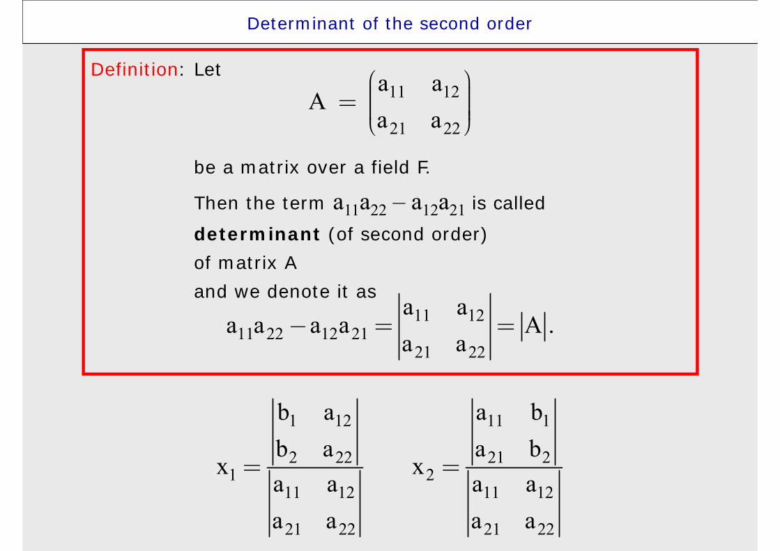
Definition: Let

be a matrix over a field F.

Then the term a11a22 – a12a21 is calleddeterminant (of second order) of matrix Aand we denote it as

Determinant of the second order

11 12

21 22

a aA

a aæ ö÷ç= ÷ç ÷ç ÷è ø

11 1211 22 12 21

21 22

a aa a a a A .

a a- = =

1 12 11 1

2 22 21 21 2

11 12 11 12

21 22 21 22

b a a bb a a b

x xa a a aa a a a

= =

a11x1 + a12x2 + a13x3 = b1a21x1 + a22x2 + a23x3 = b2a31x1 + a32x2 + a33x3 = b3

Lets multiply the first equation by a22a33 – a23a32,

the second equation by a13a32 – a12a33,

the third equation by a12a23 – a13a22,and then sum-up the first two with the third one and we get:

( a11a22a33 – a11a23a32 + a13a21a32

– a12a21a33 + a12a23a31 – a13a22a31 ) x1

= b1a22a33 – b1a23a32 + b2a13a32

– b2a12a33 + b3a12a23 – b3a13a22

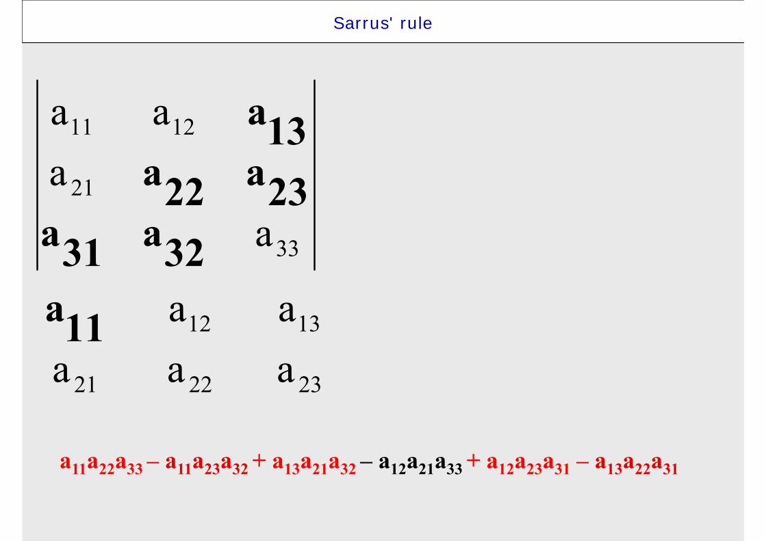
Determinant of the third order

Definition: Let A is a square matrix of the order of 3with the elements from the field F. Then the determinant (of the third order) of matrix A is the term

a11a22a33 – a11a23a32 + a13a21a32

– a12a21a33 + a12a23a31 – a13a22a31 =


11 12 13

21 22 23

31 32 33

a a aa a a A .a a a

= =

1 12 13 11 1 13 11 12 1

1 2 22 23 2 21 2 23 3 21 22 2

3 32 33 31 3 33 31 32 3

b a a a b a a a bA b a a , A a b a , A a a b ,

b a a a b a a a b

æ ö æ ö æ ö÷ ÷ ÷ç ç ç÷ ÷ ÷ç ç ç÷ ÷ ÷ç ç ç= = =÷ ÷ ÷ç ç ç÷ ÷ ÷ç ç ç÷ ÷ ÷ç ç ç÷ ÷ ÷÷ ÷ ÷ç ç çè ø è ø è ø

If we denote


31 21 2 3

AA Ax , x , x .

A A A= = =

then

Cramer’s rule

232221

131211

333231

232221

131211

aaaaaa

aaaaaaaaa

a11a22a33 – a11a23a32 + a13a21a32 – a12a21a33 + a12a23a31 – a13a22a31

Sarrus' rule

aaaaaa

aaaaaa

232221

131211

3231

2321

1312

33a22a

11a


Sarrus' rule

aaa

aa

aaaa

232221

1211

31

23

1312

13a33a32a

22a21a11a


Sarrus' rule

aa

a

aaa

2221

11

23

1312

23a13a12a33a32a31a

22a21a11a


Sarrus' rule

232221

131211

333231

232221

131211

aaaaaa

aaaaaaaaa


Sarrus' rule

31a22a

13a

232221

131211

3332

2321

1211

aaaaaa

aaaa

aa


Sarrus' rule

11a32a31a

23a22a13a

232221

1312

33

21

1211

aaaaa

aa

aa


Sarrus' rule

21a

12a11a33a32a31a23a22a13a

2322

13

21

1211

aaa

aaa


Sarrus' rule

Determinant of a square matrix

If is a square matrix of type , then the determinant is the exactly defined number

we denote as .

The minor is defined to be the determinant of the matrix that results from by removing

the th row and the th column.

The determinant itself is recursively defined as follows: If , then the determinant of matrix of type

is simply . If , then for each row index it holds:

This is called

the Laplace expansion along the ith row.

( ) ( ) ( )1 21 1 2 21 1 1 .i i i n

i i i i in ina a a+ + += - + - + + -A A A A

ija A n n

A

ijA 1 1n n A

i j

1n 11aA 1 1

11aA2n i

Determinant of a square matrix

If we have a LU decomposition of matrix A,then

where

= ⋅A L U

The number of arithmetic operations of LU decomposition is of order of n3.

This is much less (in case of determinants of higher order)much less then n! operation

necessary to perform if we use Lapalce expansionfor calculation of determinant.

11 22 33... nnl l l l=L 11 22 33... nnu u u u=U

Lecture 4

OUTLINE


Motivation

Many practical problemsrequire to solve

the large systems of linear equationsA x = b ,

in which the matrix A is sparse,i.e. it has relatively small number of nonzero elements.

Standard elimination methods are not suitable

for solving such large sparse linear systems.

( Why ? )

Because during the elimination process we fill-up positions of originally zero elements –

matrix is no more sparse.

Iterative methods

We chose an initial vector x0 andwe generate a sequence of vectors

which converge to the seeking solution x.0 1 2 , x x x

Common feature of all iterative methods is fact,that each iteration step

requires as many operations asmultiplication of matrix A by a vector,

which is for sparse matrices relatively small number of operations.

1k k+x x

Lecture 4

OUTLINE


Convergence

The most of classical iterative methodsare based on decomposition of matrix A = M – N,

where M is regular matrix.

1 ,k k+ = +Mx Nx bThen we can define a sequence of xk as

where initial approximation x0 is prescribed.

We say, that the iterative method converge,and we write ,

if numeral sequencek x x

0.k - x x

We denote the error of k th iteration.Because , we get

or

k k= -e x x

( ) ( )1k k+ - = -M x x N x x

= +Mx Nx b1

1 .k k-

+ =e M Ne

1 ,<T1-=T M N

Convergence of iterative methodis assured for any initial vector

if

where is iteration matrix.

Convergence

If we denote then we get

2 11 1 0 .k

k k k+

+ -£ ⋅ £ ⋅ £ £ ⋅e T e T e T e

1-=T M N

T is an arbitrary matrix norm

Recall – matrix norms

“Entrywise” norm of matrix

2

1 1

n n

ijFi j

aA= =

= åå Frobenius norm (consistent with l2)

( )

1

1 1

n n ppijp p

j jvec a

= =

æ ö÷ç ÷ç= = ÷ç ÷ç ÷è øååA A

,max iji j

a¥

=A max norm

Conditions for stopping iterations

How to decide, whether xk+1 is good enough approximation

of solution x ?

Usually we test one of the conditions:

1.

2.

1k k k+ - £x x x

( )1 1k k+ +£ ⋅ +r A x b

Lecture 4

OUTLINE


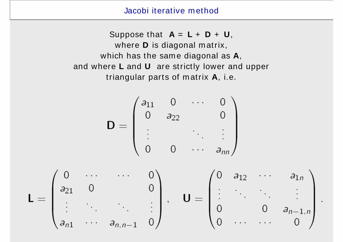
Jacobi iterative method

Suppose that A = L + D + U, where D is diagonal matrix,

which has the same diagonal as A,and where L and U are strictly lower and upper

triangular parts of matrix A, i.e.

Jacobi iterative method

Jacobi method is based on decomposition

A = M – N,where M = D and N = -(L+U)

and we write it as

( )1k k+ = - +Dx b L U x

This system is easy to solve.If we write it in component form then

( ) ( )1

1

1 , 1,2,..., .n

k ki i ij j

ii jj i

x b a x i na

+

=¹

æ ö÷ç ÷ç ÷ç ÷= - =ç ÷ç ÷ç ÷ç ÷÷çè ø

å

Analysis of propertiesof iteration matrix leads to the statement, that

Jacobi method converge, if A is diagonally dominant.

( )1-=- +T D L U

Recall

Definition: We say that square matrix Ais diagonally dominant if

Lecture 4

OUTLINE


Gauss-Seidel method

Recall the Jacobi method

( ) ( )1

1

1 , 1,2,..., .n

k ki i ij j

ii jj i

x b a x i na

+

=¹

æ ö÷ç ÷ç ÷ç ÷= - =ç ÷ç ÷ç ÷ç ÷÷çè ø

å

If we use instead of

we get

Gauss-Seidel method

( )kix( )1k

ix +

( ) ( ) ( )1

1 1

1 1

1 , 1,2,..., .i n

k k ki i ij j ij j

ii j j ix b a x a x i n

a

-+ +

= = +

æ ö÷ç ÷ç= - - =÷ç ÷ç ÷è øå å

Gauss-Seidel method

In a matrix form

( ) 1k k++ = -D L x b Ux

( )1k k+ = - +Dx b L U x

For comparison, the Jacobi method in matrix form reads

Analysis of propertiesof iteration matrix leads to the statement, that

Gauss-Seidel method converge, if A is diagonally dominant

orpositive-definite.

( ) 1-=- +T D L U

Definition: Symmetric matrix A is positive-definite if

for any non-zero vector x it holds

0Tx x⋅ ⋅ >A

Gauss-Seidel method

Checking, whether the matrix is positive-definiteis usually problematic.

If we multiply any regular matrix A from left bytheir transpose matrix,

the final matrix

is symmetric and positive-definite.

Therefore, for system

it is assured that Gauss-Seidel method converge.

In such a case the convergence could be very slow.

TA A

T T=A Ax A b

Jacobi method vs Gauss-Seidel method

• Convergence of Gauss-Seidel methodis usually faster thenconvergence of Jacobi method

• There are matrices, for which the Gauss-Seidel method convergebut Jacobi notand vice versa

• Jacobi method allows parallel processing,while the Gauss-Seidel methodis sequential from their core

Summary

• Gauss elimination method and Cramer’s rulelead to the solution.(Without round off errors we could findthe exact solution.)

• The base of GEM is the modification of matrixto triangular form. (using elementary row operations)

• The influence of round-off errors on GEM could be considerable, therefore we use partial pivoting.

• The GEM is demanding from time and memory aspects. It is best suited for not very large systems with dense matrix.

• The Cramer’s rule is suitable only for very small systems.

Summary

• Using the iterative method we usually find only approximate solution.

• At the beginning we chose the initial approximation of solution and we refine the solution by repeatedly inserting it into iteration formula.The computation is usually finished when the norm of difference of two consecutive iterations is small enough.

• Iterative methods could also diverge.This depend on the properties of the matrix.

• Iterative methods are suitable for solving large systems with sparse matrix.

Lecture 4

OUTLINE


Stationary iterative methods

Jacobi and Gauss-Seidel methods are so calledstationary iterative methods.

Stationary iterative methods solve a linear system with an operator

approximating the original one; and based on a measurement of the error in the result,

form a "correction equation" for which this process is repeated.

While these methods are simple to derive, implement, and analyze,

convergence is only guaranteed for a limited class of matrices.

Linear stationary iterative methods are also called relaxation methods.

Krylov subspace methods

Krylov subspace methods work by forming a basis of the sequence

of successive matrix powers times the initial residual (the Krylov sequence).

The approximations to the solution are then formed by minimizing the residual over the subspace formed.

The prototypical method in this class is the conjugate gradient method (CG).

Lecture 4

OUTLINE

1. Determinants and Cramer’s rule2. Iterative method for solving linear systems3. Convergence, iteration matrix, stop criteria4. Jacobi method, Gauss-Seidel method5. Krylov subspace methods

• Conjugate gradient method• Generalizations of CG method• Convergence of CG method

6. Preconditioning7. Singular value decomposition

Conjugate gradient method (CG)

The conjugate gradient method is implemented as an iterative algorithm,

applicable to large sparse systemswith

symmetric, positive-definite matrix.

We say that two non-zero vectors u and v are conjugate (with respect to A) if

0Tu Av


The iterative algorithms is described by this formulas:

( ) ( ) ( )

( ) ( )

( ) ( )

( ) ( ) ( )

( ) ( ) ( )

( ) ( )

( ) ( )

( ) ( ) ( )

1 1 1

1

1

1

1 1

,

,

,

,

,

.

k T k

k k T k

k k kk

k k kk

k T k

k k T k

k k kk

+

+

+

+ +

= = -

=

= +

= -

=-

= +

v r b Ax

v r

v Av

x x v

r r Av

v Ar

v Av

v r v


From the fundamentals of algorithm it followsthat after n iterations

we obtain exact solution of the systemand therefore it is not an iterative method

in a strict sense.

This would be true only if there areno round-off errors.

Therefore we have to look at CG method as an iterative method

and we have to define stop criteria.

Lecture 4

OUTLINE




Generalizations of CG method

In case of nonsymmetrical andnot necessary positive-definite matrices

we usebiconjugate gradient method

(e.g. subroutine linbcg from Numerical Recipes).

The ordinary conjugate gradient methodis their special case.

Generalizations of CG method

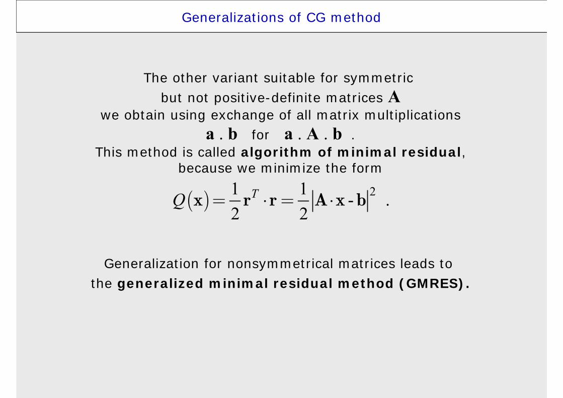
The other variant suitable for symmetric but not positive-definite matrices A

we obtain using exchange of all matrix multiplicationsa . b for a . A . b .

This method is called algorithm of minimal residual,because we minimize the form

Generalization for nonsymmetrical matrices leads to the generalized minimal residual method (GMRES).

( ) 21 1 - .2 2

TQ = ⋅ = ⋅x r r A x b

Lecture 4

OUTLINE




Convergence of CG method

Let x(k) be an approximate solution in the k-th step of CGand let x* be the exact solution.

For symmetric, positive-definite matrix we definecondition number of matrix κ(A)

and A-norm of an arbitrary vector z :

( )( )( )

( )1/ 2max

min: , : , .

= =A

AA z Az z

A

Then

If κ(A) >> 1 the convergence is very slow.

( ) ( )( )

( )112

1

k

k

é ù-ê ú- £ -ê ú+ê úë û

A A

Ax* x x* x

A

Lecture 4

OUTLINE


Preconditioning

The aim of preconditioning isto speed-up the convergence of iterative method in such a way,

that we solve an alternative system of linear equationsin which the coefficient matrix has

lower condition number κthen the original coefficient matrix.

Let A.x = b be the original linear system.

Left preconditioning is defined as:Let matrix M is regular and „close“ to matrix A.

Then we solve the system

Right preconditioning is defined as:Let matrix M is regular. Then we solve system

-1 -1=M Ax M b

-1 1, .-= =AM u b x M u

Preconditioning in CG method

Original algorithms CG:

( ) ( )

( ) ( )

( ) ( )

( ) ( )

( ) ( ) ( )

( ) ( ) ( )

( ) ( )

( ) ( )

( ) ( ) ( )

1 1

1 1

1

1

1

1 1

k T k

k k T k

k k kk

k k kk

k T k

k k T k

k k kk

+

+

+

+ +

= -

=

=

= +

= -

=-

= +

r b Ax

v r

v r

v Av

x x v

r r Av

v Ar

v Av

v r v

( ) ( ) ( ) ( )

( ) ( )

( ) ( )

( ) ( )

( ) ( ) ( )

( ) ( ) ( ) ( ) ( )

( ) ( )

( ) ( )

( ) ( ) ( )

1 11

1

1 11

1 1

1 1

1

1

1

1 1

,

, k k

k T k

k

k T k

k k T k

k

T

k kk

k k kk

k

k k

k

kk

+

-

+ +

+ +

-

+

+

+

= -

=

=

= +

= -

=

=

= +

=

z M r

z

z

z M r

z r

z

r b Ax

v

r

v Av

x x v

r r Av

zv v

r

Algorithm of preconditioned CG:

Jacobi preconditioner

One of the simplest forms of preconditioning, is obtained by the choosing the preconditioner

to be the diagonal of the matrix matice A

Then

This preconditioning we callJacobi preconditioner

ordiagonal scaling.

Advantages of Jacobi preconditioner arethe easy implementation andlow memory requirements.

{if

0 ifii

ijA i j

Mi j

==

¹

1 .ijij

iiM

A- =

Other types of preconditioning

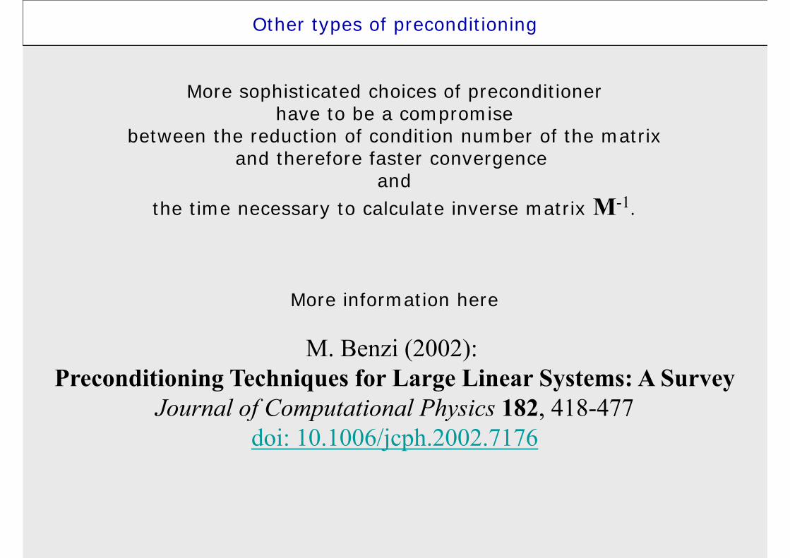
More sophisticated choices of preconditionerhave to be a compromise

between the reduction of condition number of the matrixand therefore faster convergence

andthe time necessary to calculate inverse matrix M-1.

More information here

M. Benzi (2002):Preconditioning Techniques for Large Linear Systems: A Survey

Journal of Computational Physics 182, 418-477doi: 10.1006/jcph.2002.7176

Example

Example

Lecture 4

OUTLINE


• Introduction• SVD of a square matrix• SVD for less equations than unknowns• SVD for more equations than unknowns

Lets have a square matrix A.

Its eigenvalues will be denoted as λn ,

right and left eigenvectors as x and y ,and it holds

If and is symmetric,then λi, xi ≡ yi and

eigenvectors generate the orthogonal base.

Affine transform P-1APdoes not change the eigenvalues of matrix A.

Terminology and basic relations

( )det 0

i i iT Ti i i

- =

=

=

A I

Ax x

y A y

ÎÂAÎÂ

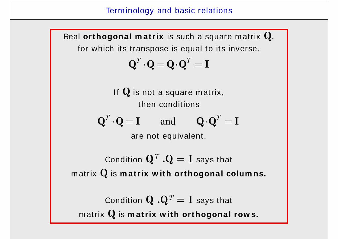
Terminology and basic relations

Real orthogonal matrix is such a square matrix Q,for which its transpose is equal to its inverse.

If Q is not a square matrix,then conditions

are not equivalent.

Condition QT .Q = I says that

matrix Q is matrix with orthogonal columns.

Condition Q .QT = I says that

matrix Q is matrix with orthogonal rows.

T T⋅ = ⋅ =Q Q Q Q I

andT T⋅ = ⋅ =Q Q I Q Q I

If the number of equations M is less than the number of unknowns N,or if M = N but equations are linearly dependent,

then the system has no solutionor

it has more than one solution.

In the later case the space of solutions is given bya particular solution

added to the any linear combination of N - M vectors.

The task to find the space of solution for matrix Ais possible to solve using

singular value decomposition of matrix A.

Singular value decomposition - introduction

If the number of equations M is greater than the number of unknowns N,then in general there is no solution vector and

the system is called overdetermined.

However, we could find a best “compromise” solution, which is “the closest” solution

that satisfy all equations.

If „the closest“ we define in a sense of least square,i.e. the sum of square of residuals is the smallest possible,

then the overdetermined system is reduced tosolvable problem

called the least square method.


Reduced system of equations could be written assystem N x N equation

This equations we call normal equationsof a least square problem.

Singular value decomposition has many common featureswith the least square method,

which we show later.

Direct solution of normal equations is in generalnot the best way to find a solution of least square problem.


( ) ( ) .T T⋅ ⋅ = ⋅A A x A b

Singular value decomposition

In many cases,when GEM or LU decomposition fail,

singular value decomposition (SVD)precisely diagnose, where is the problem

and in many cases it also offer a suitable numerical solution.

SVD is also methodto solve many least square problems.


SVD is based on the following theorem of linear algebra:

Each matrix A of type M x N,

which the number of rows M is greater or equal to the number of columns N,could be decomposed to a product of

matrix with orthogonal columns U of type M x N,

diagonal matrix W of type N x Nwith positive or zero entries (singular values)

and transpose orthogonal matrix V of type N x N.


Orthogonality of matrices U and V could be written as


SVD could be done also if M < N.

In such a case the singular values wj for j = M+1, …, Nare all zero

as well as corresponding columns of matrix U.

There is a lot of algorithms of SVD,proven is subroutine svdcmp from Numerical Recipes.

Lecture 4

OUTLINE



Singular value decomposition of a square matrix

If A is a square matrix of type N x N,

then U , W and V are all square matrices of type N x N.

Because U and V are orthogonal,their inverse are equal to transpose.

Then we can write a formula for inverse matrix A

( )1 diag 1/ Tjw- é ù= ⋅ ⋅ê úë ûA V U

SVD offers clear diagnosis of situation,if some of singular values are zero

or close to zero.


Recall one of definition ofcondition number of matrix κ(A):

The matrix is singular if its condition umber is infinity.

The matrix is ill-conditionedif reciprocal value of its condition number

is close to the machine epsilon of a computer,i.e. less than 10-6 for single precision or

10-12 for double precision.

( ){ }{ }

1 max:

minj

j

w

w A A A-= =


The case of system

in which the coefficient matrix A is singular:

At first, lets have a look at the homogeneous case,i.e. the case of b=0.

In other wordswe are looking for null space of A

,⋅ =A x b

( ) { } { }{ } { }

: :

: :

n n T

n T T n T

null A x Ax 0 x UwV x 0

x U UwV x 0 x wV x 0

= Î = = Î =

= Î = = Î =


The case of system


At first, lets have a look at the homogeneous case,i.e. the case of b=0.

In other wordswe are looking for null space of A

SVD gives direct solution – each column of matrix V,

which corresponding singular value wj is zerois a solution.

,⋅ =A x b


The case of system


Now lets have a look at range of matrix A

,⋅ =A x b

( ) { } { } { }: : :n T n n

T

range A Ax x UwV x x Uwy y

y V x

= Î = Î = Î

=


The case of system


Now lets have a look at range of matrix A

,⋅ =A x b

The range of matrix A is composed by spanof columns of matrix U,

which corresponding singular value wj is nonzero.


The solution of a system with nonzero right-hand-sideusing SVD is this:

• we exchange 1/wj by zero if wj=0• then we calculate (from right to left)

( ) ( )diag 1/ Tjwé ù= ⋅ ⋅ ⋅ê úë ûx V U b

If a particular solution lies in range of A,

then it has the smallest size .2x

If a particular solution does not lies in range of A,

then x minimize the residuum of solution .:r = ⋅ -A x b


Matrix A is not singular


Matrix A is singular


Up till now we considered only extreme casesthat the coefficient matrix is or is not singular.

There is often the casethat the singular values wj are very small but nonzero,

so the matrix is ill-conditioned.

In such a case direct methodscan offer formally the solution,

but the solution vector has unreasonably large entries,which during the algebraic manipulations with matrix A

leads to very bad approximation of the right-hand-side vector.

At that time is better small values wj set to zero andthe solution calculate using

(with replace of 1/wj by zero if wj=0)( ) ( )diag 1/ T

jwé ù= ⋅ ⋅ ⋅ê úë ûx V U b

We have to be cautious andwe have to chose the good threshold level for zeroise of wj

Lecture 4

OUTLINE



Singular value decomposition for less equations than unknowns

If we have less equation than unknownswe expect N - M dimensional space of solutions.

In this case SVD offersN - M zero or negligible small values of wj.

If some of M equations degenerate,then we could have additional zero-valued wj .

Then those columns of V,

which corresponds to zero singular value wjmakes a basis vectors of seeking solution space.

Particular solution could by find using

( ) ( )diag 1/ Tjwé ù= ⋅ ⋅ ⋅ê úë ûx V U b

Lecture 4

OUTLINE



Singular value decomposition for more equations than unknowns

If we have more equations than unknownswe are seeking solutionin a least square sense.

We are solving system written as:

Singular value decomposition for more equations than unknowns

After SVD of matrix A we have

the solution in a form

In this case usually it is not necessary set to zero values wjhowever the unusually small values indicate

that the data are not sensitive to some parameters.

Lecture 4

OUTLINE


• Conjugate gradient method • Generalizations of CG method • Convergence of CG method



Date post:	21-Oct-2019
Category:	Documents
Upload:	others
View:	12 times
Download:	0 times

Numerical methods - fyzikazeme.sk · iiijj ii j ji xbax i n a + = ¹ æö çç ÷÷ =- =çç ÷÷...

Documents