20
| Date post: | 04-Apr-2018 |
| Category: |
Documents |
| Upload: | duongkhanh |
| View: | 215 times |
| Download: | 2 times |

Scientia Iranica, Vol. 15, No. 5, pp 516{535c Sharif University of Technology, October 2008
Numerical Modeling of HydraulicFracturing in Oil Sands
A. Pak1;� and D.H. Chan2
Hydraulic fracturing is a widely used and e�cient technique for enhancing oil extraction fromheavy oil sands deposits. Application of this technique has been extended from cemented rocksto uncemented materials, such as oil sands. Models, which have originally been developedfor analyzing hydraulic fracturing in rocks, are in general not satisfactory for oil sands. Thisis due to a high leak-o� in oil sands, which causes the mechanism of hydraulic fracturing tobe di�erent from that for rocks. A thermal hydro-mechanical fracture �nite element model isdeveloped, which is able to simulate hydraulic fracturing under isothermal and non-isothermalconditions. Plane strain or axisymmetric hydraulic fracture problems can be simulated by thismodel and various boundary conditions, such as speci�ed pore pressure/ uid ux, speci�edtemperature/heat ux, and speci�ed loads/traction, can be modeled. The developed model hasbeen veri�ed by comparing its results to existing analytical and numerical solutions for thermo-elastic consolidation problems. The model has been used to simulate a laboratory experimentof hydraulic fracture propagation in oil sands. The results from the numerical model are inagreement with experimental observations. The numerical model and laboratory experimentsboth indicate that, for uncemented porous materials, such as sands (as opposed to rocks), asingle planar fracture is unlikely to occur and a system of multiple fractures or a fracture zoneconsisting of interconnected tiny cracks should be expected.
INTRODUCTION
Hydraulic fracturing is a widely used technique toenhance oil and gas production. The technique wasintroduced to the petroleum industry in 1947, and isnow a standard operating procedure. By 1981, morethan 800,000 hydro fracturing treatments had beenperformed and recorded. Today, about 35% to 40% ofall currently drilled wells are hydraulically fractured [1].
Since its inception, hydraulic fracturing has devel-oped from a simple low volume and low injection ratereservoir stimulation technique to a highly engineeredand complex procedure that can be used for many pur-poses. Figure 1 depicts a typical hydraulic fracturingprocess in the petroleum industry. The procedure isas follows. First, a neat uid, such as water (called
1. Department of Civil Engineering, Sharif University ofTechnology, Tehran, Iran.
2. Department of Civil and Environmental Engineering,University of Alberta, 3-133 NREF Building, T6G 2W2,Edmonton, Al1berta, Canada.
*. To whom correspondence should be addressed. E-mail:[email protected].
Figure 1. Typical hydraulic fracturing treatment inpetroleum industry (after [1]).
`pad'), is pumped into the well at the desired depth(pay zone), to initiate the fracture and to establishits propagation. This is followed by pumping slurry,which is a uid mixed with a propping agent, such assand (often called a `proppant'). This slurry continuesto extend the fracture and concurrently carries theproppant deeply into the fracture. After pumping,the injected uid chemically breaks down to a lowerviscosity and ows back out of the well, leaving a highlyconductive propped fracture for oil and/or gas to easily

Numerical Modeling of Hydraulic Fracturing in Oil Sands 517
ow from the extremities of the formation into thewell. It is generally assumed that the induced fracturehas two wings, which extend in opposite directionsfrom the well and is oriented, more or less, in avertical plane. Other fracture con�gurations, such ashorizontal fractures, are also reported to occur, butthey constitute a relatively low percentage of situationsdocumented. Experience indicates that at a depthof below 600 meters, fractures are usually orientedvertically. At shallow depths, horizontal fractures havebeen reported [1]. The fracture pattern, however, maynot be the same for di�erent types of soil and rock.
`Oil sands' exist in some parts of the world asthick deposits in deep and semi-deep undergroundlayers. For extraction of oil from oil sand deposits,one of the widely used methods, as described above, ishydrofracturing, in which hot water/steam is injectedinto the wells at a very high rate and temperature.Although sand is a cohesionless material, the viscousbitumen that exists in the porous medium causes thecombination of sand and bitumen to behave like aporous rock that may experience fracturing due to highinjection pressure. The study of types and patterns offracture in uncemented oil sand deposits, by means ofnumerical modeling, is the basic objective of this paper.
For decades, petroleum engineers have been de-veloping models for simulating hydraulic fracturing inoil reservoirs. In the early 1960's, the industry felt theneed for a design tool for this fast growing technique.In response to this need, a number of two-dimensional(2-D) models were developed for designing hydraulicfracturing treatments. This type of simple closed formsolution has been used by the industry with somesuccess; however, as the technology progressed fromlow volume/rate to high volume/rate treatments inmore sophisticated and massive hydraulic fracturingprojects, the industry demanded more rigorous designmethods in order to minimize costs. In the last 20years, a number of 2-D and 3-D numerical modelshave been developed (some of these models will bediscussed later). The most common equations usedin these numerical models are uid ow and heattransfer equations, which are usually solved iteratively.Geomechanical aspects are incorporated in some ofthe models, mostly in an uncoupled manner. Mainlyvertical or horizontal planar fractures were considered,based on the 2-D closed form solutions mentionedabove. The degree of sophistication of these modelsvaries considerably and their results cannot be vali-dated with much con�dence. The main problem invalidating these models is that the con�guration ofthe induced fracture is not really known; therefore, theresults of the model are usually evaluated based on uidinjection pressure measurements and/or the productionhistory of the well.
The application of these models to oil sands,
however, has not been very successful and predictionsof the model, in some cases, have been poor. Someresearchers attribute the discrepancy to the e�ect ofhigh leak-o� rates in oil sands. On the other hand, thepeculiar characteristics of oil sand, such as an inter-locked structure with a high dilation rate, a nonlinearstress-strain behavior with strain softening after thepeak, a dilation phenomenon at shear failure and atemperature-dependent behavior, may also contributeto the discrepancy between model predictions and �eldmeasurements.
In this paper, a brief overview of the earlier stud-ies will be presented and a mathematical formulation ofthe developed fully coupled thermal hydro-mechanicalfracture model will be discussed in detail. Modeling ofthe fracture process and its numerical treatment willthen be explained and benchmarking of the developed�nite element model will be presented by comparingits results to the existing analytical, numerical andexperimental solutions.
EARLIER STUDIES OF HYDRAULICFRACTURING
Zheltov and Khristianovitch [2], Perkins and Kern [3]and Geertsma and Deklerk [4] are among the �rstinvestigators to develop models for hydraulic frac-turing. Zheltov and Khristianovitch [2] introducedthe concept of mobile equilibrium, i.e. slow movingfracture propagation as a result of hydraulic action.Geertsma and Deklerk [4] used their concepts andprovided a closed form solution for a planar fracture.This model is based on the assumption of plane straindeformation in a `horizontal plane' and is usually calledthe GdK model. Perkins and Kern [3] proposed adi�erent closed form solution for hydraulic fracturepropagation problems. The model is based on theassumption of plane strain deformation in a `verticalplane'. Nordgren [5] improved this work by incorpo-rating the e�ect of leak-o� and, hence, this model isusually called PKN. In these models, the height ofthe fracture, hf , is considered to be known, which isequal to the thickness of the oil-bearing layer (pay).For the determination of other values, such as fracturelength (Lf ), maximum fracture opening and injectionpressure, a set of equations has been derived.
There have been some e�orts to simulate 3-D frac-ture propagation [6,7]. In these models, the assumptionof isotropic elasticity is used and the e�ects of porepressure are neglected. The elasticity equations arecoupled with the equation of ow inside the fractures.In these models, the concept of inducing a planarfracture is retained but the height of the fracture isnot �xed and varies with changes in stress. Fractureextension is controlled by a linear elastic fracturemechanics criterion. Advani et al. [8] developed a �nite

518 A. Pak and D.H. Chan
element program for modeling 3-D hydraulic fracturesin multi-layered reservoirs. They extended the earlierwork of the Pseudo three-dimensional (P3D) modelpresented by Advani and Lee [9] and other investigatorsin the early 80's. This work investigated tensile planarhydraulic fracture propagation in layered reservoirswith elastic behavior.
Settari and Raisbeck [10,11] provided two of theearly work on hydraulic fracture simulation in `oil sanddeposits'. In 1979, they developed a two dimensional�nite di�erence model for single-phase compressible uid ow in a linear elastic porous material with atensile fracture, similar to the PKN model. This modelwas extended to a two-phase thermal ow [11] in orderto describe the process of a �rst cycle steam injectionfor three di�erent fracture geometries.
Atukorala [12] developed a �nite element modelfor simulating either horizontal or vertical hydraulicfracturing in oil sands. In this work, for the sakeof simplicity, the uid ow analysis was separatedfrom stress analysis. These two equations were solvediteratively by imposing a compatibility condition onthe volume of the uid in the fracture. The fractureshape was assumed elliptic with blunt tips, in orderto avoid the singularity of stresses at the crack tip.A linear elastic fracture mechanics criterion was usedfor analyzing the tensile fracture in a nonlinear elasticdomain. No thermal e�ect was considered in this study.
Settari et al. [13] investigated the e�ects of soildeformation and fracture on the reservoir in a partiallycoupled manner. The e�ect of leak-o� on fracturedimensions was emphasized. Oil sand failure wasconsidered to be shear failure with a Mohr-Coulombcriterion. Dilation was not modeled in this work, butit was assumed that a constant change in volumetricstrain occurs after reaching a peak shear stress (fail-ure). They developed a computer program, calledCONS, based on the above, partially coupled stress- ow, analysis. Settari [14,15] extended this work byincorporating temperature e�ects (thermal ow) in theformulation.
Frydman and Fontoura [16] simulated the processof borehole pressurization, the mechanism for whichis the same as hydraulic fracture treatment with acoupled hydromechanical approach. They developeda new fracture element, considering the e�ect of acohesive zone in crack analysis. In their work, thedirection of the fracture propagation was prede�nedand no thermal e�ect was considered.
Ouyang et al. [17] developed a mathematicalmodel and employed an adaptive �nite element schemeto simulate the distribution of proppant in a propagat-ing hydraulic fracture.
Itaoka et al. [18] studied the crack growth behav-ior under high tectonic stress, conditions correspondingto great depths. Their study presents a �nite element
model for the analysis of hydraulic fracturing, takinginto account the mixed-mode fracture. They inves-tigated crack growth behavior as the mode of crackpropagation.
Yang et al. [19] numerically studied the e�ect ofheterogeneity and permeability on the initiation andpropagation of hydraulic fracturing.
Reynolds et al. [20] used Stimplan software pack-age to determine the optimum fracture dimensions,sizing and sand schedule. Stimplan is a pseudo 3-D, nu-merical model performing an implicit �nite di�erencesolution to basic equations of mass balance, elasticityand uid ow.
Lu et al. [21] developed a pseudo 3-D hydraulicfracturing using radial ow, which made a betterprediction regarding fracture height.
Cook et al. [22] conducted a joint experimental-numerical study regarding the exploration of near-well bore mechanics. An experimental procedure,using a true-triaxial apparatus, was developed for thelaboratory simulation of slurry injection, and a DiscreteElement Method (DEM) numerical model was used forsimulation of the experiments. They found that, underisotropic horizontal stress conditions, multiple verticalfractures were induced and propagated in randomorientations.
In the early models, it was assumed that fracturein oil sand is similar to fracture in soft cementedrock, such as sandstone; however, the prediction ofthese models did not match �eld observations. Forexample, the fracture length was smaller than thevalue predicted by the models, the fracture openingwas larger and the injectivity was much higher thananticipated. These facts indicated that hydraulicfracturing in oil sand, contrary to rock, is dominatedby leak-o�. This high leak-o� cannot be adequatelydescribed by classical models, such as those proposedby Carter [23] or Nordgren [5]. In order to describe thissituation, geomechanical aspects have to be invoked.By incorporating the geomechanical behavior of oilsand in the model, such as shear failure and dilatione�ects (and the corresponding increase in porosityand permeability), a signi�cant improvement in theresults of the model was observed. From a reservoirengineering viewpoint, the main objective of modelingis being able to predict the production rates of oilwells. Thus, geomechanical aspects are employed inthese models, mainly to better improve their predictionability.
Fracture modeling in porous materials is clearlydependent on the stress �eld in the soil, as well as pore uid pressures. Therefore, contrary to most availablereservoir engineering models, any attempt to simulatehydraulic fracturing in oil sand deposits should incor-porate a detailed stress/deformation analysis.
It should be noted that, in hydraulic fracturing,

Numerical Modeling of Hydraulic Fracturing in Oil Sands 519
four processes are acting simultaneously. Grounddeformation, uid ow, heat transfer, and fracturingphenomenon are the main issues involved in hydraulicfracturing. Therefore, for the modeling of hydraulicfracturing in geomaterials, at least three conservationlaws for applied load, uid ow, and heat transfer, inthe form of three partial di�erential equations, haveto be solved simultaneously. Fracture con�gurationshould be based on stress/deformation analysis in theground. In this case, imposing a kind of prescribedfracture geometry on the model is not necessary.
FORMULATION OF THE FULLYCOUPLED THERMALHYDROMECHANICAL (THM) MODEL
In formulating the model, three partial di�erentialequations of equilibrium, continuity of uid ow, andheat transfer are considered in incremental forms.Changes in displacement in three directions, f�Ug,changes in pore pressure �P , and changes in tem-perature �T , are the primary unknowns, which de�nethe state of any point inside the domain. Since smallstrains/displacements are assumed, f�Ug, �P and�T , during a time increment, `�t', are small and sec-ond (or higher) order incremental terms are neglectedin the formulation. In this section, a superimposed dotmeans a derivative with respect to time, `*' stands fornodal values and `-' means prescribed values. Subscript`t' means the value at time t, and subscript `,' indicatesa derivative with respect to the coordinate axes.
An equilibrium equation is used as the basis forthe deformation analysis. The equilibrium equation inan incremental form reads as follows [24,25]:
��ij;j + �Fi = m0� �Ui + C 0� _Ui: (1)
A weighted residual method is used for obtaining theweak form of Equation 1. After integration by parts:ZS
��ijnj!ds�ZV
��ij!;jdV
=ZV
(��Fi +m0�Ui + c0�Ui)!dV;(2)
the following boundary conditions are considered (Fig-ure 2):
- Stress boundary condition (natural B.C.):
��ijnj = �tsi on S�; (3)
- geometric boundary condition (essential B.C.):
Ui = U i on Su: (4)
Figure 2. Boundary conditions of a typical domain.
Since dynamic e�ects are not considered in this study,inertia and damping terms will be neglected. The prin-ciple of e�ective stress can be written in an expandedform incorporating the e�ect of thermal expansion:
��ij = ��0ij ��P�ij
= Dijkl
��"kl � 1
3�s�kl�T
���P�ij : (5)
For consistency with the other two conservation laws,`P ' is considered to be positive in compression.Soil/rock particles are considered to be incompress-ible and the e�ect of creep and/or other strains aredisregarded in Equation 5. Assumption of the in-compressibility of solid grains is usually valid, sincethe compressibility of pore uid, especially pore uidwith occluded gas bubbles, such as oil (bitumen), isvery high. Thus, in comparison, the compressibilityof solid grains can be neglected. Equation 5 can beused for substituting total stress with e�ective stressin Equation 2.
In order to obtain the �nite element form ofEquation 2, spatial discretization can be performed,using the following relationships:
�Ui = [N ]f�U�g; �"ij = [B]f�U�g;�"V = [C]f�U�g;�P =< NP > f�P �g; �P;j = [BP ]f�P �g;�T =< NT > f�T �g; �T;j = [BT ]f�T �g: (6)
By employing the Galerkin method:
[!] = [N ] and [!];j = [B]; (7)
`N ' indicates the shape function matrix and `B' isthe derivative of shape functions, with respect to thespatial coordinates x, y and z. In order to makeit possible to use di�erent interpolation schemes forcalculating displacements, pore uid pressures, andtemperatures, di�erent `N ' and `B' will be used for
520 A. Pak and D.H. Chan
pore uid pressures and temperatures. These will bedesignated by subscripts `P ' and `T ', respectively. Forcalculating displacements, 8-node rectangular isopara-metric elements are used. For calculating pore pres-sures and temperatures, however, 8-node rectangularelements are changed to 4-node rectangular elementsby using the appropriate shape functions. It has beengenerally observed [26,27] that, in order to obtain com-patible coupled �elds, the displacement interpolationshould be one order higher than the pore pressureinterpolation. Also, Aboustit et al. [28] have reportedthat the use of a 4-node rectangular element for porepressures, along with an 8-node rectangular element fordisplacements, resulted in less oscillation in the analysisof a consolidation problem (compared to a case in whichan 8-node element was used for both pore pressure anddisplacements).
By substituting Equations 3 to 7 into Equation 2,the following equation is obtained:0@� Z
V
[B]T [D][B]dV
1A f�U�g+
0@ZV
[B]T fmg < NP > dV
1A f�P �g+
0@ZV
[B]T [D]13�Sfmg < NT > dV
1A f�T �g= �
ZS�
[N ]T f�tSgdS +Z
lim itsV [N ]T (�f�Fg
+m0f� �Ug+ c0f� _Ug)dV: (8)
In Equation 8, fmg represents the Kronecker deltain vector form. The �nal �nite element form of thisequation would be:
[K11]�U� + [K12]�P � + [K13]�T � = fF1g; (9)
where K11, K12 and K13 represent the factors of �U�,�P � and �T � in Equation 8, respectively, and thewhole right-hand side of this equation is shown as F1.
For uid ow, the mass continuity equation forporous media is used [29]:
r:(�v)�G = � @@t
(��): (10)
By applying the weighted residual method to obtainthe weak form of this equation and then integrating by
parts, Equation 10 becomes:ZS
(�v)ini!dS �ZV
(�v)i!;idV = �ZV
@@t
(��)!dV
+ZV
G!dV: (11)
Two types of boundary condition are considered asfollows (shown in Figure 2):
- Speci�ed velocity ( ux) at the boundary:
vi = vi on Sv; (12)
- Speci�ed pore uid pressure at the boundary:
P = P on Sp: (13)
The terms �, �, @�@t , @�@t and vi can be substituted withrelations described below, assuming that the rate ofchange, with respect to time, can be approximated bythe change during the time increment �t:
a) Porosity
�t =�VVVb
�t
=Vb � VSVb
; (14)
where Vb is the bulk volume of soil/rock and VVand Vs are the volume of voids and the volume ofsolids, respectively.
�t+�t =(Vb + �Vb)� (Vs + �Vs)
(Vb + �Vb): (15)
Now, �Vb = "V :Vb by de�nition and �Vs =Vs�S�T , assuming that the change in the volumeof solids can be mainly attributed to the thermalexpansion of solids, because the compressibility ofsolids compared to the compressibility of pore uidand bulk medium, is negligible. Hence, the volumechange of solids, due to change in pore pressureand e�ective stresses, can be ignored. Therefore,by substitution for �Vb and �Vs in Equation 15and some manipulations, one obtains:
�t+�t =1
1 + "V[�t + "V � �S�t(1� �t)]; (16)
and:
�� = �t+�t � �t =1� �t1 + "V
("V � �S�t); (17)
b) Fluid density: Variations of uid density withchanges in pressure and temperature can be de-scribed as follows:
�t = �0f[1 + �T (P � P0)][1� �P (T � T0)]g: (18)

Numerical Modeling of Hydraulic Fracturing in Oil Sands 521
Assuming that �P and �T are the coe�cients of uid thermal expansion and uid compressibility,respectively, Equation 18 can be written for time`t+ �t' in the following form:
�t+�t = �t(1 + �T�P )(1� �P�T ); (19)
�� = �t+�t � �t = �t�T�P � �t�P�T
��t�T�P�P�T ��t(�T�P � �P�T ); (20)
c) Fluid velocity: Darcy's law, in general index form,is given by:
vi = �Kij@H@xj
; (21)
where K is permeability (m/sec) and H is totalhead. Representing K in terms of absolute per-meability, k (m2), and expanding H yields thefollowing:
vi =� kij �
�z +
P
�;j
= �ki3�g�� kij
�@P@xj
+kijP ( @�@xj )
��; (22)
where �, z, P and are dynamic viscosity of uid, elevation, pore pressure and uid unit weight,respectively. The term ki3 represents the third rowof the permeability tensor corresponding to the zaxis.
By discretization in space, as described in Equation 6,the relationship for velocity can be expanded as follows:
vi =� ki3�tg�t
+kij [BP ]fP �t g
�t� kij�[BP ]f�P �g
�t
+kij < NP > fP �t g
�t�t@�t@xj
+kij� < NP > f�P �g
�t�t@�t@xj
: (23)
� is a number which may vary from 0 (explicit scheme)to 1.0 (implicit scheme). All values with the subscript`t' denote that they are considered to be at time `t'(known), for the sake of simplicity. They are modi�edat the end of each time step. Three terms, withoutthe primary unknown (�P �), are lumped together intoZi, which represents the velocity at time `t'. The tworemaining terms with (�P �) constitute �vi.
vi = �Zi � ��kij [BP ]�t
� kij < NP >�t�t
@�t@xj
�f�P �g;
(24)
where:
Zi =ki3�tg�t
+kij [BP ]fP �t g
�t
� kij < NP > fP �t g�t�t
@�t@xj
: (25)
In summary, the following relations are used in theformulation:� = (1� �)�t + ��t+�t = �t + ���
= �t + ��
1� �t1 + "v
("v � �S�T )�; (26)
� = (1� �)�t + ��t+�t = �t + ���
= �t + ��t(�T�P � �P�T ); (27)
@�@t� ��
�t=
1� �t1 + "V
("V � �S�T )�t
; (28)
@�@t� ��
�t=
�t�t
(�T�P � �p�T ); (29)
vi = (1� �)vit + �vit+�t = vit + ��vi
=
"kij �
�z +
P
�;j
#t
+��
"kij �
�z +
P
�;j
#:(30)
These equations should be substituted in Equation 11.By spatial discretization using Equation 6 and byemploying the Galerkin method, < ! >=< NP >and < ! >;j= [BP ], Equation 11 is converted to theintegral form, from which the �nal �nite element formof the uid ow continuity equation can be obtainedas:
[K21]�U� + [K22]�P � + [K23]�T � = fF2g; (31)
where K21, K22 and K23 represent the factors of �U�,�P � and �T �, respectively, in the �nal integral formof Equation 11 and the whole right-hand side of thisequation is shown as F2.
The heat transfer process is incorporated in themodel by using the �rst law of thermodynamics, appli-cable to porous media [30]:
r:Le �Q = �@(�E)@t
: (32)
By applying the weighted residual method to Equa-tion 32 and integration by parts:ZS
(Leini)!dS �ZV
Lei!;idV = �ZV
@@t
(�E)!dV
+ZV
Q!dV: (33)
522 A. Pak and D.H. Chan
Two kinds of boundary condition are considered, whichare shown in Figure 2:
- Speci�ed heat ux at the boundary:
Lei = Lei on SL; (34)
- Speci�ed temperature at the boundary:
T = T on ST : (35)
Le can be expanded as below, indicating a thermalenergy ux due to conduction and convection:
Lei = �� @T@xi
+ fi�hCP (T � T0) +
gzJ
i; (36)
where the �rst term represents thermal conduction andthe second term stands for thermal convection, � isthe coe�cient of conductivity and J is the mechanicalequivalent of heat. The other terms are de�ned in thenotation list. Also, (�E) can be written as follows:
(�E) = (1� �)�SCS(T � T0) + �S�fCV (T � T0):(37)
In Equation 37, the �rst and second terms are theheat capacitances of solids and pore uid, respectively.Since changes in �S , relative to changes in �f ,, arenegligible, (�SCS) are usually combined together andcalled M�.
By assuming a degree of saturation, S = 1:0,(for a medium fully saturated by a compressible uid)substituting volumetric ux, fi, with its equivalent vi,and by using Equations 36 and 37 for substituting Leand �E, respectively, Equation 33 can be written asfollows:ZS
(Leini)!dS +ZV
�@T@xi
!;idV
�ZV
vi�CP (T � T0)!;idV
�ZV
vi�gzJ!;idV
+ZV
@@t
[(1� �)M�(T � T0)]!dV
+ZV
@@t
[��CV (T � T0)]!dV
�ZV
Q!dV = 0: (38)
By substituting Equations 26 to 30 into Equation 38,discretization in space using Equations 6, and em-ploying the Galerkin method: < ! >=< NT > and< ! >;i= [BT ], the �nal �nite element form of theheat transfer equation can be written as follows:
[K31]�U� + [K32]�P � + [K33]�T � = fF3g; (39)
where K31, K32 and K33 represent the factors of �U�,�P � and �T �, respectively, in the �nal integral formof Equation 38, and the whole right-hand side of thisequation is shown as F3.
It should be noted that all second (or higher)order incremental values, such as (�U)2 and (�P )2
etc. are considered to be small and, therefore, areneglected in the formulation. In order to have a`fully coupled' model, Equations 9, 31 and 39 shouldbe solved simultaneously. As shown, all of theseequations contain the same state variables, which aredisplacements, f�Ug, pore uid pressures, �P , andtemperatures, �T . In coupled form:24K11 K12 K13
K21 K22 K23K31 K32 K33
358<:f�U�g�P ��T �
9=; =
8<:F1F2F3
9=; : (40)
The o�-diagonal terms in [K] represent the couplingterms in the analysis. It is worth noting that [K] is notsymmetric, even though an elasticity or an associatedplasticity constitutive relation for soil or rock is used,because, in general, K13 6= K31 and K23 6= K32. Thematrix [K] and vector fFg are �rst determined at theelement (local) level. The global [K]G and fFgG arethen assembled, based on [K] and fFg obtained at theelement level, in order to determine all of the unknownsthroughout the �nite element domain.
[K]GfXgG = fFgG: (41)
FINITE ELEMENT MODELING OFFRACTURES
The discrete fracture approach (as opposed to thesmeared approach) is used for the simulation of frac-tures in the �nite element mesh. The `smeared ap-proach' takes the properties of fractures and smearsthem over an area of soil/rock matrix without intro-ducing any real fracture. This approach is most appro-priate for situations in which numerous and uniformlyspaced fractures predominate. A `discrete fracture' isbest suited to cases where a limited number of domi-nant fractures exist. The basic idea in this approachis that, after an occurrence of fracture, the continuousmedium no longer exists and each individual fractureand its particular characteristics are of interest.
Generally, di�erent types of fracture initiationcriteria may be used in the program. Tensile strength

Numerical Modeling of Hydraulic Fracturing in Oil Sands 523
criterion and criteria based on fracture mechanicsprinciples, as well as empirical relations, can be usedin the numerical analysis. For the �rst two, the resultsof the stress analysis are used to determine whetheror not the crack initiates at certain nodes. In thepresent study, since modeling of the fracturing processin `oil sands' is of concern, a reliable criterion, basedon laboratory experiments, in which the stress intensityfactor for oil sands is measured, could not be found. So,for uncemented material, such as oil sands, a tensilestrength criterion has been adopted, i.e. fracturinginitiates whenever the stress at a node is below tensilestrength.
Despite the importance of mode I (tensile frac-ture), the high leak-o� phenomenon and the in uenceof generated pore pressure on the oil sands fracturingprocess reveals that a kind of shear fracture mechanismmay also be involved, due to low e�ective stresses andlack of shear strength. Since the mechanism of shearfracture in uncemented saturated materials is di�erentfrom in rock, in this study, a Mohr-Coulomb type shearcriterion was used to detect the initiation of a shearfracture.
The fracturing process is simulated by using asplitting nodes technique. This technique requires that,in the potential fracture zone, each node in the mesh isassigned to double nodes with the same coordinates.During the analysis, whenever the fracture criteria(tensile or shear) are satis�ed at the nodes, the doublenodes will split into two separate nodes resulting ina change in the mesh geometry. Since the problemis solved by marching in time, in the next time step,the problem will be solved with the new geometrywith a crack (separated nodes) inside the mesh. If,in this time step, stresses at the nearby double nodessatisfy the fracture criteria, node splitting will takeplace again and, in this way, propagation of the fracturecan be modeled. It is worth noting that, beforesplitting the nodes, the degrees of freedom for thedouble nodes are the same. This means that doublenodes will not increase the total number of degreesof freedom (i.e., total number of unknowns) or thedimension of the general coe�cient matrix. This re-duces computational e�ort and enhances the e�ciencyof the program. Based on the small strain theory,changes in displacements, f�U�g, (the correspondingpore pressures, �P �, and temperatures, �T �) areassumed to be small at any time step. Hence, nodalcoordinates are updated at the end of each time step.In this manner, the con�guration of the fracture andits aperture are updated continuously.
For modeling the ow of uid and/or heat in-side the fracture, a new type of `fracture element'is developed [31]. This fracture element is a 6-node isoparametric rectangular element, as shown inFigure 3. Shape functions of the developed fracture
Figure 3. 6-node rectangular fracture element.
elements are the same as shape functions of quadri-lateral rectangular elements modi�ed for omitting twoside nodes (nodes 6 and 8). This kind of element can beused in the areas of the mesh where the possibility offracturing is high; for instance, a zone around a notch,or a zone close to the uid injection area that is prone tofracturing. If the estimation of the zone of fracturing,in advance, is di�cult, these fracture elements can beused throughout the entire mesh. Initially, the fractureelements are embedded inside the mesh between otherelements; their thickness is zero and they are absentfrom the analysis. When 4 out of 6 nodes of a fractureelement split, due to the tensile or shear fracture, theprogram activates the fracture element automatically.It is also possible to establish a criterion for the fractureelement aperture and whenever the aperture reachesa certain value, the element sti�ness is incorporatedinto the global sti�ness matrix calculations. Therefore,the geometry of the mesh will change and the e�ectsof the activated fracture element will be taken intoaccount. The sti�ness of fracture elements is set tozero. This is justi�ed, due to the very low sti�ness offracture elements relative to other elements. However,fracture elements are very important in transmitting uid and/or heat through the medium, due to theirhigh conductivities. Therefore, they possess all of theterms related to uid ow and heat transfer, exactlythe same as other elements. The injected uid/heat�nds these elements easier and quicker paths to owthrough. Details of the �nite element formulationof the developed fracture elements are explained inPak [31].
An important feature in modeling hydraulic frac-turing is the existence of pressure and temperaturegradients inside a fracture. Some researchers [32,33]assumed a gradient, based on empirical results and�eld data. In the present approach, this gradient ismodeled by selecting an appropriate permeability forthe fracture element. Conceptually, tensile fractures ina cohesive material produce clean fractures, however,this is often not the case, especially when the aperturesare small and the physical bonds between soil or rockparticles might still exist. Even in a clean fracture,because of a small aperture, the roughness of thewalls and a change in the fracture direction, thepermeability inside a fracture must have a �nite value.Some investigators have used a parallel plate theory todetermine the hydraulic conductivity. Witherspoon et
524 A. Pak and D.H. Chan
al. [34] and Ryan et al. [35], among others, have shownthat this theory accurately describes the ow throughnatural and induced fractures. Therefore, by assigninga realistic permeability for the fracture elements, apressure gradient would be automatically incorporatedinto the analysis. In the same way, by introducinga heat capacitance for the fracture elements, it isalso possible to establish a thermal gradient. If thecoe�cients of permeability and heat capacitance forthe fracture elements are higher than those of thesurrounding medium, normally, uid ow and heattransfer occur more easily within the fracture elements.These phenomena are expected to occur in seepageand heat transfer problems, i.e. the gradients tendto concentrate in the areas with higher permeabilityand/or heat capacitance. This is what actually occursin seepage and heat transfer problems, as will bediscussed later.
Although the mathematical and �nite elementformulation of this study are quite general, since itis a �rst attempt to model the hydraulic fracturingprocess using a fully coupled thermal hydro-mechanicalfracture �nite element model, it was decided to consideronly two-dimensional problems, in order to ensurethat the model can adequately handle the complicatedphysical process and can accurately capture all ofthe key issues of the problem. For the same reason,a single-phase compressible ow is considered in themodel.
BENCHMARKING OF THE COUPLEDFINITE ELEMENT FRACTURE MODEL
Modeling the Plane Strain ThermalConsolidation Problem
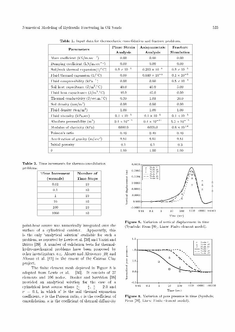
The thermo-elastic consolidation problem has beensolved by Aboustit et al. [28] and also by Lewis etal. [36]. In this case, a column of linear elastic materialis subjected to a unit surface pressure and a constantsurface temperature of T = 50�. Figure 4 shows the�nite element mesh of the problem. The pore pressureis kept equal to zero at the top surface; everywhere else,the boundaries of the soil are sealed and insulated (i.e.no uid or heat ow is permitted). The parametersused in the analysis are summarized in Table 1 and thetime steps used in the analysis are shown in Table 2.Almost the same temporal discretization shown inTable 2 was used in both studies by Aboustit et al. [28]and Lewis et al. [36], because this discretization schemeprovided good agreement with the analytical solutionfor `isothermal' consolidation problems [37].
All components in the coe�cient matrix shownin Equation 40 are included in this analysis, except[K31] and [K23]. This is done for reasons of comparisonwith the results of Aboustit et al. [28] and Lewis
Figure 4. Plane strain thermo-elastic consolidation.
et al. [36], in which these two matrices are set tozero. At the beginning of the analysis, a nine-pointintegration scheme was used to reduce oscillation inthe results. However, since no signi�cant improvementwas observed, a four-point integration scheme wasemployed.
The results are shown in Figures 5 to 7. Figure 5shows that displacements at nodes 7, 27 and 37 agreewell with the results obtained by Lewis et al. [36],except that the peak values are a little higher. Afterthe peak, displacements become negative (i.e. heave).The same result is reported by Lewis et al. [36] forvalues after the peak. Figure 6 shows the variationof calculated pore pressure, which clearly indicates thedissipation of pore pressure with time. However, theresults of this study show that the rate of pore pressuredissipation is slower than that reported by Lewis etal. [36]. It should be noted that calculating porepressure is the most di�cult part of the analysis, sinceit is very sensitive to time increment �t and oscillationmay occur at early times. Figure 7 demonstrates anexcellent match between the calculated temperature inthis study and those given by Lewis et al. [36].
Modeling Axisymmetric ThermalConsolidation Around a Buried Heat Source
The e�ects of a cylindrical radiating heat source, buriedin a thermo-elastic soil, were investigated by Bookerand Savvidou [38], where an analytic solution for a
Numerical Modeling of Hydraulic Fracturing in Oil Sands 525
Table 1. Input data for thermoelastic consolidation and fracture problems.
Parameters Plane StrainAnalysis
AxisymmetricAnalysis
FractureSimulation
Mass coe�cient (kN/m.sec�2) 0.00 0.00 0.00
Damping coe�cient (kN/m.sec�1) 0.00 0.00 0.00
Soil/rock thermal expansion(1/�C) 0:9� 10�6 0:203� 10�6 0:9� 10�6
Fluid thermal expansion (1/�C) 0.00 0:630� 10�5 0:1� 10�5
Fluid compressibility (kPa�1) 0.00 0.00 0:5� 10�3
Soil heat capacitance (J/m3.�C) 40.0 40.0 5.00
Fluid heat capacitance (J/m3.�C) 40.0 40.0 0.00
Thermal conductivity (J/sec.m.�C) 0.20 1.03 20.0
Soil density (ton/m3) 0.00 0.00 0.00
Fluid density (ton/m3) 1.00 1.00 1.00
Fluid viscosity (kPa.sec) 0:1� 10�5 0:1� 10�5 0:1� 10�5
Absolute permeability (m2) 0:4� 10�12 0:4� 10�11 5:5� 10�12
Modulus of elasticity (kPa) 6000.0 6000.0 0:6� 10+8
Poisson's ratio 0.40 0.40 0.40
Acceleration of gravity (m/sec2) 9.81 9.81 9.81
Initial porosity 0.1 0.1 0.3
� 1.00 1.00 1.00
Table 2. Time increments for thermo-consolidationproblems.
Time Increment(seconds)
Number ofTime Steps
0.01 10
0.1 10
1 10
10 10
100 10
1000 10
point-heat source was numerically integrated over thesurface of a cylindrical canister. Apparently, thisis the only `analytical solution' available for such aproblem, as reported by Lewis et al. [36] and Vaziri andBritto [39]. A number of validation tests for thermal-hydro-mechanical problems have been proposed byother investigators, e.g. Alonso and Alcoverro [40] andAlonso et al. [41] in the course of the Catsius Clayproject.
The �nite element mesh depicted in Figure 8 isadopted from Lewis et al. [36]. It consists of 27elements and 106 nodes. Booker and Savvidou [38]provided an analytical solution for the case of acylindrical heat source where a0
au = 14 , c
� = 2:0 and� = 0:4, in which a0 is the soil thermal expansioncoe�cient, � is the Poisson ratio, c is the coe�cient ofconsolidation, � is the coe�cient of thermal di�usivity
Figure 5. Variation of vertical displacement in time(Symbols: From [36], Lines: Finite element model).
Figure 6. Variation of pore pressure in time (Symbols:From [36], Lines: Finite element model).

526 A. Pak and D.H. Chan
Figure 7. Variation of temperature in time (Symbols:From [36], Lines: Finite element model).
Figure 8. Finite element mesh for axisymmetricthermo-elastic consolidation problem [36].
and au = �S(1 � �) + �w(�), where �S and �W arethe coe�cients of thermal expansion for solid particlesand uid, respectively, and � represents the porosity.The parameters used in the analysis are summarized inTable 1. The heat source was simulated by a constantheat input of 1000.0 J for both elements at the source.Temporal discretization is shown in Table 2.
Results are illustrated in Figures 9 to 11,which show horizontal displacements, pore pressures,and temperatures at three di�erent nodes, R/Ro=1,R/Ro=2, and R/Ro=5 shown in Figure 8 (Ro isthe radius of the cylindrical heat source). Figure 9indicates that displacements gradually increase up to acertain level, then, level o� and remain constant whenthe generated pore pressures are dissipated and thetemperatures have reached the steady state condition.Since changes in horizontal displacement have notbeen addressed in the analytical solution providedby Booker and Savvidou [38], in Figure 9 results
Figure 9. Comparison between analytical and numericalsolutions for horizontal displacements (Symbols: [36],Lines: Finite element model).
Figure 10. Comparison between analytical and numericalsolutions for pore pressure (Symbols: Analytical, Lines:Finite element model).
Figure 11. Comparison between analytical and numericalsolutions for temperature (Symbols: Analytical, Lines:Finite element model).
of the developed �nite element model are comparedwith those reported by Lewis et al. [36] for the sameproblem. Figure 10 shows the pore pressure gener-ation and dissipation caused by the radiating heatsource. For R/Ro=1, the time to reach the maximumpore pressure in the numerical solution is behind theanalytical one, but for R/Ro=2 and R/Ro=5, themaximum values occur at the same time and their

Numerical Modeling of Hydraulic Fracturing in Oil Sands 527
magnitudes are fairly close. Variation of temperaturewith time is shown in Figure 11, which indicates goodagreement between analytical and numerical solutions.It should be emphasized that the analytical results byBooker and Savvidou [38] do not provide the exactsolution for this problem, because of the di�erencebetween a point heat source and a cylindrical heatsource. Nevertheless, in their analytical solution, thedetermination of temperature was completely uncou-pled from that of the displacements and pore pres-sures.
The above example indicates that the results ofthe developed numerical model are satisfactory forcoupling of the three processes: Ground deformation, uid ow, and heat transfer.
Modeling of Thermally Induced Fracture
The analyses presented above illustrate the capabilityof the present model in simulating coupled thermalhydro-mechanical problems. In this section, the abilityof the model to simulate one-dimensional fracturepropagation will be examined and the node splittingfeature and activation of the fracture elements willbe demonstrated. Figure 12 shows the �nite elementmesh for the problem of thermally induced fracturein rock. As shown, the mesh consists of ten 8-node rectangular elements and four 6-node fractureelements. Double nodes were used in the middle rowfor modeling fracture propagation. Six-node fractureelements were introduced, but were not activated at thebeginning of the analysis. Also, a notch was provided,where uid with high pressure and temperature wasinjected into the medium. A uid ux of 10�6 m/secand a heat ux of 10.0 J/sec were applied inside thenotch. The initial pore pressure and temperature inthe material were set to zero. The material propertiesin this example are mentioned in Table 1. Generally,in the program, the induced stresses at the nodes areexamined to determine whether the tensile or shearfracture criterion is satis�ed. The criterion, which is
satis�ed �rst, would govern the type of fracture. Forinitiation of the fracture in this example, only thetensile strength criterion (for mode I fracture) has beenused. Also, the sti�ness of the fracture elements is setto zero.
Table 3 shows fracture propagation and activationof fracture elements at di�erent time steps. Figure 13shows the variation of pore pressure at nodes 18 and29 located at the injection boundary and at nodes1 and 45, which are located far from the injectionzone. It can be seen that pore pressures are generallyhigher at the injection point. Fracture elements areactivated after 6 seconds. Since the permeability ofthe fracture elements are set to ten times higher thanthe permeability of the soil matrix, the pore pressuredrops, because the uid suddenly �nds easier pathsto ow. After activation of all fracture elements, thepore pressure starts to increase again. The e�ects ofactivation of the fracture elements at nodes 1 and 45(which are located far from the injection boundaries)are not large, as expected. Variation of pore pressurealong the mesh and inside the induced fracture isdepicted in Figures 14 and 15, respectively. It should benoted that, due to activation of the fracture elements,the pore pressure at some nodes becomes negative.
Table 3. Fracturing sequence in time.
Time (sec.) Split Nodes Activated Elements
1 - -
2 - -
3 - -
4 - -
5 29 -
6 30 11
7 31, 32, 33 12
8 34, 35, 36, 37, 38 13, 14
9 - -
10 - -
Figure 12. Mesh for one-dimensional fracture propagation.

528 A. Pak and D.H. Chan
Figure 13. Variation of pore pressure at some nodes inthe soil and at the fracture.
Figure 14. Variation of pore pressure in the soil due tothe e�ect of fracturing.
Figure 15. Variation of pore pressure along the fracture.
However, these negative values decrease as the nodegets closer to the right boundary where a zero porepressure is imposed.
Figure 16 compares the variation of temperatureat node 18, which is located at the injection zone,and node 1, which is located far from the injectionarea. As expected, temperature at the injection zoneis higher. Variation of temperature along the meshand also inside the induced fracture is illustrated inFigures 17 and 18, respectively. As the �gures show,due to an injection of heated uid, the temperature
Figure 16. Variation of temperature in the soil and atthe fracture.
Figure 17. Variation of soil temperature due to theinjection of hot uid.
Figure 18. Variation of temperature along the fracturedue to the injection of hot uid.
is gradually and smoothly increasing toward a steadystate condition.
Modeling of Large Scale Hydraulic FractureLaboratory Experiments
A joint CANMET/industry/AOSTRA funded projectwas undertaken by Golder Associates to perform hy-draulic fracturing experiments in a large-scale triaxialchamber. The main objectives of the study were: (1)To provide a better understanding of the mechanism

Numerical Modeling of Hydraulic Fracturing in Oil Sands 529
Figure 19. Schematic view of large scale triaxial chamber (not to scale) from Golders Associates Report [42-44].
of hydraulic fracture formation and propagation inuncemented oil sands under conditions of high leak-o� and (2) To determine the e�ect of uid injectionrate and, also, the in uence of di�erent stress �eldson the fracturing process. These experiments werecarried out in a large triaxial stress chamber, shownschematically in Figure 19, which can accommodatesamples of up to 1.00 meter high and 1.40 meter indiameter. Quartz sand was used in these experiments,which was saturated with a viscous uid, such as invertliquid sugar instead of oil, and injected with dyed invertliquid sugar (phases I and II) and dyed water (phaseIII), in order to trace the fracture. Figure 19 showsa hollow steel pipe, with an outside diameter of 33.5mm and perforated at mid-height, which was used tosimulate the injection well. Principal stresses of up to1000 kPa could be applied independently in the vertical(�v) and radial (�h) directions, as illustrated in the�gure.
Lane Mountain 125 quartz sand was chosen forthe laboratory tests. Its behavior was reported to besimilar to oil sand, which exhibits high dilatancy andpost peak softening during triaxial compression underlow e�ective con�ning stresses. The speci�c gravity ofLane Mountain sand grain was determined to be 2.65and its permeability was measured to be 4:56 � 10�3
cm/sec to water and 4:0�10�6 cm/sec to liquid sugar.
Boundary conditions were free draining at the topand bottom of the chamber, which were connected toa constant pressure equal to +200 kPa. No radialdrainage was allowed.
At the end of each test, the sample was excavatedin horizontal lifts, normally 1.5 to 3.0 cm in thickness,under black light. When each lift was completelyexcavated, the locations of the dye were marked withblack string and, then, a normal photograph was takenunder normal light [42-44].
In this study, test 4 of phase II experimentswas selected for numerical modeling. The sampledimensions and position of instrumentation are shownin Figures 20 and 21. Two permeability tests carriedout on the saturated sample gave permeability values of4.9 and 4.6 Darcys. Horizontal and vertical boundarytractions of 600 kPa and 400 kPa, respectively, wereapplied on the sample, with a back pressure of 200 kPato keep the sample fully saturated. The K0(= �0h=�0v)value was equal to 2 for this test, which indicated thathorizontal fracture planes were expected. In this test,250 ml of dyed liquid sugar were injected into the testsample in 8.3 seconds (30 ml/sec.).
A �nite element mesh comprised of 704 elements(260 eight-node rectangular elements and 444 six-node fracture elements) with 1562 nodes (including thedouble nodes) was used. Due to the axial symmetry

530 A. Pak and D.H. Chan
Figure 20. Plan view of instrumentation around theinjection zone.
Figure 21. Sample dimensions and position ofpiezometers for test #4 of phase 2 of the experiments.
of the problem, only half the sample was analyzed, asshown in Figure 22. The boundary conditions were:
� Bottom boundary: Fixed in the horizontal andvertical directions, free drainage,
� Top boundary: Free, free drainage,� Left boundary: Fixed in the horizontal direction, no
drainage allowed,� Right boundary: Free, no drainage allowed.
An important aspect of the coupling process is�nding an appropriate value for time increment, �t,suitable for all �eld equations. Due to the high speedof stress waves in soil/rock, the time increment in theequilibrium equation should be small enough to capturethe behavior of soil/rock accurately. On the other
Figure 22. Finite element mesh and boundary conditionsfor modeling test 4 of phase 2.
hand, the time increment cannot be very small becausethe coupled analysis of the consolidation phenomenonrequires that �t be larger than some certain value in or-der to avoid instability and spurious oscillations [45,46].The time increment for this analysis was chosen to beone second.
An axisymmetric analysis was carried out consid-ering the linear elastic behavior for sand with an elasticmodulus equal to 41050 kPa and a Poisson ratio of 0.25.These values were obtained from small scale triaxialtests on Lane Mountain sand. The permeability ofthe fracture elements was considered to be 100 timesgreater than the surrounding soil matrix (100 ksoil). Inthis analysis, nodal coordinates were not updated and anominal thickness equal to 2 mm was considered for thefracture elements. This is close to the width of the realfractures in oil sands, which is 3 to 5 mm [13]. A listof the parameters used in the analysis is summarizedin Table 4.
The test was simulated by injecting uid at theperforated area of the wellbore. An injection rate of30 ml/sec in this test is equal to an injection ux of0.0052 m/sec when divided by the perforated area. Thevariation of pore uid pressure at the injection zoneis shown in Figure 23. Although the calculated peakpressure is slightly higher than the measured pressure,the overall behavior is very similar. The initial slopesof the two curves are di�erent; this is because, in the�nite element analysis, the stresses were examined atthe end of each time step to identify the possibilityof fracture. For instance, if the time increment is 1second, no fracturing will occur until the end of thetime increment. Obviously, in reality, fractures can

Numerical Modeling of Hydraulic Fracturing in Oil Sands 531
Table 4. List of parameters for modeling of thermo-elastic consolidation and hydraulic fracture problems.
ParametersHydraulicFractureProblem
Mass coe�cient (kN/m.sec�2) 0.00
Damping coe�cient (kN/m.sec�1) 0.00
Soil/rock thermal expansion (1/�C) -
Fluid thermal expansion (1/�C) -
Fluid compressibility (kPa�1) 0:3� 10�5
Soil heat capacitance (J/m3.�C) -
Fluid heat capacitance (J/m3.�C) -
Thermal conductivity (J/sec.m.�C) -
Soil density (ton/m3) 2.0
Fluid density (ton/m3) 1.33
Fluid viscosity (kPa.sec) 1:49� 10�3
Absolute permeability (m2) 4:48� 10�12 � 4:48� 10�10
Modulus of elasticity (kPa) 41050.0
Poisson's ratio 0.25
Acceleration of gravity (m/sec2) 9.81
Initial porosity 0.48
� 1.00
Figure 23. Comparison between calculated and measuredpore pressures (piezometer: At injection zone).
occur in a fraction of second, resulting in a higher rateof ow and lower pressure.
As seen in Figure 23, there is a jump in the porepressure at the beginning of injection, followed by afairly constant pore pressure during the injection. Atthe end of injection, both calculated and measuredcurves show a decline in pore pressure, which representsthe consolidation phenomenon.
Pore pressures at the piezometers, installed at adistance of 75 mm from the injection pipe (Figures 20and 21), are compared to the numerical solution in
Figure 24. Comparison between pore pressure variationof lab experiment and numerical model at the piezometer(100 mm above the injection zone).
Figures 24 and 25. Piezometers were installed at threelevels, but the lower one did not show a signi�cantchange in pore pressure. A good agreement betweenthe numerical results and measured values in thelaboratory can be observed.
The fracture pattern obtained from the numericalmodel is shown in Figure 26. The sequence shows thefracture pattern at the onset of injection, 4 seconds af-ter starting injection, 8 seconds after starting injection(end of injection), and at 30 seconds. The numericalmodel showed a fracture zone, which gradually ex-

532 A. Pak and D.H. Chan
Figure 25. Comparison between pore pressure variationof lab experiment and numerical model at the piezometers(100 mm below the injection zone).
Figure 26. Pattern of fracture propagation fromnumerical model.
panded with injection. The actual fracture pattern ob-served in the laboratory is shown in Figure 27. Despitethe fact that Ko =2.0, neither the numerical model northe experimental results showed the anticipated planarfracture. Studies on pore pressure distribution insidethe medium indicated that fracture occurs at placeswith higher pore pressure. In other words, the contoursof higher pore pressure can approximately determinethe zone of fracturing [47].
Fracture Propagation in an ElastoplasticMaterialIn petroleum engineering, it is known that the com-pressibility of oil sand is nonlinear at low stresses(e.g. [14] ). In geotechnical terms, this basicallymeans that the stress-strain behavior of oil sand isnonlinear and its bulk modulus (sti�ness) varies withchanges in stress. Some researchers have considered anonlinear elastic (hyperbolic) model for simulating thisbehavior [48], while others have proposed an elasto-plastic constitutive model (e.g. [49]). In this study, inorder to evaluate the e�ects of soil failure on fracturepatterns in isothermal conditions, an associated Mohr-Coulomb model was employed. This model is capableof simulating high dilation, which is an importantcharacteristic of oil sand. In this model, the following
Figure 27. Fracture pattern form laboratory experimentreproduced form Golder Associate Report [43].
parameters were used:
Cp = 0; Cr = 0;�p = 38�; �r = 38�;E = 41050 kPa; � = 0:25;
where Cp is the peak cohesion, Cr is the residual co-hesion, �p represents the peak friction angle, �r meansthe residual friction angle and E and � represent themodulus of elasticity and Poisson ratio, respectively.
Boundary tractions of 600 kPa horizontal and 400kPa vertical, with 200 kPa back pressure were appliedon the sample. According to the Mohr-Coulomb failurecriterion, the ratio of the principal stresses at yieldingis given by:
�1 � �3
2=�1 + �3
2sin�+ C cos�: (42)
For C = 0 and � = 38�;�1 � �3
2=�1 + �3
2sin 38� ! �1
�3= 4:2:
Hence, at places where this ratio applies, soil becomesplastic and stresses and pore pressures are a�ected,accordingly. The pore pressure variation at the injec-tion zone is shown in Figure 28. In this �gure, theresults of the analysis, with di�erent permeabilities forthe fracture elements (500 and 1000 times greater thanthe permeability of the surrounding soil), are included.In general, the initial pore pressure in this case shows

Numerical Modeling of Hydraulic Fracturing in Oil Sands 533
Figure 28. Pore pressure variation at the injection zonewith di�erent permeabilities for fracture elements.
around 30% higher pore pressure compared to theelastic case. The e�ect of increasing the permeabilityof fracture elements on reducing pore pressure can beobserved in this �gure.
Fracture patterns for elastoplastic analysis aredepicted in Figure 29. Compared to the fracturepatterns of elastic analysis, they are less dispersedand the fracture zones are smaller. The numericalmodel, in this case, indicates that tensile and shearfractures can simultaneously occur in the hydraulicfracturing process. Despite the fact that the shearfailure zone is small, the dilation characteristics ofthe material will generate compressive stresses in acon�ned condition, which can inhibit fracture growth.This explains why there is a less dispersed fracture zonein the elastoplastic analysis.
CONCLUSIONS
A fully coupled thermal hydro-mechanical fracture�nite element model is developed, which is able tosimulate the process of hydraulic fracturing underisothermal and non-isothermal conditions. The mod-eling of large scale hydraulic fracturing laboratoryexperiments in uncemented porous materials, such assand, has provided results, which are in agreementwith experimental observations. In this model, the
Figure 29. Fracture pattern with associatedMohr-Coulomb model.
importance of the amount of pore pressure and itsdistribution is emphasized in the process of hydraulicfracturing in uncemented porous materials. The frac-ture pattern is roughly similar to the contours of highpore pressure. The numerical model shows that achange in the permeability of soil and/or fractures hasa drastic e�ect on the variation of pore pressure andthe resulting fracture pattern.
The model establishes that, in uncemented porousmaterials, tensile and shear fractures can occur si-multaneously. The numerical model and laboratoryexperiments both indicate that, for uncemented porousmaterials, such as oil sands, a simple planar fracture isunlikely to occur and a system of multiple fractures ora fracture zone consisting of interconnected tiny cracksshould be expected.
ACKNOWLEDGMENT
The authors wish to thank CANMET, Imperial Oil Re-sources Canada Ltd., Shell Canada Ltd., Japan CanadaOil Sands Ltd., AOSTRA, and Golder Associates Ltd.for providing the experimental data for this research.
NOMENCLATURE
�ij stress tensor at a pointFi external load vectorUi displacement vector i.e. hu v wiTm0 mass coe�cientc0 damping coe�cienti; j indices taking 1, 2 and 3 representing
coordinate axes! weighting factornj unit vector normal to the surfaceS surface boundaryV volume�0ij e�ective stress tensor (tension positive)�P change in pore uid pressure
(compression positive)�ij Kronecker deltaDijkl soil/rock constitutive matrix"kl (total) strain tensor�S coe�cient of thermal expansion for
soil/rock (porous matrix)�T change in temperature� density of uidv velocity vector of owing uidG uid mass output (sink) or input
(source)� porosity of soil mass

534 A. Pak and D.H. Chan
t timer del operator�S coe�cient of thermal expansion for
soil/rock�P coe�cient of thermal expansion for
uid�T uid compressibility"V volumetric strainLe volumetric thermal energy uxE internal energy per unit mass� uid densityQ energy input (source) or output (sink)
per unit volumet time� porosity of soil/rock matrix�S soil/rock densityCs heat capacity of soil/rock�f uid densityS degree of saturation� coe�cient of conductivityfi volumetric ux of owing uidg acceleration of gravityz elevationJ mechanical equivalent of heatCv heat capacity of uid at constant
volumeCp heat capacity of uid at constant
pressureT temperatureTo initial temperature
REFERENCES
1. Veatch, R.W., Moschovidis, Z.A. and Fast, C.R. \Anoverview of hydraulic fracturing", in Recent Advancesin Hydraulic Fracturing; SPE Monograph, 12, pp 2-38(1989).
2. Zheltov, Y.P. and Khristianovitch, S.A. \On themechanism of hydraulic fracturing of an oil-bearingstratum", Izvest. Akad. Nauk SSR, OTN, 5, pp 3-41(in Russian) (1995).
3. Perkins, T.K. and Kern, L.R. \Width of hydraulicfractures", JPT, Trans., AIME, 222, pp 937-49 (1961).
4. Geertsma, J. and Deklerk, F.A. \Rapid method ofpredicting width and extent of hydraulically inducedfractures", JPT, Trans., AIME, 246, pp 1571-81(1969).
5. Nordgren, R.P. \Propagation of a vertical hydraulicfracture", SPEJ, Trans., AIME, 253, pp 306-14(1972).
6. Clifton, R.J. and Abou-Sayed, A.S. \A variationalapproach to the prediction of the three-dimensionalgeometry of hydraulic fractures", Paper SPE 9879presented at the 1981 SPE/DOE Low PermeabilitySymposium (1981).
7. Clifton, R.J. \Recent advances in the three dimen-sional simulation of hydraulic fracturing", Develop-ments in Mechanics, Proc. 19th Mid-Western Mechan-ics Conference, Ohio State U., Columbus, 13, pp 311-319 (1985).
8. Advani, S.H., Lee, T.S. and Lee, J.K. \Three dimen-sional modeling of hydraulic fractures in layered media:Part I- �nite element formulations", Journal of EnergyResources Technology, 112, pp 1-19 (1990).
9. Advani, S.H. and Lee, J.K. \Finite element model sim-ulations associated with hydraulic fracturing", SPEJ,Trans., AIME, 22, pp 209-218 (1982).
10. Settari, A. and Raisbeck, J.M. \Fracture mechanicsanalysis in in-situ oil sand recovery", JCPT, pp 85-94(1979).
11. Settari, A. and Raisbeck, J.M. \Analysis and nu-merical modeling of hydraulic fracturing during cyclicsteam stimulation in oil sands", JPT, pp 2201-2212(1981).
12. Atukorala, U.D. \Finite element analysis of uidinduced fracture behavior in oil sand", M.Sc. the-sis, Dept. of Civil Engineering, University of BritishColombia (1983).
13. Settari, A., Kry, P.R. and Yee, C.-T. \Coupling of uid ow and soil behavior to model injection intouncemented oil sands", JCPT, 28(1), pp 81-92 (1989).
14. Settari, A. \Physics and modeling of thermal ow andsoil mechanics in unconsolidated porous media", SPE18420, pp 155-169 (1989).
15. Settari, A., Ito, Y. and Jha, K.N. \Coupling of afracture mechanics model and a thermal reservoir sim-ulator for tar sands", JCPT, 31(2), pp 20-27 (1992).
16. Frydman, M. and Fontoura, S. \Numerical modelingof borehole pressurization", International Journal ofRock Mechanics and Mining Sciences, 34(3-4) (1997).
17. Ouyang, G., Carey, G.F. and Yew, C.H. \Adaptive�nite element scheme for hydraulic fracturing withproppant transport", International Journal for Nu-merical Methods in Fluids, 24(7), pp 645-670 (1997).
18. Itaoka, M., Sato, K. and Hashida, T. \Numericalsimulation of geothermal reservoir formation inducedby hydraulic fracturing at great depth", Transactions-Geothermal Resources Council, pp 297-302 (2002).
19. Yang, T.H., Li, L.C., Tam, L.G. and Tang, C.A.\Numerical approach to hydraulic fracturing in het-erogeneous and permeable rocks", Key EngineeringMaterials, 243-244, pp 351-356 (2003).
20. Reynolds, M., Shaw, J. and Pollock, B. \Hydraulicfracture design optimization for deep foothills gaswells", Journal of Canadian Petroleum Technology,43(12), pp 5-10 (2004).
Numerical Modeling of Hydraulic Fracturing in Oil Sands 535
21. Lu, L.J., Sun, F.C., Xiao, H.H. and An, S.F. \NewP3D hydraulic fracturing model based on the radial ow", Journal of Beijing Institute of Technology (En-glish Edition), 13(4), pp 430-435 (2004).
22. Cook, B.K., Lee, M.Y., DiGiovanni, A.A., Bronowski,D.I., Perkins, F.D. and Williams, J.R. \Discrete el-ement modeling applied to laboratory simulation ofnear well-bore mechanics", International Journal ofGeomechanics, 4(1), pp 19-27 (2004).
23. Carter, R.D. \Appendix to: Optimum uid charac-teristics for fracture extension", by G.C. Howard andC.R. Fast, Drill and Prod. Prac., API 267 (1957).
24. Zienkiewicz, O.C. and Taylor, R.L., The Finite Ele-ment Method, 4th Ed., 2, McGraw-Hill (1991).
25. Zienkiewicz, O.C., Chan, A.H.C., Pastor, M., Schre- er, B.A. and Shiomi, T. Computational Geomechan-ics, with Special Reference to Earthquake Engineering,Chapter 3, John Wiley & Sons (1998).
26. Christian, J.T. \ Two and three dimensional con-solidation", in Numerical Methods in GeomechanicalEngineering, C.S. Desai and J.T. Christian, Eds., pp399-426, London, McGraw-Hill (1977).
27. Johnston, P.R. \Finite element consolidation analysisof tunnel behavior on clay", Ph.D. Thesis, StanfordUniversity (1981).
28. Aboustit, B.L., Advani, S.H. and Lee, J.K. \Vari-ational principles and �nite element simulations forthermo-elastic consolidation", Int. J. Num. Anal.Meth. Geomech., 9, pp 49-69 (1985).
29. Thomas, G.W., Principles of Hydrocarbon ReservoirSimulation, Tabir Publishers (1977).
30. Pratts, M. \Thermal recovery", SPE Monograph No.,(1982).
31. Pak, A. \Numerical modeling of hydraulic fracturing",Ph.D. Thesis, Department of Civil and EnvironmentalEngineering, University of Alberta, Canada (1997).
32. Daneshy, A.A. \On the design of vertical hydraulicfractures", Petroleum Engineers Journal, pp 61-68(April 1973).
33. Wiles, T.D. and Roegiers, J.C. \Modeling of hydraulicfractures under in-situ conditions using a displacementdiscontinuity approach", Proceedings, 33rd AnnualTechnical Meeting of the Petroleum Society of CIM,Paper No. 82-33-70 (June 6-9, 1982).
34. Witherspoon, P.A., Wang, J.S.Y., Iwai, K. and Gale,J.E. \Validity of cubic law for uid ow in a deformablerock fracture", Water Resources Research, 16(6), pp1016-1024 (1980).
35. Ryan, T.M., Farmer, I.W. and Kimbrell, A.F. \Lab-oratory determination of fracture permeability", Pro-ceedings of the 28th U.S. Symposium of Rock Mechan-ics, Tucson, pp 593-600 (1987).
36. Lewis, R.W., Majorana, C.E. and Schre er, B.A. \Acoupled �nite element model for the consolidation ofnonisothermal elastoplastic porous media", Transportin Porous Media, 1, pp 155-178 (1986).
37. Sandhu, R.S. \Finite element analysis of soil con-solidation", National Science Foundation Grant No.72-04110-A, Geotechnical Engineering Report No.6,Dept. of Civil Engineering, The Ohio State University,Columbus, Ohio (1976).
38. Booker, J.R. and Savvidou, C. \Consolidation arounda point heat source", Int. J. for Numerical and Analyt-ical Methods in Geomechanics, 9, pp 173-184 (1985).
39. Vaziri, H.H. and Britto, A.M. \Theory and applica-tion of a fully coupled thermo-hydro-mechanical �niteelement model", SPE, 25306 (1992).
40. Alonso, E. and Alcoverro, J., Catsius Clay Project.Calculations and Testing of Behavior of UnsaturatedClay as Barrier in Radioactive Waste Repositories,ENRESA Technical Publication 10/99 (1999).
41. Alonso, E. et al., Febex. Proportional Thermo-Hydro-Mechanical (THM) Modeling of In-Situ Test, ENRESATechnical Publication 09/98 (1998).
42. Golders Associates Ltd. \Laboratory simulation andconstitutive behavior for hydraulic fracture propaga-tion in oil sands, phase I", Project No. 902-2013 (1991).
43. Golder Associates Ltd. \Laboratory simulation andconstitutive behavior for hydraulic fracture propaga-tion in oil sands, phase II", Project No. 912-2055,(1992).
44. Golder Associates Ltd. \Laboratory study of hydraulicfracture propagation in oil sands, phase III", ProjectNo. 932-2005 (1994).
45. Gatmiri, B. and Magnin, P. \Minimum time stepcriterion in FE analysis of unsaturated consolidation:Model UDAM", Proc. 3rd European Spec. Conf. onNum. Meth. in Geo. Eng., Manchester, UK (1994).
46. Song, E.X. \Time step size in �nite element analysisof consolidation", Proc. 3rd European Spec. Conf. OnNum. Meth. in Geo. Eng., Manchester, UK (1994).
47. Pak, A. and Chan. D.H. \A fully implicit single phaseT-H-M fracture model for modeling hydraulic frac-turing in oil sands", Journal of Canadian PetroleumTechnology, 43(6), pp 35-44 (2004).
48. Vaziri, H.H. \Nonlinear temperature and consolidationanalysis", Ph.D. Thesis, Department of Civil Engineer-ing, University of British Columbia (1986).
49. Wan, R., Chan, D.H. and Kosar, K.M. \A constitutivemodel for the e�ective stress-strain behavior of oilsands", Pet. Soc. CIM, Paper No. 89-40-66, 40th ATMof CIM, Ban� (1989).


