Evaluation of urea–ammonium–nitrate fertigation with drip irrigation using numerical modeling Blaine R. Hanson a , Jirka S ˇ imu ˚ nek b , Jan W. Hopmans a, * a LAWR, University of California, 123 Veihmeyer Hall, Davis, CA 95616, United States b Environmental Sciences, University of California, Riverside, CA, United States 1. Introduction Microirrigation with fertigation provides an effective and cost- efficient way to supply water and nutrients to crops (Bar- Yosef, 1999). However, less-than-optimum management of microirrigation systems resulting in excessive water and nitrogen applications may result in inefficient water and nutrient use, thereby diminishing expected yield benefits and contributing to ground water pollution. The quality of soils, ground, and surface waters is specifically vulnerable in climatic regions where agricultural production occurs mostly by irrigation, such as in California. Liquid nitrogen (N) fertigation, using mixtures of urea, ammonium, and nitrate compounds, is widely used with microirrigation. Robust guidelines for managing microirrigation systems are needed so that the principles of sustainable agriculture are satisfied. agricultural water management 86 (2006) 102–113 article info Article history: Accepted 12 June 2006 Published on line 30 August 2006 Keywords: Irrigation Nitrogen management Microirrigation Nitrate leaching abstract Microirrigation with fertigation provides an effective and cost-efficient way to supply water and nutrients to crops. However, less-than-optimum management of microirrigation sys- tems may cause inefficient water and nutrient use, thereby diminishing expected yield benefits and contributing to ground water pollution if water and nitrogen applications are excessive. The quality of soils, ground, and surface waters is specifically vulnerable in climatic regions where agricultural production occurs mostly by irrigation such as in California. Robust guidelines for managing microirrigation systems are needed so that the principles of sustainable agriculture are satisfied. The main objective of this research was to use an adapted version of the HYDRUS-2D computer model to develop irrigation and fertigation management tools that maximize production, yet minimize adverse environ- mental effects. This software package can simulate the transient two-dimensional or axi- symmetrical three-dimensional movement of water and nutrients in soils. In addition, the model allows for specification of root water and nitrate uptake, affecting the spatial distribution of water and nitrate availability between irrigation cycles. Recently, we ana- lyzed four different microirrigation systems in combination with five different fertigation strategies for various soil types using a nitrate-only fertilizer, clearly demonstrating the effect of fertigation strategy on the nitrate distribution in the soil profile and on nitrate leaching. In the present study, the HYDRUS-2D model was used to model the distribution of soil nitrogen and nitrate leaching using a urea–ammonium–nitrate fertilizer, commonly used for fertigation under drip irrigation. In addition, the distribution of phosphorus and potassium was modeled. Model simulations are presented for surface drip and subsurface drip tape, each associated with a typical crop in California. # 2006 Elsevier B.V. All rights reserved. * Corresponding author. Tel.: +1 530 752 3060; fax: +1 530 752 5262. E-mail addresses: [email protected](B.R. Hanson), [email protected](J. S ˇ imu ˚ nek), [email protected](J.W. Hopmans). available at www.sciencedirect.com journal homepage: www.elsevier.com/locate/agwat 0378-3774/$ – see front matter # 2006 Elsevier B.V. All rights reserved. doi:10.1016/j.agwat.2006.06.013
Transcript
Evaluation of urea–ammonium–nitrate fertigation withdrip irrigation using numerical modeling
Blaine R. Hanson a, Jirka Simunek b, Jan W. Hopmans a,*a LAWR, University of California, 123 Veihmeyer Hall, Davis, CA 95616, United StatesbEnvironmental Sciences, University of California, Riverside, CA, United States
a g r i c u l t u r a l w a t e r m a n a g e m e n t 8 6 ( 2 0 0 6 ) 1 0 2 – 1 1 3
a r t i c l e i n f o
Article history:
Accepted 12 June 2006
Published on line 30 August 2006
Keywords:
Irrigation
Nitrogen management
Microirrigation
Nitrate leaching
a b s t r a c t
Microirrigation with fertigation provides an effective and cost-efficient way to supply water
and nutrients to crops. However, less-than-optimum management of microirrigation sys-
tems may cause inefficient water and nutrient use, thereby diminishing expected yield
benefits and contributing to ground water pollution if water and nitrogen applications are
excessive. The quality of soils, ground, and surface waters is specifically vulnerable in
climatic regions where agricultural production occurs mostly by irrigation such as in
California. Robust guidelines for managing microirrigation systems are needed so that
the principles of sustainable agriculture are satisfied. The main objective of this research
was to use an adapted version of the HYDRUS-2D computer model to develop irrigation and
fertigation management tools that maximize production, yet minimize adverse environ-
mental effects. This software package can simulate the transient two-dimensional or axi-
symmetrical three-dimensional movement of water and nutrients in soils. In addition, the
model allows for specification of root water and nitrate uptake, affecting the spatial
distribution of water and nitrate availability between irrigation cycles. Recently, we ana-
lyzed four different microirrigation systems in combination with five different fertigation
strategies for various soil types using a nitrate-only fertilizer, clearly demonstrating the
effect of fertigation strategy on the nitrate distribution in the soil profile and on nitrate
leaching. In the present study, the HYDRUS-2D model was used to model the distribution of
soil nitrogen and nitrate leaching using a urea–ammonium–nitrate fertilizer, commonly
used for fertigation under drip irrigation. In addition, the distribution of phosphorus and
potassium was modeled. Model simulations are presented for surface drip and subsurface
drip tape, each associated with a typical crop in California.
The partial differential equations governing two-dimen-
sional nonequilibrium chemical transport of solutes involved
in a sequential first-order decay chain during transient water
flow in a variably saturated rigid porous medium are:
@uc1
@tþ r
@s1
@t¼ @
@xiuDi j;1
@c1
@xj
!� @qic1
@xi
� mw;1uc1 � ms;1rs1 � Scr;1 (2)
@uck@tþ r
@sk@t¼ @
@xiuDi j;k
@ck@x j
!� @qick
@xi� mw;1uck � ms;krsk
þ mw;k�1uck�1 þ ms;k�1rsk�1 � Scr;k; k e ð2; nsÞ (3)
where c and s are solute concentrations in the liquid [M L�3]
and solid [M M�1] phases, respectively; qi the ith component of
the volumetric flux density [L T�1], mw and ms first-order rate
constants for solutes in the liquid and solid phases [T�1],
respectively, providing connections between individual chain
species, r the soil bulk density [M L�3], S the sink term
[L3 L�3 T�1] in the water flow equation (Eq. (1)), cr the concen-
tration of the sink term [M L�3], Dij the dispersion coefficient
tensor [L2 T�1] for the liquid phase, subscript k the kth chain
number, and ns is the number of solutes involved in the chain
reaction. The last term in both equations represents passive
nutrient uptake through the product of root water uptake, S,
and species concentration.
The adsorption isotherm relating sk and ck is described by a
linear equation of the form
sk ¼ Kd;kck (4)
where Kd,k [L3 M�1] is the distribution coefficient of species k.
Eq. (2) represents either the first species in the chain
reaction (urea) or an independent species (P and K), while
Eq. (3) represents second and other solutes in the sequential
first-order decay chain (ammonium and nitrate). Note that the
first-order decay coefficient m acts as sink in Eq. (2) and as a
source in Eq. (3). Relative concentrations can be used since all
transport and reaction parameters (Kd, m) are concentration
independent and thus both transport equations are linear.
2.3. Parameter values and boundary conditions
2.3.1. Parameter valuesUrea (Eq. (2)), ammonium and nitrate (Eq. (3)) were considered
for the nitrogen species simulations. While urea and nitrate
were assumed to be present only in the dissolved phase (i.e.,
Kd = 0 cm3 g�1), ammonium was assumed to adsorb to the solid
phase using a distribution coefficient Kd of 3.5 cm3 g�1. Similar
values were reported in the literature: Kd = 3–4 cm3 g�1 by Lotse
et al. (1992), Kd = 1.5 cm3 g�1 by Selim and Iskandar (1992), and
Kd = 3.5 cm3 g�1 by Ling and El-Kadi (1998). The first-order decay
coefficient mw for urea, representing hydrolysis, was set to be
a g r i c u l t u r a l w a t e r m a n a g e m e n t 8 6 ( 2 0 0 6 ) 1 0 2 – 1 1 3106
0.38 day�1. Again, similar values were used in the literature, for
example by Ling and El-Kadi (1998) who considered hydrolysis
to be in the range of 0.36, 0.38, and 0.56 day�1. Nitrification from
ammonium to nitrate was modeled using the rate coefficient of
0.2 day�1, which represents the center of the range of values
reported in the literature, e.g., 0.2 day�1 by Jansson and Karlberg
(2001), 0.02–0.5 day�1 by Lotse et al. (1992), 0.226–0.432 day�1 by
Selim and Iskandar (1992), 0.15–0.25 day�1 by Ling and El-Kadi
(1998), and 0.24–0.72 day�1 by Misra et al. (1974). Volatilization of
ammonium and subsequent ammonium transport by gaseous
diffusion was neglected.
Although HYDRUS-2D allows for denitrification, the pre-
sented simulations did not account for any denitrification to
occur. Although we included denitrification initially, results
were unsatisfactory because of the large sensitivity of
denitirification rates on the model results; yet little informa-
tion on denitrification rate as a function of the soil moisture
regime under drip irrigation is available. Therefore, denitri-
fication was not considered at this time.
There is also relatively large uncertainty concerning the
values of the distribution coefficients for phosphorus and
potassium. In our simulations we used values derived from
Silberbush and Barber (1983), i.e., Kd = 59.3 cm3 g�1 for phos-
phorus and 28.7 cm3 g�1 for potassium. For phosphorus, this is
in the range of 19 cm3 g�1 reported by Kadlec and Knight (1996)
and of 185 cm3 g�1 reported by Grosse et al. (1999). We
assumed that the bulk density was equal to 1.5 g cm�3, the
longitudinal dispersivity was equal to 5 cm, with the trans-
verse dispersivity being one-tenth of the longitudinal dis-
persivity, and neglected molecular diffusion as it was
considered negligible relative to dispersion.
2.3.2. Initial and boundary conditionsEach of the fertigation scenarios was preceded by 56 days of
flow-only simulations, to approach a ‘pseudo-equilibrium’
condition before irrigation with fertigation started. This was
done to ensure that the initial soil water regime was not a
factor in the transport and leaching predictions (Gardenas
et al., 2005). The initial condition for this initialization period
was set to a uniform soil water pressure head of �400 cm. The
soil hydraulic parameters of the van Genuchten (1980) model
for the loam were taken from Carsel and Parrish (1988). The
transport domain was considered to be solute free at the
beginning of the fertigation simulation.
All boundaries were assumed to be no flow boundaries with
the exception of the bottom of the soil profile and the boundary
representing the irrigation device. A unit gradient boundary
condition for water flow and the Neumann boundary condition
for solute transport were used at the bottom of the soil profile.
System dependent boundary conditions representing irrigation
devices were described in detail by Gardenas et al. (2005) and are
listed in Table 1. The selected parameters for the Feddes et al.
(1978) water stress response function were taken from van Dam
et al. (1997), and are presented in Table 1 as well. Root
distribution in the soil profile was assumed to be described
using Vrugt’s model (Vrugt et al., 2001). The values of the root
distribution parameters in Table 1 reflect typical root systems
for the two irrigated cropping systems and were introduced by
Gardenas et al. (2005) to represent maximum rooting depths of
about 100 cm.
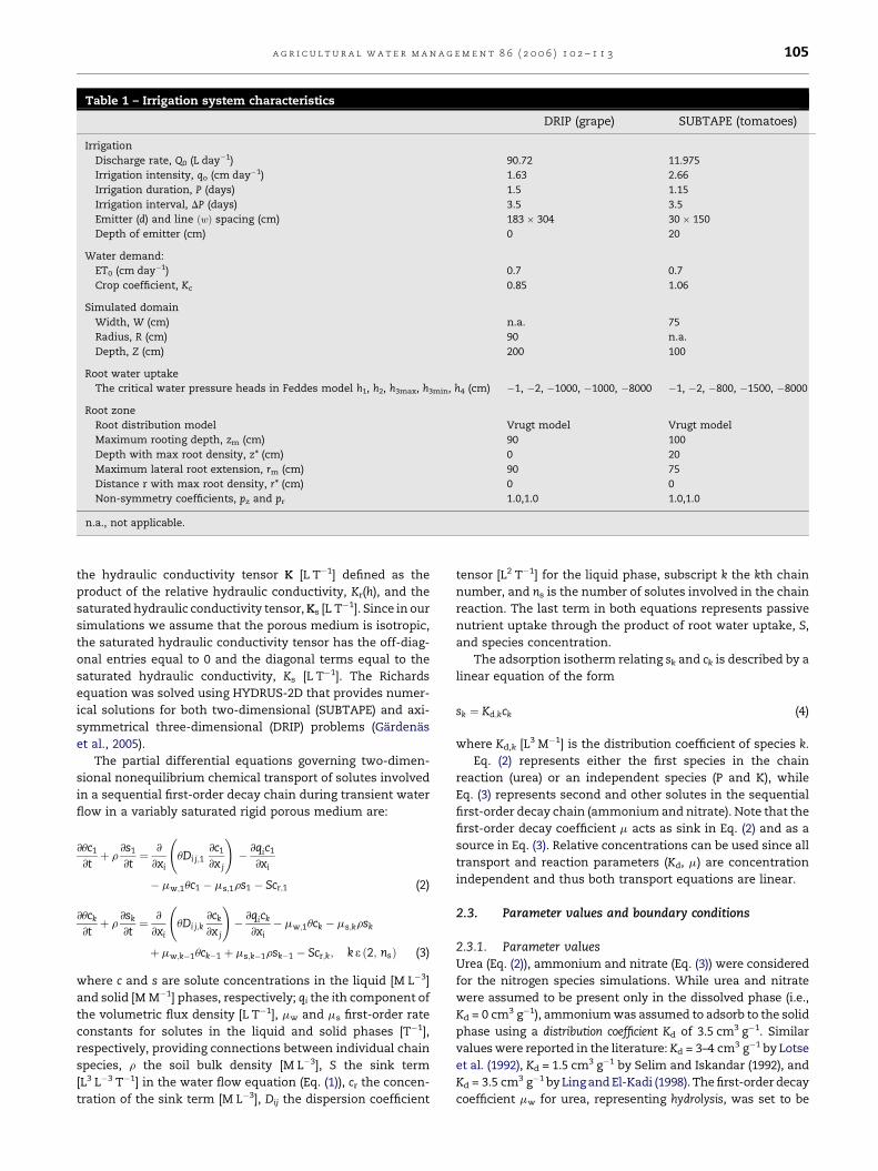
2.3.3. Irrigation system parametersThe irrigation requirement, Qreq (L day�1), was computed from
the crop-specific potential evapotranspiration (ETc) (cm day�1)
and the irrigated soil area, A ¼ dw, where d (cm) and w (cm)
represent emitter distance and irrigation line distance,
respectively. Selected ETc values are typical values for
California irrigated crops. The model also included an
evaporation component for the DRIP simulations (Gardenas
et al., 2005). The applied irrigation volume per irrigation cycle, I
[cm3], was estimated for each crop from Qreq, the irrigation
interval, DP [days], and the irrigation efficiency, fi. For all
irrigation systems, we assumed an irrigation efficiency of 85%
(Hanson, 1995). Thus, plant water uptake was less than the
applied water for all scenarios. Finally, the irrigation cycle
duration, P (day�1), was determined from the total irrigation
volume, I, and the emitter discharge rate, Qo. Specific values
for each of the two studied microirrigation systems are
presented in Table 1.
2.4. Fertigation scenarios
Similar to the study of Gardenas et al. (2005), we considered
three fertigation strategies to evaluate water and nutrient
use efficiency and nitrate leaching. These are based on
recommendations of the microirrigation industry and
grower’s practices. These are (B) fertigation for a total
duration of 2 h, starting 1 h after the beginning of the
irrigation cycle; (E) fertigation for a duration of 2 h, starting
3 h before the end of the irrigation cycle; and (M50), starting
the first and last 25% of each irrigation with fresh water, and
fertigation during the remaining 50% in the middle of the
irrigation cycle. The fresh water irrigations prior and after
each fertigation are common practices that ensure uni-
formity of fertilizer application and flushing of the drip lines.
Each irrigation cycle was simulated for 28 days and included
eight irrigation cycles with fertigation. The irrigation cycle
length (P) and other crop-specific irrigation characteristics
are presented in Table 1.
3. Results and discussion
The effects of different fertigation strategies on the soil
distribution of urea, ammonium, and nitrate around a drip line
between the first and second irrigation and at the end of the
simulation period are illustrated in Figs. 2–6. The effect of the B
strategy is discussed in detail for the DRIP system for the total
simulation period of 28 days, while only presenting the main
results of the other strategies. Time t = 0 is the start of the
fertigation simulation after the 56 days of flow-only simula-
tions. All fertilizer concentrations are expressed as nominal
concentrations, relative to the concentration of the fertilizer in
the irrigation water. The same mass of fertilizer was applied
for each fertigation strategy.
3.1. Distributions around drip line
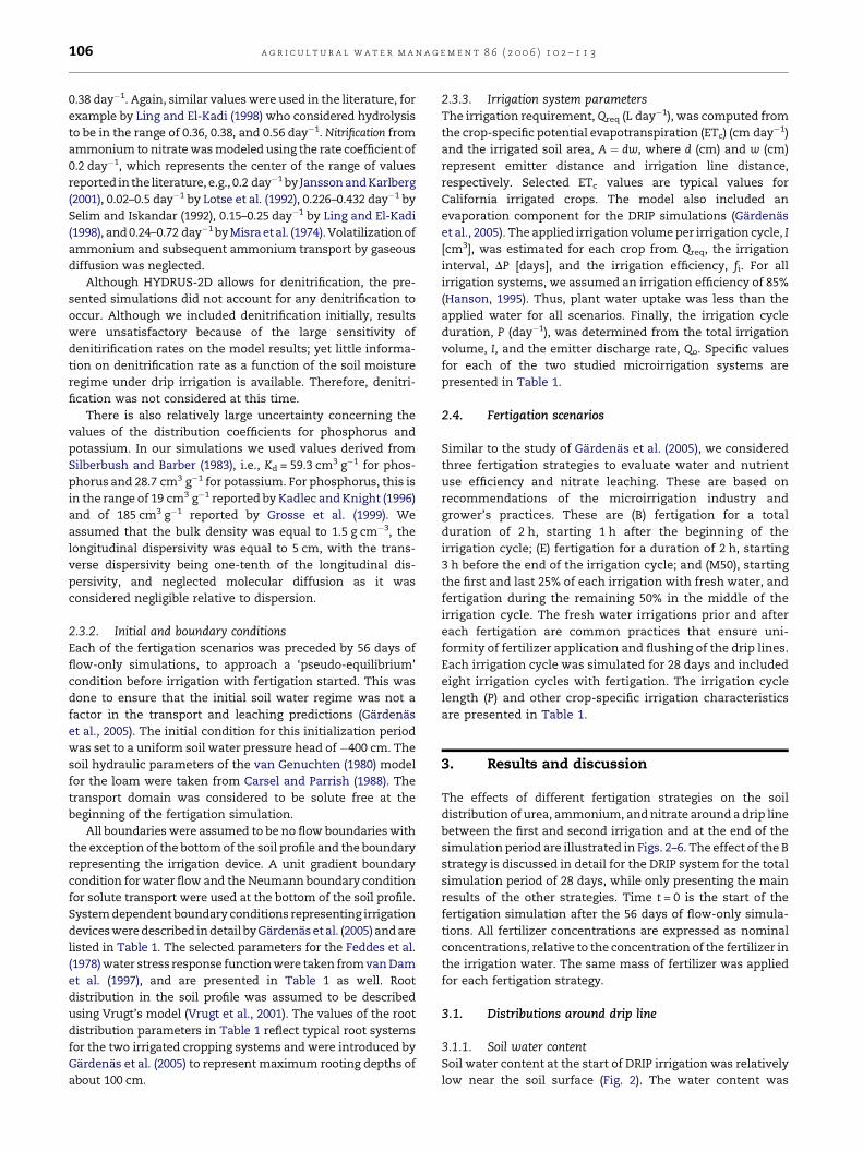
3.1.1. Soil water contentSoil water content at the start of DRIP irrigation was relatively
low near the soil surface (Fig. 2). The water content was
a g r i c u l t u r a l w a t e r m a n a g e m e n t 8 6 ( 2 0 0 6 ) 1 0 2 – 1 1 3 107
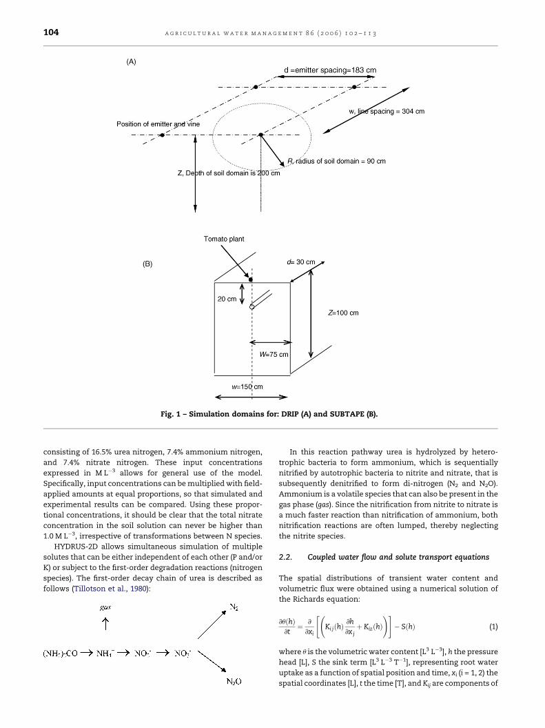
Fig. 2 – Volumetric soil water content distributions at the
start and conclusion of irrigation for DRIP and SUBTAPE
microirrigation systems.
maximum between the 60 and 140 cm soil depth, and was
controlled by root water uptake. After each irrigation, the
wetted region exhibited a vertically elongated pattern and
extended to nearly 60 cm horizontally and 100 cm vertically
directly beneath the emitter. A zone of relatively wet soil
occurred near the surface between 40 and 60 cm from the drip
line. This distinct wetting front position is the combined result
of wetting front advance during irrigation and a decreased root
distribution density away from the drip line.
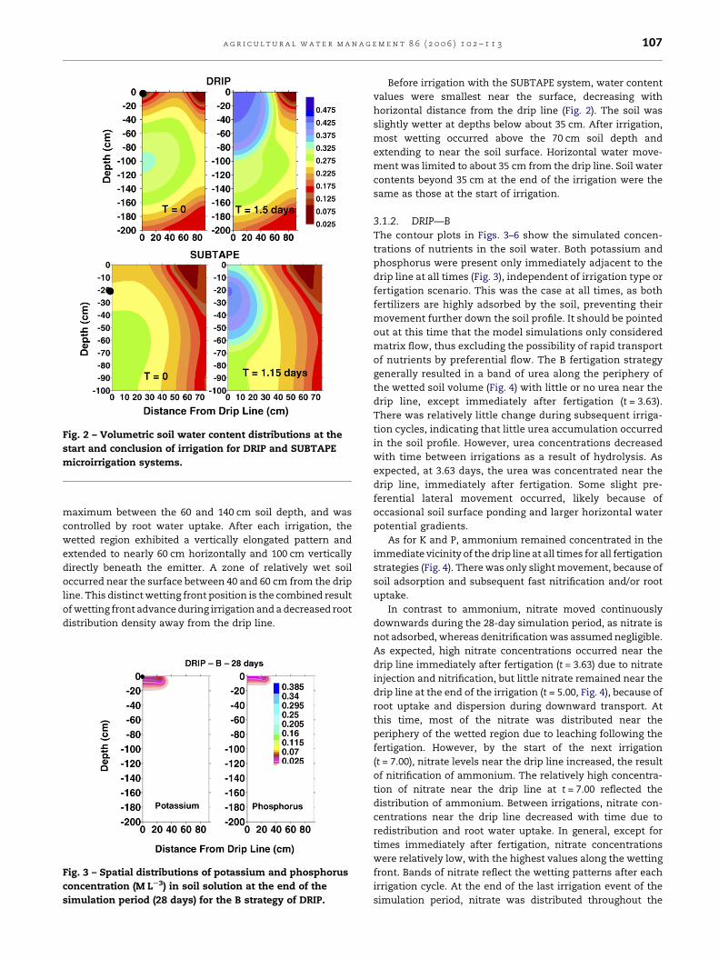
Fig. 3 – Spatial distributions of potassium and phosphorus
concentration (M LS3) in soil solution at the end of the
simulation period (28 days) for the B strategy of DRIP.
Before irrigation with the SUBTAPE system, water content
values were smallest near the surface, decreasing with
horizontal distance from the drip line (Fig. 2). The soil was
slightly wetter at depths below about 35 cm. After irrigation,
most wetting occurred above the 70 cm soil depth and
extending to near the soil surface. Horizontal water move-
ment was limited to about 35 cm from the drip line. Soil water
contents beyond 35 cm at the end of the irrigation were the
same as those at the start of irrigation.
3.1.2. DRIP—BThe contour plots in Figs. 3–6 show the simulated concen-
trations of nutrients in the soil water. Both potassium and
phosphorus were present only immediately adjacent to the
drip line at all times (Fig. 3), independent of irrigation type or
fertigation scenario. This was the case at all times, as both
fertilizers are highly adsorbed by the soil, preventing their
movement further down the soil profile. It should be pointed
out at this time that the model simulations only considered
matrix flow, thus excluding the possibility of rapid transport
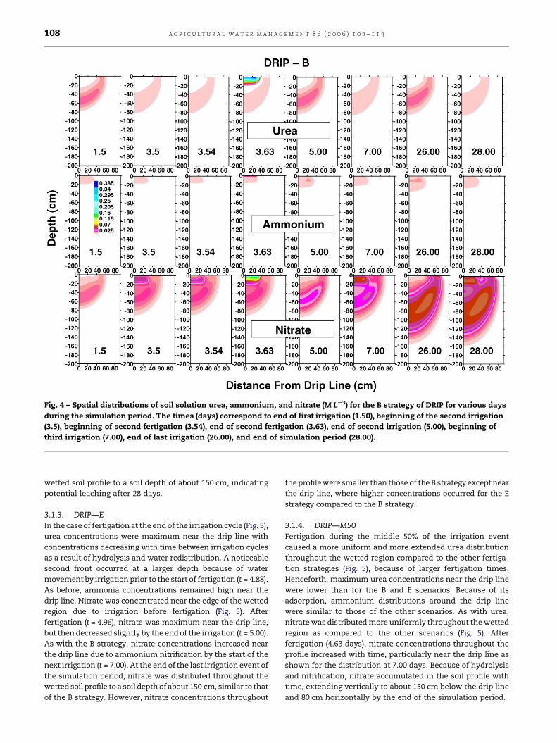
of nutrients by preferential flow. The B fertigation strategy
generally resulted in a band of urea along the periphery of
the wetted soil volume (Fig. 4) with little or no urea near the
drip line, except immediately after fertigation (t = 3.63).
There was relatively little change during subsequent irriga-
tion cycles, indicating that little urea accumulation occurred
in the soil profile. However, urea concentrations decreased
with time between irrigations as a result of hydrolysis. As
expected, at 3.63 days, the urea was concentrated near the
drip line, immediately after fertigation. Some slight pre-
ferential lateral movement occurred, likely because of
occasional soil surface ponding and larger horizontal water
potential gradients.
As for K and P, ammonium remained concentrated in the
immediate vicinity of the drip line at all times for all fertigation
strategies (Fig. 4). There was only slight movement, because of
soil adsorption and subsequent fast nitrification and/or root
uptake.
In contrast to ammonium, nitrate moved continuously
downwards during the 28-day simulation period, as nitrate is
not adsorbed, whereas denitrification was assumed negligible.
As expected, high nitrate concentrations occurred near the
drip line immediately after fertigation (t = 3.63) due to nitrate
injection and nitrification, but little nitrate remained near the
drip line at the end of the irrigation (t = 5.00, Fig. 4), because of
root uptake and dispersion during downward transport. At
this time, most of the nitrate was distributed near the
periphery of the wetted region due to leaching following the
fertigation. However, by the start of the next irrigation
(t = 7.00), nitrate levels near the drip line increased, the result
of nitrification of ammonium. The relatively high concentra-
tion of nitrate near the drip line at t = 7.00 reflected the
distribution of ammonium. Between irrigations, nitrate con-
centrations near the drip line decreased with time due to
redistribution and root water uptake. In general, except for
times immediately after fertigation, nitrate concentrations
were relatively low, with the highest values along the wetting
front. Bands of nitrate reflect the wetting patterns after each
irrigation cycle. At the end of the last irrigation event of the
simulation period, nitrate was distributed throughout the
a g r i c u l t u r a l w a t e r m a n a g e m e n t 8 6 ( 2 0 0 6 ) 1 0 2 – 1 1 3108
Fig. 4 – Spatial distributions of soil solution urea, ammonium, and nitrate (M LS3) for the B strategy of DRIP for various days
during the simulation period. The times (days) correspond to end of first irrigation (1.50), beginning of the second irrigation
(3.5), beginning of second fertigation (3.54), end of second fertigation (3.63), end of second irrigation (5.00), beginning of
third irrigation (7.00), end of last irrigation (26.00), and end of simulation period (28.00).
wetted soil profile to a soil depth of about 150 cm, indicating
potential leaching after 28 days.
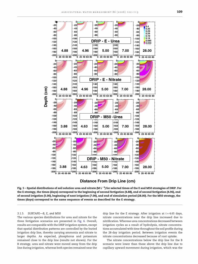
3.1.3. DRIP—EIn the case of fertigation at the end of the irrigation cycle (Fig. 5),
urea concentrations were maximum near the drip line with
concentrations decreasing with time between irrigation cycles
as a result of hydrolysis and water redistribution. A noticeable
second front occurred at a larger depth because of water
movement by irrigation prior to the start of fertigation (t = 4.88).
As before, ammonia concentrations remained high near the
drip line. Nitrate was concentrated near the edge of the wetted
region due to irrigation before fertigation (Fig. 5). After
fertigation (t = 4.96), nitrate was maximum near the drip line,
but then decreased slightly by the end of the irrigation (t = 5.00).
As with the B strategy, nitrate concentrations increased near
the drip line due to ammonium nitrification by the start of the
next irrigation (t = 7.00). At the end of the last irrigation event of
the simulation period, nitrate was distributed throughout the
wetted soil profile to a soil depth of about 150 cm, similar to that
of the B strategy. However, nitrate concentrations throughout
the profile were smaller than those of the B strategy except near
the drip line, where higher concentrations occurred for the E
strategy compared to the B strategy.
3.1.4. DRIP—M50Fertigation during the middle 50% of the irrigation event
caused a more uniform and more extended urea distribution
throughout the wetted region compared to the other fertiga-
tion strategies (Fig. 5), because of larger fertigation times.
Henceforth, maximum urea concentrations near the drip line
were lower than for the B and E scenarios. Because of its
adsorption, ammonium distributions around the drip line
were similar to those of the other scenarios. As with urea,
nitrate was distributed more uniformly throughout the wetted
region as compared to the other scenarios (Fig. 5). After
fertigation (4.63 days), nitrate concentrations throughout the
profile increased with time, particularly near the drip line as
shown for the distribution at 7.00 days. Because of hydrolysis
and nitrification, nitrate accumulated in the soil profile with
time, extending vertically to about 150 cm below the drip line
and 80 cm horizontally by the end of the simulation period.
a g r i c u l t u r a l w a t e r m a n a g e m e n t 8 6 ( 2 0 0 6 ) 1 0 2 – 1 1 3 109
Fig. 5 – Spatial distributions of soil solution urea and nitrate (M LS3) for selected times of the E and M50 strategies of DRIP. For
the E strategy, the times (days) correspond to the beginning of second fertigation (4.88), end of second fertigation (4.96), end
of second irrigation (5.00), beginning of next irrigation (7.00), and end of simulation period (28.00). For the M50 strategy, the
times (days) correspond to the same sequence of events as described for the E strategy.
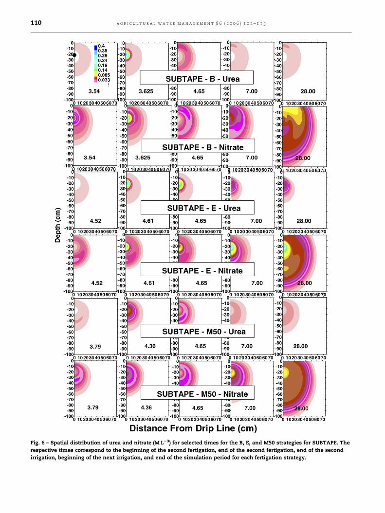
3.1.5. SUBTAPE—B, E, and M50The various species distributions for urea and nitrate for the
three fertigation scenarios are presented in Fig. 6. Overall,
results are comparable with the DRIP irrigation system, except
that spatial distribution patterns are controlled by the buried
irrigation drip line, thereby carrying ammonia and nitrate to
larger depths. As expected, phosphorus and potassium
remained close to the drip line (results not shown). For the
B strategy, urea and nitrate were moved away from the drip
line during irrigation, whereas both species remained near the
drip line for the E strategy. After irrigation at t = 4.65 days,
nitrate concentrations near the drip line increased due to
nitrification. Whereas urea concentrations decreased between
irrigation cycles as a result of hydrolysis, nitrate concentra-
tions accumulated with time throughout the soil profile during
the 28-day irrigation period. Between irrigation events the
nitrate concentrations decreased because of root uptake.
The nitrate concentrations below the drip line for the B
scenario were lower than those above the drip line due to
capillary upward movement during irrigation, which was the
a g r i c u l t u r a l w a t e r m a n a g e m e n t 8 6 ( 2 0 0 6 ) 1 0 2 – 1 1 3110
Fig. 6 – Spatial distribution of urea and nitrate (M LS3) for selected times for the B, E, and M50 strategies for SUBTAPE. The
respective times correspond to the beginning of the second fertigation, end of the second fertigation, end of the second
irrigation, beginning of the next irrigation, and end of the simulation period for each fertigation strategy.
a g r i c u l t u r a l w a t e r m a n a g e m e n t 8 6 ( 2 0 0 6 ) 1 0 2 – 1 1 3 111
opposite for the E strategy. For the M50 strategy, nitrate was
distributed more uniformly throughout the wetted region as
compared to the B and E strategies (Fig. 6).
3.2. Mass balance
Since we used dimensional concentrations in our simulations,
the dimension of mass in the mass balance calculations are
either [M] for the axi-symmetric geometry of DRIP or [M cm�1]
for the two-dimensional geometry of SUBTAPE, and includes
the sorbed mass.
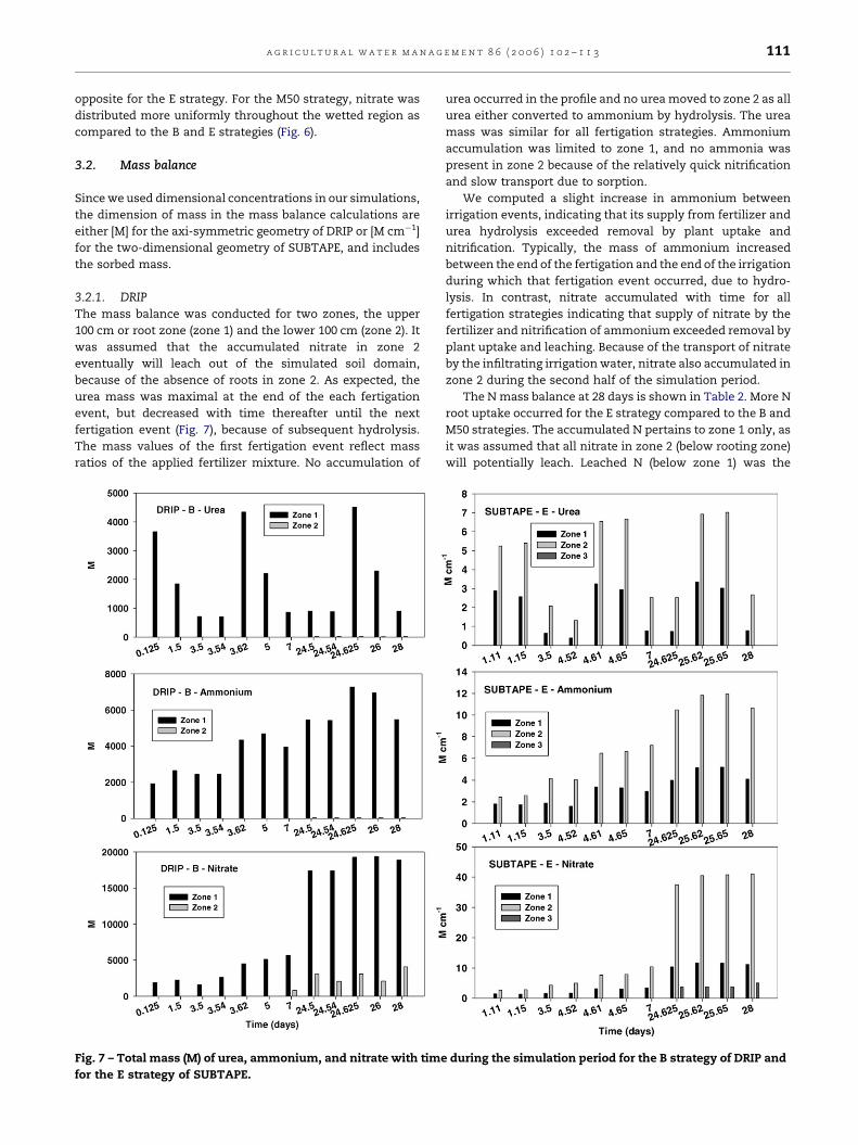
3.2.1. DRIPThe mass balance was conducted for two zones, the upper
100 cm or root zone (zone 1) and the lower 100 cm (zone 2). It
was assumed that the accumulated nitrate in zone 2
eventually will leach out of the simulated soil domain,
because of the absence of roots in zone 2. As expected, the
urea mass was maximal at the end of the each fertigation
event, but decreased with time thereafter until the next
fertigation event (Fig. 7), because of subsequent hydrolysis.
The mass values of the first fertigation event reflect mass
ratios of the applied fertilizer mixture. No accumulation of
Fig. 7 – Total mass (M) of urea, ammonium, and nitrate with time
for the E strategy of SUBTAPE.
urea occurred in the profile and no urea moved to zone 2 as all
urea either converted to ammonium by hydrolysis. The urea
mass was similar for all fertigation strategies. Ammonium
accumulation was limited to zone 1, and no ammonia was
present in zone 2 because of the relatively quick nitrification
and slow transport due to sorption.
We computed a slight increase in ammonium between
irrigation events, indicating that its supply from fertilizer and
urea hydrolysis exceeded removal by plant uptake and
nitrification. Typically, the mass of ammonium increased
between the end of the fertigation and the end of the irrigation
during which that fertigation event occurred, due to hydro-
lysis. In contrast, nitrate accumulated with time for all
fertigation strategies indicating that supply of nitrate by the
fertilizer and nitrification of ammonium exceeded removal by
plant uptake and leaching. Because of the transport of nitrate
by the infiltrating irrigation water, nitrate also accumulated in
zone 2 during the second half of the simulation period.
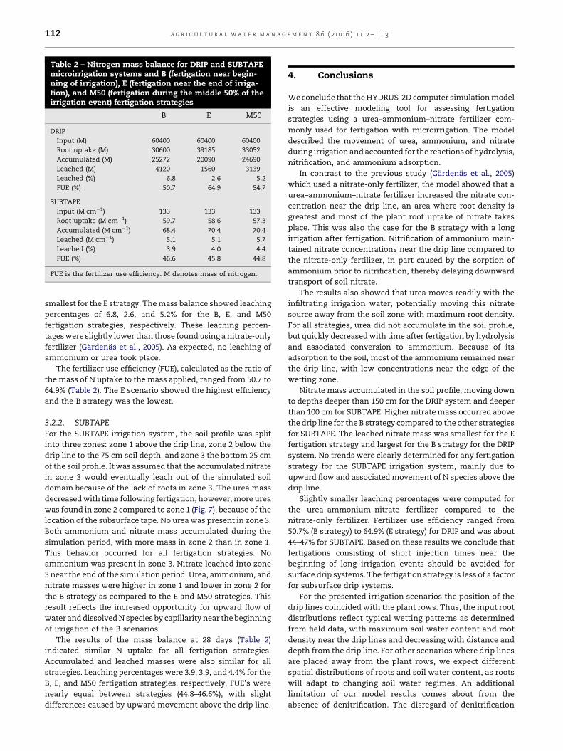
The N mass balance at 28 days is shown in Table 2. More N
root uptake occurred for the E strategy compared to the B and
M50 strategies. The accumulated N pertains to zone 1 only, as
it was assumed that all nitrate in zone 2 (below rooting zone)
will potentially leach. Leached N (below zone 1) was the
during the simulation period for the B strategy of DRIP and
a g r i c u l t u r a l w a t e r m a n a g e m e n t 8 6 ( 2 0 0 6 ) 1 0 2 – 1 1 3112
Table 2 – Nitrogen mass balance for DRIP and SUBTAPEmicroirrigation systems and B (fertigation near begin-ning of irrigation), E (fertigation near the end of irriga-tion), and M50 (fertigation during the middle 50% of theirrigation event) fertigation strategies
B E M50
DRIP
Input (M) 60400 60400 60400
Root uptake (M) 30600 39185 33052
Accumulated (M) 25272 20090 24690
Leached (M) 4120 1560 3139
Leached (%) 6.8 2.6 5.2
FUE (%) 50.7 64.9 54.7
SUBTAPE
Input (M cm�1) 133 133 133
Root uptake (M cm�1) 59.7 58.6 57.3
Accumulated (M cm�1) 68.4 70.4 70.4
Leached (M cm�1) 5.1 5.1 5.7
Leached (%) 3.9 4.0 4.4
FUE (%) 46.6 45.8 44.8
FUE is the fertilizer use efficiency. M denotes mass of nitrogen.
smallest for the E strategy. The mass balance showed leaching
percentages of 6.8, 2.6, and 5.2% for the B, E, and M50
fertigation strategies, respectively. These leaching percen-
tages were slightly lower than those found using a nitrate-only
fertilizer (Gardenas et al., 2005). As expected, no leaching of
ammonium or urea took place.
The fertilizer use efficiency (FUE), calculated as the ratio of
the mass of N uptake to the mass applied, ranged from 50.7 to
64.9% (Table 2). The E scenario showed the highest efficiency
and the B strategy was the lowest.
3.2.2. SUBTAPEFor the SUBTAPE irrigation system, the soil profile was split
into three zones: zone 1 above the drip line, zone 2 below the
drip line to the 75 cm soil depth, and zone 3 the bottom 25 cm
of the soil profile. It was assumed that the accumulated nitrate
in zone 3 would eventually leach out of the simulated soil
domain because of the lack of roots in zone 3. The urea mass
decreased with time following fertigation, however, more urea
was found in zone 2 compared to zone 1 (Fig. 7), because of the
location of the subsurface tape. No urea was present in zone 3.
Both ammonium and nitrate mass accumulated during the
simulation period, with more mass in zone 2 than in zone 1.
This behavior occurred for all fertigation strategies. No
ammonium was present in zone 3. Nitrate leached into zone
3 near the end of the simulation period. Urea, ammonium, and
nitrate masses were higher in zone 1 and lower in zone 2 for
the B strategy as compared to the E and M50 strategies. This
result reflects the increased opportunity for upward flow of
water and dissolved N species by capillarity near the beginning
of irrigation of the B scenarios.
The results of the mass balance at 28 days (Table 2)
indicated similar N uptake for all fertigation strategies.
Accumulated and leached masses were also similar for all
strategies. Leaching percentages were 3.9, 3.9, and 4.4% for the
B, E, and M50 fertigation strategies, respectively. FUE’s were
nearly equal between strategies (44.8–46.6%), with slight
differences caused by upward movement above the drip line.
4. Conclusions
We conclude that the HYDRUS-2D computer simulation model
is an effective modeling tool for assessing fertigation
strategies using a urea–ammonium–nitrate fertilizer com-
monly used for fertigation with microirrigation. The model
described the movement of urea, ammonium, and nitrate
during irrigation and accounted for the reactions of hydrolysis,
nitrification, and ammonium adsorption.
In contrast to the previous study (Gardenas et al., 2005)
which used a nitrate-only fertilizer, the model showed that a
urea–ammonium–nitrate fertilizer increased the nitrate con-
centration near the drip line, an area where root density is
greatest and most of the plant root uptake of nitrate takes
place. This was also the case for the B strategy with a long
irrigation after fertigation. Nitrification of ammonium main-
tained nitrate concentrations near the drip line compared to
the nitrate-only fertilizer, in part caused by the sorption of
ammonium prior to nitrification, thereby delaying downward
transport of soil nitrate.
The results also showed that urea moves readily with the
infiltrating irrigation water, potentially moving this nitrate
source away from the soil zone with maximum root density.
For all strategies, urea did not accumulate in the soil profile,
but quickly decreased with time after fertigation by hydrolysis
and associated conversion to ammonium. Because of its
adsorption to the soil, most of the ammonium remained near
the drip line, with low concentrations near the edge of the
wetting zone.
Nitrate mass accumulated in the soil profile, moving down
to depths deeper than 150 cm for the DRIP system and deeper
than 100 cm for SUBTAPE. Higher nitrate mass occurred above
the drip line for the B strategy compared to the other strategies
for SUBTAPE. The leached nitrate mass was smallest for the E
fertigation strategy and largest for the B strategy for the DRIP
system. No trends were clearly determined for any fertigation
strategy for the SUBTAPE irrigation system, mainly due to
upward flow and associated movement of N species above the
drip line.
Slightly smaller leaching percentages were computed for
the urea–ammonium–nitrate fertilizer compared to the
nitrate-only fertilizer. Fertilizer use efficiency ranged from
50.7% (B strategy) to 64.9% (E strategy) for DRIP and was about
44–47% for SUBTAPE. Based on these results we conclude that
fertigations consisting of short injection times near the
beginning of long irrigation events should be avoided for
surface drip systems. The fertigation strategy is less of a factor
for subsurface drip systems.
For the presented irrigation scenarios the position of the
drip lines coincided with the plant rows. Thus, the input root
distributions reflect typical wetting patterns as determined
from field data, with maximum soil water content and root
density near the drip lines and decreasing with distance and
depth from the drip line. For other scenarios where drip lines
are placed away from the plant rows, we expect different
spatial distributions of roots and soil water content, as roots
will adapt to changing soil water regimes. An additional
limitation of our model results comes about from the
absence of denitrification. The disregard of denitrification
a g r i c u l t u r a l w a t e r m a n a g e m e n t 8 6 ( 2 0 0 6 ) 1 0 2 – 1 1 3 113
was intentional as there is no information available on
denitrification rates for soil moisture regimes under micro-
irrigation. Nevertheless, our simulation results provide
guidance on the appropriate fertigation strategy for many
typical microirrigation scenarios.
Acknowledgement
We acknowledge funding by the California FREP, Fertilizer
Research and Education Program.
r e f e r e n c e s
Bar-Yosef, B., 1999. Advances in fertigation. Adv. Agron. 65, 1–75.
Bassoi, L.H., Hopmans, J.W., de, L.A., Jorge, C., De Alencar, C.M.,Silva, J.A.M.E., 2003. Grapevine root distribution in drip andmicrosprinkler irrigation using monolith and the soil profilemethod. Scientia Agricola 60 (2), 377–387.
Carsel, R.F., Parrish, R.S., 1988. Developing joint probabilitydistributions of soil water retention characteristics. WaterResour. Res. 24, 755–769.
Cote, C.M., Bristow, K.L., Charlesworth, P.B., Cook, F.J., Thorburn,P.J., 2003. Analysis of soil wetting and solute transport insubsurface trickle irrigation. Irrig. Sci. 22, 143–156.
Feddes, R.A., Kowalik, P.J., Zaradny, H., 1978. Simulation of fieldwater use and crop yield. In: Simulation Monographs,Pudoc, Wageningen.
Gardenas, A., Hopmans, J.W., Hanson, B.R., Simunek, J., 2005.Two-dimensional modeling of nitrate leaching for differentfertigation strategies under micro-irrigation. Agric. WaterManage. 74, 219–242.
Grosse, W., Wissing, F., Perfler, R., Wu, Z., Chang, J., Lei, Z., 1999.Biotechnological approach to water quality improvement intropical and subtropical areas for reuse and rehabilitation ofaquatic ecosystems. Final report, INCO-DC Project ContractNo. ERBIC18CT960059. Cologne, Germany.
Hansen, S., Jensen, H.E., Nielsen, N.E., Svendsen, H., 1990.DAISY: Soil Plant Atmosphere System Model. NPO ReportNo. A 10. The National Agency for EnvironmentalProtection, Copenhagen, 272 pp.
Hanson, B.R., 1995. Practical potential irrigation efficiencies. In:Water Resources Engineering: Proceedings of the FirstInternational Conference. The American Society of CivilEngineers, San Antonio, TX, August 14–18.
Heinen, M., 2001. FUSSIM2: brief description of the simulationmodel and application to fertigation scenarios. Agronomie21, 285–296.
Hopmans, J.W., Bristow, K.L., 2002. Current capabilities andfuture needs of rooot water and nutirent uptake modeling.Adv. Agron. 77, 104–175.
Hutson, J.L., Wagenet, R.J., 1991. Simulating nitrogen dynamics insoils using a deterministic model. Soil Use Manage. 7, 74–78.
Jansson, P.-E., Karlberg, L., 2001. Coupled Heat and MassTransfer Model for Soil–Plant–Atmosphere systems. RoyalInstitute of Technology, Department of Civil andEnvironmental Engineering, Stockholm, 325 pp.
Silberbush, M., Barber, S.A., 1983. Prediction of phosphorus andpotassium uptake by soybeans with a mechanisticmathematical model. Soil Sci. Soc. Am. J. 47, 262–265.
Simunek, J., Sejna, M., Van Genuchten, M.Th., 1999. TheHYDRUS-2D software package for simulating two-dimensonal movement of water, heat, and multiple solutesin variable saturated media. Version 2.0, IGWMC-TPS-53.International Ground Water Modeling Center, ColoradoSchool of Mines, Golden, Colorado.
Somma, F., Clausnitzer, V., Hopmans, J.W., 1998. Modeling oftransient three-dimensional soil water and solute transportwith root growth and water and nutrient uptake. Plant Soil202, 281–293.
Tanji, K.K., Mehran, M., Gupta, S.K., 1981. Water and nitrogenfluxes in the root zone of irrigated maize. In: Frissel, M.J.,van Veen, J.A. (Eds.), Simulation of Nitrogen Behavior ofSol–Plant Systems. PUDOC, Wageningen, the Netherlands,pp. 51–67.
van Dam, J.C., Huygen, J., Wesseling, J.G., Feddes, R.A., Kabat, P.,van Valsum, P.E.V., Groenendijk, P., van Diepen, C.A., 1997.Theory of SWAP, Version 2.0. Simulation of water flow,solute transport and plant growth in the Soil- Water-Atmosphere- Plant environment. Department of WaterResources, WAU, Report 71, DLO Winand Staring Centre,Wageningen, Technical Document 45.
van Genuchten, M.Th., 1980. A closed-form equation forpredicting the hydraulic conductivity of unsaturated soils.Soil Sci. Soc. Am. J. 44, 892–1037.
Vrugt, J.A., Hopmans, J.W., Simunek, J., 2001. Calibration of atwo-dimensional root water uptake. Soil Sci. Soc. Am. J. 65,1027–1037.
Wagenet, R.J., Biggar, J.W., Nielsen, D.R., 1977. Tracing thetransformation of urea fertilizer during leaching. Soil Sci.Soc. Am. J 41, 896–902.
Weinbaum, S.A., Johnson, R.S., Dejong, T.M., 1992. Causes andconsequences of overfertilization in orchards. Proceedingsof the Workshop Fertilizer Management in HorticulturalCrops: Implications for Water Pollution, Hort. Technol. 2,112–120.