Numerical Modelling of Heat and Mass Transfer and Optimisation of a Natural Draft Wet Cooling Tower By N.J.Williamson A Dissertation Submitted to the School of Aerospace, Mechanical and Mechatronic Engineering The University of Sydney in Fulfilment of the Requirements for the Degree of Doctor of Philosophy Copyright c N.J. Williamson 2008 All rights reserved
Transcript
Numerical Modelling of
Heat and Mass Transfer
and Optimisation of a
Natural Draft Wet Cooling
Tower
By
N.J.Williamson
A Dissertation Submitted to
the School of Aerospace, Mechanical and Mechatronic
The better predictions of the centreline velocity on mesh B by the DRM
model appears to be a result of too much dissipation in the region, y+ < 70.
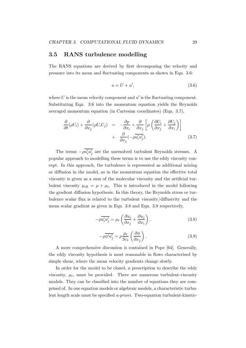
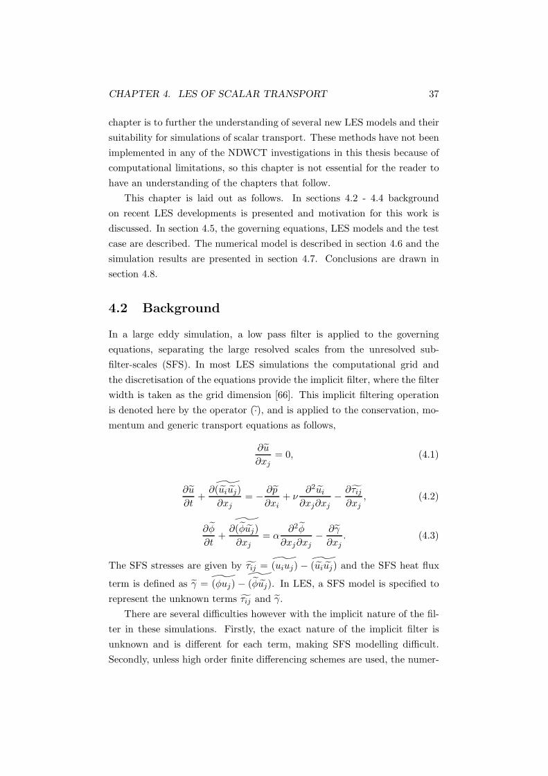
The mean temperature profile is given in Fig. 4.3, non-dimensionalised
by wall friction temperature, 〈φ+〉 = 〈φ〉/Tτ where Tτ = qw/ρcpuτ . Exam-
ining the figure, it is clear the source of the poor results for the Nusselt
number. The centreline temperature is very poorly predicted by all models.
The DRM model captures the behaviour fairly well for y+ < 80 but gives
the worst prediction of the centreline temperature. This follows directly
from the predictions of the velocity profile. The profiles are worse on mesh
B but because of the additional dissipation, the centreline temperature ac-
tually gets closer to the DNS result. None of the models predict the rise in
temperature at the channel centre well.
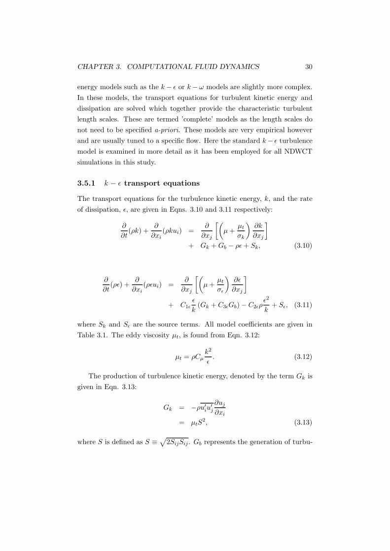
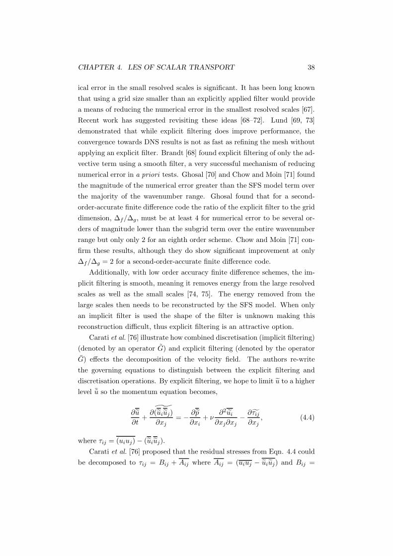
The shear stress 〈u′v′〉 is shown in Fig. 4.4 (a). This is calculated as
Ruv = −〈u′v′〉 − 〈τxy〉, where u′ is the fluctuating resolved velocity compo-
nent calculated using, u = 〈u〉 + u′ and τxy is the model component. The
shear stress is predicted by all models, with clear improvements over the no-
model case. Both the DMM and DRM models perform better than the DSM
in the buffer layer region for y+ < 20, but over predict the peak slightly.
The model component for of the shear stress, τxy, is shown in Fig. 4.4 (b). It
is much greater for both the DMM and the DRM. This is expected because
the explicit filtering means that the model represents a greater part of the
spectrum.
The traceless normal stresses R∗
xx,R∗
yy and R∗
zz, are compared in Fig.
4.5. They are calculated as, −Rxx = 〈u′u′〉 − 〈τxx〉. The trace is subtracted
following, R∗
xx = Rxx − 1/3(Rxx + Ryy + Rzz). This is important because
CHAPTER 4. LES OF SCALAR TRANSPORT 52
1 10 100y
+
0
5
10
15
20
25
< θ
+ >
no model DSMDMMDRMDNS
(a)
1 10 100y
+
0
5
10
15
20
25
< θ
+ >
DSMDMM_DSMDRMDRM_DSMDNS
(b)
1 10 100y
+
0
5
10
15
20
25
< θ
+ >
DSMDMMDRMDRM (mesh A)DNS
(c)
Figure 4.3: Mean temperature profile in wall units for mesh A (a-b) andmesh B (c)
CHAPTER 4. LES OF SCALAR TRANSPORT 53
1 10 100y
+
0
0.2
0.4
0.6
0.8
1
Rxy
/uτ2
no modelDSMDMMDRMDNS
(a)
0 25 50 75 100 125 150y
+
0
0.1
0.2
< τ
xy >
/ uτ2
DSMDMMDRM
(b)
Figure 4.4: Total Reynolds stress Rxy for mesh A (a) and model subgridscale shear stress τxy for mesh A (b)
CHAPTER 4. LES OF SCALAR TRANSPORT 54
the dynamic Smagorinsky component of the models, provides no model for
the trace and thus the normal stresses cannot be compared directly with
DNS results unless the trace is removed [79]. It is also important to include
the model component, as this can be very significant in the models with the
τRSFS term such as the DRM or DMM. Gullbrand and Chow [80] did not
include the model component in their comparison and came to the conclusion
that the normal stresses were dramatically better predicted by the DMM
and DRM model. In fact, the resolved component is simply reduced in
these models as the SFS model contributes more. Including the effect of the
subgrid model as in Fig. 4.5, shows that the normal stresses are predicted
the same by all models, with only slightly poorer results with the DSM.
The scalar flux from the walls hy, is calculated using hy = 〈v′φ′〉/uτTτ +
〈γy〉/uτTτ . The results for mesh A and mesh B are given in Fig. 4.6 (a-b)
and Fig. 4.6 (c) respectively. The model component is given in Fig. 4.7.
Again, the DSM and no model cases perform poorly compared with the
DMM and DRM models, which capture the behaviour in the buffer region
(y+ ∼ 5−20) better. The model component γy behaves in a similar manner
to τxy, with its value much lower in DSM simulation than with the DRM
and DMM models.
The effect of scalar subgrid heat flux model was examined more closely by
using the DMM and DRM models for τ and using the DSM model for γ. In
this way the velocity field is explicitly filtered but the scalar field is not. This
means there is an inconsistency in the application of the filters and so this
method cannot be recommended. It does however give some indication of
how the models are working. In Fig. 4.3 (b), the mean temperature profiles
for the DRM/DSM and DMM/DSM models are given. In both cases, the
DMM/DSM and DRM/DSM results move closer to those of the DSM and
away from the DMM or DRM predictions. On Fig. 4.6, hy predicted by the
DRM/DSM is again between the DSM and DRM profiles. The DRM/DSM
combination does not predict hy in the buffer region (y+ ∼ 5 − 20) as well
as the DRM model on both mesh A and mesh B. This does suggest that the
reconstruction terms are important for both γ and τ .
The flow statistics for the DRM model in this study are similar to those
of Gullbrand and Chow [80], at Reτ = 395. In that study however, the
predictions of the mean streamwise velocity in the channel centre were no
worse than the predictions throughout the log-law region. In this study,
CHAPTER 4. LES OF SCALAR TRANSPORT 55
1 10 100
y+
-5
-4
-3
-2
-1
0
Rxx
*/u τ2
no modelDSMDMMDRMDNS
1 10 100
y+
0
0.5
1
1.5
2
2.5
3
Ryy
*/u τ2
1 10 100
y+
0
0.5
1
1.5
2
2.5
3
Rzz
*/u τ2
Figure 4.5: Traceless Reynolds stress on mesh A
CHAPTER 4. LES OF SCALAR TRANSPORT 56
1 10 100y
+
-1
-0.8
-0.6
-0.4
-0.2
0
h y
no modelDSMDMMDRMDNS
(a)
1 10 100y
+
-1
-0.8
-0.6
-0.4
-0.2
0
h y
DSMDRMDRM_DSMDNS
(b)
1 10 100y
+
-1
-0.8
-0.6
-0.4
-0.2
0
h y
DSMDMMDRMDRM_DSMDNS
(c)
Figure 4.6: Resolved and modelled temperature flux, hy = 〈v′φ′〉/uτTτ +〈γy〉/uτTτ on mesh A (a) and (b) and mesh B (c)
CHAPTER 4. LES OF SCALAR TRANSPORT 57
1 10 100
y+
-0.2
-0.15
-0.1
-0.05
0
< γ
y >/ (
uτT
τ)
DSMDMMDRM
Figure 4.7: Model subgrid heat flux hy for mesh A
the DRM better captures the velocity through the log-law region and the
buffer region than the DMM and DSM models, but it performs poorly in the
centre of the channel. In mesh A, the maximum cell dimension in the wall
normal direction is ∆y+ = 8.7. This should be sufficient for LES. The better
results of Gullbrand and Chow [80] suggest that the poor predictions of the
centre-line velocity may be a low Reynolds number effect. In the present
study with Reτ = 150, the log-law region is quite small (y+ ∼ 20−80). The
models in this study may not perform as well at low Reynolds numbers.
This may be due to the dynamic Smagorinsky term in the models. In the
less turbulent flow considered here, similarity between the test filtered level
( ˆG) and the G level, may not be as strong, possibly leading to an under
prediction of the model dissipation at the centre of the channel.
There is predictably a strong correlation between the predictions of the
scalar temperature profile and the mean velocity profile. The poor perfor-
mance of all the models at predicting the mean temperature profile, does
not necessarily mean that the models are inadequate for modelling γ. Both
the velocity field and the scalar SFS model determine the transport of φ.
The temperature profile appears to be more difficult to capture accurately
than the velocity profile. The sharp rise in temperature in the centre of the
channel which is seen in the DNS result, is not captured in any of the LES
simulations. This may again be a low Reynolds number effect which needs
to be tested.
CHAPTER 4. LES OF SCALAR TRANSPORT 58
4.8 Conclusions
Several large eddy simulation models have been examined within the frame-
work of explicit filtering and reconstruction outlined by Carati et al. [76].
The DMM and DRM models have been applied to the simulation of trans-
port of a passive scalar in a turbulent channel flow. Compared with the
DSM model and no-model, where no reconstruction is performed, the DMM
and DRM models perform quite well.
For the prediction of the turbulent stresses and the mean flow statistics,
all the models perform better than the ’no-model’ simulation. Both the
DMM and the DRM perform better than the DSM for most of the quantities
examined, particularly in the buffer region and through most of the log-law
region. The DRM model appears to offer some improvement over the DMM,
but overall the results are mixed. The DRM underpredicts the mean velocity
in the centre of the channel.
The results for the transport of a passive scalar are less successful. None
of the models predicted the correct mean temperature profile across the
channel. The DRM seems slightly better in the region close to the wall, but
underpredicts the temperature in the centre of the channel more severely
than the other models. The Nusselt numbers were similarly poorly pre-
dicted. The scalar flux from the wall was quite well predicted by the DRM
and DMM for y+ < 40. The no-model and DSM models performed more
poorly here. In the centre of the channel, the flux was over predicted by all
models.
Overall, it appears that the DRM and DMM are promising concepts, for
modelling both the scalar SGS model and the residual stress. For most of the
statistics examined, both models perform better than the DSM model. In
several of the statistics examined however, their performance was mixed, so
more work is needed before they can be trusted in more difficult simulations.
Further tests are needed at higher Reynolds number to confirm these results.
Having performed these calculations it is interesting to relate them back
to the simulation of a NDWCT. The computational cost or simulation time
of LES increases with the Reynolds number simulated. The scaling goes
like ∼ Re3. In this study, turbulent channel flow at Re = 4560 has been
examined. The Reynolds number for an entire NDWCT is ∼ 1.7 × 10⁷,
approximately 4×10³ times higher than that for the channel flow simulation.
CHAPTER 4. LES OF SCALAR TRANSPORT 59
Thus the computational time ∼ 5 × 10¹⁰ longer. With simulations in this
study taking approximately 40 hours in a single processor, this means a
similarly well resolved LES simulation of the entire cooling tower would
take in the order of 200 million years. Thus full tower modelling with well
resolved LES is completely unrealistic on modern computers. LES may be
able to be applied in some isolated small regions of the tower however, such
as an isolated small section of the fill.
Chapter 5
Two Dimensional
Axisymmetric NDWCT
Model
5.1 Introduction
In this chapter, a numerical model of a NDWCT is presented with its vali-
dation against manufacturers’ performance curves. In sections 5.2 to 5.10,
the detail of the heat and mass transfer calculations are presented and the
fill modelling approach validated. The overall model is validated in section
5.10 and in section 5.11 results are presented. More detailed analysis of the
results and a parametric study is contained in Chapter 6.
5.2 Model description
The numerical model has been built within FLUENT version 6.1 [40]. This
study only examines the flow in the tower under no-cross wind conditions, so
the mean flow should be two dimensional. Here a two-dimensional axisym-
metric model has been developed, as a full three dimensional model would
be too computationally expensive. The air/water flow in the tower has been
modelled using a two phase simulation. The gas phase (continuous phase)
has been modelled in Eulerian form as a mixture of air/water-vapour/water-
condensate. The second phase is the discrete water droplets in the spray
and rain zones. The droplets have been modelled using Lagrangian particle
60
CHAPTER 5. TWO DIMENSIONAL NDWCT MODEL 61
tracking in FLUENT, and this component is referred to as the discrete phase
model (DPM). The governing equations for incompressible steady air flow
can be written in general form as:
∇ · (ρuφ − Γφ∇φ) = Sφ, (5.1)
as given in Chapter 3. The flow properties of the Eulerian mixture compo-
nents and the DPM are given in Appendix B.
The very large range of scales in a NDWCT mean that it is impossible to
computationally represent all components of the tower numerically. Instead
the components that cannot appear directly in the model are represented
through source terms in Eqn. 5.1. The manner in which these source terms
are calculated and coupled with the continuous phase is detailed in the
following sections. The modelling of the drift eliminators, tower supports
and other features causing flow resistance is discussed in section 5.5. The
modelling of the air and water flow and the heat and mass transfer in the
fill is presented in section 5.7.
5.3 Domain and boundary conditions
The cooling tower geometry and specifications are based on a NDWCT
located at Mt. Piper Power Station (Delta Electricity), NSW, Australia;
designed by Hamon-Sobelco LTD, South Africa. This is a coal fired power
plant operating 2x660MW Units. Each unit is cooled by a NDWCT. The two
NDWCTs at this site have a history of underperforming, primarily due to
wind effects. The plant operators have been actively involved in a research
program to improve the performance of the NDWCTS [21, 36, 37]. The
towers at this site were chosen as the basis for this study as they are both
of a typical NDWCT design and the design and operating data were readily
available. The design parameters are given in Table 5.1 together with the
reference conditions used in this study. The performance curves from this
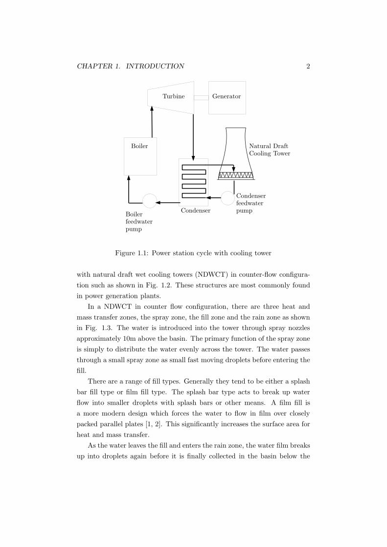
tower are used for the validation of the model.
The axisymmetric representation of the domain in this study is shown
in Fig. 5.1. In the reference tower, a 2.8m wide causeway runs through the
centre of the tower. This has been represented by a 1.4m wide blockage in
the axisymmetric model (see Fig. 5.1). The computational domain extends
CHAPTER 5. TWO DIMENSIONAL NDWCT MODEL 62
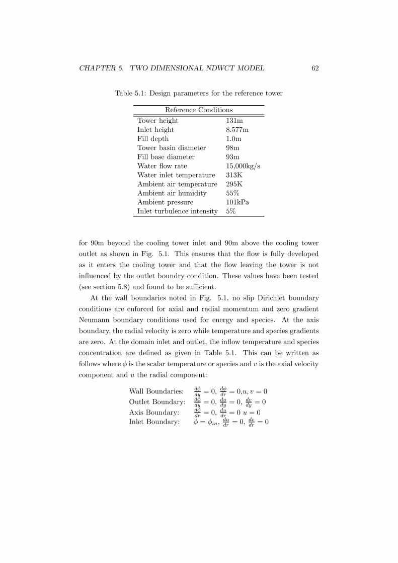
Table 5.1: Design parameters for the reference tower
Reference Conditions
Tower height 131mInlet height 8.577mFill depth 1.0mTower basin diameter 98mFill base diameter 93mWater flow rate 15,000kg/sWater inlet temperature 313KAmbient air temperature 295KAmbient air humidity 55%Ambient pressure 101kPaInlet turbulence intensity 5%
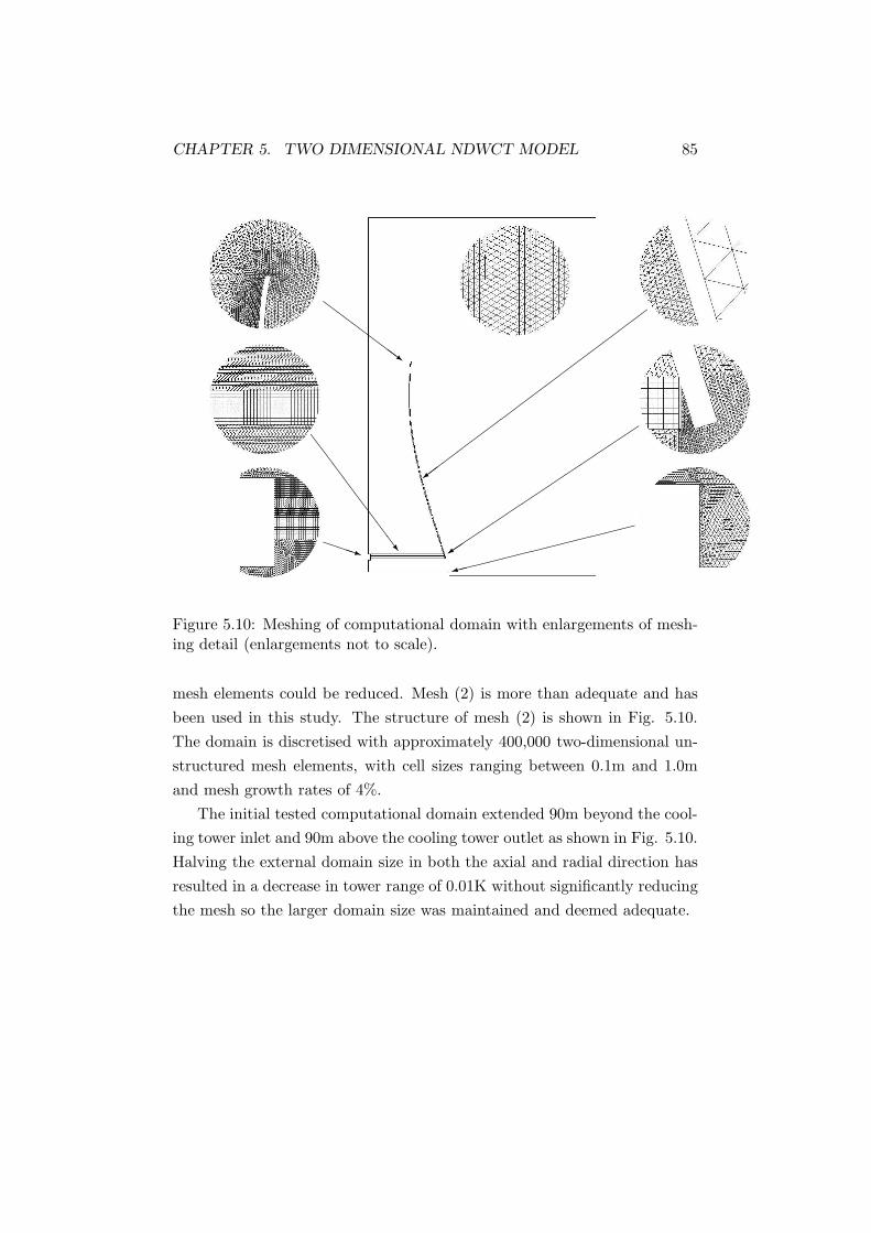
for 90m beyond the cooling tower inlet and 90m above the cooling tower
outlet as shown in Fig. 5.1. This ensures that the flow is fully developed
as it enters the cooling tower and that the flow leaving the tower is not
influenced by the outlet boundry condition. These values have been tested
(see section 5.8) and found to be sufficient.
At the wall boundaries noted in Fig. 5.1, no slip Dirichlet boundary
conditions are enforced for axial and radial momentum and zero gradient
Neumann boundary conditions used for energy and species. At the axis
boundary, the radial velocity is zero while temperature and species gradients
are zero. At the domain inlet and outlet, the inflow temperature and species
concentration are defined as given in Table 5.1. This can be written as
follows where φ is the scalar temperature or species and v is the axial velocity
component and u the radial component:
Wall Boundaries: dφdy = 0, dφ
dr = 0,u, v = 0
Outlet Boundary: dφdy = 0, du
dy = 0, dvdy = 0
Axis Boundary: dφdr = 0, du
dr = 0 u = 0
Inlet Boundary: φ = φin, dudr = 0, dv
dr = 0
CHAPTER 5. TWO DIMENSIONAL NDWCT MODEL 63
1 2 3456 InletHeight6?Ground WallInlet
OutletAxis ShellWall Rain ZoneSpray ZoneFill Zone �� �����������������������������
1
Figure 5.1: Computational domain (left) with heat and mass transfer regiondetail enlarged on right: (1) drift eliminators, (2) spray nozzles, (3) fill waterinlet (or fill air outlet), (4) fill water outlet (or fill air inlet), (5) basin, (6)causeway.
5.4 Solution procedure
An overview of the heat and mass transfer procedure and water flow repre-
sentation is as follows:
1. The water enters the tower through the spray nozzles. The water mass
flow rate and temperature are specified and droplet spray trajectories
are initiated at approximate nozzle locations across the tower (see
section 5.6.4).
2. The spray droplets pass through the spray zone (see Fig. 5.1) and
upon reaching the top surface of the fill, they are terminated and their
temperature is recorded and used as an input to the fill model.
3. In the fill an external procedure is used to determine the change in wa-
ter temperature and mass through the fill (section 5.7). This procedure
is implemented in subroutines, written in ’C’ programing language
and compiled directly into FLUENT through its USER-DEFINED-
FUNCTION (UDF) capabilities. The same procedure then calculates
the energy and mass source terms to couple the energy and mass trans-
fer with the continuous phase. Additionally, the procedure determines
CHAPTER 5. TWO DIMENSIONAL NDWCT MODEL 64
the momentum source terms representing the flow resistance the gas
phase experiences through the fill.
4. At the bottom of the fill the new water temperature and mass flow rate
are used to initiate the droplet flow in the rain zone (section 5.6.4).
5. The droplets pass through rain zone with heat, mass and momentum
coupled with the gas phase. On reaching the basin, the trajectories are
terminated and the temperature and mass of the droplets are recorded.
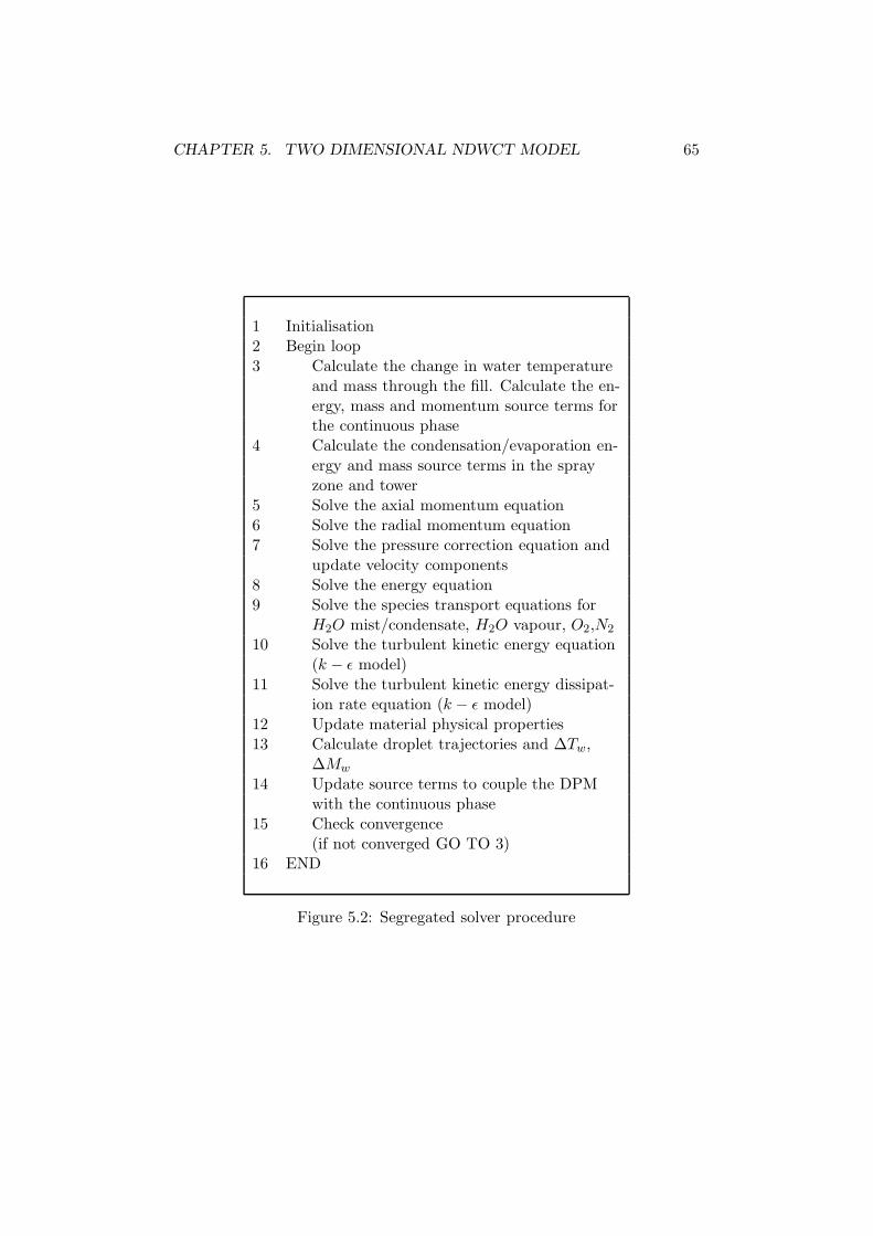
The above procedure together with the equations and numerical proce-
dures outlined in Chapter 3 are solved in FLUENT. The solution procedure
for the segregated solver with the subroutines for the fill and the discrete
phase model (DPM) is depicted in Fig. 5.2. The source terms in the fill
are updated every iteration. The DPM and the source terms coupling the
heat, mass and momentum transfer with the continuous phase are updated
every ten iterations. The solution proceeds until convergence. The solution
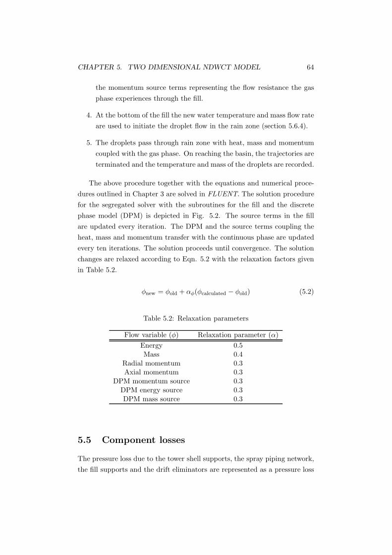
changes are relaxed according to Eqn. 5.2 with the relaxation factors given
in Table 5.2.
φnew = φold + αφ(φcalculated − φold) (5.2)
Table 5.2: Relaxation parameters
Flow variable (φ) Relaxation parameter (α)
Energy 0.5Mass 0.4
Radial momentum 0.3Axial momentum 0.3
DPM momentum source 0.3DPM energy source 0.3DPM mass source 0.3
5.5 Component losses
The pressure loss due to the tower shell supports, the spray piping network,
the fill supports and the drift eliminators are represented as a pressure loss
CHAPTER 5. TWO DIMENSIONAL NDWCT MODEL 65
1 Initialisation2 Begin loop3 Calculate the change in water temperature
and mass through the fill. Calculate the en-ergy, mass and momentum source terms forthe continuous phase
4 Calculate the condensation/evaporation en-ergy and mass source terms in the sprayzone and tower
5 Solve the axial momentum equation6 Solve the radial momentum equation7 Solve the pressure correction equation and
update velocity components8 Solve the energy equation9 Solve the species transport equations for
H2O mist/condensate, H2O vapour, O2,N2
10 Solve the turbulent kinetic energy equation(k − ǫ model)
11 Solve the turbulent kinetic energy dissipat-ion rate equation (k − ǫ model)
12 Update material physical properties13 Calculate droplet trajectories and ∆Tw,
∆Mw
14 Update source terms to couple the DPMwith the continuous phase
15 Check convergence(if not converged GO TO 3)
16 END
Figure 5.2: Segregated solver procedure
CHAPTER 5. TWO DIMENSIONAL NDWCT MODEL 66
@@@R
@@
@@R
Spray nozzles (Kwdn)
Drift eliminators and fill supports (Kde + Kfs)
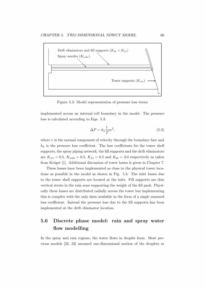
Tower supports (Kcts) -
Figure 5.3: Model representation of pressure loss terms
implemented across an internal cell boundary in the model. The pressure
loss is calculated according to Eqn. 5.3:
∆P = kL1
2ρv2, (5.3)
where v is the normal component of velocity through the boundary face and
kL is the pressure loss coefficient. The loss coefficients for the tower shell
supports, the spray piping network, the fill supports and the drift eliminators
are Kcts = 0.5, Kwdn = 0.5, Kfs = 0.5 and Kde = 3.0 respectively as taken
from Kroger [1]. Additional discussion of tower losses is given in Chapter 7.
These losses have been implemented as close to the physical tower loca-
tions as possible in the model as shown in Fig. 5.3. The inlet losses due
to the tower shell supports are located at the inlet. Fill supports are thin
vertical struts in the rain zone supporting the weight of the fill pack. Physi-
cally these losses are distributed radially across the tower but implementing
this is complex with the only data available in the form of a single summed
loss coefficient. Instead the pressure loss due to the fill supports has been
implemented at the drift eliminator location.
5.6 Discrete phase model: rain and spray water
flow modelling
In the spray and rain regions, the water flows in droplet form. Most pre-
vious models [22, 23] assumed one-dimensional motion of the droplets or
CHAPTER 5. TWO DIMENSIONAL NDWCT MODEL 67
Droplet
Continuous Phase Cell
Droplet
Trajectory
Momentum, Heat
and Mass Transfer
@@
@R
Figure 5.4: Coupling of droplet flow with continuous phase model
represented them more coarsely through average transfer coefficients [5, 24].
Here the droplet flow has been modelled using Lagrangian particle tracking
with coupled heat and mass transfer between the droplets and the continu-
ous phase. The process is shown in Fig. 5.4. The material properties and
equation of state relations for this phase are given in Appendix B.
5.6.1 Droplet trajectory calculation
The droplet trajectory is calculated in the Lagrangian reference frame. The
droplet location is advanced in the x-direction by the step wise integration
of:dx
dt= ud. (5.4)
The instantaneous velocity in the x direction ud is found from a force
balance upon the droplet, equating the droplet inertia with drag and the
body force of gravity. Again for the x-direction this can be written as:
dud
dt= FD(u − ud) +
gx(ρd − ρ∞)
ρd, (5.5)
where FD(u − ud) is the drag force per unit mass and,
FD =18µ
ρdd2d
CDRed
24, (5.6)
CHAPTER 5. TWO DIMENSIONAL NDWCT MODEL 68
and the drag coefficient, CD, is calculated using Eqn. 5.7,
CD = a1 +a2
Red+
a3
Red2 , (5.7)
where the coefficients a1, a2, a3 are taken from Morsi and Alexander [100].
The droplet Reynolds number, Red, is given by,
Red ≡ ρdd |ud − u∞|µ
. (5.8)
The droplet trajectory is determined advancing the droplet location over
small discrete time intervals with the step-wise integration in each coordinate
direction of Eqn. 5.4 in time and Eqn. 5.5 in space. These equations are
discretised using a trapezoidal scheme. The new particle velocity at time
n + 1 is found using:
un+1d =
und (1 − 1
2∆tFD) + ∆tFD
(un∞
+ 12∆tun
d · ∇un∞
)+ ∆t gx(ρd−ρ∞)
ρd
1 + 12∆tFD
.
(5.9)
The new droplet location, xn+1d , can then be found using:
xn+1d = xn
d +1
2∆t(un
d + un+1d
). (5.10)
The time step for the integration ∆t has been set by specifying λ, the
number of time steps to be computed as a droplet crosses a cell. FLUENT
estimates ∆t∗, the droplet residence time in a cell and the time step for
integration is computed using:
∆t =∆t∗
λ. (5.11)
In this study λ has been set to 5.
5.6.2 Heat and mass transfer
This section closely follows the combined heat and mass transfer discussion
in Chapter 2. In FLUENT, the temperature change of the evaporating water
droplet is described in the Lagrangian reference frame as given in Eqn. 5.12:
mdCddTd
dt= hAd(T∞ − Td) +
dmd
dtifgwo. (5.12)
CHAPTER 5. TWO DIMENSIONAL NDWCT MODEL 69
The term hAd(T∞ − Td) represents the sensible heat transfer between the
gas phase and the droplet and dmd
dt ifgwo the latent heat transfer from evap-
oration. ifgwo is the latent heat of water at 0oC. T∞ is the temperature in
Kelvin of the gas phase in the cell that the droplet is currently in, Td is the
droplet temperature, Ad is the droplet surface area, h is the heat transfer
coefficient, ifgwo is the latent heat of vaporisation, Cp is the specific heat of
water evaluated at the droplet temperature and md is the droplet mass in
kg.
The mass transfer from the droplet due to evaporation is described by:
N = kc(Cs − C∞), (5.13)
where N is the molar flux of vapour species with units (kgmol/m2s), kc is the
mass transfer coefficient m/s and C∞ is the concentration of water vapour
in the bulk gas phase (kgmol/m3). Cs is the molar concentration of water
vapour at the droplet surface, calculated assuming the vapour pressure at
the droplet surface is equal to the saturated vapour pressure Psat, calculated
at the droplet temperature. Cs and C∞ are given by Eqn. 5.14 and Eqn.
5.15 respectively:
Cs =Psat,Td
RTd, (5.14)
C∞ = XPop
RT∞
, (5.15)
where R is the universal gas constant, Pop is the operating pressure and X
is the mole mass fraction of the evaporating species. The new droplet mass
is updated following Eqn. 5.16:
md(t + ∆t) = md(t) − NAdMw∆t, (5.16)
where Mw is the molecular weight of water in kg/kmol. The heat and mass
transfer coefficients used in these equations are derived from the empirical
correlations given in Eqn. 5.17 and Eqn. 5.18 below. These correlations,
taken from [1, 40], are valid for 2 ≤ Red ≤ 800. In this study the droplet
Reynolds number in the spray zone is Red ≈ 1000 − 1200, just above the
upper limit of the correlation. In the rain zone 15 . Red . 1400. While the
upper range in the rain zone is somewhat above the limits of the empirical
correlation, the mean Red based on the average conditions in the rain zone
CHAPTER 5. TWO DIMENSIONAL NDWCT MODEL 70
and sauter mean diameter of the droplet distribution, is Red ≈ 430 which is
in the middle of the valid range for the correlations, so is reasonable for use
in this study.
Sh =hDdd
Dm= 2.0 + 0.6Re
1/2d Sc1/3 (5.17)
Nu =hdd
k∞= 2.0 + 0.6Re
1/2d Pr1/3 (5.18)
If the droplet temperature falls below the dew point temperature of the
gas phase then condensation would naturally occur. However under these
conditions, the droplet is treated as inert in FLUENT and no mass transfer
occurs. Condensation of water vapour and evaporation of mist/condensate
in the gas phase are discussed in the next section.
5.6.3 Discrete phase-continuous phase coupling
The heat, mass and momentum transfer from the discrete phase is coupled
with the continuous phase through source terms as given below and depicted
in Fig. 5.4. The momentum source (Smom) or sink in the continuous phase
due to the change in droplet momentum across a cell control volume is given
in Eqn. 5.19.
Smom =
(18µCDRed
ρdd2d24
(ud − u∞)
)md∆t (5.19)
The evaporation from the droplets is coupled with the continuous phase
through the vapour transport equation and the continuity equation. The
source term is given by Eqn. 5.20,
Sv = ∆md, (5.20)
where ∆md is the change in droplet mass across a cell control volume. Sim-
ilarly the energy source term for the gas phase is given by Eqn. 5.21,
Sq = mdCp∆Td + ∆md
(− ifgwo +
Td∫
Tref
CpdT), (5.21)
where ∆Tp and ∆mp are the changes in temperature and mass of the droplet
across a cell and Tref is 273.15 Kelvin.
In this model, there is the potential for the gas phase to become super-
saturated. In cells where this occurs a separate algorithm is run iteratively
CHAPTER 5. TWO DIMENSIONAL NDWCT MODEL 71
if (RH >1 ) or (if RH <1 and φmist >0) then:Sv = Sv + C(ω′′ − ω)Smist = −Sv
Sq = ifgwoSmist
Figure 5.5: Condensation routine procedure
to ensure that any additional vapour in the gas phase in excess of the sat-
uration level is transfered to the condensate component of the continuous
phase with the latent heat source put back into the vapour mixture. Simi-
larly if the gas phase becomes unsaturated then the condensate evaporates
with the latent heat absorbed from the continuous phase. The procedure is
outlined in Fig. 5.5, where C = 0.6, Sv is the vapour source, Smist is the
condensate/mist source and Sq is the energy source term.
5.6.4 Spray and rain zone modelling
Spray zone
Large cooling towers use spray nozzles that operate at relatively low pres-
where the smoothing factor f =(0.9−Lfi)(0.9−0.6) for 0.6 < Lfi < 0.9. This approach
was found to give smoother fit to the data in the range of air and water flow
rates considered here than a single general correlation developed for all fill
depths and water flow rates using Eqn. 5.28.
The implementation of this routine has been tested against the experi-
mental data in Kloppers thesis [3] found to return the correct pressure drop.
5.7.3 Heat and mass transfer in the fill
The heat and mass transfer characteristics of the fill are derived from em-
pirical transfer coefficients in the form of the Poppe Merkel number. The
correlations for the fill type in the reference tower were not available so other
data given in Kloppers’ thesis [3] for a similar film fill, have been used.
As the heat and mass transfer characteristics of the fill are defined
through the Merkel number for the Poppe method, any method implemented
in this numerical model must be equivalent to the Poppe method. Because
the Poppe method does not introduce any additional assumptions into the
model, other than the one dimensional ones discussed in section 2.2 and sec-
tion 5.7.1, this becomes very easy. The heat and mass transfer is specified
through Eqns. 2.1-2.4.
The empirical transfer coefficients conveniently yield the heat and mass
transfer coefficients together with the contact area between the phases. With
hmA known, the product of the heat transfer coefficient and contact surface
area, hA, can be found by re-arranging the Lewis factor relationship,
Lef =h
hmCpm, (5.34)
to give,
hA = LefhmACpm. (5.35)
Following Poppe’s approach [10], the Lewis factor can be found from Bosj-
CHAPTER 5. TWO DIMENSIONAL NDWCT MODEL 78
nakovics formula [1],
Lef = 0.8652/3 ·
(ω′′
Tw+0.622ω+0.622 − 1
)
ln
(ω′′
Tw+0.622
ω+0.622
) . (5.36)
Bosjnakovics formula under saturation conditions is modified, as shown in
Appendix A. The transfer coefficient used here is written in terms of the fill
air and water inlet flow rates, as shown in Eqns. 5.37-5.39 (taken from [3]):
MeP,0.6m
Lfi=
hmA
mwLfi
= 1.497125G0.276216w G0.665735
a
− 0.589942G0.634757w G0.622408
a (5.37)
MeP,0.9m
Lfi=
hmA
mwLfi
= 1.526182G0.078237w G0.695680
a
− 0.556982G0.419584w G0.675151
a (5.38)
MeP,1.2m
Lfi=
hmA
mwLfi
= 1.380517G0.112753w G0.698206
a
− 0.517075G0.461071w G0.681271
a (5.39)
The above relations give the Poppe Merkel number per unit fill depth and
as for the loss coefficients, the correlations are developed at discrete fill
depths of 0.6m, 0.9m and 1.2m, with experimental data over the range
2.7kg/s/m2 < Gw < 6.1kg/s/m2 and 1.2kg/s/m2 < Ga < 4.2kg/s/m2 [3,
61]. Again, operating point for the reference cooling tower modelled in this
study is at a mass flux of Gw = 2.21kg/s/m2 slightly below this range of
experimental data. The difference is small however and has been deemed
acceptable in this work.
CHAPTER 5. TWO DIMENSIONAL NDWCT MODEL 79
The data in Kloppers’ thesis [3] has also been used here to develop a
general correlation for the Poppe Merkel number as a function of fill depth,
MeP,gen
Lfi=
hmA
mwLfi= 1.118G−0.389
w G0.735a L−0.280
fi . (5.40)
The regression analysis used was similar to that used by Kloppers [3] to fit
the same data to a general correlation using the Merkel model (Eqn. 7.5).
The regression analysis used here successfully reproduced Kloppers other
correlations. The correlation R2 value for this fitted equation is 0.9873.
This equation has been used for the cases where the fill depth simulated did
not match one of the three given above.
5.7.4 Coupling procedure
The calculations across each layer take place between the averaged continu-
ous phase flow variables and the water flow variables on the one dimensional
grid (Fig. 5.7). The source terms calculated are identical for all the cells
across the layer.
The water evaporated, mmevap, across fluid layer m is determined using
Eqn. 5.41, where ω is the average specific humidity in the fluid zone and
∆Lfi is the height of the current layer. If the air is super-saturated then
Eqn. 5.42 is used:
mmevap = hmA
(∆Lfi
Lfi
)(ωm
sat,Tw − ωm), (5.41)
mmevap = hmA
(∆Lfi
Lfi
)(ωm
sat,Tw − ωmsat,Ta). (5.42)
The equivalent relation for Eqn. 5.41 in Chapter 2 is Eqn. 2.1. Eqn. 5.42 is
equivalent to Eqn. A.30 in Appendix A. The downstream water mass flow
rate is found using Eqn. 5.43:
mnw = mn+1
w − mmevap. (5.43)
The latent and sensible heat transfer is evaluated using Eqns. 5.44 and 5.45
CHAPTER 5. TWO DIMENSIONAL NDWCT MODEL 80
respectively (c.f. Eqn. 2.4 and 2.5 in Chapter 2):
qmlatent = mm
evapifgwo, (5.44)
qmsensible = hA((T n+1
w + T nw)/2 − Tm
a ), (5.45)
where Tma is the average temperature of the continuous phase in the layer.
The water temperature at the inter-facial layer n is determined using:
T nw = T n+1
w − (qmsensible + qm
latent)
Cpwmn+1w
. (5.46)
When the flow becomes super-saturated, water vapour condenses as mist
(mmcond) and the latent heat of vaporisation is released into the mixture. It
has been assumed for this investigation, as in the Poppe model [3, 10],
that vapour condenses as mist when the vapour pressure rises above the
saturation vapour pressure.
The mass source Ms and enthalpy source Qs per unit volume are given
by Eqns. 5.47 and 5.48:
Mms =
mmevap
∆Lfi, (5.47)
Qms = (mn+1
w Cpw∆Tmw + mm
evap(Cpv(Tn+1w + T n
w)/2
−298.15) − ifgwo))/∆Lfi + mmcondifgwo. (5.48)
5.7.5 Model validation
In order to validate this approach, it has been compared against the pre-
dictions of the Poppe model described in Chapter 2. The Poppe equations
(see Appendix A) were numerically integrated using the non-stiff ODE45
Runge-Kutta numerical integration procedure in Matlab [103], a commer-
cial mathematical programing software. The ODE45 procedure uses an au-
tomatic step size selection algorithm which in this case reaches completion
after approximately 70 discrete steps. The comparison has been performed
under the conditions given in Table 5.4. The air and water fluid properties
are based on those in Kroger [1] and are given in Appendix 1.
The Poppe model solution and the CFD routine with 40 nodes/layers
through the fill are compared with and without the effects of condensation
included. For both methods, ignoring condensation here simply means ig-
CHAPTER 5. TWO DIMENSIONAL NDWCT MODEL 81
Table 5.4: Test parameters
ωi 0.012kg/kgTw,i 40oCTa,i 20oCGa 1.5kg/s/m2
Gw,i 2.4kg/s/m2
MEp 1.0δME 5 × 10⁻⁵
δω 1 × 10⁻⁴
noring the switch to use the alternate equations when the relative humidity
rises above 100%. This has been done to demonstrate the importance of
condensation to the problem.
The comparison of the two models is given in Figs. 5.8-5.9 at an air
mass flux of Ga = 1.5kg/s/m2 and Ga = 2.5kg/s/m2 respectively. The
water temperature, air temperature and relative humidity have been plot-
ted against Poppe Merkel number as the numerical integration proceeds,
showing how the solutions diverge when saturation in not included.
The importance of condensation in the calculation is clear. When con-
densation is ignored, the relative humidity is allowed to rise above 100% and
the two solutions diverge. If latent heat is released, the energy and mass bal-
ance changes significantly, with the air temperature rising when saturation
is included. The water outlet temperature does not register a noticeable
change however. In a full NDWCT calculation, the inaccurate prediction
of the air temperature leaving the fill could lead to an under-estimate the
tower draft and therefore the air-flow rate. This could then lead to a more
significant change in water outlet temperature. The curves for the Poppe
model and the CFD model match well, both with and without condensa-
tion indicating that the physics of the problem is well captured in the CFD
model and that the models are essentially equivalent.
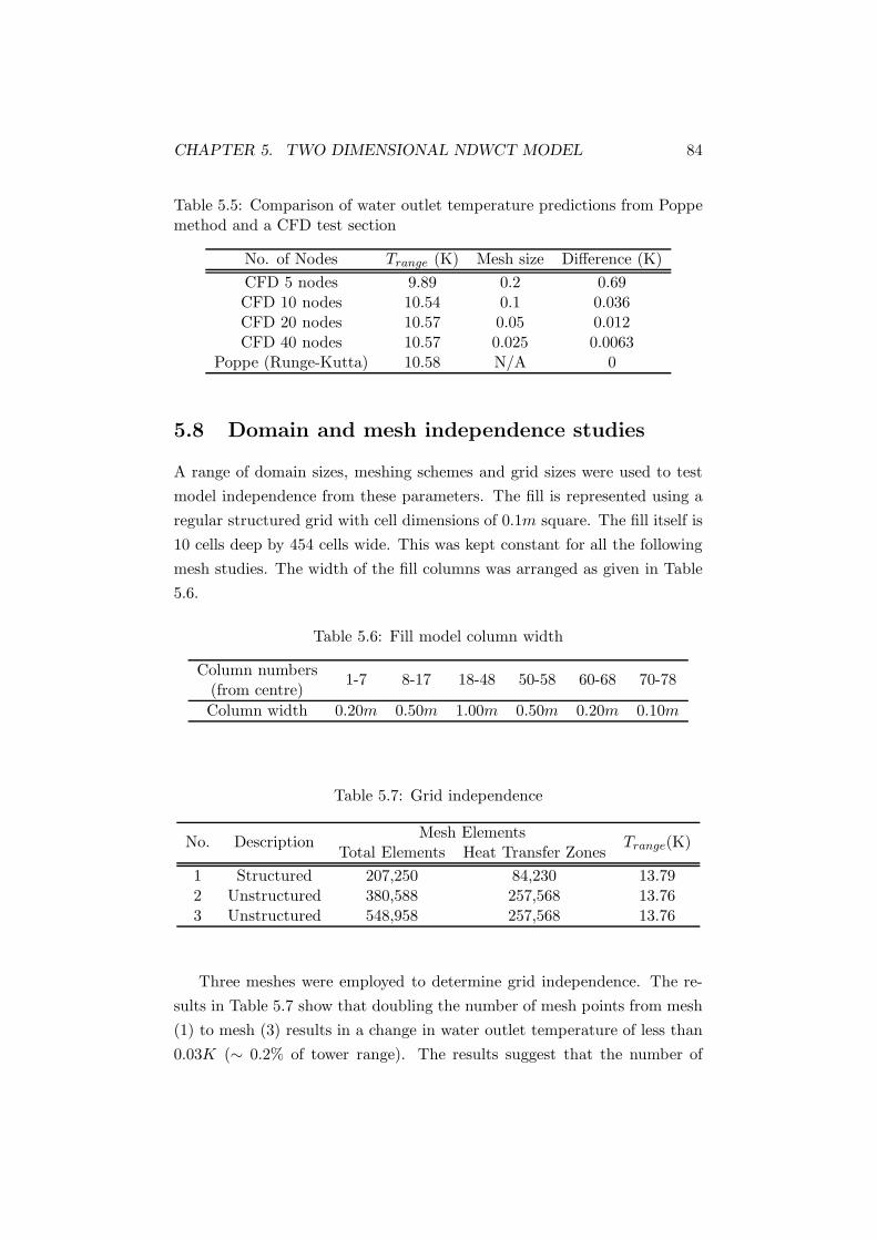
Table 5.5 gives a comparison of the predicted water outlet temperature
from the Poppe method and the CFD numerical procedure under the con-
ditions in Table 5.4. With greater than five nodes through the depth, there
is very little improvement in model prediction. In this work ten nodes or
layers were used.
CHAPTER 5. TWO DIMENSIONAL NDWCT MODEL 82
0 0.1 0.2 0.3 0.4 0.5 0.6 0.7 0.8 0.9 120
22
24
26
28
30
32
34
Air
Tem
pera
ture
(o C)
Poppe Merkel No.
CFD (sat)CFD (unsat)Poppe (sat)Poppe (unsat)
(a)
0 0.1 0.2 0.3 0.4 0.5 0.6 0.7 0.8 0.9 128
30
32
34
36
38
40
Wat
er T
empe
ratu
re (o C
)
Poppe Merkel No.
CFD (sat)CFD (unsat)Poppe (sat)Poppe (unsat)
(b)
0 0.1 0.2 0.3 0.4 0.5 0.6 0.7 0.8 0.9 10.8
0.85
0.9
0.95
1
1.05
1.1
1.15
Rel
ativ
e H
umid
ity
Poppe Merkel No.
CFD (sat)CFD (unsat)Poppe (sat)Poppe (unsat)
(c)
Figure 5.8: Comparison of heat and mass transfer characteristics of Poppemethod and equivalent CFD implementation through the depth of the fillwith Ga = 1.5kg/s/m2
CHAPTER 5. TWO DIMENSIONAL NDWCT MODEL 83
0 0.1 0.2 0.3 0.4 0.5 0.6 0.7 0.8 0.9 120
21
22
23
24
25
26
27
28
29
30
Air
Tem
pera
ture
(o C)
Poppe Merkel No.
CFD (sat)CFD (unsat)Poppe (sat)Poppe (unsat)
(a)
0 0.1 0.2 0.3 0.4 0.5 0.6 0.7 0.8 0.9 128
30
32
34
36
38
40
Wat
er T
empe
ratu
re (o C
)
Poppe Merkel No.
CFD (sat)CFD (unsat)Poppe (sat)Poppe (unsat)
(b)
0 0.1 0.2 0.3 0.4 0.5 0.6 0.7 0.8 0.9 10.8
0.85
0.9
0.95
1
1.05
1.1
1.15
Rel
ativ
e H
umid
ity
Poppe Merkel No.
CFD (sat)CFD (unsat)Poppe (sat)Poppe (unsat)
(c)
Figure 5.9: Comparison of heat and mass transfer characteristics of Poppemethod and equivalent CFD implementation through the depth of the fillwith Ga = 2.5kg/s/m2
CHAPTER 5. TWO DIMENSIONAL NDWCT MODEL 84
Table 5.5: Comparison of water outlet temperature predictions from Poppemethod and a CFD test section
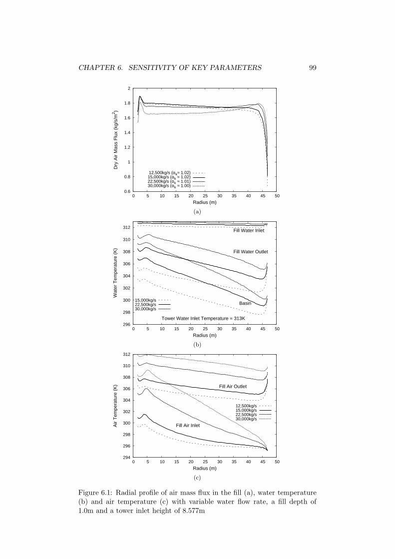
Figure 6.1: Radial profile of air mass flux in the fill (a), water temperature(b) and air temperature (c) with variable water flow rate, a fill depth of1.0m and a tower inlet height of 8.577m
CHAPTER 6. SENSITIVITY OF KEY PARAMETERS 100
0
20
40
60
80
100
0 5 10 15 20 25 30 35 40 45 50
% W
ater
Tem
pera
ture
Dro
p pe
r Z
one
Radius (m)
Rain Zone (%)
Fill Zone (%)
Spray Zone (%)
12,500kg/s15,000kg/s22,500kg/s30,000kg/s
(a)
0
20
40
60
80
100
120
140
160
180
200
0 5 10 15 20 25 30 35 40 45 50
Ga
(i ma,
o -
i ma,
i) (k
W/m
2 )
Radius (m)
Fill Air Outlet
Fill Air Inlet12500kg/s15000kg/s22500kg/s30000kg/s
(b)
10
20
30
40
50
60
70
0 5 10 15 20 25 30 35 40 45 50
Cp w
(T
w,i-
Tw
,o)
(kW
/kg
wat
er)
Radius (m)
12,500kg/s15,000kg/s22,500kg/s30,000kg/s
(c)
Figure 6.2: Radial profile of local water temperature drop per zone (a),cumulative heat transfer to air (b) and local cooling load (c) with variablewater flow rate, a fill depth of 1.0m and a tower inlet height of 8.577m
CHAPTER 6. SENSITIVITY OF KEY PARAMETERS 101
0.005
0.01
0.015
0.02
0.025
0.03
0.035
0.04
0.045
0.05
0 5 10 15 20 25 30 35 40 45 50
ω
Radius (m)
Fill Air Inlet
Fill Air Outlet
12500kg/s15000kg/s22500kg/s30000kg/s
Figure 6.3: Radial profile of specific humidity at the fill inlet with variablewater flow rate, a fill depth of 1.0m and a tower inlet height of 8.577m
of the cooling range and the spray region less than 10%. The rain zone
accounts for just over 20% of the local cooling range through most of the
tower but at the tower inlet, it rises to almost 40%, where the high speed
airflow at the inlet improves the heat transfer in the rain region, somewhat
counteracting the poorer performance of the fill in this region. The radial
profile of the local cooling load per kg water flow (Cpw(Tw,i−Tw,o)) is given
in Fig. 6.2 (c). The largely uniform axial air flow through the fill suggests
that the non-uniform water outlet temperature and local cooling load profile
is largely a function of the air temperature and humidity as it enters the
fill. The air temperature at the centre of the tower is almost 6K warmer
than the ambient air at the inlet (Fig. 6.1 (c)). The humidity also increases
significantly through the rain zone (Fig. 6.3), reducing the driving force for
heat transfer at the centre of the tower. This non-uniformity of heat transfer
can be seen clearly in Fig. 6.2 (b), where the total heat transfered to the
air from the tower inlet to the fill inlet and then to the fill outlet is plotted
per unit fill area (Ga(ima,o − ima,i)).
The profiles of the specific humidity across the tower, both at the inlet
to the fill and at the top of the fill can be seen in Fig. 6.3. The interesting
phenomena noted in section 5.11, where the humidity increases faster than
the air temperature due to the non-uniform droplet distribution, can be
seen in this figure. In Fig. 6.1 (c) the air temperature increases very slowly
CHAPTER 6. SENSITIVITY OF KEY PARAMETERS 102
through the outer rain region whereas the specific humidity profile in Fig.
6.3 shows that the evaporation increases almost linearly throughout the rain
zone. This is further discussed in secion 6.2.6.
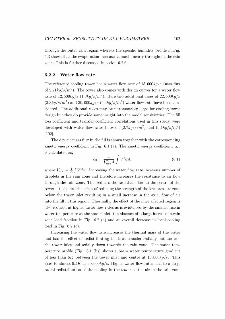
6.2.2 Water flow rate
The reference cooling tower has a water flow rate of 15, 000kg/s (mas flux
of 2.21kg/s/m2). The tower also comes with design curves for a water flow
rate of 12, 500kg/s (1.8kg/s/m2). Here two additional cases of 22, 500kg/s
(3.3kg/s/m2) and 30, 000kg/s (4.4kg/s/m2) water flow rate have been con-
sidered. The additional cases may be unreasonably large for cooling tower
design but they do provide some insight into the model sensitivities. The fill
loss coefficient and transfer coefficient correlations used in this study, were
developed with water flow rates between (2.7kg/s/m2) and (6.1kg/s/m2)
[102].
The dry air mass flux in the fill is shown together with the corresponding
kinetic energy coefficient in Fig. 6.1 (a). The kinetic energy coefficient, αk,
is calculated as,
αk =1
V 3aveA
∫V 3dA, (6.1)
where Vave = 1A
∫V dA. Increasing the water flow rate increases number of
droplets in the rain zone and therefore increases the resistance to air flow
through the rain zone. This reduces the radial air flow to the centre of the
tower. It also has the effect of reducing the strength of the low pressure zone
below the tower inlet resulting in a small increase in the axial flow of air
into the fill in this region. Thermally, the effect of the inlet affected region is
also reduced at higher water flow rates as is evidenced by the smaller rise in
water temperature at the tower inlet, the absence of a large increase in rain
zone load fraction in Fig. 6.2 (a) and an overall decrease in local cooling
load in Fig. 6.2 (c).
Increasing the water flow rate increases the thermal mass of the water
and has the effect of redistributing the heat transfer radially out towards
the tower inlet and axially down towards the rain zone. The water tem-
perature profile (Fig. 6.1 (b)) shows a basin water temperature gradient
of less than 6K between the tower inlet and centre at 15, 000kg/s. This
rises to almost 9.5K at 30, 000kg/s. Higher water flow rates lead to a large
radial redistribution of the cooling in the tower as the air in the rain zone
CHAPTER 6. SENSITIVITY OF KEY PARAMETERS 103
is heated severely towards the tower centre (Fig. 6.1 (c)) and the air flow is
also slightly reduced in this region. The radial re-distribution of cooling in
the tower is also well shown in Fig. 6.2 (c), with a more pronounced cooling
load gradient from tower centre to tower inlet. The axial re-distribution of
the cooling load from the fill to the rain zone at higher water flow rates can
best be seen in Fig. 6.2 (a). At a flow rate of 15, 000kg/s, the rain zone
contributes around 20% of the local cooling range whereas at 30, 000kg/s,
it rises to almost 40%. At higher water flow rates, the heat and mass trans-
fer is greater in the rain zone. Hence the air entering the fill is at higher
temperature and humidity which results in a proportional reduction in heat
and mass transfer in this region.
6.2.3 Fill depth
Three fill depths have been tested, 0.6m, 0.9m and 1.2m. Varying the fill
height over this range does not introduce any significant change to the non-
uniformity of the air flow (Fig. 6.4 (a)), the water outlet temperature (Fig.
6.4 (b)) or the cooling load distribution (Fig. 6.5 (a-c)). The deeper fill
has a more uniform air-flow profile due to the increased flow restriction in
the tower. At low fill depths the air flow increases slightly to the centre,
increasing the kinetic energy coefficient from 1.01 at a fill depth of 1.2m to
1.03 at a fill depth of 0.6m.
The axial distribution of cooling load between the spray, fill and rain
zones is also fairly constant, although at 0.6m fill depth the rain zone starts
to occupy a higher percentage of the total cooling. This is because the water
entering the rain zone is at a higher temperature so the heat transfer here
improves and this region becomes relatively more effective (Fig. 6.5 (a)).
This gives some insight into the effect of an optimal fill depth selection.
There is very little increase in cooling load seen between a fill depth of 0.9m
and 1.2m. At a depth of 0.6m however, the fill is insufficiently sized such
that a small increase in fill depth returns a large increase in water cooling.
6.2.4 Tower inlet height
Here three inlet heights are examined, 8.577m, 6.777m and 4.977m. The
reference design height is 8.577m. Reducing the tower inlet height reduces
the flow area into the tower, increasing the flow restriction and increasing
Figure 6.4: Radial profile of air mass flux in the fill (a), water temperature(b) and air temperature (c) with variable fill depth, a water flow rate of15000kg/s and a tower inlet height of 8.577m
CHAPTER 6. SENSITIVITY OF KEY PARAMETERS 105
0
20
40
60
80
100
0 5 10 15 20 25 30 35 40 45 50
% W
ater
Tem
pera
ture
Dro
p pe
r Z
one
Radius (m)
Rain Zone (%)
Fill Zone (%)
Spray Zone (%)
depth = 0.6mdepth = 0.9mdepth = 1.2m
(a)
0
20
40
60
80
100
120
140
160
0 5 10 15 20 25 30 35 40 45 50
Ga
(i ma,
o -
i ma,
i) (k
W/m
2 )
Radius (m)
Fill Air Outlet
Fill Air Inlet
fill depth = 0.6mfill depth = 0.9mfill depth = 1.2m
(b)
30
35
40
45
50
55
60
65
70
0 5 10 15 20 25 30 35 40 45 50
Cp w
(T
w,i-
Tw
,o)
(kW
/kg
wat
er)
Radius (m)
depth = 0.6mdepth = 0.9mdepth = 1.2m
(c)
Figure 6.5: Radial profile of local water temperature drop per zone (a),cumulative heat transfer to air (b) and local cooling load (c) with variablefill depth, a water flow rate of 15000kg/s and a tower inlet height of 8.577m
CHAPTER 6. SENSITIVITY OF KEY PARAMETERS 106
0.005
0.01
0.015
0.02
0.025
0.03
0.035
0.04
0 5 10 15 20 25 30 35 40 45 50
ω
Radius (m)
Fill Air Outlet
Fill Air Inlet
fill depth 0.6mfill depth 0.9mfill depth 1.2m
Figure 6.6: Radial profile of specific humidity with variable fill depth, awater flow rate of 15000kg/s and a tower inlet height of 8.577m
the air velocity beneath the fill. The radial velocity of the air entering the
tower at the inlet is given in Fig. 6.7. The maximum velocity of the flow
at an inlet height of 4.977m is ∼ 50% larger than that at an inlet height of
8.577m. This has the effect of further decreasing the pressure below the fill
at the inlet which further retards the axial flow into the fill in this region
(Fig. 6.8 (a)). The kinetic energy coefficient rises from 1.02 at an inlet
height of 8.577m to 1.05 at an inlet height of 4.977m. The size of the inlet
effected region remains almost the same at approximately 3.5m of the radius
under all cases tested (Fig. 6.8 (b)). Although the performance degradation
in this region does increase a little with reduced inlet height, the overall
effect of the region remains negligible. If the effect of the inlet was removed
and the temperature maintained at the minimum basin temperature, the
overall water outlet temperature would be reduced by only 0.14K for the
4.977m case and by 0.06K for the 8.577m case.
Surprisingly, the load fraction in the rain zone does not change much with
inlet height, with the heat transfer reduced in equal proportion through all
the heat transfer zones. Initial expectations were that the reduced droplet
residence time in the rain zone, due to the lower rain zone, would lead to
severely reduced rain zone performance. The combination of the higher
air velocity through the rain zone and the poorer performance on the other
regions in the tower (due to lower overall air flow rate), means the proportion
CHAPTER 6. SENSITIVITY OF KEY PARAMETERS 107
0 0.25 0.5 0.75 1U/U
max
0
0.2
0.4
0.6
0.8
1
y/h
height = 4.977mheight = 6.777mheight = 8.577m
Figure 6.7: Radial velocity magnitude at the tower inlet with r = 46.5m,where Umax = 6.5(m/s) for h = 4.977m, Umax = 5.55(m/s) for h = 6.777mand Umax = 5.0(m/s) for h = 8.577m
Figure 6.8: Radial profile of air mass flux in the fill (a), water temperature(b) and air temperature (c) with variable tower inlet height, a water flowrate of 15000kg/s and a fill depth of 1.0m
Figure 6.9: Radial profile of local water temperature drop per zone (a),cumulative heat transfer to air (b) and local cooling load (c) with variabletower inlet height, a water flow rate of 15000kg/s and a fill depth of 1.0m
Figure 6.11: Total mass transfer from droplets to the gas phase along avertical slice through the rain zone, at a radius of (a) 20m, (b) 30m and (c)40m
Figure 6.12: Total sensible heat transfer between the rain zone droplets andthe gas phase along a vertical slice through the rain zone, at a radius of (a)20m, (b) 30m and (c) 40m
CHAPTER 6. SENSITIVITY OF KEY PARAMETERS 113
greatest. With the lower inlet height, the mass transfer is slightly higher
due to the increased air velocity.
The plots illustrate how different the behaviour is with the uniform and
non-uniform droplet distributions. The sensible heat transfer with the non-
uniform distribution goes slightly negative, which means the air is on average
heating the water. This only occurs in the outer regions of the tower with
inlet height of 8.577m. It is important to note that this sensible heat transfer
is a total value, meaning that on average the smaller droplets are heated
more than the larger droplets are cooled. Individual droplets may be heated
in other regions as well, but the total sensible heat transfer between the air
and all the droplets in those regions is positive.
The plots show that latent heat transfer is the dominant mechanism for
reducing water temperature. With an evaporation rate of ∼ 0.0015kg/s/m3 ,
the heat transfer due to evaporation is about 3.6kW/m3. Through most of
the tower, the sensible heat transfer experienced by the gas phase is close
to zero or negative (with the non-uniform droplet distribution).
6.2.5 Ambient air condition
As the inlet air temperature is raised, the density difference between the
inside of the tower and the ambient surroundings is reduced. The tower
draft is therefore reduced and so is the overall air mass flow rate (Fig. 6.13
(a)). The effect of the reduced air flow rate and increased air temperature
and humidity on water temperature and heat transfer in all zones can be
seen clearly in Fig. 6.13 (b) and Fig. 6.14 (c). The heat transfer is reduced
nearly uniformly across the tower. Humidity has a much smaller effect on
the tower performance, the changes in ambient specific humidity being quite
small relative to the changes in humidity experienced through the tower as
shown in Fig. 6.15.
The air temperature at the inlet to the fill is much more uniform across
the tower at an air temperature of 300K than at 285K. The reduction in the
difference between the water temperature and air temperature, decreases
the sensible heat transfer, such that the air temperature does not rise much
through the rain zone (see Fig. 6.14 (b)). The shape of the energy transfer
profile remains the same however (see Fig. 6.14 (c)), as the mass transfer
rate remains high across the tower and latent heat transfer constitutes over
80% of the total heat transfer in the rain zone. Overall gradient of the
Ta = 285 RH61.4% (αk≈ 1.02) Ta = 300 RH61.4% (αk≈ 1.02)
(a)
290
295
300
305
310
0 5 10 15 20 25 30 35 40 45 50
Wat
er T
empe
ratu
re (
K)
Radius (m)
Fill water inlet
Fill water outlet (Ta=285)
Fill water outlet (Ta=300)
Basin (Ta=285)
Basin (Ta=300)
Ta = 285 RH40%Ta = 300 RH40%
Ta = 285 RH61.4%Ta = 300 RH61.4%
(b)
285
290
295
300
305
310
0 5 10 15 20 25 30 35 40 45 50
Air
Tem
pera
ture
Radius (m)
Fill Air Inlet (Ta=285)
Fill Air Inlet (Ta=300)
Fill Air Outlet (Ta=285)
Fill Air Outlet (Ta=300)
Ta=285 RH40%Ta=300 RH40%
Ta=285 RH61.4%Ta=300 RH61.4%
(c)
Figure 6.13: Radial profile of air mass flux in the fill (a), water temperature(b) and air temperature (c) with variable ambient air temperature and hu-midity, a tower inlet height of 8.577m, a water flow rate of 15,000kg/s anda fill depth of 1.0m
CHAPTER 6. SENSITIVITY OF KEY PARAMETERS 115
0
20
40
60
80
100
0 5 10 15 20 25 30 35 40 45 50
% W
ater
Tem
pera
ture
Dro
p pe
r Z
one
Radius (m)
Rain Zone (%)
Fill Zone (%)
Spray Zone (%)
Ta = 285 RH40%Ta = 300 RH40%
Ta = 285 RH61.4%Ta = 300 RH61.4%
(a)
0
50
100
150
200
250
0 5 10 15 20 25 30 35 40 45 50
Ga
(i ma,
o -
i ma,
i) (k
W/m
2 )
Radius (m)
Fill air outlet
Fill air inlet
Ta=285 RH40%Ta=300 RH40%
Ta=285 RH61.4%Ta=300 RH61.4%
(b)
20
30
40
50
60
70
80
90
0 5 10 15 20 25 30 35 40 45 50
Cp w
(T
w,i-
Tw
,o)
(kW
/kg
wat
er)
Radius (m)
Ta = 285 RH40%Ta = 300 RH40%
Ta = 285 RH61.5%Ta = 300 RH61.5%
(c)
Figure 6.14: Radial profile of local water temperature drop per zone (a),cumulative heat transfer to air (b) and local cooling load (c) with variableambient air temperature and humidity, a tower inlet height of 8.577m, awater flow rate of 15,000kg/s and a fill depth of 1.0m
CHAPTER 6. SENSITIVITY OF KEY PARAMETERS 116
0
0.005
0.01
0.015
0.02
0.025
0.03
0.035
0.04
0 5 10 15 20 25 30 35 40 45 50
ω
Radius (m)
Fill Air Inlet
Fill Air Outlet
Ta = 285 RH40%Ta = 300 RH40%
Ta = 285 RH61.5%Ta = 300 RH61.5%
Figure 6.15: Radial profile of specific humidity with variable ambient airtemperature and humidity, a tower inlet height of 8.577m, a water flow rateof 15,000kg/s and a fill depth of 1.0m
air enthalpy profile remains the same regardless of inlet air temperature or
humidity. The limited effect the inlet conditions have on the mass transfer
profile can be seen in Fig. 6.15. The specific humidity profile remains much
the same across the tower regardless of inlet condition, it is just shifted due
to the change in air flow rate.
Overall, while the effect of ambient air temperature on performance is
significant, the effect of humidity or temperature on non-uniformity of heat
and mass transfer is minimal.
6.2.6 Droplet diameter
The droplet distribution in the rain zone for the reference tower, has a Sauter
mean diameter of 3.26mm (Table 5.3). Here results for the flow with uniform
droplet diameters of 3.26mm, 5.31mm and 7.31mm are also presented.
The droplet diameter is shown to have only a very slight impact on the
radial air-flow rate profile (Fig. 6.16 (a)), both overall and with respect to
any non-uniformity. Again, this is because the restriction through the fill
region dominates the flow.
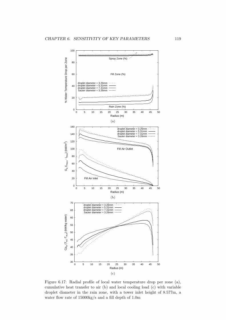
The influence of droplet size on the heat and mass transfer however is
more significant. As the droplet diameter is increased, thereby reducing the
CHAPTER 6. SENSITIVITY OF KEY PARAMETERS 117
total wetted contact area, the heat and mass transfer in the rain zone is
reduced. The air undergoes less heating radially through the rain zone and
the air temperature and humidity at the centre of the tower are decreased
as shown in Fig. 6.16 (c) and Fig. 6.18. This has the effect of increasing the
cooling load in the centre of the tower (Fig. 6.17 (c)). Overall, the cooling
in the rain zone is increased from ∼10% for droplet diameter of 7.31mm and
more than 20% for the case with droplet diameters of 3.26mm.
It is interesting to note the differences in the results for the droplet di-
ameter of 3.26mm and the results for the non-uniform droplet distribution
with a Sauter mean diameter of 3.26mm, shown in Figs. 6.16-6.18. Overall
the tower performance is very similar. With the uniform droplet distribu-
tion, the tower range is 13.80 (K) and with the non-uniform distribution, the
tower range is 13.76 (K). The performance of the rain zone and the overall
non-uniformity of heat and mass transfer is very different however.
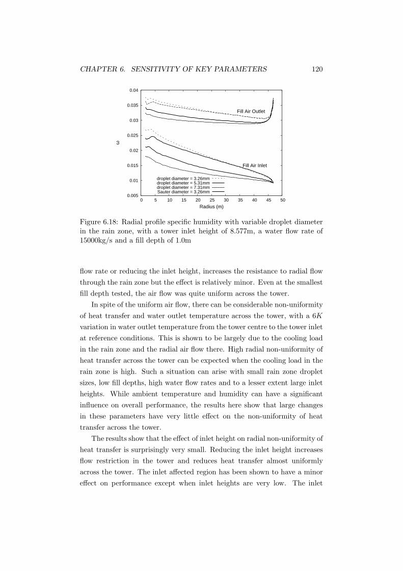
The most interesting feature is that the air temperature profiles are quite
different. The air temperature increases more linearly in the uniform droplet
diameter case (Fig. 6.18) than in the case with the droplet distribution, but
the profiles of specific humidity are quite similar. This is related to the
phenomena noted in section 5.11 and section 6.2.4, where the small water
droplets near the tower inlet are carried further into the tower and cool the
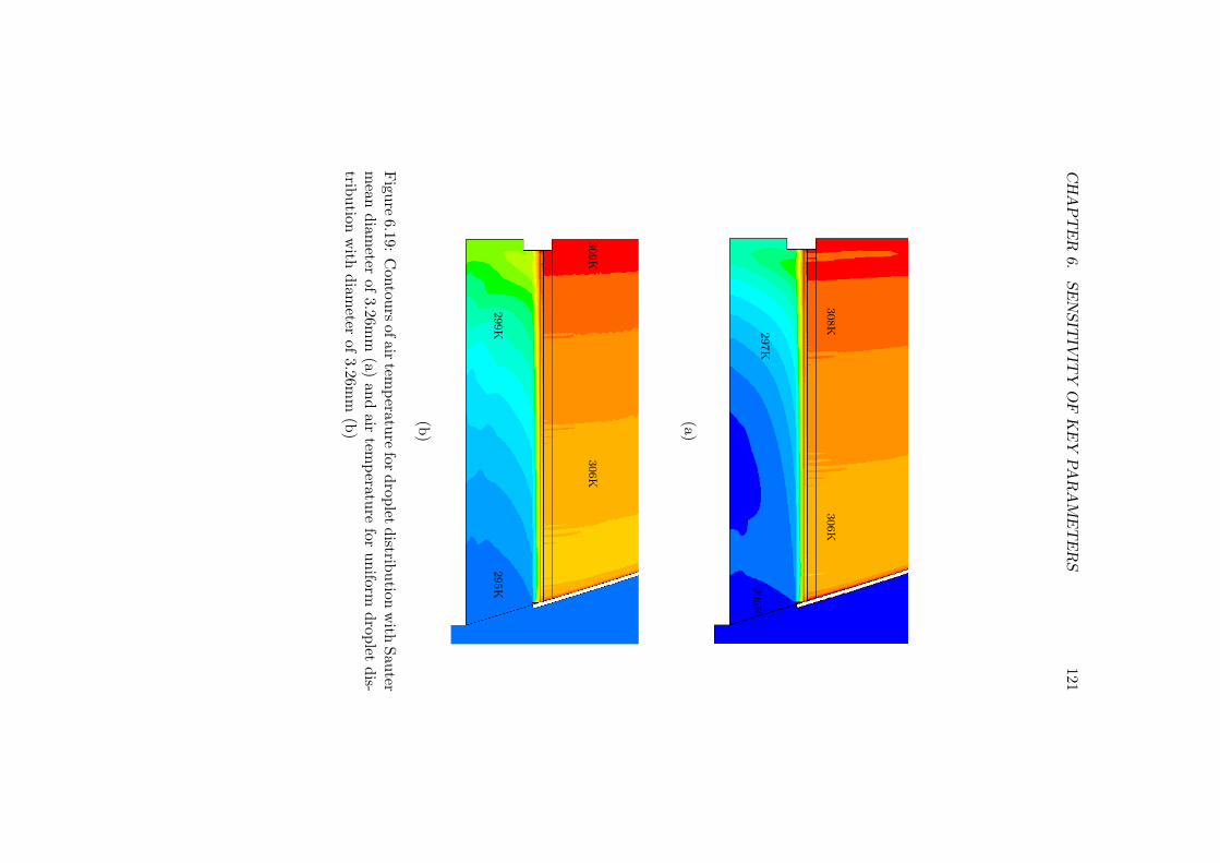
air in the rain zone. This is clearly seen in Fig. 6.19, in which the contours of
air temperature for the uniform droplet diameter case and the non-uniform
droplet distribution case are given. The cool region in the rain zone which
is observed in the case with the non-uniform droplet distribution, is absent
from the case with a uniform distribution. Additionally, the air temperature
in the rain zone clearly increases more uniformly across the tower for the
case with the uniform distribution. Overall, the proportion of heat and
mass transfer in the rain zone is slightly higher for the uniform distribution
as shown in Fig. 6.17 (a).
6.3 Conclusions
The results show that the air flow is quite uniform through the fill and
spray zones under the range of parameters considered in this study. The
flow appears to be strongly dominated by the resistance through the fill
region, including the spray zone and drift eliminators. Increasing the water
Figure 6.16: Radial profile of air mass flux in the fill (a), water temperature(b) and air temperature (c) with variable droplet diameter in the rain zone,with a tower inlet height of 8.577m, a water flow rate of 15000kg/s and afill depth of 1.0m
Figure 6.17: Radial profile of local water temperature drop per zone (a),cumulative heat transfer to air (b) and local cooling load (c) with variabledroplet diameter in the rain zone, with a tower inlet height of 8.577m, awater flow rate of 15000kg/s and a fill depth of 1.0m
Figure 6.18: Radial profile specific humidity with variable droplet diameterin the rain zone, with a tower inlet height of 8.577m, a water flow rate of15000kg/s and a fill depth of 1.0m
flow rate or reducing the inlet height, increases the resistance to radial flow
through the rain zone but the effect is relatively minor. Even at the smallest
fill depth tested, the air flow was quite uniform across the tower.
In spite of the uniform air flow, there can be considerable non-uniformity
of heat transfer and water outlet temperature across the tower, with a 6K
variation in water outlet temperature from the tower centre to the tower inlet
at reference conditions. This is shown to be largely due to the cooling load
in the rain zone and the radial air flow there. High radial non-uniformity of
heat transfer across the tower can be expected when the cooling load in the
rain zone is high. Such a situation can arise with small rain zone droplet
sizes, low fill depths, high water flow rates and to a lesser extent large inlet
heights. While ambient temperature and humidity can have a significant
influence on overall performance, the results here show that large changes
in these parameters have very little effect on the non-uniformity of heat
transfer across the tower.
The results show that the effect of inlet height on radial non-uniformity of
heat transfer is surprisingly very small. Reducing the inlet height increases
flow restriction in the tower and reduces heat transfer almost uniformly
across the tower. The inlet affected region has been shown to have a minor
effect on performance except when inlet heights are very low. The inlet
CH
AP
TE
R6.
SE
NSIT
IVIT
YO
FK
EY
PA
RA
ME
TE
RS
121
(a)
(b)
Figu
re6.19:
Con
tours
ofair
temperatu
refor
drop
letdistrib
ution
with
Sau
term
eandiam
eterof
3.26mm
(a)an
dair
temperatu
refor
uniform
drop
letdis-
tribution
with
diam
eterof
3.26mm
(b)
295K
299K
306K
309K
295K
297K
306K
308K
CHAPTER 6. SENSITIVITY OF KEY PARAMETERS 122
affected region was shown to cause an overall water temperature rise of only
0.14K at an inlet height of 4.977m. Furthermore, the influence of inlet height
on the relative cooling load in the rain zone was shown to be minor. These
are significant results for optimisation studies, where reducing the tower
inlet height is desirable as it reduces the water pumping power requirements.
This work demonstrates that the inlet height may be significantly reduced
without any additional design problems from re-circulation zones or non-
uniform flow through the fill.
The heat and mass transfer in the rain zone is shown to be significantly
different for the case where there is a non-uniform droplet distribution in the
rain zone and the case when there is a uniform droplet distribution at the
same Sauter mean diameter. This difference is because when there is a non-
uniform droplet distribution, the small droplets take different trajectories
from the larger droplets and undergo different rates of cooling.
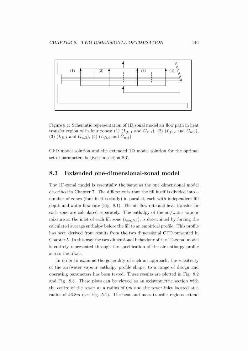
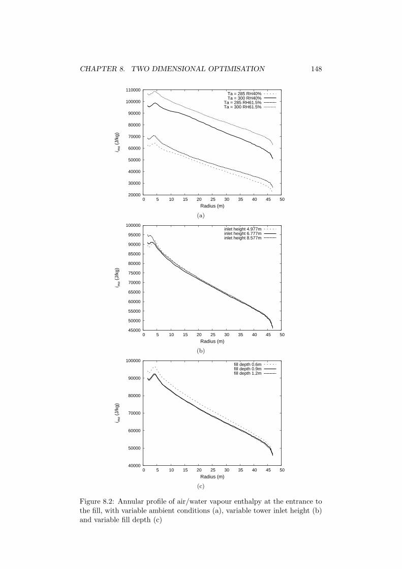
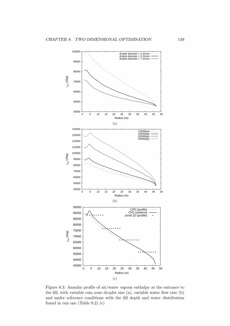
Chapter 7
One Dimensional Model
7.1 Introduction
In industry the majority of cooling tower design and optimisation is un-
dertaken using one dimensional models yet there is little work defining the
limitations of these models. As was shown in Chapter 6, there is a signif-
icant reduction in heat and mass transfer towards the centre of the tower
with a large gradient in water outlet temperature. The effects of these on
the predictions of simple one dimensional models are not well understood.
In this chapter, the numerical model presented in Chapter 5 is compared
with a one-dimensional model which does not solve for the flow field and
the predictions compared under a range of design conditions.
This chapter is arranged as follows. In section 7.2, previous work on the
development of the NDWCT one dimensional models has been reviewed.
In section 7.3, Kroger’s [1] one dimensional model has been described. In
section 7.5, the results of the comparison between the CFD model and the
one dimensional model are presented.
7.2 Previous work
Kroger’s [1] NDWCT modelling approach is the most detailed one dimen-
sional model in literature insofar as complete tower modelling is concerned.
Kroger and co-workers have contributed numerous publications on various
aspects of tower design and modelling [1, 12, 18–20, 32, 33, 52, 55, 61, 102,
104–108]. In Kroger’s model [1], the heat and mass transfer in the rain zone
123
CHAPTER 7. ONE DIMENSIONAL MODEL 124
is taken as a bulk averaged value in a similar manner to the fill. Hoffman
and Kroger [105] proposed the first semi-empirical transfer coefficient to ac-
count for the part cross-flow, part counterflow air/water flow in this region
which was later improved by de Villers and Kroger [20]. This is the only
correlation available in the literature and allows the rain zone to be treated
as an extension of the fill in the Merkel model. In essence, this method
assumes that the enthalpy of the air/water vapour mixture at the bottom of
the fill is uniform across the tower. For the spray zone, Kroger [1] correlated
Lowe and Christies’ spray data [7] in the format of the Merkel number (Eqn.
7.13).
The pressure losses that occur through the tower inlet, the contraction
into the tower fill, expansion losses out of the fill, and the losses as the
air stream exits the tower, are modelled in the same manner as the drift
eliminators, spray nozzles, tower supports and fill supports in the CFD
model. Much work has gone into developing empirical correlations for these
losses and understanding their interactions in a tower [1].
Lowe and Christie [7] used scale test models to determine the air velocity
profile across the tower and a loss coefficient for a number of shapes of
fill. The authors demonstrated that the resistance in an empty tower is
significant and is related to the ratio of the inlet height to the tower base
diameter. The authors stress the importance of ensuring an adequate inlet
height. The authors found that the loss coefficient of the system can be
found by adding the loss for the empty tower to the loss for the packing.
Terblanche and Kroger [107] conducted a model study and expressed
the inlet loss coefficients in terms of the height to diameter ratio and the
heat-exchanger/fill loss coefficient. The authors also showed that there is a
significant reduction in inlet losses when the lip of the shell inlet is rounded.
The author gives an empirical relation for the effective area as a function of
base diameter and inlet height. de Villers and Kroger [104] later advanced
the work with further experimental model studies and a CFD analysis. The
authors determined the influence of the rain zone on the inlet loss coefficient
and derived an empirical relationship.
Kroger [1] gives a complete compilation of available loss coefficients and
discussion on the topic.
CHAPTER 7. ONE DIMENSIONAL MODEL 125
7.3 One dimensional model
The one dimensional model presented here is based on Kroger’s [1] and
Kloppers’ [3] models. These models are obtained in the form of a heat
and mass transfer system coupled with a simple hydraulic flow calculation
where the system losses are represented with loss coefficients. These are
shown schematically in Fig. 7.1. Here the driving force for air flow is the
tower draft calculated simply as,
∆P = (ρ∞ − ρa,o)gHtower =n∑
i=1
KiρV 2
2, (7.1)
where the density ρ, the velocity V and the loss coefficients (Ki) are referred
to fill inlet conditions in the manner described in [1], thereby allowing the
coefficients to be summed. This simple model neglects an atmospheric lapse
rate but the CFD model used here has the same simplification so the models
are equivalent in this respect. The calculation of the air mass flow rate is
discussed in more detail in Appendix C.
The loss coefficients for the cooling tower shell supports, the water dis-
tribution piping network and the drift eliminators are the same as those em-
ployed in the CFD model in Chapter 5 (Kcts = 0.5, Kwdn = 0.5, Kfs = 0.5
and Kde = 3.5) as taken from [1]. In addition the tower inlet losses and
rain and spray zone losses are represented using the correlations described
in Kloppers thesis [3] and the citations therein. These are described in the
following sections.
The Merkel heat transfer method has been implemented here in the one
dimensional model, as the transfer characteristics for the rain and spray
zones are only available for the Merkel model and not the Poppe model.
The fill transfer coefficients for the Poppe model used in the CFD model are
derived from the same experimental data [3] as the Merkel transfer correla-
tions below (Eqns. 7.2-7.5). When implemented in the appropriate model
they produce the same result. The loss coefficients below (Eqns. 7.6 - 7.8)
are dissimilar to the Poppe loss coefficients in Chapter 5 as the air density
and fluid properties used to interpret the data are dependent on the heat
and mass transfer model used and so are different in each case [3].
CHAPTER 7. ONE DIMENSIONAL MODEL 126
1 2
3
4
Figure 7.1: Schematic representation of tower with flow resistance repre-sented as loss coefficients at locations: (1) = Kcts, (2) = Kct + Krz + Kfs,(3) = Kctc + Kfi + Kcte + Ksp + Kwdn + Kde and (4) = Kto
7.3.1 Fill transfer and loss coefficients
The following fill transfer coefficient correlations (Eqns. 7.2- 7.5) and loss
coefficient correlations (Eqns. 7.6 - 7.8) have been employed, all taken from
[3]. The correlations in Eqns. 7.2, 7.3 and 7.4 are used for fill depths of
0.6m, 0.9m and 1.2m respectively. In simulations of other fill depths, Eqn.
7.5 has been used.
Me0.6m
Lfi=
hmA
mwLfi
= 1.638988G0.282648w G0.682887
a
− 0.802755G0.560711w G0.644229
a (7.2)
Me0.9m
Lfi=
hmA
mwLfi
= 1.625618G0.091940w G0.702913
a
− 0.735958G0.376496w G0.6665399
a (7.3)
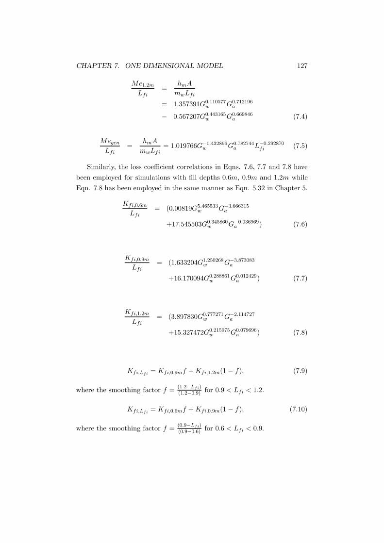
CHAPTER 7. ONE DIMENSIONAL MODEL 127
Me1.2m
Lfi=
hmA
mwLfi
= 1.357391G0.110577w G0.712196
a
− 0.567207G0.443165w G0.669846
a (7.4)
Megen
Lfi=
hmA
mwLfi= 1.019766G−0.432896
w G0.782744a L−0.292870
fi (7.5)
Similarly, the loss coefficient correlations in Eqns. 7.6, 7.7 and 7.8 have
been employed for simulations with fill depths 0.6m, 0.9m and 1.2m while
Eqn. 7.8 has been employed in the same manner as Eqn. 5.32 in Chapter 5.
Kfi,0.6m
Lfi= (0.00819G5.465533
w G−3.666315a
+17.545503G0.345860w G−0.036969
a ) (7.6)
Kfi,0.9m
Lfi= (1.633204G1.250268
w G−3.873083a
+16.170094G0.288861w G0.012429
a ) (7.7)
Kfi,1.2m
Lfi= (3.897830G0.777271
w G−2.114727a
+15.327472G0.215975w G0.079696
a ) (7.8)
Kfi,Lfi= Kfi,0.9mf + Kfi,1.2m(1 − f), (7.9)
where the smoothing factor f =(1.2−Lfi)(1.2−0.9) for 0.9 < Lfi < 1.2.
Kfi,Lfi= Kfi,0.6mf + Kfi,0.9m(1 − f), (7.10)
where the smoothing factor f =(0.9−Lfi)(0.9−0.6) for 0.6 < Lfi < 0.9.
CHAPTER 7. ONE DIMENSIONAL MODEL 128
7.3.2 Rain zone coefficients
The transfer coefficient and loss coefficient for the rain zone are given in
Figure 7.8: Incremental cooling range plotted against water flow rate withfill depth of 1.0m and inlet height of 8.577m
inlet heights.
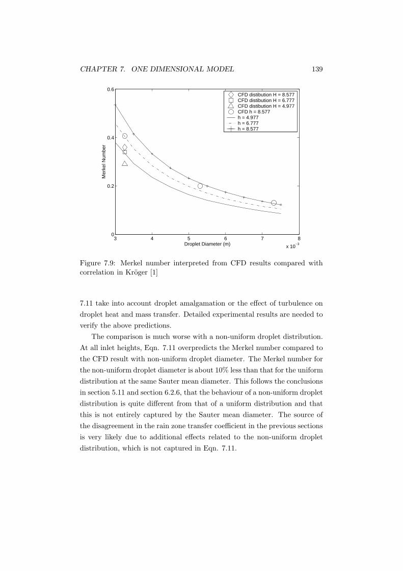
The effect of rain zone droplet size distribution has been examined by
plotting CFD results with uniform droplet size distribution in the rain zone
and with the droplet size distribution given in Table 5.3. The fluid flow
properties, the air-vapour velocity and other constants in Eqn. 7.11, have
been taken from the CFD model results with the droplet distribution at
each inlet height. The differences in these properties between the uniform
and non-uniform distributions are very small however and have no effect on
the comparisons in the plot.
The plot shows the agreement between Eqn. 7.11 and the CFD results
for uniform droplet diameters is very good at large droplet diameters, but
gets worse with decreasing droplet diameter. Both the CFD model and the
derivation of Eqn. 7.11 rely on general droplet empirical heat and mass
transfer correlations. The CFD model is a more detailed representation of
air flow and droplet trajectory integration however, which may be important.
In the derivation of Eqn 7.11, the droplet flow is assumed to have no effect
on the air flow. Also in the CFD model, the calculations are not performed
in isolation, but as part of the tower, so the air temperature/humidity and
water temperature vary across the tower. Neither the CFD model or Eqn.
CHAPTER 7. ONE DIMENSIONAL MODEL 139
3 4 5 6 7 8
x 10−3
0
0.2
0.4
0.6
Mer
kel N
umbe
r
Droplet Diameter (m)
CFD distibution H = 8.577CFD distibution H = 6.777CFD distibution H = 4.977CFD h = 8.577h = 4.977h = 6.777h = 8.577
Figure 7.9: Merkel number interpreted from CFD results compared withcorrelation in Kroger [1]
7.11 take into account droplet amalgamation or the effect of turbulence on
droplet heat and mass transfer. Detailed experimental results are needed to
verify the above predictions.
The comparison is much worse with a non-uniform droplet distribution.
At all inlet heights, Eqn. 7.11 overpredicts the Merkel number compared to
the CFD result with non-uniform droplet diameter. The Merkel number for
the non-uniform droplet diameter is about 10% less than that for the uniform
distribution at the same Sauter mean diameter. This follows the conclusions
in section 5.11 and section 6.2.6, that the behaviour of a non-uniform droplet
distribution is quite different from that of a uniform distribution and that
this is not entirely captured by the Sauter mean diameter. The source of
the disagreement in the rain zone transfer coefficient in the previous sections
is very likely due to additional effects related to the non-uniform droplet
distribution, which is not captured in Eqn. 7.11.
CHAPTER 7. ONE DIMENSIONAL MODEL 140
1 1.526
27
28
29
30
31
32
33
34
Wat
er O
utle
t Tem
pera
ture
( o C
)
Merkel Number
ima
= 50,000ima
= 70,000ima
= 90000
Figure 7.10: Water outlet temperature with Merkel number
7.7 Sensitivity of performance to Merkel number
In all the cases presented in this chapter, the predicted water outlet tem-
peratures for the CFD model and the one dimensional model are very close,
in spite of quite noticeable differences in the Merkel numbers. This is be-
cause heat transfer becomes less sensitive to Merkel number at higher Merkel
numbers. This is shown in Fig. 7.10 as a function of air inlet enthalpy.
ima = 50, 000J/Kg corresponds to approximately standard reference inlet
conditions and ima = 90, 000J/Kg, the air condition at the centre of the
tower (under reference conditions) where it has been significantly heated.
Increasing the Merkel number from 1.6 to 1.7 results in an increase in water
outlet temperature of about only 0.1K under standard tower design condi-
tions.
7.8 Poppe model comparison
Kloppers [3] compared the transfer characteristics for a particular fill found
using the Poppe approach and the Merkel approach. The author found that
across a broad range of ambient temperatures and humidities, the transfer
coefficient found using the Poppe approach was 7% larger than the one found
CHAPTER 7. ONE DIMENSIONAL MODEL 141
using the Merkel approach. Thus the author concluded that the transfer
correlations derived in Merkel format can be converted by increaseing them
by 7%. This rule of thumb has been used here to convert the rain zone
and spray zone transfer coefficient correlations in Eqn. 7.13 and Eqn. 7.11
into Poppe format. This has then been used to peform the comparison in
this chapter again using the Poppe model instead of the Merkel model. The
results of this comparison are very similar to those above so have not been
presented here.
7.9 Conclusion
A comparison has been made between a one dimensional NDWCT model
with Merkel heat transfer routine and a two dimensional CFD model. The
difference between the predictions of tower cooling range is very low, gener-
ally around 1-2%. This small difference appears to be due to a combination
of a slight difference in the prediction of the air flow rate and the corre-
lations for the transfer coefficient for the rain zone. The prediction of the
fill Merkel number by the one-dimensional method, appears to be slightly
conservative in all cases, but the difference is very small. In all cases the
rain zone Merkel number predicted by Eqn. 7.11 was greater than the CFD
result. The difference in the prediction of the tower draft is generally less
than 3%.
Additional tests were performed to determine the effect of the assump-
tions in the one dimensional model of uniform air flow through the fill and
averaged fill inlet air conditions. To make the test fair, the CFD results
were compared against the predictions of a one dimensional model in which
the air flow rate, and the rain and spray zone Merkel numbers were taken
from the CFD model. The difference between the tower range predicted by
the two models has been shown to be less than 0.4% in most cases. This
extraordinarily close comparison supports the one dimensional assumptions.
Furthermore, under the range of parameters tested here the difference be-
tween the CFD models predictions and those of the one dimensional models
remained fairly constant, suggesting that there is no particular area where
the flow becomes so skewed or non-uniform that the one dimensional model
predictions begin to fail. These results indicate that while there is significant
non-uniformity of heat transfer across the tower, the overall heat transfer is
CHAPTER 7. ONE DIMENSIONAL MODEL 142
essentially one-dimensional with respect to the variables tested.
For large rain zone droplet diameters, close agreement was found be-
tween the CFD model predictions of rain zone Merkel number and the semi-
empirical correlation in Eqn. 7.11. At small droplet diameters the agreement
is not as good and may indicate limitations of this correlation. Additionally,
the results with a non-uniform droplet distribution were found to compare
more poorly than those for the uniform distribution.
Chapter 8
Extendend One-Dimensional
Modelling and Optimisation
8.1 Introduction
The one dimensional model described in Chapter 7 is the type of model used
in NDWCT design and optimisation studies. The one dimensional nature of
the method places limitations on the range of design configurations that can
be considered. The fill depth and the water flow rate must be uniform across
the tower as non-uniform fill and water distributions cannot be resolved by
the one dimensional models. There is suggestion in literature that this is not
an optimal configuration and that other layouts should be considered [1].
In some instances designers have even opted to make ad-hoc attempts at
guessing the optimal fill layout and water distribution [1].
The purpose of this chapter is to attempt to quantify the improvement
in performance that can be achieved by using non-uniform fill and water
distribution. To this end an optimisation study has been undertaken using
the CFD model described in Chapter 5 and a new one dimensional model
which is described in this chapter. This new model is a simple extension
of the one dimensional design method described in Chapter 7. The exten-
sions allow two dimensional fill and water distribution configurations to be
simulated.
143
CHAPTER 8. TWO DIMENSIONAL OPTIMISATION 144
8.2 Previous work
A number of cooling tower economic and thermal optimisation studies have
appeared in literature, covering a range of cooling tower configurations. Lu
et al. [109] developed a model of a HVAC cooling system with a forced flow
cooling tower with variable fan speed and water load. They use a modified
genetic algorithm to find the optimal set points for fan and pump load to
minimise overall condenser loop power consumption. The authors found
that varying the fan speed and pump flow rate to match ambient conditions
saved as much as 50% at part load and 10% at full load in comparison to
the traditional system configurations. The savings were mostly due to the
savings in fan and pump power but also due to an increase in cooling tower
efficiency with a higher water supply temperature increasing the difference
between that and the ambient temperature enabling it to reject more heat.
Kintner-Meyer and Emery [110] conducted an optimisation study for a
chiller cooling system incorporating a forced draft cooling tower. The author
examined the relative contribution of the operating and capital costs under
a range of air and water temperatures. The author found that when consid-
ering the cooling tower on its own, there was significant room for reduction
in total cost but that when the entire system was considered including the
chiller plant, the cooling tower was a less significant part of the total cost.
The authors also noted that their study was only at full load and that at
part load the trade off between operating costs and capital costs is more
important.
Kloppers and Kroger [106] used their one-dimensional model of NDWCT
to find the optimal geometric dimensions of the tower that minimised its
cost over its entire operational life. The study considered a tower of similar
dimensions to the one in this study. The authors found the pumping cost
to be a significant factor in the model design. The optimal design reduced
the water distribution height and hence the tower inlet height significantly,
down to 4.9m. The authors noted that such a design also reduces the tower’s
susceptibility to cross-wind related performance penalties. Other changes
in the optimal model included a small decrease in tower diameter, small
decrease in tower height and a large increase in fill depth. The changes
reduced the cost of the tower by 18.7% over its useful life. This is the most
complete NDWCT optimisation study so far to appear in the literature.
CHAPTER 8. TWO DIMENSIONAL OPTIMISATION 145
Conradie et al. [19] performed a similar study to determine the optimal
design parameters for a dry cooling tower. They examined in detail the
costs of the entire plant and were able to reduce the cost of the cooling
system through modification of the tower’s geometry and heat exchanger
design.
Radosavljevic’s [5] study into NDWCTs has aspects that are similar to
the study considered here. The author used a two-dimensional axisymmetric
numerical model to run a parametric study to determine the effect of chang-
ing the fill shape and water distribution. The author found that removing a
small amount of fill from the centre of the tower, while maintaining the same
overall fill volume, improved the tower performance, but by only 0.03K. A
very limited range of fill shapes were tested with no optimisation study.
In some instances designers have opted to counter the radial heat and
mass transfer profiles and improve tower performance by having a fill of
variable depth across the tower [1]. There has been no formal investigation
to determine the optimal fill layout and water distribution across the tower
appearing in the literature to date.
Here an attempt is made to quantify the improvement possible by vary-
ing both the water flow rate and fill depth across the tower. An evolutionary
optimisation routine has been implemented here. A number of recent pub-
lications have employed such techniques for shape optimisation [111–114].
Such algorithms operate by evaluating a large number of points in the so-
lution space, typically above 2000. It is therefore essential that the model
or fitness function allows rapid evaluation of these points. While a two di-
mensional CFD model has a high resolution it takes orders of magnitude
longer to solve than a simple one dimensional model so is unsuited for use
in an optimisation study. Here instead, an extended one dimensional model
is developed as an attempt to retain partial two dimensional resolution in
the fill region, without the time penalty of a full Navier Stokes solver. This
extended model has been termed a ’1D-zonal’ model and is simply a one-
dimensional model which has semi-two dimensional capability in the fill and
spray zone regions.
This chapter is laid out as follows. In sections 8.3 and 8.4, an extended
one dimensional model is presented. The optimisation problem and the
evolutionary optimisation procedure are described in section 8.5 and section
8.6. The results of the optimisation together with a comparison between the
CHAPTER 8. TWO DIMENSIONAL OPTIMISATION 146
6
66 6 6 6(1) (2) (3) (4)
Figure 8.1: Schematic representation of 1D zonal model air flow path in heattransfer region with four zones; (1) (Lfi,1 and Gw,1), (2) (Lfi,2 and Gw,2),(3) (Lfi,3 and Gw,3), (4) (Lfi,4 and Gw,4)
CFD model solution and the extended 1D model solution for the optimal
set of parameters is given in section 8.7.
8.3 Extended one-dimensional-zonal model
The 1D-zonal model is essentially the same as the one dimensional model
described in Chapter 7. The difference is that the fill itself is divided into a
number of zones (four in this study) in parallel, each with independent fill
depth and water flow rate (Fig. 8.1). The air flow rate and heat transfer for
each zone are calculated separately. The enthalpy of the air/water vapour
mixture at the inlet of each fill zone (ima,fi,i), is determined by forcing the
calculated average enthalpy before the fill to an empirical profile. This profile
has been derived from results from the two dimensional CFD presented in
Chapter 5. In this way the two dimensional behaviour of the 1D-zonal model
is entirely represented through the specification of the air enthalpy profile
across the tower.
In order to examine the generality of such an approach, the sensitivity
of the air/water vapour enthalpy profile shape, to a range of design and
operating parameters has been tested. These results are plotted in Fig. 8.2
and Fig. 8.3. These plots can be viewed as an axisymmetric section with
the centre of the tower at a radius of 0m and the tower inlet located at a
radius of 46.8m (see Fig. 5.1). The heat and mass transfer regions extend
CHAPTER 8. TWO DIMENSIONAL OPTIMISATION 147
from the tower inlet to the causeway at a radius of 1.4m. Unless otherwise
stated the fill depth is 1.0m, the water flow rate 15,000kg/s, the droplets
in the rain zone follow the distribution given in Table 5.3, the tower inlet
height is 8.577m and the ambient air is at 295K and 55% relative humidity.
The air/water vapour mixture enthalpy at the fill inlet has been calculated
Figure 8.3: Annular profile of air/water vapour enthalpy at the entrance tothe fill, with variable rain zone droplet size (a), variable water flow rate (b)and under reference conditions with the fill depth and water distributionfound in run one (Table 8.2) (c)
CHAPTER 8. TWO DIMENSIONAL OPTIMISATION 150
8.4 Model procedure
The 1D-zonal model solution procedure is described in Fig. 8.4. It is very
similar to one dimensional model in Chapter 7, where the Merkel model
is used for the heat and mass transfer and the simple draft equation is
solved for the air flow (Eqn. 7.1). The additional modelling assumptions
are summarised as follows:
1. The pressure drop is uniform across all fill sections.
2. The airflow through the fill is assumed to remain fairly uniform, such
that the rain zone transfer coefficient (Eqn. 7.11) and loss coefficient
(Eqn. 7.12) and the loss coefficients for the tower inlet (Eqn. 7.15)
taken from Kroger [1] can be applied.
3. The enthalpy profile specified at the fill inlet is assumed to remain
constant despite changes to fill shape and water distribution.
4. The loss coefficient for the rain zone affects all the fill sections equally.
The heat and mass transfer process is split between the rain zone and
the fill zones. The average air/water vapour enthalpy leaving the rain zone
(ima,rz,o) is found by solving the Merkel model for the rain zone (Table 2.3),
between the average water temperature leaving the fill (Tw,rz,i) and the tower
water outlet temperature (Tw,rz,o). The average air/water vapour enthalpy
leaving the rain zone, ima,rz,o, and entering each fill zone, j, is determined
by Eqn. 8.3,
ijma,fi,i = i′jma,fi,i
ima,rz,oma,total
∑kj=1
[i′jma,fi,i · m
ja
] , (8.3)
where mja is the dry air mass flow rate in each fill zone, ma,total is the
total dry air mass flow rate in the tower and i′jma,fi,i is the average enthalpy
entering each fill zone under reference conditions, calculated using Eqn. 8.2.
In this way the average enthalpy entering the fill is still ima,rz,o, but the
profile now has the same shape as Eqn. 8.2. The entire process (given in
Fig. 8.4) is very iterative, with the guessed and calculated values for ima,rz,o,
Tw,o and ma required to be within the tolerances specified, δma , δMe, δima,rz .
In this study, δMe = 5 × 10⁻⁵, δma = 1 × 10⁻¹kg/s, δima,rz = 10J/Kg and
Crelax = 0.8.
CHAPTER 8. TWO DIMENSIONAL OPTIMISATION 151
1 Initialisation of variables: specify mjw, Lj
fi, Ta,i Tw,i,δma , δMe, δima,rz
2 Guess T jw,fi,o, ima,rz,o and Ta,o
3 Estimate ma and mja to find Ktot, Kj
fi
4 Solve tower draft equation (Eqn. 7.1) using the guessed Ta,o,to find ma (see Appendix C)
5 c = 1;6 While : δc
ma> δma
7 c = c + 1; n = 08 While : δn
ima,rz> δima,rz
9 n = n + 110 inma,rz,o = in−1
ma,rz,o
11 For j = 1,2...k
12 Calculate ijma,fi,i using Eqn. 8.3 and inma,rz,o
13 Calculate Mejfi and Mesp,i using Eqn. 7.5 and Eqn. 7.13
14 Solve the Merkel equations for fill zone j, using the
procedure in Table 2.3 (b),to find T jw,fi,o
15 Find the average water temperature entering the rain zone,
Tw,rz,i =∑k
j=1 T jw,fi,om
jw/mw
16 Calculate Merz using Eqn. 7.1117 Solve the Merkel equations, for the rain zone region, using
the procedure in Table 2.3 (b), to find Tw,rz,o and inma,rz,o
18 δnima,rz
= inma,rz,o − in−1ma,rz,o
19 Calculate Ta,fi,o from bulk average ima,fi,o, using Eqn. B.1720 m = 0 , m′m
a = mca
21 While δ′mma> δma
22 m = m + 123 m′m
a = m′m−1a + Crelax(m
′ma − m′m−1
a )
24 Calculate loss coefficient for each fill zone Kjfi,z, using Eqn. 7.9
25 Calculate the loss coefficient for all components in thetower except the fill: Knfi (see Appendix C)
26 Calculate pressure head available ∆Ptot = (ρ∞ − ρa,o)gHtower
i.e. (Eqn. 7.1)27 Calculate pressure drop across components except for the fill
∆Pother = KnfiρV 2
2 (see Appendix C)28 Calculate pressure drop across the fill ∆Pfill = ∆Ptot − ∆Pnfi
29 Calculate air flow rate mja across the fill zones assuming
equal pressure drop ( ∆Pfill) across each zone
30 Sum to find total air flow in the tower m′m+1a =
∑kj=1 mj
a
31 δ′mma= m′m+1
a − m′ma
32 mc+1a = m′m+1
a
33 δcma
= mc+1a − cn
a
34 END
Figure 8.4: 1D-zonal model solver procedure
CHAPTER 8. TWO DIMENSIONAL OPTIMISATION 152
8.5 Problem description
Here we have attempted to optimise a standard NDWCT fill and water
distribution across the tower such that the fill and water volume remain
constant. The 1D-zonal model has been divided into four sections with the
fill depth and water distribution uniform across each of the sections. The
objective function to be maximised is the tower range (Trange = Twi −Two).
The search space is bounded by the following constraints:
The water flow rate for Gw,1 to Gw,3 can vary between 2.0 < Gw < 2.3.
The fill depth Lfi,1 to Lfi,3 can range between 0.6 < Lfi < 1.2. The
constraint for constant total fill volume is enforced through Lfi,4 such that
Lfi,4 =
(Vfill,tot − [
∑3n=1 Lfi,n · Af,n]
)/Af,4, where Vfill,tot is the total fill
volume such that the average fill depth is 1.0m. The total water flow rate
Gw,tot (15,000kg/s) is enforced through Gw,4 such that Gw,4 =
(15, 000 −
[∑3
n=1 Gw,n · Af,n]
)/Af,4.
8.6 Evolutionary algorithm procedure
The optimisation procedure implemented here is an evolutionary algorithm,
similar to that described in Michalewicz [115]. These routines have been
shown to be robust and reliable in conditions where traditional methods
can fail to find a global optimum [115, 116]. They have been widely studied
and implemented in a variety of difficult engineering problems [111–114].
The basic operation of this algorithm is presented here for completeness.
An ’individual’ is a collated string of system variables. Each variable is
represented using floating point numbers.
The algorithm proceeds as depicted in Fig. 8.5, where an initial pop-
ulation undergoes mutation, cross-over and selection operations until the
termination conditions are reached. An elitist strategy is implemented here
where the best individual from each generation is retained and is used to
replace the least fit individual. This allows high mutation and crossover
rates to be employed without fear of losing the good candidates [116]. The
operator probabilities and other algorithm constants are contained in Table
8.1.
CHAPTER 8. TWO DIMENSIONAL OPTIMISATION 153
1) Begin2) Initialise population3) Evaluate objective function4) Store best individual5) Selection: generate a
new mating population withtournament selection
6) Apply cross-over andmutation operators
7) Store current population8) If generation < max
generations goto (3)
9) End
Figure 8.5: Schematic representation of the evolutionary algorithm proce-dure
8.6.1 Selection operators
Here the tournament selection method is implemented. These selection pro-
cedures do not use the fitness values directly in selection, only the relative
rank of the individuals [115]. In this method, individuals compete against
each other in many small ’tournaments’, where the most fit member is se-
lected for the new population. The method proceeds as follows: k individuals
are randomly chosen from the old population. The most fit individual from
this subset is selected for the next generation. This procedure is repeated
until the new population is filled. The larger the value of k, the higher the
selection pressure.
8.6.2 Mutation operators
Three floating point mutation operators were employed for the optimi-
sation study. These are taken from Michalewicz [115]. In all cases, a
single candidate X ′ = (x1, ..., x′
j , ..., xn) is created from a single parent
X = (x1, ..., xj , ..., xn) by randomly selecting and replacing the element xj
of a parent X with x′
j where, j ∈ (1, ..., n) and x′
j lies within the feasible
range 〈Lj , Uj〉. The method of generating x′
j is unique to each mutation
operator.
CHAPTER 8. TWO DIMENSIONAL OPTIMISATION 154
Table 8.1: Evolutionary algorithm operator probabilities and parametersOperator Value
Probability of non-uniform mutation 0.20Shape parameter (b) 3.0
Probability of uniform mutation 0.05Probability of heuristic crossover 0.05
Probability of arithmetic crossover 0.05Probability of simple crossover 0.05
Population 30Max no. of generations 200Tournament size (k) 2
Heuristic cross over attempts (w) 5
Uniform mutation
This operator sets x′
j equal to a random number with a uniform probability
distribution in the feasible range 〈Lj , Uj〉. The operator is important early
in the search as it covers the search space with uniform probability.
Non-uniform mutation
This operator is a function of generation, where the allowable mutation gets
smaller with each succeeding generation. The operator randomly determines
if the selected variable, x′
j, should be mutated in the direction of its upper or
lower boundary such that x′
j = xj+(Uj−xj)∗f(t) or x′
j = xj−(xj−Lj)∗f(t),
if a uniform random number, r1, is < 0.5 or ≥ 0.5 respectively. The shape
function is f(t) = r2 · (1 − tTmax
)b, where Tmax is the maximum number of
generations, t is the current generation, b is the shape parameter (=3) and
r1 and r2 are random numbers between 0 and 1.
8.6.3 Crossover operators
Three crossover operators are employed in this study. These are taken from
[115].
Simple crossover
Two parent individuals X = (x1, ..., xn) and Y = (y1, ..., yn), are cut at
the jth position and rejoined here to create two new individuals X ′ =
CHAPTER 8. TWO DIMENSIONAL OPTIMISATION 155
(x1, ..., xj , yj+1..., yn) and Y ′ = (y1, ..., yj , xj+1, ..., xn).
Heuristic crossover
This operator uses fitness information to create a single new individual X ′
from two parents X and Y . The new individual is X ′ = r · (X − Y ) + X,
where X has a higher fitness than Y (for maximisation problems) and r
is a random number between 0 and 1. This may fall outside the feasible
solution space so if after w attempts no feasible solution is produced, the
operation is terminated and no new offspring is created. The operators
unique contribution is that it uses fitness information to select a promising
search direction.
Arithmetic crossover
This operator produces two new individuals X ′ and Y ′ from two parents X
and Y with X ′ = r · X + (1 − r)Y and Y ′ = r · Y + (1 − r)X, where r is a
random number between 0 and 1. This allows the linear combination of two
parents with a random amount of mixing.
8.7 Results and discussion
The optimisation routine has been run four times as it is a stochastic process
with results slightly different each time (Table 8.2). The centre variables
Lfi,1 and Gw,1 affect the solution very weakly so they have some variation
in the final solution. The axisymmetric geometry means the fill volume per
unit radius increases with radius, so changes in the tower centre have less of
an effect on the overall tower performance.
The difference in water outlet temperatures predicted by the CFD model
and the 1D zonal method is approximately 0.04K. The improvement of the
fill depth and water distribution profile can be compared against a uniform
fill and water distribution in row 5 of Table 8.2. The improvements predicted
by the two models are identical in all but one case, supporting the models
equivalence.
The air enthalpy at the entrance to the fill is slightly over-predicted by
the 1D-zonal model (Fig. 8.3 (c)) compared to the CFD model. This follows
the conclusions presented in Chapter 7, that the rain zone transfer coefficient
CH
AP
TE
R8.
TW
OD
IME
NSIO
NA
LO
PT
IMIS
AT
ION
156
Table 8.2: Optimal set of design parameters with tower rangeas computed by the 1D zonal method and the CFD methodFill depth (m) Water mass flux (kg/s/m2) Tower Range (K)
given in [1] is over-predicted for non-uniform droplet size distributions. The
air enthalpy profile predicted by the CFD model under the uniform case is
quite close to the CFD results with the fill and water distribution from run
one. This supports the original assumptions that for small changes in fill
depth and water flow rate the ima profile changes very little.
A comparison of the CFD and the 1D zonal results for the parameters
in run one show very good agreement (Fig. 8.6 - Fig. 8.7 and Table 8.2).
The 1D-zonal model predicts air flow within 5% of the CFD value (Fig. 8.6
(a)). The water temperature below the fill follows the same trend as the
CFD method in each of the four zones (Fig. 8.6 (b)). Overall the 1D-zonal
model predicts the heat transfer and airflow distribution well.
On the same plots, a comparison is made between the CFD results of a
uniform fill and water distribution profile. The lower fill depth in the tower
centre has the effect of increasing the air flow there and reducing it in the
outer region. The actual overall heat transfer to the air from the tower inlet
to the fill outlet changes very little, although the air temperature at the fill
outlet is reduced slightly with the shallower fill and higher air flow here.
The overall improvement in performance with the optimal profile has
been shown to be very marginal, with an increase in water range of only
0.04K. With a fixed fill volume, a big decrease in fill depth at the tower
centre only allows a relatively small increase in fill depth in the tower’s outer
regions. Additionally, this study shows that Lowe and Christie [7] were not
entirely correct that the air has ”already been heated nearly to capacity” in
the centre of the tower. Figs. 6.1 - 6.18 show that except at very high water
flow rates, the cooling in the centre of the tower is still significant. Entirely
sacrificing this cooling for the outer regions is not optimal.
As discussed previously, since the non-uniformity is specified through
the ima profile, we can draw some conclusions as to the generality of the
result. The ima profiles are independent of tower inlet height, fill depth
and ambient air temperature and humidity (see Fig. 8.2 and 8.3) so the
results here should apply over these conditions. The optimisation is likely
to be more effective at very high water flow rates as indicated by the large
variation in ima across the tower in Fig. 8.3 for mw = 30, 000 kg/s. For the
range of variables tested here however, the results show that two-dimensional
optimisation is unnecessary and a uniform fill and water distribution profile
is adequate.
CHAPTER 8. TWO DIMENSIONAL OPTIMISATION 158
0
0.2
0.4
0.6
0.8
1
1.2
1.4
1.6
1.8
2
0 5 10 15 20 25 30 35 40 45 50
Dry
Air
Mas
s F
ux (
kg/s
/m2 )
Radius
1D zonalCFD (profile)
CFD (uniform)
(a)
296
298
300
302
304
306
308
310
312
0 5 10 15 20 25 30 35 40 45 50
Wat
er T
empe
ratu
re (
K)
Radius (m)
Fill Water Inlet
Fill Water Outlet
Basin
CFD (profile)1D zonal
(b)
Figure 8.6: A comparison of the annular profile of the air mass flux in thefill (a) and water temperature through the tower (b) in both the 1D zonaland CFD models with the fill depth and water distribution profile from runone in Table 8.2 and the CFD model with a uniform profile
CHAPTER 8. TWO DIMENSIONAL OPTIMISATION 159
294
296
298
300
302
304
306
308
310
0 5 10 15 20 25 30 35 40 45 50
Air
Tem
pera
ture
(K
)
Radius (m)
Fill Air Inlet
Fill Air outlet
CFD (profile)CFD (uniform)
(a)
0
20
40
60
80
100
120
140
160
0 5 10 15 20 25 30 35 40 45 50
Ga
(i ma,
o -
i ma,
i) (k
W/m
2 )
Radius (m)
Fill Air Outlet
Fill Air Inlet
CFD (profile)CFD (uniform)
(b)
Figure 8.7: A comparison between air temperature (a) and heat transferto air through the fill (b) in the CFD model with a uniform fill depth andwater distribution and that with the profile from run one in Table 8.2
CHAPTER 8. TWO DIMENSIONAL OPTIMISATION 160
8.8 Conclusions
A simple extension to a one dimensional model has been proposed allow-
ing reduced-two dimensional modelling of a NDWCT. The model has been
successfully coupled with a robust optimisation routine to determine the
optimal fill profile and water distribution across the tower. The optimal
profile differs from a uniform profile, with greater water flow rate and fill
depth located in the outer region of the tower near the inlet. The potential
improvement in performance has been shown to be very marginal.
The axisymmetric shape of the tower means that reducing the fill depth
in the centre of the tower allows only a small increase in fill depth near the
outer region, and since cooling in the centre is still effective this reduces the
performance here. The work demonstrates that the centre of the tower is
far from a ’dead zone’ with no cooling and that significantly reducing the
fill depth here is not optimal. In addition, the modified fill and water distri-
bution significantly effect the air-flow in the tower, reducing air flow to the
more effective regions near the tower inlet. Thus the highly coupled nature
of the flow in the tower limits our ability to make significant improvements in
tower performance, with small changes in water and fill depth distribution.
The results in this study indicate that little improvement can be expected
from annularly varying fill depth and water flow rate and that unless it is
done carefully, performance may actually be reduced.
Chapter 9
Conclusions
9.1 Study results and objectives
The aims of this study as stated in Chapter 1 are repeated below:
1. Develop a CFD model of a NDWCT and further understanding of the
heat and mass transfer processes in the tower and how they are coupled
with the air flow field. Provide designers with immediate conclusions
on how tower performance is related to key design parameters.
2. Examine a detailed one dimensional model and compare performance
predictions with a multi dimensional CFD model computing the air
flow field under a range of design parameters.
3. Quantify the improvement possible with multi-dimensional optimisa-
tion by optimising the fill depth and water distribution radially across
the tower.
Objective one
An axisymmetric numerical model of a NDWCT has been developed within
FLUENT. The model is based on a NDWCT at Mt. Piper Power Station, in
Lithgow NSW and operated by Delta Electricity. The geometry and design
parameters have been based on those of the reference tower but in some
cases, the performance characteristics of key components were unknown.
The fill characteristics have been based on experimental data and empirical
correlations published in Kloppers and Kroger’s work [3, 61, 102]. The
161
CHAPTER 9. CONCLUSIONS 162
characteristics of the rain zone droplet distribution and flow were taken
from Kroger [1] and those for the spray zone from Bellagamba [101].
This model is an advance on previous models, with the generality of the
empirical correlations used and the detail to which condensation is repre-
sented, improved over previous efforts. The water flow in the rain and spray
zones has been modelled in more detail with two-dimensional Lagrangian
particle motion and the droplet distribution in the rain zone represented.
The assumption of uniform droplet diameter and vertical droplet flow used
in previous studies has been shown in this study to give misleading results.
The model has been partially validated against reference manufacturers cool-
ing tower performance data, comparing the cooling range over a range of
ambient air temperatures and humidity levels.
A study was conducted testing the influence of the following key design
and operating parameters; the fill depth, tower inlet height, water flow rate,
ambient air temperature and humidity and the initial water droplet diameter
and distribution in the rain zone. In particular, the radial non-uniformity of
heat transfer and air flow due to local geometric effects and overall gradients
in air temperature/humidity and flow rate are examined. The results show
that with the exception of a small inlet effected region, the air flow is quite
uniform through the fill and spray zones under the range of parameters
considered in this study. The flow appears to be strongly dominated by
the resistance through the fill region, including the spray zone and drift
eliminators. Increasing the water flow rate or reducing the inlet height,
increases the resistance to radial flow through the rain zone but the effect
is relatively minor. Even at the smallest fill depth tested (Lfi = 0.6m), the
air flow was quite uniform across the tower. The inlet effected region does
not become significant even at the lowest inlet height tested (hi = 4.977m).
In no cases was any recirculation zone observed in the fill.
In spite of the uniform air flow, there can be considerable non-uniformity
of heat transfer and water outlet temperature across the tower. Under refer-
ence conditions, there is a 6K variation in water outlet temperature from the
tower centre to the tower inlet. This is shown to be due to the cooling load
in the rain zone and the radial air flow there. High radial non-uniformity of
heat transfer across the tower can be expected when the cooling load in the
rain zone is high. Such a situation can arise with small rain zone droplet
sizes, low fill depths and high water flow rates.
CHAPTER 9. CONCLUSIONS 163
The results show that the effect of inlet height on radial non-uniformity of
heat transfer is surprisingly very small. Reducing the inlet height increases
flow restriction in the tower and reduces heat transfer almost uniformly
across the tower. The inlet affected region has been shown to have a minor
effect on performance except when inlet heights are very low. The inlet
affected region was shown to cause an overall water temperature rise of only
0.14K at an inlet height of 4.977m. Furthermore, the influence of inlet height
on the relative cooling load in the rain zone was shown to be minor. These
are significant results for optimisation studies, where reducing the tower
inlet height is desirable as it reduces the water pumping power requirements.
This work demonstrates that the inlet height may be significantly reduced
without any additional design problems from re-circulation zones or non-
uniform flow through the fill.
When the water mass flux is greater than 3.3kg/s/m2, the cooling in the
centre of the tower starts to become less effective with the air at the centre
of the tower close to the water temperature and saturated. Under reference
conditions of 2.21kg/s/m2 , the centre of the tower still contributes to total
cooling.
While ambient temperature and humidity can have a significant influence
on overall performance, the results here show that large changes in these
parameters have very little effect on the non-uniformity of heat transfer
across the tower. Similarly, with a uniform fill depth of greater than 1m,
the non-uniformity of cooling across the tower changes very little.
The heat and mass transfer in the rain zone is sensitive to both the
droplet size and droplet size distribution in the rain zone. The heat and mass
transfer is more complicated with a non-uniform distribution than a uniform
distribution at the same Sauter mean diameter. With a non-uniform droplet
size distribution, the rates of cooling among the droplets are different and
they follow different trajectories. This leads to the situation where the small
droplets can be quickly cooled to below the air temperature by evaporation
and effectively cool the incoming air.
Objective two
A comparison has been made between a one dimensional NDWCT model
with Merkel heat transfer routine and the two dimensional CFD model. The
main point of interest here, is to determine if the non-uniform cooling across
CHAPTER 9. CONCLUSIONS 164
the tower leads to poor one-dimensional model performance predictions.
The two models were compared across a wide range of design and operating
variables.
In all cases, the difference between the predictions of tower cooling range
is very low, generally around 1-2%. The small difference appears to be
mostly due to a combination of a slight difference in the prediction of the
air flow rate and the correlations for the transfer coefficient for the rain zone
used in the one dimensional model. The difference in the prediction of the
tower draft is generally less than 3%.
A comparison of the CFD results with a one dimensional method using
the CFD draft and CFD transfer coefficients for the rain zone and spray
zone was used to test the one dimensional assumptions of uniform air flow
through the fill and averaged inlet air conditions. The difference between
the tower range predicted by the two models has been shown to be less than
0.4% in most cases. Furthermore, under the range of parameters tested
here the difference between the CFD model predictions and those of the
one dimensional models remained fairly constant suggesting that there is no
particular area where the flow becomes so skewed or non-uniform that the
one dimensional model predictions begin to fail. Even at extreme values
of inlet height and fill depth, the models work well, and other secondary
effects, such as the inlet effected region or the radial gradient of heat and
mass transfer, do not effect the overall accuracy.
An additional point of interest is a comparison between the CFD model
predictions of rain zone Merkel number and the semi-empirical correlation
in Eqn. 7.11. The agreement is very good for large droplet diameters, but
gets worse with decreasing diameter. The results with a non-uniform droplet
distribution were found to compare more poorly than those for the uniform
distribution. A portion of the discrepancy between the CFD model and the
one-dimensional model can therefore be attributed to the differences in the
prediction of the rain zone Merkel number.
The conclusion of this work is that the assumption of bulk averaged heat
and mass transfer implicit in the one-dimensional models does appear to be
a good approximation. The prediction of tower range is helped by the fact
that at high Merkel numbers, the water outlet temperature becomes less
sensitive to a change in Merkel number.
CHAPTER 9. CONCLUSIONS 165
Objective three
The high non-uniformity of heat transfer and the large gradient of air tem-
perature and humidity across the cooling tower raise the possibility of radi-
ally varying the water flow rate and fill depth to improve tower performance.
A simple extension to a one dimensional model has been proposed allow-
ing reduced-two dimensional modelling of a NDWCT. This model has been
compared with the axisymmetric CFD model and found to perform well,
with considerable computational savings. The model has been successfully
coupled with a robust optimisation routine to determine the optimal fill
profile and water distribution across the tower. The optimal profile differs
considerably from the uniform profile, however the potential improvement
in performance has been shown to be very marginal.
The reason for this is as follows. Firstly, with a fixed fill volume, a
big decrease in fill depth at the tower centre only allows a relatively small
increase in fill depth in the tower’s outer regions because of the axisymmetric
geometry. Secondly, this study shows that Lowe and Christie [7] were not
entirely correct in their assumption that the air has ”already been heated
nearly to capacity” in the centre of the tower. Except at very high water
flow rates, the cooling in the centre of the tower is still significant. Entirely
sacrificing this cooling for the outer regions is not optimal. Re-designing
the NDWCT to improve this region is not effective and any ad hoc design
modification would be unlikely to improve tower cooling.
9.2 Closing discussion and significant results
This work has demonstrated that a NDWCT model can be developed within
a CFD code such as FLUENT and provided a simple methodology for rep-
resenting the combined heat and mass transfer processes in a manner equiv-
alent to the Poppe model. In the course of the study, several unexpected
results have been obtained. Contrary to suggestion in literature, air flow
is quite uniform across a NDCWT. Heat and mass transfer is non-uniform
across the tower but on average is one dimensional with respect to all de-
sign parameters tested. While heat transfer in the centre of the tower is
clearly less effective, re-designing the fill layout or water distribution to
achieve more uniform heat and mass transfer is not effective and should be
approached with caution. These results, while not dramatic, are important
CHAPTER 9. CONCLUSIONS 166
and end some uncertainty in the literature.
In addition, the work has highlighted several interesting results with
respect to heat and mass transfer in the rain zone. This study has shown
the importance of the rain zone in overall understanding of the heat and
mass transfer in a NDWCT. The radial heat and mass transfer to the air
through the rain zone is the primary reason for the variation in water outlet
temperature across the tower. In addition, the study has shown that the
droplet distribution in the rain zone is important and needs to be accounted
for. Approximating the droplet distribution in the rain zone, as uniform,
at the same Sauter mean diameter may give misleading results and should
be taken with care, both in numerical models and with development of
empirical correlations.
A part of the objective of this study is to provide designers with in-
sights into the flow within a typical NDWCT and how cooling may be im-
proved. With respect to multi-dimensional optimisation, this study has
clearly demonstrated that radial variation in water flow rate and fill depth
provides only a marginal improvement in tower cooling. With respect to
tower design with uniform fill depth and water distribution, this study pro-
vides some immediate results that may be used as a check on design changes
suggested by results from a one-dimensional model. For example, Kloppers
and Kroger [106] used a one dimensional model to optimise a NDWCT to
minimise the total economic cost of the tower over its life. The authors
found that the cost was minimised with an increased fill depth and a very
low inlet height, which reduces the elevation at which the water distribu-
tion nozzles are located and hence reducing pumping costs. This work has
demonstrated that reducing the tower inlet height has relatively little effect
on the overall radial heat and mass transfer or the local inlet effects. The
inlet effected region was shown to cause an overall water temperature rise
of only 0.14K at an inlet height of 4.977m. Furthermore, as the fill depth
is increased, the air-flow profile in the fill becomes more uniform and there
is little effect on the radial heat transfer distribution as the rain zone is
unaffected. Proof that such a design would be feasible in a two dimensional
study is valuable. Even at the smallest inlet height tested in this thesis,
the inlet effected region was shown not to be problematic and overall the
tower was still well modelled with a one dimensional model. Under the wide
range of parameters investigated in this model, no re-circulation zone was
CHAPTER 9. CONCLUSIONS 167
observed under the fill at the tower inlet.
9.3 Recommendations for further work
A cooling system such as a NDWCT is the sum of many individual compo-
nents including the fill, drift eliminators and spray nozzles. Continued design
optimisation and understanding of the performance of these components is
required.
Validation of NDWCT CFD models is at present very difficult, limiting
the confidence with which they can be applied. Full scale experimental
results are required together with details of the tower components and their
characteristics.
Very few studies have been devoted to understanding of the rain zone and
the extent to which performance can be improved in this region. Decreasing
the droplet size in this region is clearly effective. More practical work could
be focused on these areas. Further investigation of the droplet formation
under the fill and the influence of a different droplet distributions would
be beneficial. The effect of droplet agglomeration in the rain zone and the
effect of turbulence on droplet flow and heat transfer would also be of use.
Finally, the validity of the semi-empirical coefficient for the rain zone used in
the one-dimensional model should be examined at small droplet diameters
and particularly for non-uniform droplet distributions.
Bibliography
[1] Kroger, D.G. Air-Cooled Heat Exchangers and Cooling Towers.
PennWell Corp. Tulsa, USA, 2004.
[2] Goshayshi, H.R. and Missenden, J.F. Investigation of cooling
tower packing in various arrangments. Applied Thermal Engineering,
20:69–80, 2000.
[3] Kloppers, J.C. A Critical Evaluation and Refinement of the Perfor-
mance of Wet-Cooling Towers. PhD thesis, University of Stellenbosch,
Stellenbosch, South Africa, 2003.
[4] Burger, R. Modernise your cooling tower. Chemical Engineering
Progress, 86:37–40, 1990.
[5] Radosavljevic, D. The Numerical Simulation of Direct-Contact
Natural-Draught Cooling Tower Performance Under the Influence of
Cross-wind. PhD thesis, University of London, 1990.
[6] Sirok, B., Blagojevic, B., Novak, M., Hochevar, M. and
Jere, F. Energy and mass transfer phenomena in natrual draft cool-
ing towers. Heat Transfer Engineering, 24(3):66–75, 2003.
[7] Lowe, H.J. and Christie, D.G. Heat transfer and pressure drop
data on cooling tower packings, and model studies of the resistance
of natural draught towers to airflow. In International Heat Transfer
Conference, pages 933–950, Colorado, 1961.
[8] Derksen D., Bender T., Bergstrom, D. and Rezkallah, K.
A study on the effects of wind on the air intake flow rate of a cooling
tower: Part 1. Wind tunnel study. Journal of Wind Engineering and
Industrial Aerodynamics, 64:47–59, 1996.
168
BIBLIOGRAPHY 169
[9] Merkel, F. Verdunstungskhlung. VDI-Zeitchrift, 70:123–128, Jan-
uary 1925.
[10] Poppe, M., and Rogener, H. Berechnung von ruckkuhlwerken.
VDI-Warmeatlas, a:Mi1–Mi15, 1991.
[11] Jaber, H. and Webb, R.L. Design of cooling towers by the
effectiveness-NTU method. Journal of Heat Transfer, 111:837–843,
1989.
[12] Kloppers, J.C. and Kroger, D.G. A critical investigation into
the heat and mass transfer analysis of counterflow wet-cooling towers.
International Journal of Heat and Mass Transfer, 48:765–777, 2005.
[13] Webb, R.L. with R.K. Shah, Subbarao, E.C., and Mashelkar,
R.A., Editor. Heat Transfer Equipment Design, pages 547–558.
Hemisphere, New York, 1988.
[14] Khan, J. and Zubair, S. M. An improved design and rating analysis
of counter flow wet cooling towers. Journal of Heat Transfer, 123:770–
778, 2001.
[15] Fisenko, S.P., Brin, A.A. and Petruchik, A.I. Evaporative
cooling of water in a mechanical draft cooling tower. International
Journal of Heat and Mass Transfer, 47(1):165–177, 2004.
[16] Fisenko, S.P., Petruchik, A.I. and Solodukhin, A.D. Evapo-
rative cooling of water in a natural draft cooling tower. International
Journal of Heat and Mass Transfer, 45:4683–4694, 2002.
[17] Petruchik, A.I., Solodukhin, A.D. and Fisenko, S.P. Simu-
lation of cooling of water droplet and film flows in large natural wet
cooling towers. Journal of Engineering Physics and Thermophysics,
74(1):62–68, 2001.
[18] Du Preez, A. and Kroger, D. Effect of wind on performance of
a dry-cooling tower. Heat Recovery Systems and CHP, 13:139–146,
1993.
[19] Conradie, A.E., Buys, J.D. and Kroger, D.G. Performance
optimization of dry-cooling systems for power plants through SQP