Abstract We perform a numerical optimization of the first ten nontrivial eigenvaluesof the Neumann Laplacian for planar Euclidean domains. The optimization procedureis done via a gradient method, while the computation of the eigenvalues themselvesis done by means of an efficient meshless numerical method which allows for thecomputation of the eigenvalues for large numbers of domains within a reasonabletime frame. The Dirichlet problem, previously studied by Oudet using a differentnumerical method, is also studied and we obtain similar (but improved) results fora larger number of eigenvalues. These results reveal an underlying structure to theoptimizers regarding symmetry and connectedness, for instance, but also show thatthere are exceptions to these preventing general results from holding.
Keywords Dirichlet and Neumann Laplacian · Eigenvalues · Optimization ·Method of fundamental solutions
Communicated by Enrique Zuazua.
P.R.S. AntunesDepartment of Mathematics, Universidade Lusófona de Humanidades e Tecnologias, Av. do CampoGrande, 376, 1749-024 Lisbon, Portugale-mail: [email protected]
P.R.S. Antunes · P. Freitas (�)Group of Mathematical Physics of the University of Lisbon, Complexo Interdisciplinar,Av. Prof. Gama Pinto 2, 1649-003 Lisbon, Portugale-mail: [email protected]
P. FreitasDepartment of Mathematics, Faculdade de Motricidade Humana, TU Lisbon, Lisbon, Portugal
The complexity of some of the problems encountered within the scope of the spectraltheory of the Laplace and related operators has recently spanned an interest in the de-velopment and usage of numerical methods which allow for the processing of a largenumber of domains. Examples of this are not only the ability to provide compellingnumerical evidence in the case of long standing conjectures, but also to allow theformulation of new conjectures relating different spectral and geometric quantities inways which we believe to be beyond the reach of current analytic methods. Two ex-amples of this approach may be found in [1] and [2], in relation to bounds for the firstDirichlet eigenvalue and the spectral gap conjecture, respectively. In these examples,the optimal domains, that is, the domains for which one has equality in the inequali-ties studied, are the ball and the infinite strip. However, in many shape optimizationproblems, it is not to be expected in general that the optimizer be a domain, whoseboundary can be described explicitly in terms of known functions. Perhaps the bestexample of this is the problem of minimizing the second Dirichlet eigenvalue of theLaplace operator subject to a convexity constraint. In this case, and for a long time,the convex hull of two identical tangent disks (the stadium) was thought to be theminimizer. Recently, Henrot and Oudet disproved it by showing that the optimizercannot contain arcs of circles [3]. Thus, on the one hand, it is now known that thestadium is not the minimizer for this problem and, on the other hand, there is no goodcandidate to replace it, in the sense that the boundary of the optimizer is not expectedto be known in analytic form. Thus, what one may expect to obtain are qualitativecharacterizations, and to prove basic properties of the minimizer, such as symmetriesand whether or not the boundary contains line segments, for instance, the latter beinga natural result of a convex restriction.
In this respect, robust precise numerical optimization plays an important role notonly in providing an idea of the shape of optimizers (in the example above that theminimizer is indeed close to the stadium), but also giving an indication as to whetherthe properties mentioned above are expected to hold or not [4].
Part of the purpose of the present paper falls thus into the spirit of the above para-graphs. By performing a numerical optimization of low eigenvalues of the Dirichletand Neumann Laplacians, it is our objective, more than to just obtain candidates forthe optimizers, to provide a panorama of the results for these two problems and of theproperties satisfied by the corresponding optimizers. Thus, the aim of this work is tocontribute to uncovering the underlying structure of this classical optimization prob-lem which is far from being well understood. This includes multiplicities, symme-tries, and connectivity properties of optimizers, for instance, suggesting conjecturesand giving indications for possible future lines of research.
Another important point here is to show that the simplicity and very fast conver-gence of the numerical methods used make them quite appropriate for dealing with alarge number of domains while keeping the accuracy within the required levels.
The plan of the paper is as follows. The eigenvalue problems together with someuseful basic results are stated in the next section, while the optimization procedure isdescribed in Sect. 3. This consists of a mixture of several methods which include agenetic algorithm to get the process started, a classical gradient method to approach
J Optim Theory Appl (2012) 154:235–257 237
the optimizers, and finally some specific ad hoc methods to deal with problems suchas multiplicities. This section also includes another important ingredient, that is theway in which the domains in question are described analytically. While in the case ofthe optimization carried out in [4] this was done via level sets, here we have opted fora different representation which is based on a truncated Fourier series of the bound-ary, as described in Sect. 3.2.1. Although this restricts the numerical optimization tostar-shaped domains, the optimization procedure never approached sets which werenot strictly star-shaped with respect to some point. This gives a clear indication that,except when the optimal domain is not connected such as is the case for the secondand fourth Neumann eigenvalues, for instance, the optimizers should be star-shaped.Sections 4 and 5 then present the results of the process in the Neumann and Dirichletcases, respectively, while a discussion of the results obtained is given in the last sec-tion. The Appendix contains a list of the coefficients describing the boundary of eachof the domains found numerically.
2 The Eigenvalue Problems
Let Ω ⊂ R2 be a bounded domain not necessarily connected. We will consider the
Dirichlet and Neumann eigenvalue problems:
�ui + λiui = 0 in Ω, ui = 0 on ∂Ω, (1)
�ui + μiui = 0 in Ω, ∂nui = 0 on ∂Ω, (2)
where � denotes the Laplace operator and ∂n the derivative with respect to the out-ward normal derivative. It is well known [5, 6] that both problems have discrete spec-trum diverging to infinity and satisfying
0 < λ1 ≤ λ2 ≤ λ3 ≤ · · ·and
0 = μ0 ≤ μ1 ≤ μ2 ≤ μ3 ≤ · · ·where each eigenvalue is repeated according to its multiplicity. In this paper, we willbe interested in the numerical solution of the optimization problems
λ∗i := min
{λi(Ω),Ω ⊂ R
2, |Ω| = 1}, for i = 1,2, . . . (3)
and
μ�i := max
{μi(Ω),Ω ⊂ R
2, |Ω| = 1}, for i = 1,2, . . . . (4)
Some of these shape optimization problems for low values of i have already beensolved. The first Dirichlet eigenvalue is minimized by the ball, as proven by Faber andKrahn [7, 8]. The second Dirichlet eigenvalue is minimized by two balls of the samearea. This result follows directly from the minimization of the first eigenvalue and isusually attributed to Szegö [9], but was already published by Krahn [10]. It has longbeen conjectured that the ball minimizes λ3, but there has not been much progress
238 J Optim Theory Appl (2012) 154:235–257
in this direction. For higher eigenvalues, in fact, not even existence of minimizershas been proven [6]. For the Neumann problem, we know that the ball maximizesμ1. The result had been conjectured by Kornhauser and Stakgold in [11] and wasproved by Szegö in [12] for Lipschitz simply connected planar domains and general-ized by Weinberger in [13] to arbitrary domains, and any dimension. More recently,Girouard, Nadirashvili, and Polterovich proved that the maximum of μ2 among sim-ply connected bounded domains is attained by two disjoint balls of equal area [14].
Taking the above scenario into account, one might expect the optimization prob-lems (3) and (4) to have the same solutions in the sense that the set which mini-mizes a specific Dirichlet eigenvalue would also maximize the corresponding Neu-mann eigenvalue. However, it is sufficient to look at the third eigenvalue to convinceourselves that the solutions of both problems are not always the same. As mentionedabove, it is conjectured that the third Dirichlet eigenvalue is minimized at the ball [4,15, 16]. However, the ball cannot be the solution for the Neumann problem with μ3.Indeed, there exist rectangles for which the third Neumann eigenvalue is larger thanthe corresponding value of the ball. Denoting by B the ball with unit area and by R arectangle with unit area and for which the ratio of the lengths of the sides is
√3, we
have
μ3(B) ≈ 29.308 < 29.610 ≈ 3π2 = μ3(R).
Now we note that we can obtain problems which are equivalent to (3) and (4)while avoiding the area constraint. We know that, if (tΩ) denotes the scaling of Ω
by a factor of t , then the eigenvalues satisfy
λk(tΩ) = t−2λk(Ω).
Therefore, problems (3) and (4) are respectively equivalent to the optimization prob-lems
λ∗i := min
{λi(Ω)|Ω|,Ω ⊂ R
2}, for i = 1,2, . . . (5)
and
μ�i := max
{μi(Ω)|Ω|,Ω ⊂ R
2}, for i = 1,2, . . . (6)
which are easier to handle numerically. The existence of a minimizer for the Dirichletproblem (5) in the class of quasi-open sets contained in a bounded box was obtainedin [17]. Extremal problems in starlike sets were considered in [18], with extra restric-tions on the perimeter and inradius. Some partial results for question of existence ofa maximizer of the Neumann problem (6) have also been obtained, but the proof ofthe existence of an open set that maximizes the ith Neumann eigenvalue remains anopen problem for i ≥ 3 [6].
A very useful mathematical tool when dealing with optimization problems of thistype is the Wolf–Keller theorem [16], which allows us to deal with disconnected setsin a simple way. The extension to the Neumann case is due to Poliquin and Roy-Fortin [19].
J Optim Theory Appl (2012) 154:235–257 239
Theorem 2.1 Let Ω∗i and Ω�
i be disconnected sets for which λ∗i = λi(Ω
∗i )|Ω∗
i | andμ�
i = μi(Ω�i )|Ω�
i |. Then
λi(Ω∗i ) = min
1≤j≤(i−1)/2
(λ∗
j + λ∗i−j
),
μi(Ω�i ) = max
1≤j≤(i−1)/2
(μ∗
j + μ∗i−j
).
The following result, which was recently proved by Colbois and El Soufi [20], willallow us to partially check the validity of our results.
Theorem 2.2 The optimal eigenvalues λ∗j and μ∗
j satisfy
λ∗j+1 − λ∗
j ≤ πj201 ≈ 18.168, j = 1,2, . . .
and
μ∗j+1 − μ∗
j ≥ πj211 ≈ 10.65, j = 1,2, . . . .
In particular, we will see that the main difference between the domains found byus and those in [4], namely the minimizer of λ7, is that the corresponding optimalvalue is now in agreement with the above restriction, while that was not the case forthe domain given in [4]; see Sect. 5 below.
3 General Description of the Optimization Procedure
The computational procedure for solving the optimization problem is, as usual, di-vided in two steps. The first, the so-called direct problem, consists of calculatingsome of the eigenvalues of a given domain. The other step is the optimization proce-dure of determining a domain which optimizes some quantity involving the eigenval-ues of the Laplacian. In this work, we will use the Method of Fundamental Solutions(MFS) [21, 22] for solving the direct problem, while the optimization procedure isperformed with a genetic algorithm [23] and a gradient method [24, 25].
3.1 Solving the Direct Problem
The direct problem can be solved by any numerical method for partial differentialequations, such as classical methods with finite differences, finite elements or theboundary element method, for example. We will use the MFS which is very attractivefor solving shape optimization problems. The MFS is a meshless numerical methodwhich thus avoids the construction of a mesh at each iteration. This is an expensivecomputational task used by several numerical methods, as the finite element method,for instance. On the other hand, the MFS solves the eigenvalue problems with highaccuracy [22]. In particular, it provides accurate approximations for the gradientsof the eigenfunctions on the boundary, which is crucial for the robustness and fastconvergence of the gradient method.
240 J Optim Theory Appl (2012) 154:235–257
We describe the application of the MFS briefly and refer to [22] for details. LetΩ ⊂ R
2 be a domain with smooth boundary Γ = ∂Ω . Note that the eigenvalue prob-lem (1) is equivalent to the eigenfrequency problem with the Helmholtz equation:
�ui + κ2i ui = 0 in Ω, ui = 0 on Γ, (7)
with λi = κ2i , and in a similar fashion for the Neumann eigenvalue problem where
μi = κ2i . We take the fundamental solution of the Helmholtz equation
Φκ(x) = i
4H
(1)0
(κ‖x‖), (8)
where H(1)0 is the first Hänkel function, κ is the frequency and ‖.‖ denotes the Eu-
clidean norm in R2. The MFS approximation for an eigenfunction is a linear combi-
nation
uk(x) ≈ u(x) =N∑
i=1
αiφj (x),
where
φj = Φκ(· − yj ) (9)
are N point sources centered at some points yj which are placed on an admissiblesource set which does not intersect Ω . By construction, the MFS approximation satis-fies the partial differential equation of the problem and the coefficients are determinedfitting the boundary conditions. We take N collocation points on Γ , and imposing theboundary conditions of the problems, we obtain a homogeneous system of equations
A(κ).−→α = −→0 ,
where A(κ) is a N × N matrix that depends on κ . The numerical approximations forthe eigenfrequencies are the frequencies κ for which the matrix A(κ) is singular. Tolocate them, we consider the evolution of the logarithm of the absolute value of thedeterminant of the system matrix which is a function of κ . The values κ for whichthere exists a singularity are the numerical approximations for the eigenfrequencies.As in [22], these are calculated by the golden ratio search. The multiplicity of theeigenfrequency can then be calculated by studying the dimension of the kernel of thematrix.
Having determined an approximated eigenfrequency κ , a corresponding eigen-function is calculated using a collocation technique on n + 1 points, with x1, . . . , xn
on ∂Ω and a point xn+1 ∈ Ω , solving the system
u(xi) = δi,n+1, i = 1, . . . , n + 1, (10)
where δi,j is the Kronecker delta. This procedure excludes the zero function.
3.2 Solving the Optimization Problem
In this section, we describe the main tools we have used to build an efficient algorithmfor solving the optimization problems.
J Optim Theory Appl (2012) 154:235–257 241
3.2.1 Definition of the Domains
We will consider the class of star shaped domains D whose boundary can be param-eterized by
{r(t)
(cos(t), sin(t)
), t ∈ [0,2π[}, (11)
where r is assumed to be 2π -periodic continuous and strictly positive function. Toapproximate the function r , we consider M ∈ N and the expansion
r(t) ≈ r(t) :=M∑
j=0
aj cos(j t) +M∑
j=1
bj sin(j t), (12)
where the expansion coefficients aj , bj are to be determined. Then each point C :=(a0, a1, . . . , aM,b1, b2, . . . , bM) defines the boundary of a domain using (11) and(12), and thus the optimization problems (5) and (6) are solved searching for optimalpoints C .
3.2.2 Initialization of the Optimization Procedure
As was already mentioned in [4], in this type of optimization problems and due to theexistence of local maxima and minima, it is important to start the gradient methodwith a domain which is not too far from the global optimizer. As in [4], we haveused a genetic algorithm to choose good candidates to initialize the iterative process.Moreover, for each eigenvalue we apply the gradient method several times startingwith different domains to minimize the chance of having just a local optimizer andnot the global optimizer.
3.2.3 The Gradient Method
The key ingredient for the gradient method is the Hadamard formula of derivationwith respect to the domain [6, 26]. Consider an application Ψ (t) such that
Ψ : t ∈ [0, T [→ W 1,∞(R
N,RN
)is differentiable at 0 with Ψ (0) = I, Ψ ′(0) = V,
where W 1,∞(RN,RN) is the set of bounded Lipschitz maps from R
N into itself, I
is the identity and V is a deformation field. We denote by Ωt = Ψ (t)(Ω), λk(t) =λk(Ωt), and by u an associated normalized eigenfunction in H 1
0 (Ω). If we assumethat Ω be of class C2 and λk(Ω) be simple, then
(λk(Ω)|Ω|)′
(0) =∫
∂Ω
[λk −
(∂u
∂n
)2
|Ω|]V.ndσ. (13)
For the Neumann case, assuming that Ω be of class C3, μk be simple and u be theassociated normalized eigenfunction, we have
(μk(Ω)|Ω|)′
(0) =∫
∂Ω
[μk + |Ω||∇u|2 − μku
2|Ω|]V.ndσ. (14)
242 J Optim Theory Appl (2012) 154:235–257
By (13) and (14), it is evident that the robustness of the numerical method for solvingthe optimization problem is related to the accuracy in the calculation of the gradientof the eigenfunction. This fact is one of the main reasons to choose the MFS as aforward solver for this type of problems. Once we have computed the gradient d , wehave a direction along which we will determine the next point Cn+1 by
Cn+1 = Cn ± βd.
The sign ± is equal to − and + respectively in Dirichlet and Neumann cases. Thestep length β determines the optimal distance along some direction defined by d andis calculated using the golden ratio search [22].
3.2.4 The Case of Multiple Eigenvalues
As was reported in [4], when applying the gradient method, we must deal with mul-tiple eigenvalues. Moreover, a priori we do not know which is the multiplicity atthe optimal domain. In the Dirichlet case, for every i > 1 we start minimizing thequantity |Ω|λi(Ω). As soon as we obtain |Ω|λi−1 too close to |Ω|λi ,
|Ω|(λi − λi−1) < ε
for some parameter ε, we modify the cost function and try to minimize
|Ω|(δiλi + δi−1λi−1)
for a suitable choice of constants δi and δi−1 which may be adjusted to ensure theconvergence of the numerical method. Then, once we have
|Ω|(λi − λi−1) < ε and |Ω|(λi−1 − λi−2) < ε,
we change the cost function to
|Ω|(δiλi + δi−1λi−1 + δi−2λi−2) (15)
and continue applying this process, adding more eigenvalues to the linear combina-tion which defines the cost function, until we find the optimizer and the multiplicity ofthe corresponding eigenvalue. This kind of procedure can be related to penalty meth-ods. For example, another good strategy would be the use of a logarithmic barriermethod [24]. Instead of minimizing the cost function (15), we could solve a sequenceof minimization problems of the objective function
for decreasing values of ωi−1 and ωi−2. The process in the Neumann case is analo-gous.
J Optim Theory Appl (2012) 154:235–257 243
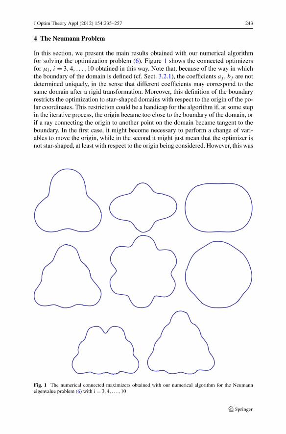
4 The Neumann Problem
In this section, we present the main results obtained with our numerical algorithmfor solving the optimization problem (6). Figure 1 shows the connected optimizersfor μi , i = 3,4, . . . ,10 obtained in this way. Note that, because of the way in whichthe boundary of the domain is defined (cf. Sect. 3.2.1), the coefficients aj , bj are notdetermined uniquely, in the sense that different coefficients may correspond to thesame domain after a rigid transformation. Moreover, this definition of the boundaryrestricts the optimization to star–shaped domains with respect to the origin of the po-lar coordinates. This restriction could be a handicap for the algorithm if, at some stepin the iterative process, the origin became too close to the boundary of the domain, orif a ray connecting the origin to another point on the domain became tangent to theboundary. In the first case, it might become necessary to perform a change of vari-ables to move the origin, while in the second it might just mean that the optimizer isnot star-shaped, at least with respect to the origin being considered. However, this was
Fig. 1 The numerical connected maximizers obtained with our numerical algorithm for the Neumanneigenvalue problem (6) with i = 3,4, . . . ,10
244 J Optim Theory Appl (2012) 154:235–257
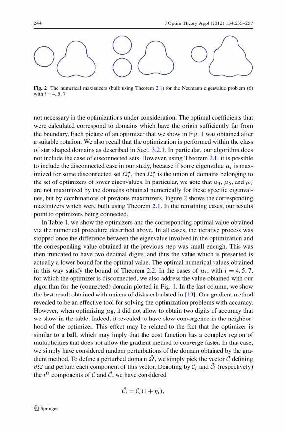
Fig. 2 The numerical maximizers (built using Theorem 2.1) for the Neumann eigenvalue problem (6)with i = 4, 5, 7
not necessary in the optimizations under consideration. The optimal coefficients thatwere calculated correspond to domains which have the origin sufficiently far fromthe boundary. Each picture of an optimizer that we show in Fig. 1 was obtained aftera suitable rotation. We also recall that the optimization is performed within the classof star shaped domains as described in Sect. 3.2.1. In particular, our algorithm doesnot include the case of disconnected sets. However, using Theorem 2.1, it is possibleto include the disconnected case in our study, because if some eigenvalue μi is max-imized for some disconnected set Ω�
i , then Ω�i is the union of domains belonging to
the set of optimizers of lower eigenvalues. In particular, we note that μ4, μ5, and μ7
are not maximized by the domains obtained numerically for these specific eigenval-ues, but by combinations of previous maximizers. Figure 2 shows the correspondingmaximizers which were built using Theorem 2.1. In the remaining cases, our resultspoint to optimizers being connected.
In Table 1, we show the optimizers and the corresponding optimal value obtainedvia the numerical procedure described above. In all cases, the iterative process wasstopped once the difference between the eigenvalue involved in the optimization andthe corresponding value obtained at the previous step was small enough. This wasthen truncated to have two decimal digits, and thus the value which is presented isactually a lower bound for the optimal value. The optimal numerical values obtainedin this way satisfy the bound of Theorem 2.2. In the cases of μi , with i = 4,5,7,for which the optimizer is disconnected, we also address the value obtained with ouralgorithm for the (connected) domain plotted in Fig. 1. In the last column, we showthe best result obtained with unions of disks calculated in [19]. Our gradient methodrevealed to be an effective tool for solving the optimization problems with accuracy.However, when optimizing μ8, it did not allow to obtain two digits of accuracy thatwe show in the table. Indeed, it revealed to have slow convergence in the neighbor-hood of the optimizer. This effect may be related to the fact that the optimizer issimilar to a ball, which may imply that the cost function has a complex region ofmultiplicities that does not allow the gradient method to converge faster. In that case,we simply have considered random perturbations of the domain obtained by the gra-dient method. To define a perturbed domain Ω , we simply pick the vector C defining∂Ω and perturb each component of this vector. Denoting by Ci and Ci (respectively)the ith components of C and C , we have considered
Ci = Ci (1 + ηi),
J Optim Theory Appl (2012) 154:235–257 245
Table 1 The Neumannmaximizers with the optimalvalues for μ�
iand the
corresponding multiplicity; thelast column shows the optimalvalue for unions of discs
where ηi is a random number generated in the interval [−0.05,0.05]. Then, if theeigenvalue of Ω is larger than the corresponding value of Ω , we define a new vectorC = C and repeat the process until an accuracy of two digits had been obtained.
5 The Dirichlet Problem
Now we present our results for the Dirichlet case. As stated in the Introduction, asimilar numerical study using a different method had already been performed byOudet in [4] for the first ten eigenvalues. With our method, we were able to ob-tain better results than those presented in that study. Moreover, we propose numeri-cal optimizers for more five eigenvalues. In Fig. 3, we plot these optimizers for λi ,i = 5,6, . . . ,15. Except for one case, there is agreement between the optimal shapesthat we obtained and those presented in [4]. The exception is related to the mini-mization of λ7, for which the optimal shape proposed by Oudet is disconnected andwas built using the Wolf–Keller theorem. On the other hand, we have obtained theconnected set which is plotted in Fig. 3 and has a smaller eigenvalue. This differencebetween Oudet’s results and ours may be related with the bound of Theorem 2.2. Wenote that while all our numerical optimal values satisfy that bound, Oudet’s resultsfor λ∗
6 and λ∗7 do not. In Table 2, we show the numerical values obtained here and
those obtained in [4]. In this study, we only aimed at an accuracy of two decimaldigits. The MFS with an adequate choice for the point sources is a highly accuratenumerical method, especially for smooth domains as those we deal with in this opti-mization procedure [22, 27]. We thus believe that the numerical approximations forthe eigenvalues of our numerical optimizers have at least two decimal digits of ac-curacy, which could be confirmed using the Moler–Payne theorem [22, 28]. All thevalues indicated were obtained rounding up our numerical values and are thus upperbounds for the optimal value.
We remark also that with some extra computational time the method employedcan easily provide more accuracy in the calculation of the optimal eigenvalue. Toillustrate this, we have considered the domain optimizing λ10. This has multiplicity 4
246 J Optim Theory Appl (2012) 154:235–257
Fig. 3 The optimizers for the Dirichlet eigenvalue problem (5) with i = 5,6, . . . ,15
and we should thus have
λ10(Ω∗
10
) = λ9(Ω∗
10
) = λ8(Ω∗
10
) = λ7(Ω∗
10
).
With our algorithm, we obtained a domain for which λ7 ≈ 142.7171281625934 andλ10 ≈ 142.7171281626059, the difference between the two values being 1.25 ×10⁻¹¹.
As in the Neumann case, the way in which the domains were defined, described inSect. 3.2.1, restricts the numerical optimization to star-shaped domains with respectto the origin. Again, this could be a limitation if any of the situations mentioned
J Optim Theory Appl (2012) 154:235–257 247
Table 2 Dirichlet minimizerswith the optimal values for λ∗
iand the correspondingmultiplicity
Fig. 4 The numerical optimizers for λ13 and λ15 and the corresponding center of mass
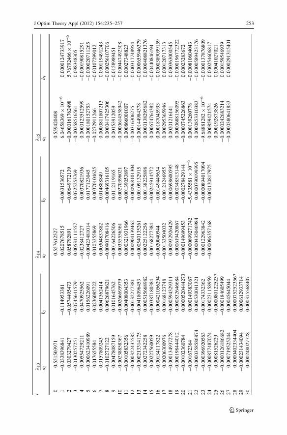
above occurred. However, and as in the Neumann case, the coefficients calculatedby our numerical algorithm correspond to domains having the origin sufficiently farfrom the boundary, and with no rays becoming tangent to it. To illustrate this fact, inFig. 4, we plot the numerical optimizers for λ13 and λ15. In both cases, we mark alsothe origin and the center of mass of the domain.
We also note that the optimizer for λ13 does not seem to have any kind of sym-metry. It would be natural to assume this to be an artifact of the algorithm, due to thefact that the location of the origin of our coordinate system is far from the center ofmass of the domain. However, this does not seem to be the case, as can be seen byperforming a change of variables to move the origin to the center of mass and thenrestart the optimization procedure. When we do this, we find that the results obtained
248 J Optim Theory Appl (2012) 154:235–257
do not differ in a significant way and, in particular, the numerical optimizer for λ13remains without any symmetries.
6 Symmetries, Multiplicities, and TRIANGULAR Domains
An analysis of the optimizers obtained suggests several remarks and directions for fu-ture study, both numerically and analytically. One first issue is related to symmetry.It is part of the folklore of this subject that optimizers should have some sort of sym-metry. Although this seems to be the case in most situations, we found one example,λ13, for which there seems to be no symmetry involved. Due to the high multiplicitiesinvolved and to the complexity of the optimization procedure we cannot, of course,ensure that there does not exist another domain—which does not necessarily have tobe close to this one—for which λ13 is lower than the one given here. We have consid-ered the optimization of λ13 among domains which are symmetric by reflection withrespect to some line. Instead of the expansion (12), we have considered
r(t) ≈ r(t) :=M∑
j=0
aj cos(j t) (17)
and then optimized the coefficients aj , j = 0, . . . ,M to minimize λ13|Ω|. Our sym-metric numerical optimizer is plotted in Fig. 5 together with the optimizer obtainedwithout symmetry constraint. For this symmetric domain, we obtained λ13 = 187.92which, due to the high accuracy of the MFS, we believe to be significantly larger than186.97 which was obtained without symmetry constraint.
This should be a matter for further study since, as mentioned in the Introduction,proving the existence of symmetries of optimizers is one of the important aspectsfrom a theoretical point of view.
In all other cases, both for the Dirichlet and Neumann problems, the examplesconsidered suggest the existence of either a reflection or Z3 symmetry (or both). Wenote that this can be checked in a more precise way than by just looking at the picture,as we will now illustrate. The picture for the optimizer of λ15 strongly suggests that
Fig. 5 Symmetric numerical minimizer of λ13 and the optimizer obtained without symmetry constraint
J Optim Theory Appl (2012) 154:235–257 249
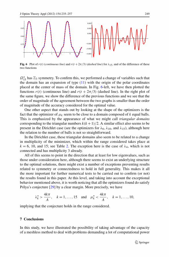
Fig. 6 Plot of r(t) (continuous line) and r(t + 2π/3) (dashed line) for λ15, and of the difference of thesetwo functions
Ω∗15 has Z3 symmetry. To confirm this, we performed a change of variables such that
the domain has an expansion of type (11) with the origin of the polar coordinatesplaced at the center of mass of the domain. In Fig. 6-left, we have then plotted thefunctions r(t) (continuous line) and r(t + 2π/3) (dashed line). In the right plot ofthe same figure, we show the difference of the previous functions and we see that theorder of magnitude of the agreement between the two graphs is smaller than the orderof magnitude of the accuracy considered for the optimal value.
One other aspect that stands out by looking at the shape of the optimizers is thefact that the optimizer of μk seem to be close to a domain composed of k equal balls.This is emphasized by the appearance of what we might call triangular domainscorresponding to the triangular numbers k(k +1)/2. A similar effect also seems to bepresent in the Dirichlet case (see the optimizers for λ6, λ10, and λ15), although herethe relation to the number of balls is not so straightforward.
In the Dirichlet case, these triangular domains also seem to be related to a changein multiplicity of the minimizer, which within the range considered takes place atk = 6, 10, and 15; see Table 2. The exception here is the case of λ4, which is notconnected and has multiplicity 3 already.
All of this seems to point in the direction that at least for low eigenvalues, such asthose under consideration here, although there seems to exist an underlying structureto the optimal solutions, there might exist a number of exceptions preventing resultsrelated to symmetry or connectedness to hold in full generality. This makes it allthe more important for further numerical tests to be carried out to confirm (or not)the results found in this paper. At this level, and taking into account the exceptionalbehavior mentioned above, it is worth noticing that all the optimizers found do satisfyPólya’s conjecture [29] by a clear margin. More precisely, we have
λ∗k >
4kπ
A, k = 1, . . . ,15 and μ∗
k <4kπ
A, k = 1, . . . ,10,
implying that the conjecture holds in the range considered.
7 Conclusions
In this study, we have illustrated the possibility of taking advantage of the capacityof a meshless method to deal with problems demanding a lot of computational power
250 J Optim Theory Appl (2012) 154:235–257
while keeping accuracy within required levels, by applying it to the optimization oflow Dirichlet and Neumann eigenvalues of the Laplace operator.
We have confirmed most of the results from a previous study of the Dirichlet caseby Oudet using different methods [4], and provided a domain with a better value inthe case of λ7. Besides this, we have determined the candidates for optimizers for fivemore eigenvalues up to λ15.
In the Neumann case, more challenging from a computational point of view, wedetermined numerical candidates for maximizers up to μ10.
The numerical coefficients defining the numerical Dirichlet and Neumann opti-mizers are provided in the Appendix.
The results obtained reveal a rich structure behind the optimizers pertaining tosymmetry, connectedness, and multiplicities. However, we also found some excep-tions which we believe to be of interest, such as the fact that it is likely that theoptimizer of the 13th Dirichlet eigenvalue will not have any kind of symmetry. As faras we are aware, it is the first example of this type which appears in the literature. Inview of these results, it would seem that although optimizers do possess an underly-ing structure, it might not be possible to establish general results due to the existenceof exceptions.
It is possible, of course, to do some variations around the cases considered here.Although we have considered mainly the case of star-shaped domains, the case of adisconnected domain composed of several star-shaped components was also includedby means of the Wolf–Keller theorem. However, we did not consider domains withholes, as these are not expected to yield better values than simply-connected domains.If desired, the MFS can also be applied in that case [30], and thus with the appropriatemodifications, this study could be extended to include multiply connected domains.
A more interesting problem is the extension of the methods in this paper to thethree-dimensional case. This is a much more challenging situation, which is cur-rently under research. We believe that the Method of Fundamental Solutions with anappropriate choice for the source-points, as in [31], will also allow for a solution ofthis optimization problem in reasonable computational time.
Acknowledgements P.R.S.A. was partially supported by FCT, Portugal, through the scholarshipSFRH/BPD/47595/2008 and the project PTDC/MAT/105475/2008 and by Fundação Calouste Gulbenkianthrough program Estímulo à Investigação 2009. Both authors were partially supported by FCT’s projectPTDC/MAT/101007/2008.
1. Antunes, P., Freitas, P.: New bounds for the principal Dirichlet eigenvalue of planar regions. Exp.Math. 15, 333–342 (2006)
2. Antunes, P., Freitas, P.: A numerical study of the spectral gap. J. Phys. A 5(055201) (2008) 19 pp.3. Henrot, A., Oudet, E.: Minimizing the second eigenvalue of the Laplace operator with Dirichlet
boundary conditions. Arch. Ration. Mech. Anal. 169, 73–87 (2003)4. Oudet, E.: Numerical minimization of eigenmodes of a membrane with respect to the domain. ESAIM
Control Optim. Calc. Var. 10, 315–330 (2004)5. Courant, R., Hilbert, D.: Methods of Mathematical Physics, vol. I. Interscience, New York (1953)6. Henrot, A.: Extremum Problems for Eigenvalues of Elliptic Operators. Frontiers in Mathematics.
Birkhäuser, Basel (2006)7. Faber, G.: Beweis, dass unter allen homogenen membranen von gleicher flüche und gleicher spannung
die kreisfürmige den tiefsten grundton gibt. Sitz. ber. bayer. Akad. Wiss., 169–172 (1923)8. Krahn, E.: Über eine von Rayleigh formulierte minimaleigenschaft des kreises. Math. Ann. 94, 97–
100 (1924)9. Pólya, G.: On the characteristic frequencies of a symmetric membrane. Math. Z. 63, 331–337 (1955)
10. Krahn, E.: Über Minimaleigenshaften der Kugel in drei und mehr Dimensionen. Acta Comm. Univ.Dorpat. A9, 1–44 (1926)
J Optim Theory Appl (2012) 154:235–257 257
11. Kornhauser, E.T., Stakgold, I.: A variational theorem for ∇2u + λu = 0 and its applications. J. Math.Phys. 31, 45–54 (1952)
12. Szegö, G.: Inequalities for certain eigenvalues of a membrane of given area. Arch. Ration. Mech.Anal. 3, 343–356 (1954)
13. Weinberger, H.F.: An isoperimetric inequality for the N -dimensional free membrane problem. Arch.Ration. Mech. Anal. 5, 633–636 (1956)
14. Girouard, A., Nadirashvili, N., Polterovich, I.: Maximization of the second positive Neumann eigen-value for planar domains. J. Differ. Geom. 83(3), 637–662 (2009)
15. Bucur, D., Henrot, A.: Minimization of the third eigenvalue of the Dirichlet Laplacian. Proc. R. Soc.Lond. 456, 985–996 (2000)
16. Wolf, S.A., Keller, J.B.: Range of the first two eigenvalues of the Laplacian. Proc. R. Soc. Lond. Ser.A, Math. Phys. Sci. 447, 397–412 (1994)
17. Buttazzo, G., Dal Maso, G.: An existence result for a class of shape optimization problems. Arch.Ration. Mech. Anal. 122, 183–195 (1993)
18. Cox, S.J.: Extremal eigenvalue problems for starlike planar domains. J. Differ. Equ. 120(1), 174–197(1995)
19. Poliquin, G., Roy-Fortin, G.: Wolf-Keller theorem for Neumann eigenvalues. Ann. Sci. Math. Québec(to appear)
20. Colbois, B., El Soufi, A.: Extremal eigenvalues of the Laplacian on Euclidean domains and Rieman-nian manifolds (preprint)
21. Bogomolny, A.: Fundamental solutions method for elliptic boundary value problems. SIAM J. Numer.Anal. 22(4), 644–669 (1985)
22. Alves, C.J.S., Antunes, P.R.S.: The method of fundamental solutions applied to the calculation ofeigenfrequencies and eigenmodes of 2D simply connected shapes. Comput. Mater. Continua 2(4),251–266 (2005)
23. Goldberg, D.: Genetic Algorithms. Addison Wesley, Reading (1988)24. Nocedal, J., Wright, S.J.: Numerical Optimization. Springer, Berlin (1999)25. Snyman, J.A.: Practical Mathematical Optimization: An Introduction to Basic Optimization Theory
and Classical and New Gradient-Based Algorithms. Springer, Berlin (2005)26. Sokolowski, J., Zolesio, J.P.: Introduction to Shape Optimization: Shape Sensitivity Analysis.
Springer Series in Computational Mathematics, vol. 10. Springer, Berlin (1992)27. Barnett, A.H., Betcke, T.: Stability and convergence of the method of fundamental solutions for
Helmholtz problems on analytic domains. J. Comput. Phys. 227, 7003–7026 (2008)28. Moler, C.B., Payne, L.E.: Bounds for eigenvalues and eigenfunctions of symmetric operators. SIAM
J. Numer. Anal. 5, 64–70 (1968)29. Pólya, G.: On the eigenvalues of vibrating membranes. Proc. Lond. Math. Soc. 11, 419–433 (1961)30. Chen, J.T., Chen, I.L., Lee, Y.T.: Eigensolutions of multiply connected membranes using the method
of fundamental solutions. Eng. Anal. Bound. Elem. 29, 166–174 (2005)31. Antunes, P.R.S.: Numerical calculation of eigensolutions of 3D shapes using the method of funda-


![Isoperimetric Inequalities for Eigenvalues of the rbenguri/105.pdforthonormal basis of real eigenfunctions corresponding to the Dirichlet eigenvalues ... we refer to the book by Chavel [44] (pp. 86–94) and references therein.](https://static.documents.pub/doc/80x56/5af3b09c7f8b9a8c30917cc4/isoperimetric-inequalities-for-eigenvalues-of-the-rbenguri105pdforthonormal-basis.jpg)


