Numerical Optimization Algorithms

1. Overview2. Calculus of Variations3. Linearized Supersonic Flow4. Steepest Descent5. Smoothed Steepest Descent

Numerical Optimization AlgorithmsOverview 1

Two Main Categories of Optimization Algorithms

Gradient Based Non-Gradient Based

Numerical Optimization AlgorithmsOverview 2

• Only objective function evaluations are used to find optimum point. Gradient and Hessian of the objective function are not needed.

• May be able to find global minimum BUT requires a large number of design cycles.

• Non-gradient based family of methods: genetic algorithms, grid searchers, stochastic, nonlinear simplex, etc.

• In the case of Genetic Algorithms: Evaluations of the objective function of an initial set of solutions starts the design process. Initial set is typically very LARGE.

• Able to handle integer variables such as number of vertical tails, number of engines and other integer parameters.

• Able to seek the optimum point for objective functions that do not have smooth first or second derivatives.

Non-Gradient Based

Numerical Optimization AlgorithmsOverview 3

• Requires existence of continuous first derivatives of the objective function and possibly higher derivatives.

• Generally requires a much smaller number of design cycles to converge to an optimum compared to non-gradient based methods.

• However, only convergence to a local minimum is guaranteed.

• Simple gradient-based methods only require the gradient of the objective function but usually requires N2 iterations or more where N is the number of design variables.

• Methods that use the Hessian (Quasi-Newton) generally only require N iterations.

Gradient Based

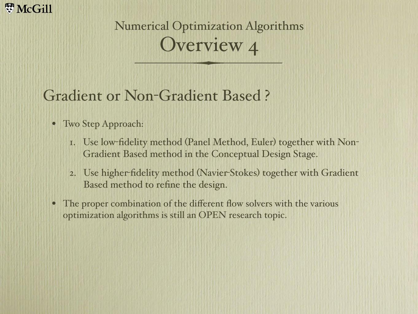
Numerical Optimization AlgorithmsOverview 4

• Two Step Approach:

1. Use low-fidelity method (Panel Method, Euler) together with Non-Gradient Based method in the Conceptual Design Stage.

2. Use higher-fidelity method (Navier-Stokes) together with Gradient Based method to refine the design.

• The proper combination of the different flow solvers with the various optimization algorithms is still an OPEN research topic.

Gradient or Non-Gradient Based ?

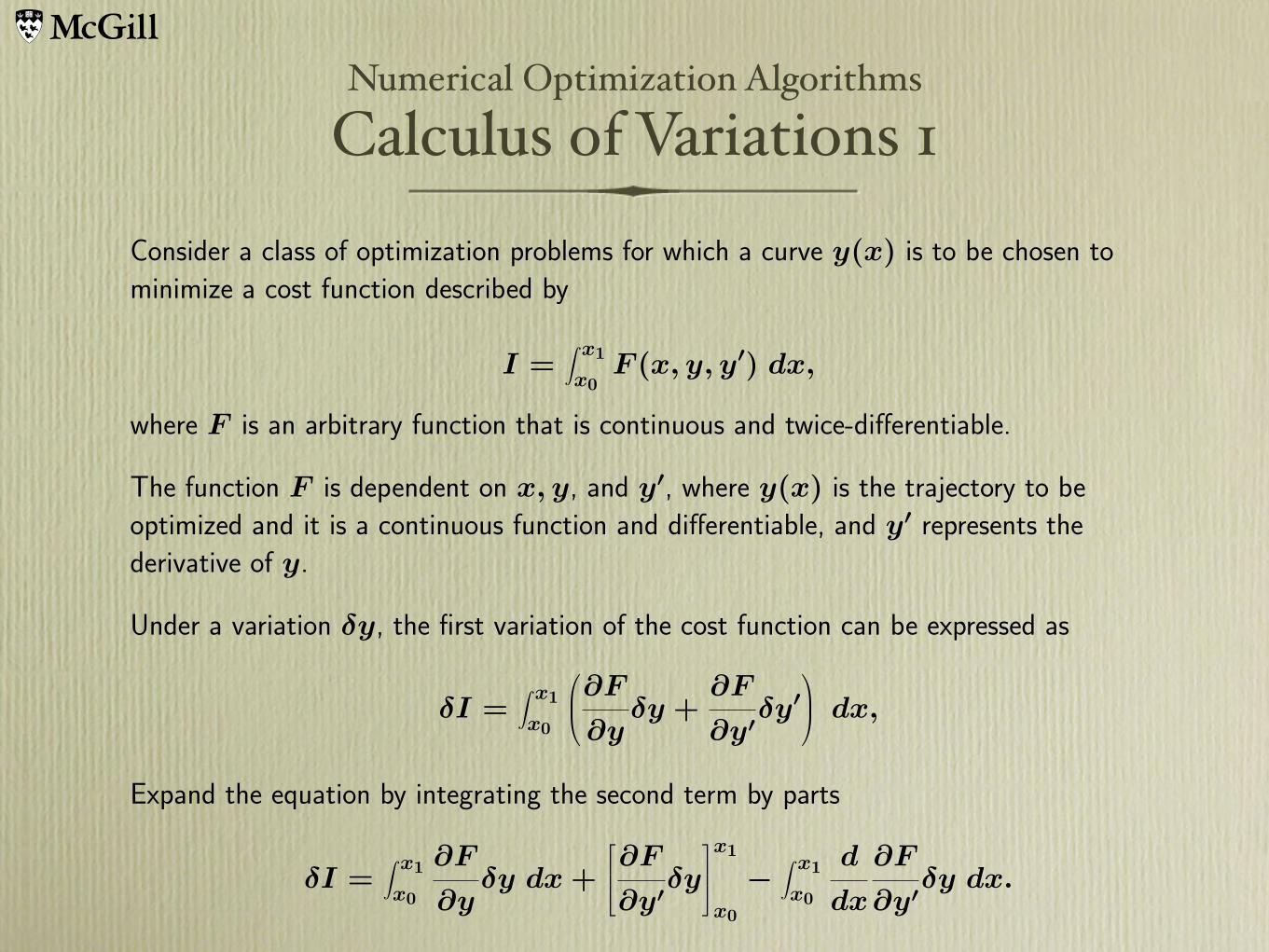
Numerical Optimization AlgorithmsCalculus of Variations 1

Consider a class of optimization problems for which a curve y(x) is to be chosen tominimize a cost function described by

I =∫ x1

x0F (x, y, y′) dx,

where F is an arbitrary function that is continuous and twice-differentiable.

The function F is dependent on x, y, and y′, where y(x) is the trajectory to beoptimized and it is a continuous function and differentiable, and y′ represents thederivative of y.

Under a variation δy, the first variation of the cost function can be expressed as

δI =∫ x1

x0

∂F

∂yδy +

∂F

∂y′δy′ dx,

Expand the equation by integrating the second term by parts

δI =∫ x1

x0

∂F

∂yδy dx +

∂F

∂y′δy

x1

x0

− ∫ x1

x0

d

dx

∂F

∂y′δy dx.

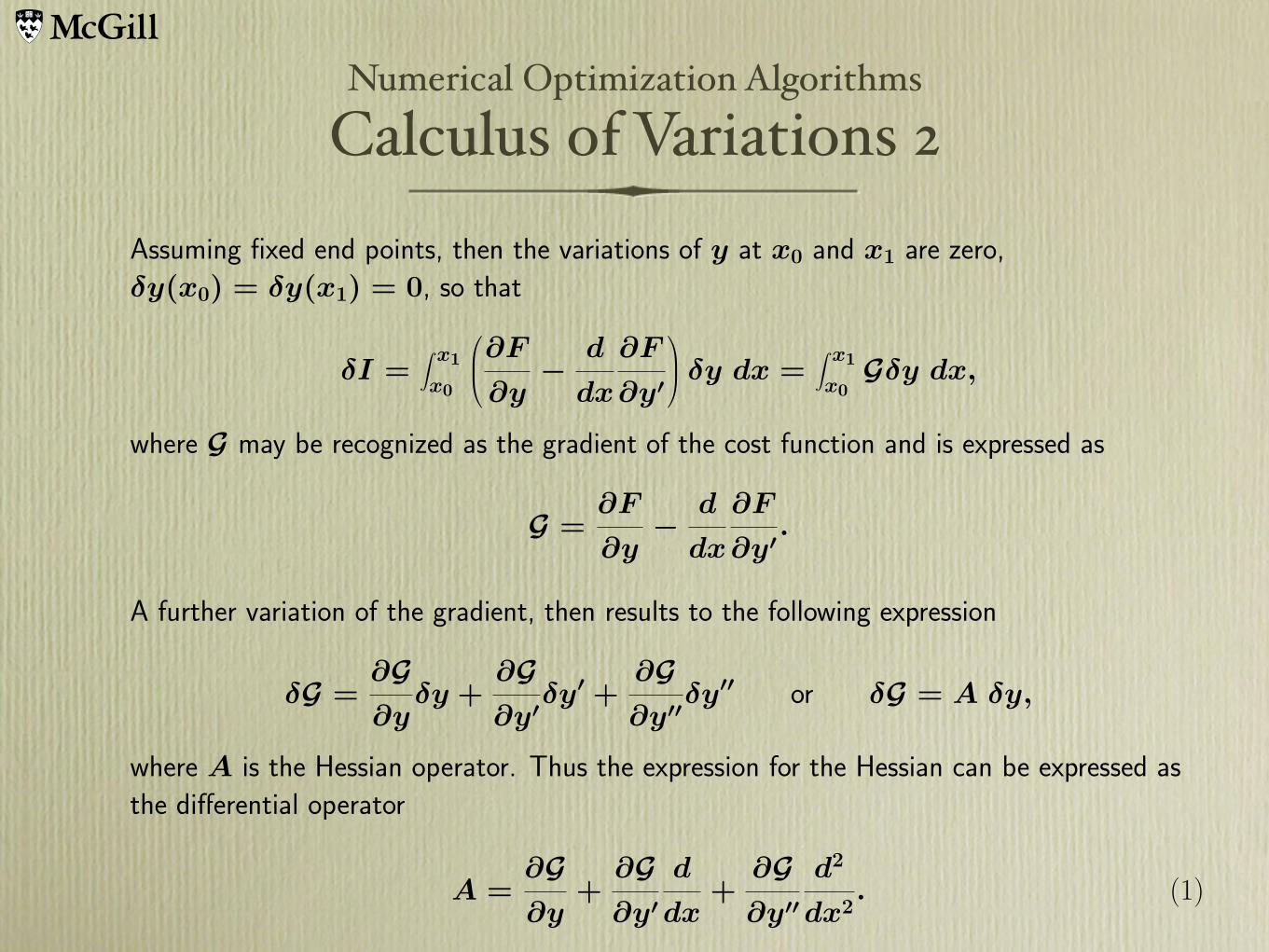
Numerical Optimization AlgorithmsCalculus of Variations 2

Assuming fixed end points, then the variations of y at x0 and x1 are zero,δy(x0) = δy(x1) = 0, so that

δI =∫ x1

x0

∂F

∂y− d

dx

∂F

∂y′

δy dx =∫ x1

x0Gδy dx,

where G may be recognized as the gradient of the cost function and is expressed as

G =∂F

∂y− d

dx

∂F

∂y′ .

A further variation of the gradient, then results to the following expression

δG =∂G∂y

δy +∂G∂y′δy′ +

∂G∂y′′δy′′ or δG = A δy,

where A is the Hessian operator. Thus the expression for the Hessian can be expressed asthe differential operator

A =∂G∂y

+∂G∂y′

d

dx+

∂G∂y′′

d2

dx2. (1)

Numerical Optimization AlgorithmsLinearized Supersonic Flow 1

In this example, we explore this concept by deriving the gradient and Hessian operator forlinearized supersonic flow.

Consider a linearized supersonic flow over a profile with a height y(x), where y iscontinuous and twice-differentiable. The surface pressure can be defined as

p − p∞ = − ρq2√M2∞ − 1

dy

dx,

where ρq2√M2∞−1

is a constant and p∞ is the freestream pressure. Next consider an inverse

problem with cost function

I =1

2

∫B

(p − pt)2 dx,

where pt is the target surface pressure. The variation of the equation for the surfacepressure and cost function under a profile variation δy is

δp = − ρq2√M2∞ − 1

d

dxδy and δI =

∫B

(p − pt) δp dx.

Numerical Optimization AlgorithmsLinearized Supersonic Flow 2

Substitute the variation of the pressure into the equation for the variation of the costfunction and integrate by parts to obtain

δI = − ∫B(p − pt)

ρq2√M2∞ − 1

d

dxδy dx

=∫B

ρq2√M2∞ − 1

d

dx(p − pt)δy dx.

The gradient can then be defined as

g =ρq2√

M2∞ − 1

d

dx(p − pt).

Numerical Optimization AlgorithmsLinearized Supersonic Flow 3

To form the Hessian, take a variation of the gradient and substitute the expression for δp

δg =ρq2√

M2∞ − 1

d

dxδp = − ρ2q4

M2∞ − 1

d2

dx2δy.

Thus the Hessian for the inverse design of the linearized supersonic flow problem can beexpressed as the differential operator

A = − ρ2q4

M2∞ − 1

d2

dx2. (2)

Numerical Optimization AlgorithmsBrachistochrone 1

Brachistochorne Problem: Find the minimum time taken by a particle traversing a pathy(x) connecting initial and final points (xo, yo) and x1, y1), subject only to the force ofgravity. The total time is given by

T =∫ x1

xo

ds

v

where the velocity of a particel starting from rest and falling under the influence of gravityis

v =√

2gy

and

ds2 = dx2 + dy2 ds

dx

2

= 1 +

dy

dx

2

ds =√1 + y′2dx

Numerical Optimization AlgorithmsBrachistochrone 2

Substitution for v and ds, yields

T =∫ x1

xo

√1 + y′2√

2gydx =

1

2g

∫ x1

xo

√√√√√√1 + y′2

ydx =

I

2g

Therefore,

I =∫ x1

xo

√√√√√√1 + y′2

ydx =

∫ x1

xoF (y, y′)dx

From Calculus of Variations,

G = Fy − d

dxFy′ =

∂F

∂y− d

dx

∂F

∂y′

Compute the partial derivatives of F with respect to y and y′ and substitute into thegradient formula produces

G = −√

1 + y′2

2y32

− d

dx

y′√y(1 + y′2)

Numerical Optimization AlgorithmsBrachistochrone 3

The expression for the gradient can then be simplified to

G = −1 + y′2 + 2yy′′

2(y(1 + y′2))32

Since F does not depend on x,

G = Fy − d

dxFy′ = Fy − Fy′x − Fy′yy

′ − Fy′y′y′′

y′G = Fyy′ − Fy′yy

′2 − Fy′y′y′′y′ =d

dx(F − y′Fy′)

On an optimal path, G = 0, so

y′G =d

dx(F − y′Fy′) = 0

orF − y′Fy′ = const

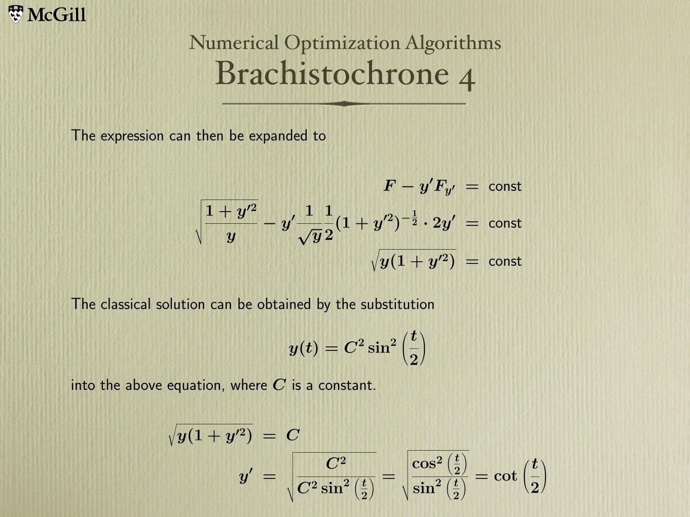
Numerical Optimization AlgorithmsBrachistochrone 4

The expression can then be expanded to

F − y′Fy′ = const√√√√√√1 + y′2

y− y′ 1√

y

1

2(1 + y′2)−1

2 · 2y′ = const

√y(1 + y′2) = const

The classical solution can be obtained by the substitution

y(t) = C2 sin2 t

2

into the above equation, where C is a constant.

√y(1 + y′2) = C

y′ =

√√√√√√√ C2

C2 sin2(

t2

) =

√√√√√√√cos2(

t2

)sin2

(t2

) = cot t

2

Numerical Optimization AlgorithmsBrachistochrone 5

Finally, the optimal path can be derived by substituting y′ in the previous equation withdydx

to yield

dy

dx= cot

t

2

x =

∫ y

cot(

t2

) =∫

tan t

2

dy

dtdt =

∫C2 sin2

t

2

dt

x(t) =1

2C2(t − sin t)

Numerical Optimization AlgorithmsBrachistochrone 6: Continuous Grad

Let the trajectory be represented by the discrete values

yj = y(xj) at xj = j∆x

where ∆x is the mesh interval, j is defined as 0 ≤ j ≤ N + 1 and N is the number ofdesign variables which are also the number of mesh points.

From the gradient obtained through calculus of variations, the continuous gradient can becomputed as

Gj = −1 + y′2j + 2yjy′′

j

2(yj(1 + y′2j ))

32

where y′j and y′′

j can be evaluated at the discrete points using second-order finitedifference approximation

y′j =

yj+1 − yj−1

2∆x,and y′′

j =yj+1 − 2yj + yj−1

∆x2

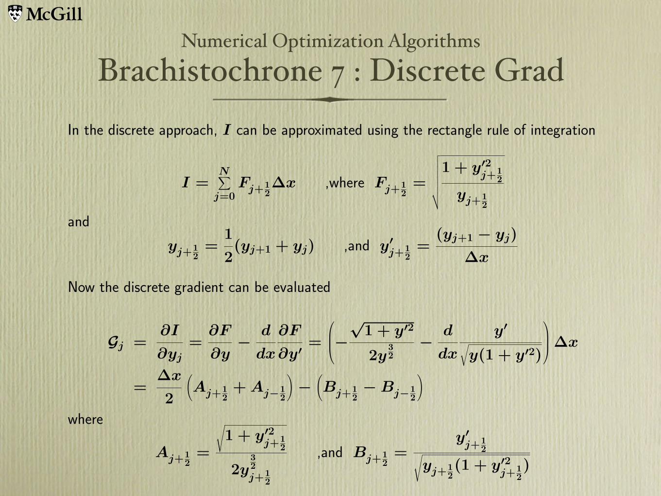
Numerical Optimization AlgorithmsBrachistochrone 7 : Discrete Grad

In the discrete approach, I can be approximated using the rectangle rule of integration

I =N∑

j=0Fj+1

2∆x ,where Fj+1

2=

√√√√√√√√1 + y′2

j+12

yj+12

and

yj+12

=1

2(yj+1 + yj) ,and y′

j+12

=(yj+1 − yj)

∆x

Now the discrete gradient can be evaluated

Gj =∂I

∂yj=

∂F

∂y− d

dx

∂F

∂y′ =

−√

1 + y′2

2y32

− d

dx

y′√y(1 + y′2)

∆x

=∆x

2

(Aj+1

2+ Aj−1

2

)−

(Bj+1

2− Bj−1

2

)

where

Aj+12

=

√1 + y′2

j+12

2y32j+1

2

,and Bj+12

=y′

j+12√

yj+12(1 + y′2

j+12)

Numerical Optimization AlgorithmsSteepest Descent 1

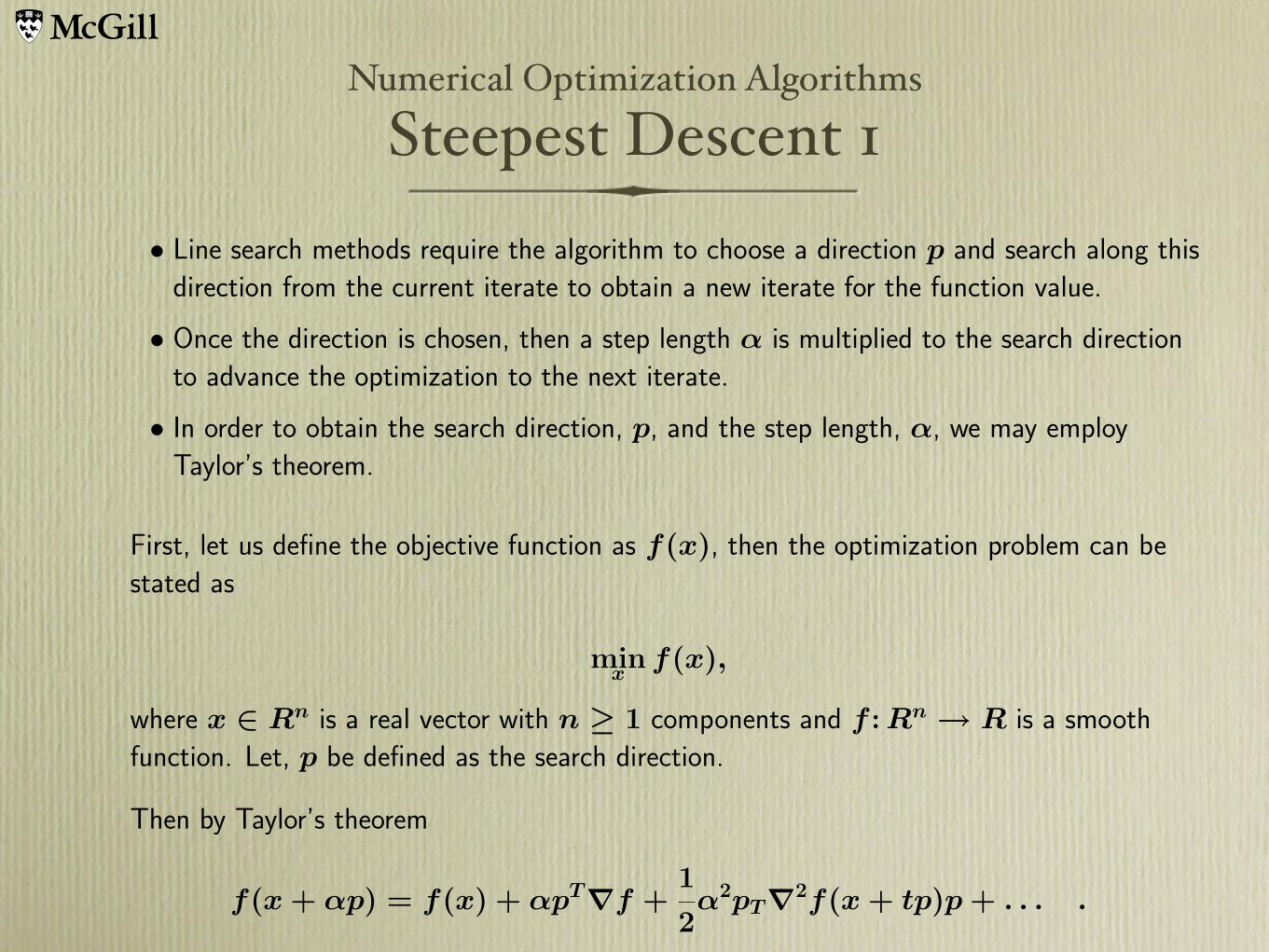
• Line search methods require the algorithm to choose a direction p and search along thisdirection from the current iterate to obtain a new iterate for the function value.

• Once the direction is chosen, then a step length α is multiplied to the search directionto advance the optimization to the next iterate.

• In order to obtain the search direction, p, and the step length, α, we may employTaylor’s theorem.

First, let us define the objective function as f(x), then the optimization problem can bestated as

minx

f(x),

where x ∈ Rn is a real vector with n ≥ 1 components and f : Rn → R is a smoothfunction. Let, p be defined as the search direction.

Then by Taylor’s theorem

f(x + αp) = f(x) + αpT∇f +1

2α2pT∇2f(x + tp)p + . . . .

Numerical Optimization AlgorithmsSteepest Descent 2

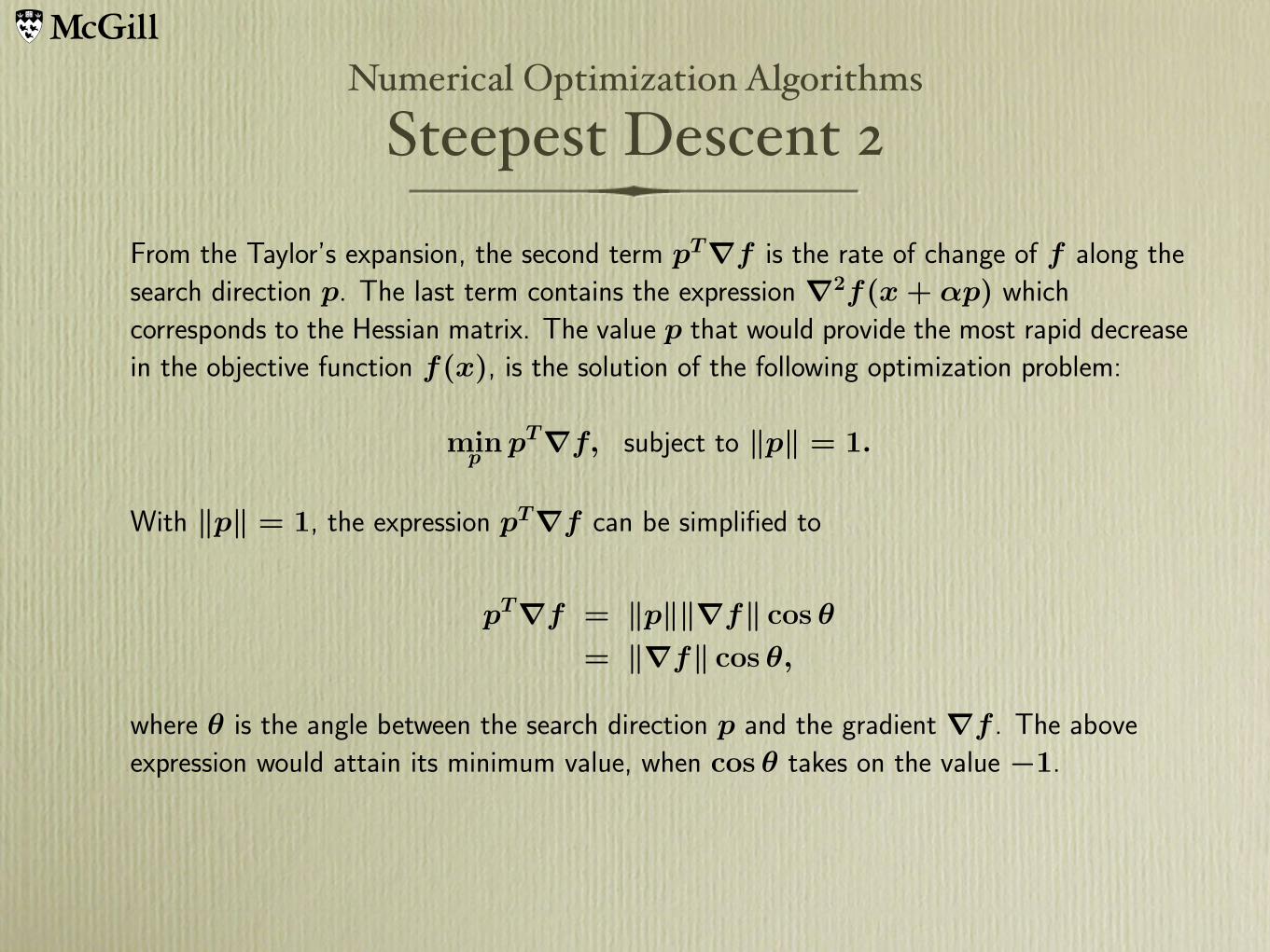
From the Taylor’s expansion, the second term pT∇f is the rate of change of f along thesearch direction p. The last term contains the expression ∇2f(x + αp) whichcorresponds to the Hessian matrix. The value p that would provide the most rapid decreasein the objective function f(x), is the solution of the following optimization problem:

minp

pT∇f, subject to ‖p‖ = 1.

With ‖p‖ = 1, the expression pT∇f can be simplified to

pT∇f = ‖p‖‖∇f‖ cos θ

= ‖∇f‖ cos θ,

where θ is the angle between the search direction p and the gradient ∇f . The aboveexpression would attain its minimum value, when cos θ takes on the value −1.

Numerical Optimization AlgorithmsSteepest Descent 3

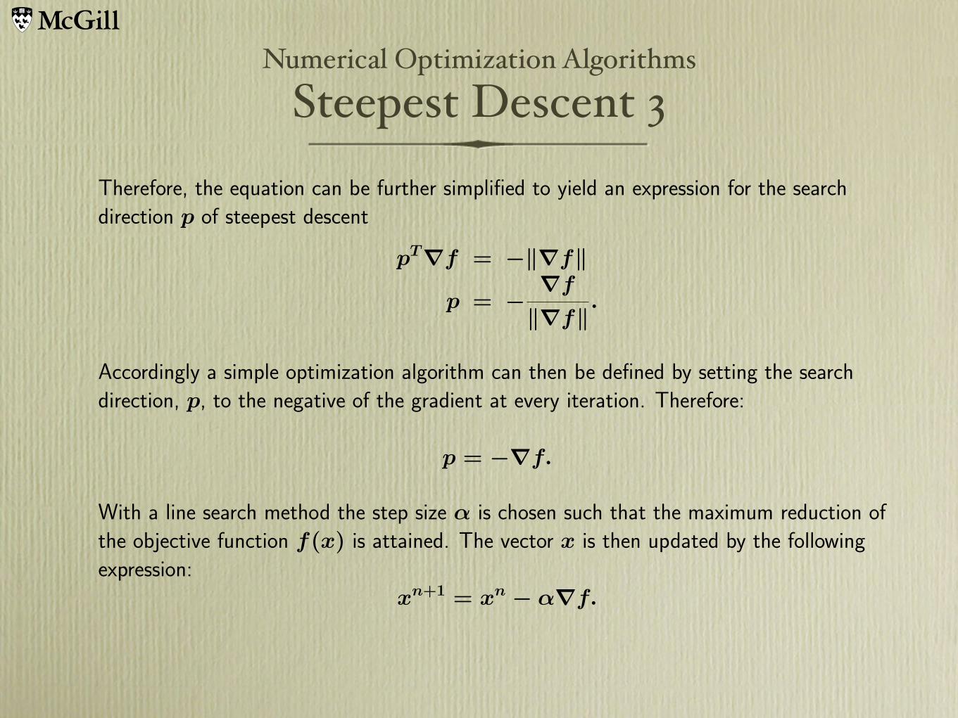
Therefore, the equation can be further simplified to yield an expression for the searchdirection p of steepest descent

pT∇f = −‖∇f‖p = − ∇f

‖∇f‖.

Accordingly a simple optimization algorithm can then be defined by setting the searchdirection, p, to the negative of the gradient at every iteration. Therefore:

p = −∇f.

With a line search method the step size α is chosen such that the maximum reduction ofthe objective function f(x) is attained. The vector x is then updated by the followingexpression:

xn+1 = xn − α∇f.

Numerical Optimization AlgorithmsSteepest Descent 4

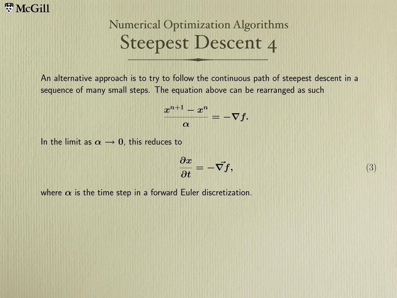
An alternative approach is to try to follow the continuous path of steepest descent in asequence of many small steps. The equation above can be rearranged as such

xn+1 − xn

α= −∇f.

In the limit as α → 0, this reduces to

∂x

∂t= − #∇f, (3)

where α is the time step in a forward Euler discretization.

Numerical Optimization AlgorithmsSmoothed Steepest Descent 1

Let x represent the design variable, and ∇f the gradient. Instead of making the step

δx = αp = −α∇f,

we replace the gradient ∇f by a smoothed value ∇f . To apply smoothing in the xdirection, the smoothed gradient ∇f may be calculated from a discrete approximation to

∇f − ∂

∂xε

∂

∂x∇f = ∇f, (4)

where ε is the smoothing parameter.

Then the first order change in the cost function is

δf = − ∫∫ ∇fδxdx

= −α∫∫ ∇f − ∂

∂xε

∂

∂x∇f

∇fdx

= −α∫∫ ∇f

2dx + α

∫∫ ∂

∂xε

∂

∂x∇f

∇fdx.

Numerical Optimization AlgorithmsSmoothed Steepest Descent 2

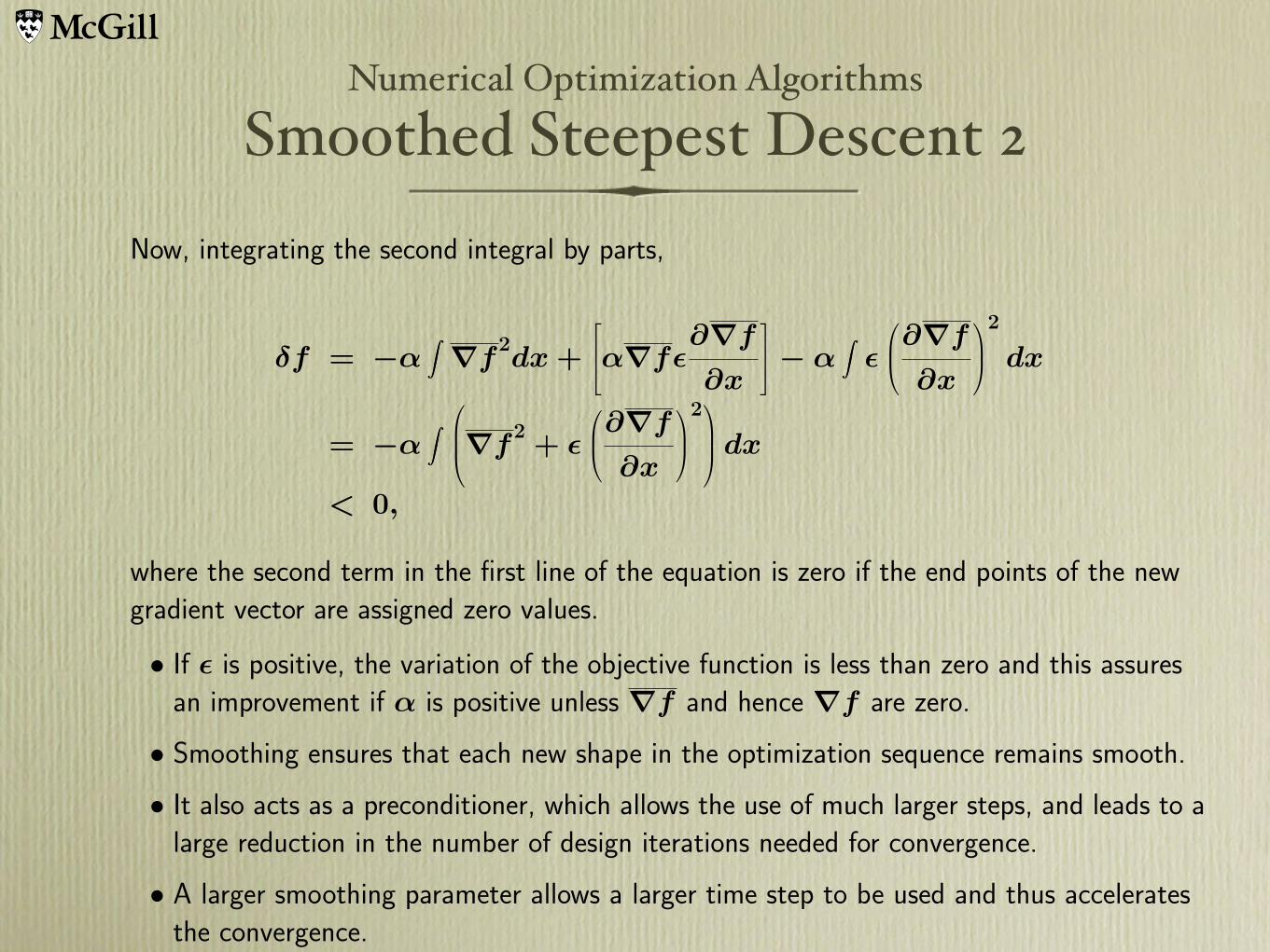
Now, integrating the second integral by parts,

δf = −α∫∫ ∇f

2dx +

α∇fε∂∇f

∂x

− α∫∫

ε

∂∇f

∂x

2

dx

= −α∫∫ ∇f

2+ ε

∂∇f

∂x

2 dx

< 0,

where the second term in the first line of the equation is zero if the end points of the newgradient vector are assigned zero values.

• If ε is positive, the variation of the objective function is less than zero and this assuresan improvement if α is positive unless ∇f and hence ∇f are zero.

• Smoothing ensures that each new shape in the optimization sequence remains smooth.

• It also acts as a preconditioner, which allows the use of much larger steps, and leads to alarge reduction in the number of design iterations needed for convergence.

• A larger smoothing parameter allows a larger time step to be used and thus acceleratesthe convergence.

Numerical Optimization AlgorithmsSmoothed Steepest Descent 3

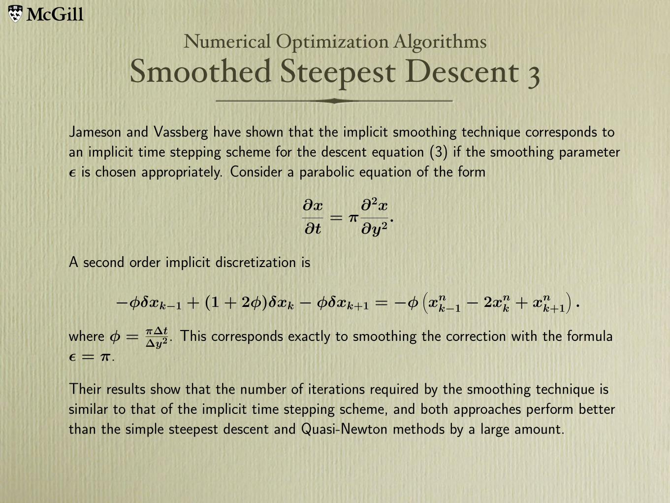
Jameson and Vassberg have shown that the implicit smoothing technique corresponds toan implicit time stepping scheme for the descent equation (3) if the smoothing parameterε is chosen appropriately. Consider a parabolic equation of the form

∂x

∂t= π

∂2x

∂y2.

A second order implicit discretization is

−φδxk−1 + (1 + 2φ)δxk − φδxk+1 = −φ(xn

k−1 − 2xnk + xn

k+1

).

where φ = π∆t∆y2 . This corresponds exactly to smoothing the correction with the formula

ε = π.

Their results show that the number of iterations required by the smoothing technique issimilar to that of the implicit time stepping scheme, and both approaches perform betterthan the simple steepest descent and Quasi-Newton methods by a large amount.

Numerical Optimization AlgorithmsSmoothed Steepest Descent 4

For some problems, such as the calculus of variations, the implicit smoothing techniquecan be used to implement the Newton method. In a Newton method, the gradient isdriven to zero based on the linearization

g(y + δy) = g(y) + Aδy,

where A is the Hessian. In the case of the calculus of variations a Newton step can beachieved by solving

Aδy =

∂G∂y

+∂G∂y′

d

dx+

∂G∂y′′

d2

dx2

δy = −g,

since the Hessian can be represented by the differential operator. Thus the correct choiceof smoothing from equation (4) approximates the Newton step, resulting in quadraticconvergence, independent of the number of mesh intervals.