Numerical relativity in spherical polar coordinates:

Calculations with the BSSN formulation

Pedro Montero

Max-Planck Institute for Astrophysics Garching (Germany)

Kyoto, 27/05/13

T.Baumgarte, I. Cordero-Carrion and E. Mueller

[ Phys. Rev. D 87, 044026 (2013)]

2

Introduction:motivationspherical polar coordinates and numerical relativitycovariant BSSN formulation treatment of singular terms

Partially implicit Runge-Kutta method (PIRK)Numerical implementation

Numerical examples:Weak gravitational wavesRotating relativistic starsSchwarzschild black hole

Evolution of the GR hydrodynamic equationsConclusions

Outline

3

Introduction Key ingredients for successful numerical relativity simulations:

Suitable formulation of Einstein equations: ● BSSN● Z4● Generalized Harmonic● Fully constraint formalism

Adequate gauge conditions for long-term stable evolutions● e.g. 1+log & gamma-freezing “family” conditions

Black hole treatment:

● excision● puncture technique

Numerical treatment:● finite differencing● spectral methods ● adaptive mesh refinement...

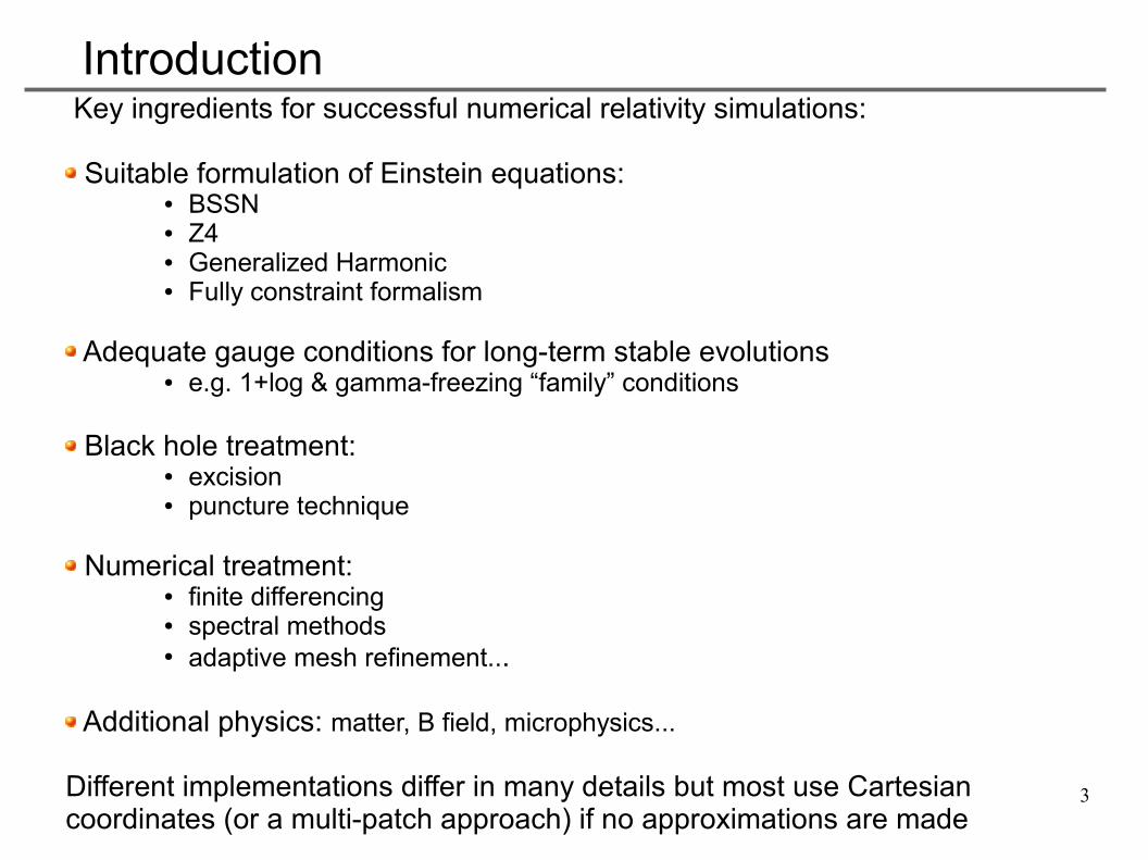
Additional physics: matter, B field, microphysics...

Different implementations differ in many details but most use Cartesian coordinates (or a multi-patch approach) if no approximations are made

4

Cartesian coordinates have many desirable properties

But for many astrophysical problems spherical polar coordinates seem better suited:

● Supernovae● Gravitational collapse● Accretion disks around BH

Implementing a numerical relativitycode in spherical polar coordinates possess several challenges

In particular, if we want to use a formulationlike BSSN some issues are:

Covariant BSSN formulationSingular terms in the equations

Introduction

5

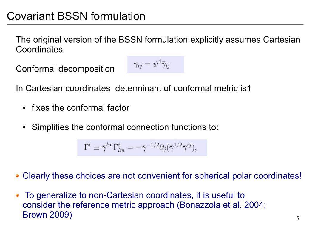
The original version of the BSSN formulation explicitly assumes Cartesian Coordinates

Conformal decomposition

In Cartesian coordinates determinant of conformal metric is1

● fixes the conformal factor

● Simplifies the conformal connection functions to:

Clearly these choices are not convenient for spherical polar coordinates!

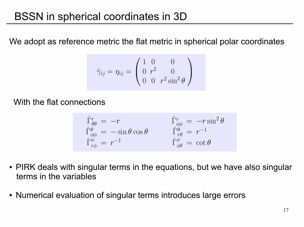
To generalize to non-Cartesian coordinates, it is useful to consider the reference metric approach (Bonazzola et al. 2004;Brown 2009)

Covariant BSSN formulation

6

It is useful to introduce the reference connections associated with the flat metric and then define the difference

These transform as tensor

For the flat reference metric in Cartesian coordinates

In spherical polar coordinates, flat reference connections absorb the singular terms (known analytically)

These are computed from

Reference metric

ij

jki

7

Then define

Conformal connections functions

Which transforms as a tensor, and then the conformal connectionfunctions are

Then the Ricci tensor associated to the conformal metric can be written as

Note that when is chosen to be the flat metric Rij=0ij

8

Brown (2009)

Covariant BSSN formulation

Now we have the covariant form of the equations and next, we have to deal with our choice of (curvilinear) coordinates

9

Spherical polar coordinates: singular terms in the equations

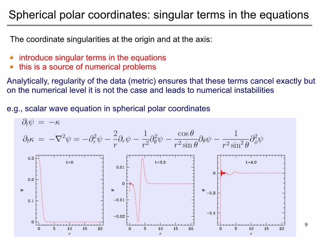
The coordinate singularities at the origin and at the axis:

introduce singular terms in the equations this is a source of numerical problems

Analytically, regularity of the data (metric) ensures that these terms cancel exactly but on the numerical level it is not the case and leads to numerical instabilities

e.g., scalar wave equation in spherical polar coordinates

10

0) Avoid them: Cartesian coordinates+Cartoon method

1) Specific gauge choice (i.e. polar/aereal gauges) [Bardeen & Piran 1983; Choptuik 1991]

Restricts the gauge freedom

We know that this is a crucial ingredient in successful numerical relativity simulations

2) Regularization method by imposing appropiate parity regularity conditions and local flatness [Alcubierre et al. 2005, Ruiz et al. 2007, Alcubierre et al. 2011]

Need to introduce auxiliary variables and new evolution equationsQuite cumbersome to implementProbably not trivial to investigate BH formation No scheme has been implemented without any symmetry assumptions

Handling coordinate singularities in Einstein equations

11

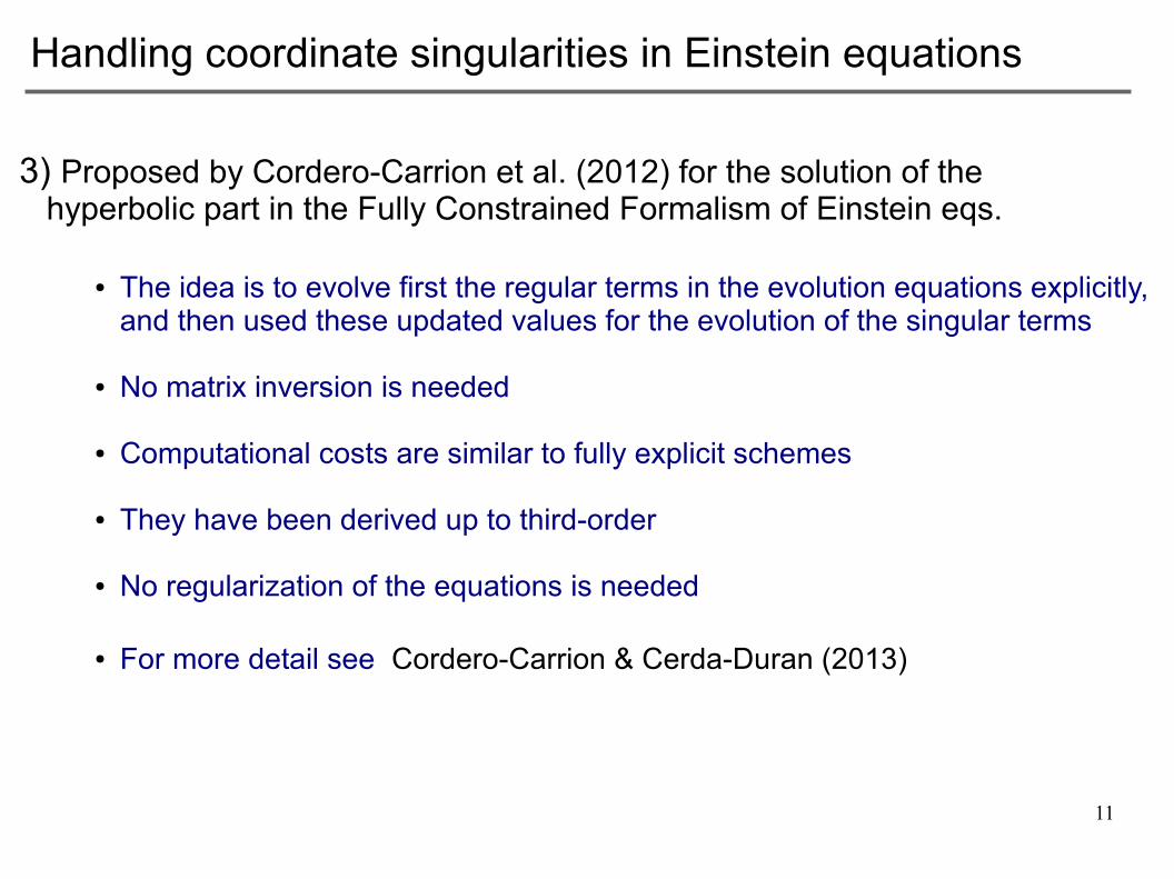
3) Proposed by Cordero-Carrion et al. (2012) for the solution of the hyperbolic part in the Fully Constrained Formalism of Einstein eqs.

● The idea is to evolve first the regular terms in the evolution equations explicitly, and then used these updated values for the evolution of the singular terms

● No matrix inversion is needed

● Computational costs are similar to fully explicit schemes

● They have been derived up to third-order

● No regularization of the equations is needed

● For more detail see Cordero-Carrion & Cerda-Duran (2013)

Handling coordinate singularities in Einstein equations

12

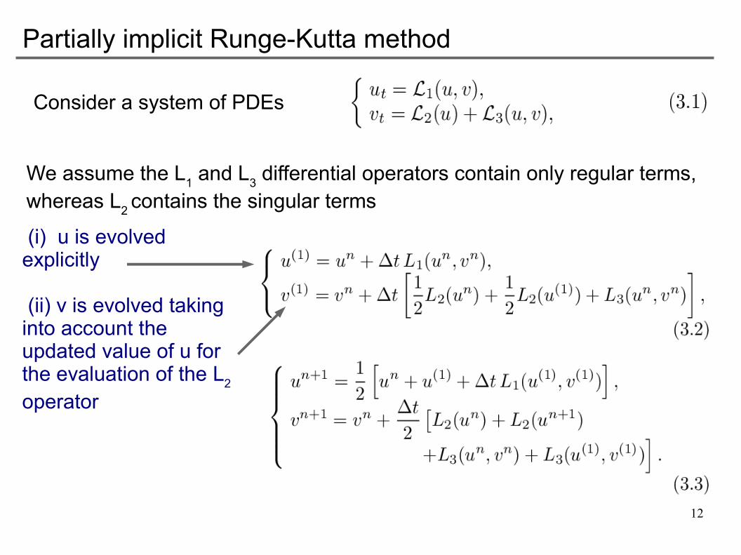
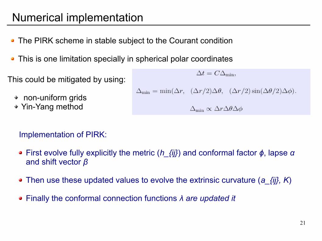
Partially implicit Runge-Kutta method

(i) u is evolved explicitly

(ii) v is evolved taking into account the updated value of u for the evaluation of the L2 operator

Consider a system of PDEs

We assume the L1 and L3 differential operators contain only regular terms, whereas L2 contains the singular terms

13

● PM & Cordero-Carrion (PRD,2012) applied successfully the PIRK method to the BSSN+GRHydro eqs. in spherical coordinates under the only assumption of spherical symmetry

Spatial line element:

Evolution equations

Application of PIRK to BSSN equations in 1D

14

Numerical examples 1D: pure gauge dynamics

- Initial data:

15

Numerical examples 1D: spherical relativistic stars

Stable TOV initial data Gravitational collapse of marginally stable TOV

16

Advantages:

Keep the gauge freedom (use 1+log, Gamma-driver)No need for a regularization scheme at origin or axisSimple implementation

Numerical examples 1D: spherical relativistic stars

17

BSSN in spherical coordinates in 3D

We adopt as reference metric the flat metric in spherical polar coordinates

With the flat connections

● PIRK deals with singular terms in the equations, but we have also singular terms in the variables

● Numerical evaluation of singular terms introduces large errors

18

Write the conformal metric

We scale out singular terms from all tensorial quantities

Singular terms in variables

1) Choose an orthonormal base so that the r, sinθ are absorbed into the unite vector

2) Coordinate base approach: scale out the appropriate powers of r and sinθ

and we write all equations in terms of the rescaled variables

19

We compute derivatives of the spatial metric as follows:

Which is written in terms of hi j

In the Ricci tensor,

We compute derivatives of hij numerically while all r and sin θ terms are treated analytically

20

Cell-centered, uniform finite-difference grid

Spatial derivatives

fourth-order differencingadvective terms (originally second-order, now also fourth-order)

Apply symmetry conditions to fill ghost zonesfrom interior grid points at the center and on the axis

Fill exterior ghost zones using Sommerfeldboundary conditions

Add Kreiss-Oliger dissipation for the timestability

Numerical implementation

21

Numerical implementation

The PIRK scheme in stable subject to the Courant condition This is one limitation specially in spherical polar coordinates

This could be mitigated by using:

non-uniform grids Yin-Yang method

Implementation of PIRK:

First evolve fully explicitly the metric (h_{ij}) and conformal factor ɸ, lapse αand shift vector β

Then use these updated values to evolve the extrinsic curvature (a_{ij}, K)

Finally the conformal connection functions λ are updated it

22

for the extrinsic curvature evolution equation:

Source terms in the PIRK operators

23

Weak gravitational waves: axisymmetric waves

Small amplitude waves on a flat Minkowski background (l=2,m=0)Results for a numerical grid with (40N,10N,2) with N=1,2 and 4.

hrr for N=4 simulation at θ=1.61 and ϕ=4.71Crosses: numerical resultSolid line: analytical solution

L2-norm of the error rescaled by a factorN4

24

Weak gravitational waves: non-axisymmetric waves

hrr for simulation at θ=1.62 and ϕ=3.19

Crosses: numerical resultSolid line: analytical solution

Convergence rate is close to4th order

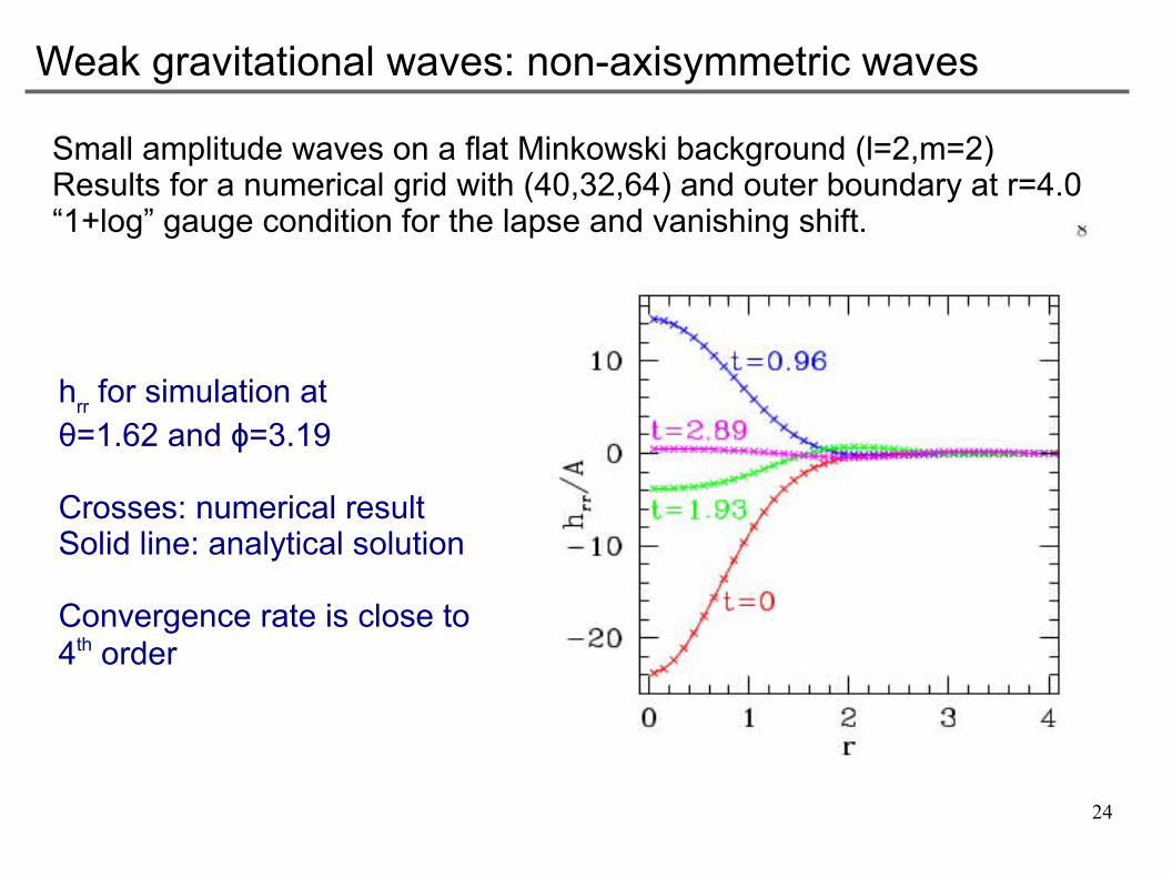
Small amplitude waves on a flat Minkowski background (l=2,m=2)Results for a numerical grid with (40,32,64) and outer boundary at r=4.0“1+log” gauge condition for the lapse and vanishing shift.

25

Hydro-without-hydro: rotating relativistic stars

Stable relativistic star (Γ=2) rotating at 92% of the allowed mass-shedding limit. (M~0.85Mmax and rp/req~0.7)

Results for a numerical grid with (48,32,2) and outer boundary at r=25M“1+log” gauge condition for the lapse and “Gamma-driver” condition for the shift.

Snapshots of the conformalexponent and the lapse at The initial time and aftertwo spin periods along the pole and the equator.

Both profiles remain very similar to the initial data.

26

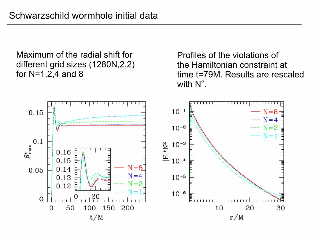
Schwarzschild wormhole initial data

Numerical grid of size (10240,2,2) with outer boundary at r=256M.

Coordinate transition from wormhole initial data to time-independent trumpet data.

We plot conformal exponent, lapse and radial orthonormal component of the shift as a function of the gauge-invariant areal radius R

Conformal factor: Pre-collapsed lapse:

27

Schwarzschild wormhole initial data

Maximum of the radial shift for different grid sizes (1280N,2,2) for N=1,2,4 and 8

Profiles of the violations ofthe Hamiltonian constraint at time t=79M. Results are rescaledwith N2.

28

Collapse of GWs and BH formation using the puncture coordinates:

Collapse of Teukolsky GWs formsa BH that settles to the trumpet solution

Tendicity: the contraction of the electric part of the Weyl tensor with the normal of the horizon

It measures the tidal forces that you would feel on the horizon.

Another application: collapse of GWs

29

€

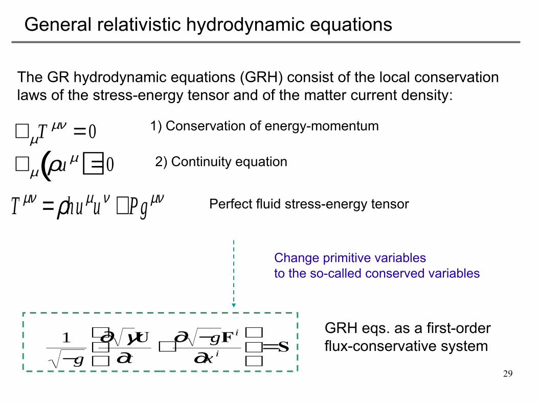
∇µT µν = 0

€

∇µ ρu µ( )=0

Change primitive variablesto the so-called conserved variables

€

T µν =ρh u µu ν + P g µν Perfect fluid stress-energy tensor

1) Conservation of energy-momentum

2) Continuity equation

The GR hydrodynamic equations (GRH) consist of the local conservation laws of the stress-energy tensor and of the matter current density:

€

1

−g

∂ γU∂t

+∂ −gF i

∂x i

=S

GRH eqs. as a first-order flux-conservative system

General relativistic hydrodynamic equations

30

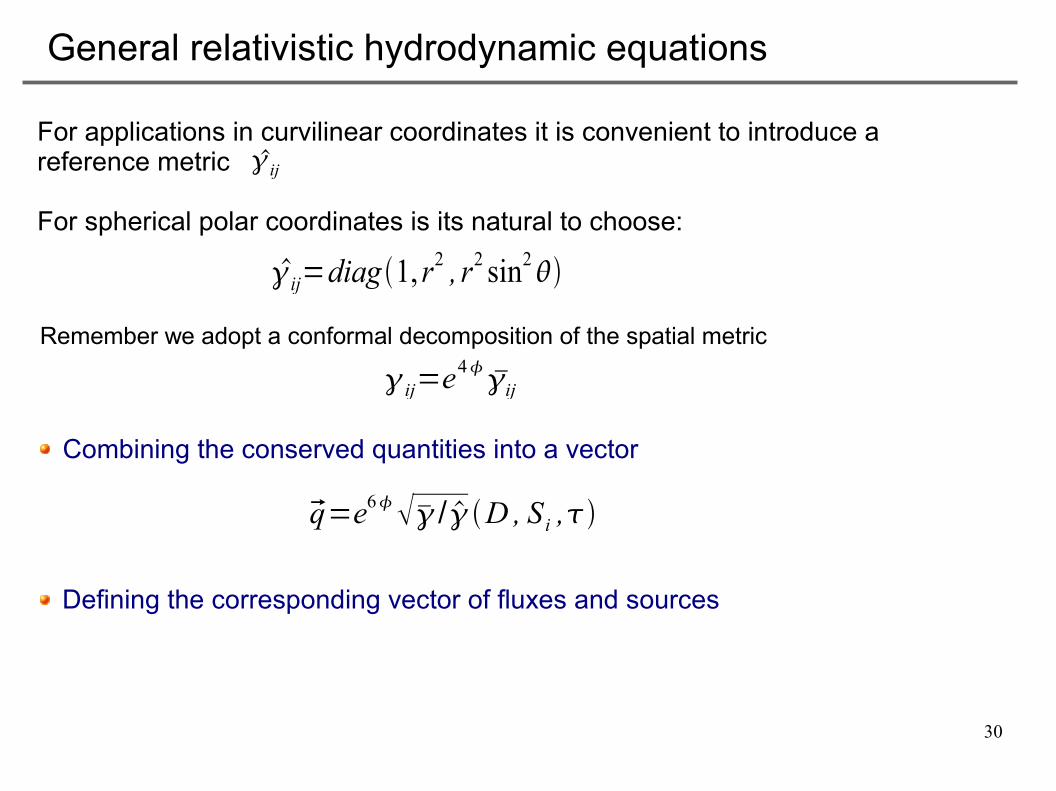
General relativistic hydrodynamic equations

For applications in curvilinear coordinates it is convenient to introduce a reference metric

For spherical polar coordinates is its natural to choose:

ij

ij=diag1, r2 , r2 sin2

Combining the conserved quantities into a vector

Defining the corresponding vector of fluxes and sources

q=e6/ D , S i ,

Remember we adopt a conformal decomposition of the spatial metric

ij=e4

ij

31

∂te6 / S i∂ j f Si

j=S Si f Skj ji

k− f Sik kj

j

=1 ; Di=∂i

We recover the original Valencia formulation by choosing the reference metric to be the flat metric in Cartesian coordinates, so that

∂tq D jf j =s

We can write the GR-Hydro equations in the following form

Note: source terms are also written in terms of covariant derivative associated to the reference metric

For instance, the Euler equations appear as

32

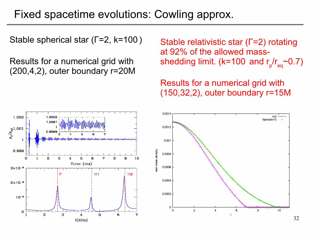
Fixed spacetime evolutions: Cowling approx.

Stable relativistic star (Γ=2) rotating at 92% of the allowed mass-shedding limit. (k=100 and rp/req~0.7)

Results for a numerical grid with (150,32,2), outer boundary r=15M

Stable spherical star (Γ=2, k=100 )

Results for a numerical grid with (200,4,2), outer boundary r=20M

33

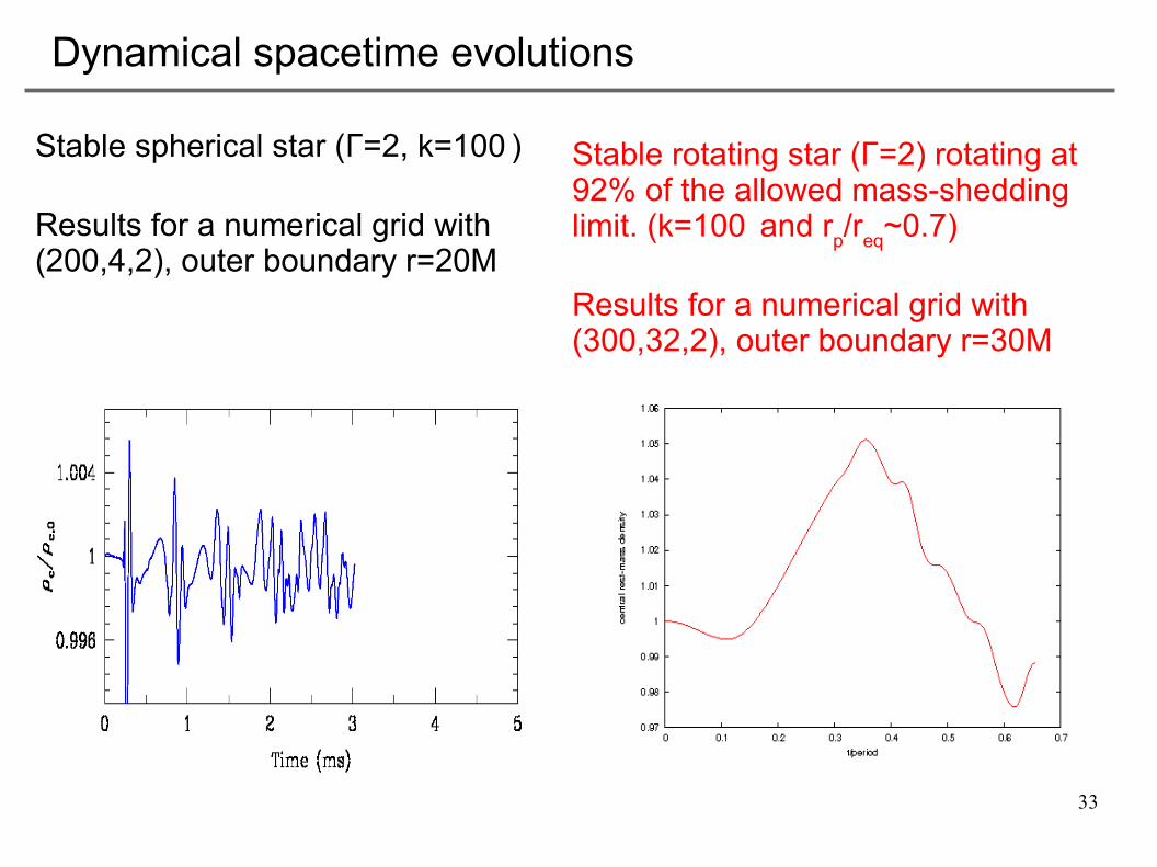
Dynamical spacetime evolutions

Stable rotating star (Γ=2) rotating at 92% of the allowed mass-shedding limit. (k=100 and rp/req~0.7)

Results for a numerical grid with (300,32,2), outer boundary r=30M

Stable spherical star (Γ=2, k=100 )

Results for a numerical grid with (200,4,2), outer boundary r=20M

34

Conclusions

Presented a new numerical relativity code that solves the BSSN equations in spherical polar coordinates without any symmetry assumption.

A key ingredient is the PIRK scheme to integrate the evolution equations in time which allows us to avoid the need for a regularization at the origin or the axis

Obtained the expected stability and convergence of the code

Recent developments:

3D AH finderGR-hydrodynamics (HRSC)GW extraction (Nicolas Sanchis, University of Valencia)Non-uniform grid (Tobias Denk, MPA)