At present, water scarcity is a global challenge affecting every continent around the world. About 11% of the world’s popu-lation currently relies on unimproved drinking water sources [1]. Nearly one-fifth of the global population lives in areas where water is physically scarce [2]. Regionally, the limit of ecological sustainability of water available for abstrac-tion will be exceeded for about half of the human population by 2030 [3]. An analysis of groundwater extraction revealed that depletion rates doubled between 1960 and 2000 and are especially high in parts of India, China, and the United States [4]. Even in a number of European countries (Great Britain, Poland, Spain, Germany, and the Czech Republic), the situa-tion with total renewable water resources is characterized as vulnerable or stressed [5]. About 120 million people in the European region do not have access to safe drinking water [6]. The situation is much worse in sub-Saharan Africa—the region with the most heterogeneously distributed water
resources—where the population is predicted to reach 2.4 bil-lion people by 2050 [7].
About 97.5% of the water reserves on the Earth are stored in easily accessible reservoirs, with around 1.0% being brackish groundwater (0.05–3.0% salts by weight) and the remaining 96.5% being seawater (3.0–5.0% salts) [8]. Thus, the vast amounts of saline water could offer a seemingly unlimited and steady fresh water (<0.05% salts) supply. However, a practical desalination process has to meet several essential requirements such as technological reliability, relative sim-plicity, amenability to large-scale continuous operation, eco-nomic viability, minor impact on the environment, energy efficiency, etc [9]. At present, the most common desalination techniques employed for large-scale purification of seawater and brackish groundwater are thermal desalination (TD) and reverse osmosis (RO), which account together for roughly 90% of desalinated water production. The former technique became commercially available in the 1950s. The minimum energy required to drive TD is directly related to the heat of water vaporization, which is substantially higher than that of other desalination techniques. Although TD requires minimal
Journal of Physics: Condensed Matter
Numerical simulation of electrochemical desalination
D Hlushkou1, K N Knust2, R M Crooks2 and U Tallarek1,3
1 Department of Chemistry, Philipps-Universität Marburg, Hans-Meerwein-Strasse 4, 35032 Marburg, Germany2 Department of Chemistry and the Center for Nano and Molecular Science and Technology, The University of Texas at Austin, 105 E. 24th St., Stop A5300, Austin, TX 78712, USA
Received 15 August 2015, revised 8 February 2016Accepted for publication 10 March 2016Published 19 April 2016
AbstractWe present an effective numerical approach to simulate electrochemically mediated desalination of seawater. This new membraneless, energy efficient desalination method relies on the oxidation of chloride ions, which generates an ion depletion zone and local electric field gradient near the junction of a microchannel branch to redirect sea salt into the brine stream, consequently producing desalted water. The proposed numerical model is based on resolution of the 3D coupled Navier–Stokes, Nernst–Planck, and Poisson equations at non-uniform spatial grids. The model is implemented as a parallel code and can be employed to simulate mass–charge transport coupled with surface or volume reactions in 3D systems showing an arbitrarily complex geometrical configuration.
pre-treatments of the feed water, the commercial use of this desalination technique is limited to geographical regions, such as the Middle East, rich in energy resources. A widely used alternative desalination technique involves RO, which is induced if a hydrostatic pressure differential greater than the osmotic pressure of the feed water is applied across a semi-permeable membrane. The minimum energy required for RO is directly related to the salt concentration of the feed water. With advances in membrane technology and energy recovery devices, RO can nowadays operate with an energy efficiency better than that of any other currently commercialized desali-nation method [10]. However, RO requires extensive pre-treatment of the feed water and product post-treatment due to fragility, contamination, and fouling of the membrane, which greatly increases the production cost of water purified by this technique [10, 11]. In recent years, a number of strategies and approaches have been proposed as alternative routes for water desalination. These novel techniques include microbial desalination [12], the use of carbon nanotube membranes for filtration and RO processes [13], shock electrodialysis [14], desalination by ion concentration polarization [15], water purification with biomimetic aquaporin membranes [16–18], capacitive deionization [19–23], desalination with entropy batteries [24], and gas hydrate-based desalination using new formers [25–27]. Without distinction of the diverse underlying phenomena, a desalination process can be defined as sepa-rating a feed salt solution into deionized water and concen-trated brine streams.
Recently, our groups have shown that electrochemical reactions can be employed for the enrichment and depletion [28–34], separation [35], as well as controlled delivery [36] of charged species from a solution flowing through microchannel systems with embedded electrodes. Each of these applications is based on the principles of electrokinetic equilibrium and dif-ferences between local electromigration, diffusive, and advec-tive fluxes of ions. The key to these techniques is the formation of a localized electric field gradient induced by electrochem-ical reactions at the embedded electrode surfaces. We have discovered these same principles can be employed to desalt seawater by a technique called electrochemically mediated desalination (EMD) [37, 38]. This novel approach provides a number of benefits relative to currently available desalina-tion methods. Firstly, it is membraneless, thereby eliminating major drawbacks of membrane-based desalination technolo-gies: fragility and fouling of membranes and the necessity of intensive pre-treatment of the feed seawater. In contrast, the only pre-treatment required to perform EMD is the sedimen-tation of sand and debris present in seawater [37]. Because of this minimal pre-treatment, considerable cost savings could be provided compared to membrane-based techniques such as RO and electrodialysis. Secondly, EMD is energy- efficient: For 25% salt rejection in seawater at 50% recovery, the energy efficiency is 0.025 kWh m−3 [38]. This value is near the theoretical minimum energy calculated using the same rejection and recovery (about 0.017 kWh m−3). Thirdly, EMD requires only a simple power supply to operate. Therefore, this desalination technique may be employed in settings with a low-voltage battery or renewable energy source without a
high-voltage converter. Finally, the EMD platform may be implemented in a massive parallel format. The last aspect appears to be essential because our basic experimental EMD units are currently realized in microchannel format. However, apart from its parallel implementation, the performance of systems employing this novel desalination technique may be substantially enhanced by an increase in the functional effi-ciency of a single EMD unit. For this purpose, optimization of the geometrical configuration and operating conditions of the EMD unit is required. In this relation, numerical simulations of the phenomena involved in the EMD process are able to provide a better understanding of this desalination technique as well as to maximize the use of resources by replacing phys-ical experiments with computational studies.
In this contribution, we present a numerical approach to simulate the desalination process in the EMD unit. The pro-posed numerical model is based on equations describing the coupled 3D hydrodynamic, mass–charge transport, and electrostatic problems. The model was developed based on numerical schemes with inherent parallelism, allowing the straightforward implementation at modern high-performance computational systems (supercomputers). Results obtained with the proposed simulation approach agree very well with the experimental data we previously reported [37, 38]. The analysis of the simulated data highlights the complex inter-play between the mass–charge transport, hydrodynamics, and electrochemical reactions involved in the EMD process.
2. Experimental EMD unit
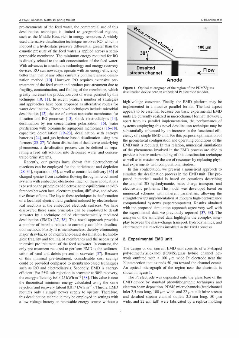
The design of our current EMD unit consists of a Y-shaped poly(dimethylsiloxane) (PDMS)/glass hybrid channel net-work outfitted with a 100 μm wide Pt electrode near the Y-intersection that extends 50 μm toward the channel center. An optical micrograph of the region near the electrode is shown in figure 1.
The Pt electrode was deposited onto the glass base of the EMD device by standard photolithographic techniques and electron beam deposition. PDMS microchannels (feed channel inlet 2.5 mm long, 100 μm wide, and 22 μm tall; brine stream and desalted stream channel outlets 2.5 mm long, 50 μm wide, and 22 μm tall) were fabricated by a replica molding
Figure 1. Optical micrograph of the region of the PDMS/glass desalination device near an embedded Pt electrode (anode).
J. Phys.: Condens. Matter 28 (2016) 194001
D Hlushkou et al
3
procedure. The outlet of the brine stream channel branched from the desalted stream channel at a 30° angle. At each microchannel terminal, a reservoir was made using a 3 mm diameter metal punch to remove PDMS. Finally, a PDMS mold was attached to the glass base by O2 plasma bonding.
Pressure driven flow (PDF) is initiated in the EMD unit by creating a solution height differential in the reservoirs at the ends of the channel by adding or removing seawater. A power supply is used to apply a low-voltage bias between the microfabricated Pt anode and grounded electrodes (cath-odes) dipped into the reservoirs. Applied voltage is adjusted to a value (a few volts) that results in electrochemical reaction at the anode—the oxidation of chloride ions (Cl−) present in seawater:
−− −2Cl 2e Cl .2→ (1)
This reaction leads to the formation of an ion depletion zone (region of high solution resistivity) near the anode, thus pro-ducing a local electric field gradient and providing a means for controlling the movement of ions. As a result, a seawater feed is separated into brine and desalted water streams at the junction of the branched channel.
3. Theoretical background and numerical approaches to modeling EMD
In this section we present the theoretical model and the com-putational methods used to simulate the basic EMD process. The 3D geometry of the modelled system is exactly the same as that used for the experiments (see figure 1) and is shown in figure 2.
All microchannels are terminated by macroscopic reser-voirs containing the grounded electrodes (cathodes). As model liquid we used a 0.55 M aqueous NaCl solution (which reflects the Cl− concentration in seawater) and furthermore assume that Cl− is oxidized at the embedded electrode (anode). The computer model simulates stationary PDF initiated in the microchannel system as well as the stationary distributions of local ion concentrations and local electric field strength. In fact, in an aqueous NaCl solution the ionic species include Na+, Cl−, H3O+, and OH−. However, in a 0.55 M solution of NaCl, the concentration of hydronium and hydroxide ions is
much lower than that of the sodium and chloride ions. This allows us to consider only Na+ and Cl− ions as the species of interest in the modelled system.
In seawater and an aqueous NaCl solution there are two major species that can be oxidized at the anode: Cl− and water. However, in the electrolysis of seawater and a concen-trated NaCl solution, Cl− oxidation is the preferred anodic process over water oxidation. The main reasons leading to the predominance of Cl− oxidation at the anode are reported as follows [39–43]:
(i) Local acidification of the electrolyte near the anode increases the thermodynamic potential for oxygen evol-ution, favouring chloride oxidation since it is independent of the pH.
(ii) The overpotential for chloride oxidation is lower than that for the oxidation of water.
(iii) Oxygen evolution is a slow electrochemical process with low exchange current density. The ratio of the exchange current densities for chlorine and oxygen evolution at most anode materials is in the range of 103–107. This ratio characterizes the ease of chlorine evolution relative to oxygen.
Therefore, the assumption that all of the current conducted through the anode results in only oxidation of Cl− ions is accurate to a very good approximation for the studied system.
Taking the liquid as incompressible, the local flow velocity field (v) can be described by the Navier–Stokes equation
⎜ ⎟⎛⎝
⎞⎠ρ η
∂∂+ ⋅∇ = −∇ + ∇
tp
vv v v,2 (2)
where ρ and η are the mass density and dynamic viscosity of the liquid, and p is hydrostatic pressure. It should be men-tioned that the above equation does not contain the electric body force term which accounts for the contribution of elec-troconvection to charge transport. Generally, there are two modes of electroconvective phenomena eventually observed in an electrolyte solution [44–46]. The first mode is a result of the action on a macroscopic scale of the electric field upon the residual space charge. The second mode (electroosmotic flow) pertains to the electrolyte slip resulting from the action of the tangential (relative to the solid–liquid interface) component of the electric field upon the space charge of the electric double layer. Though electroconvection may change significantly the spatiotemporal ion distributions in systems with charge-selective domains (such as metallic electrodes, ion-exchange membranes or nanochannels), its effect under the operating conditions in the system we modelled (with a 0.55 M elec-trolyte solution and a 50 nA current through the electrode) is negligible [44, 47–50]. We return to this issue in section 4 when we discuss the simulation results.
Bulk spatiotemporal variations in the concentrations of Na+ and Cl− ions are governed by balance equations
φ∂∂= −∇ = ∇ + ∇ − ∇
n
tD n n
F
RTD nj vNa
Na Na2
Na Na Na2
Na
(3)and
Figure 2. Schematic of the microchannel system used for simulation of the EMD device. The thickness (Z-dimension) of the microchannels is 22 μm.
J. Phys.: Condens. Matter 28 (2016) 194001
D Hlushkou et al
4
φ∂∂= −∇ = ∇ − ∇ − ∇
n
tD n n
F
RTD nj v,Cl
Cl Cl2
Cl Cl Cl2
Cl
(4)where n is the species volume concentration (m−3), j is the flux, D is the diffusion coefficient, and φ denotes the local electric potential; F, R, and T represent the Faraday constant, molar gas constant, and temperature, respectively.
The Poisson equation establishes the essential relationship between the local ionic concentrations of the species and the local electric potential
φε ε
∇ = −−
qn n
,2e
Na Cl
0 r (5)
where qe is the elementary charge; ε0 and εr are the vacuum permittivity and dielectric constant of the liquid. In (2)–(5) it is assumed that the mass density, viscosity, diffusion coef-ficients, and dielectric constant are independent of the ion concentration.
Instead of a direct numerical resolution of the Navier–Stokes problem (2), the simulation of hydraulic flow through the microchannel system was performed using the lattice-Boltzmann equation (LBE) method, a kinetic approach that operates with discrete space and time [51–53], where the macroscopic fluid dynamics is approximated by the motion of (and interactions between) fictitious particles on a regular lattice. This approach is based on the idea that the resulting fluid flow is determined mainly by the collective behaviour of molecules and not by their detailed interactions. Each of the fictitious particles is then already associated with ‘a large number’ of fluid molecules. Specifically, the LBE can be regarded as a finite-difference approximation of the Boltzmann equation, which is obtained by its truncation in a Hermite velocity spectrum space [52, 54]. Among the advantages of the LBE method are its inherent algorithmic parallelism as well as its capability to handle solid–liquid interfaces with complex geometry, e.g. in disordered porous media [51].
The kinetics of a fluid in terms of a statistical system can be described with a distribution function F(r, u, t) such that F(r, u, t)drdu is the number of fluid particles which, at time t, are located between r and (r + dr) and have velocities in the range from u to (u + du). Then, the density ρ of the fluid and its velocity v can be obtained by momentum integration of this distribution function
( ) ( )∫ρ =t M F tr r u u, , , dm (6)
and
( )( )
( )∫ρ=t
tM F tv r
ru r u u,
1
,, , d ,m (7)
where Mm is the mass of a particle. The spatiotemporal changes in the distribution function can be described by the following evolution equation
( ) ( )+ + + = +Ω⎛⎝⎜
⎞⎠⎟F t
Mt t t F t F tr u u
fr u r u r ud , d , d d d , , d d d ,
m (8)
where f is the acting external force and Ω is the collision operator. Appropriate choice of the collision operator allows to determine accurately the macroscopic properties of a fluid, since these are not directly dependent on the details of the microscopic behaviour but mainly defined through interac-tions between particles. This offers the transition toward a simplified dynamics with discrete space, time and molecular velocities. In particular, the discrete analogy of (8) is
δ δ+ + = +Ωα α α α αF t t t F t Fr e r, , ,( ) ( ) ( ) (9)
where Fα is the distribution function for the αth discrete velocity eα at position r and time t, and δt is the time step used in the LBE simulation. Here, we implemented the lattice-BGK (Bhatnagar–Gross–Krook) model [52], a modification of the LBE method characterized by a single-time relaxation collision operator
δ δτ
+ + = + −α α α α αF t t t F t F t F tr e r r r, ,1
, , ,eq( ) ( ) [ ( ) ( )] (10)
where αFeq represents the equilibrium distribution function and τ is a non-dimensional relaxation time. This parameter is con-nected with the kinematic viscosity (κ) of the fluid by
κτ
=−2 1
6.
(11)
The values of velocities eα in (9) and (10) are chosen such that during one time step δt each particle moves from one lat-tice node to its neighbour. In this work, we adapted the D3Q19 lattice, a cubic lattice that can be obtained by projecting the 4D face-centred hypercubic lattice onto 3D space [56, 57]. The D3Q19 lattice has 18 links at each lattice node; each lat-tice node is connected to its six nearest and twelve diagonal neighbours. Particles can move along the 18 links (α = 1–18) or stay at the node (α = 0).
The equilibrium distribution function depends on the local density ρ(r, t) and local velocity v(r, t)
( ) ( )⎡
⎣⎢
⎤
⎦⎥ρ= +
⋅+
⋅−⋅
α αα αF t wc c c
re v e v v v
, 12 2
eq
S2
2
S4
S2 (12)
where cS is the speed of sound and wα is a weighting factor that is governed by the length of the velocity vector eα. With the D3Q19 lattice, these factors are as follows: wα = 1/3 for α = 0, wα = 1/18 for α corresponding to lattice links to the nearest neighbours, and wα = 1/36 for α corresponding to lat-tice links to the diagonal neighbours. The lattice spacing (Δh) we used for the simulation of the PDF velocity field was set to 1.0 μm. At the solid–liquid (microchannel wall–electrolyte solution) interface, a halfway bounce-back rule was applied to implement the required ‘liquid-stick’ velocity boundary con-dition [58].
The Poisson and Nernst–Planck equations (3)–(5) were resolved with conventional finite-difference methods. For this purpose, the solution domain was split into a set of equal cubic cells with a size of Δh = 1.0 μm (generating a uniform cubic grid). The electric potential and ion concentrations are deter-mined at the center points of the cells. The spatiotemporal finite-difference scheme for solution of the Nernst–Planck
J. Phys.: Condens. Matter 28 (2016) 194001
D Hlushkou et al
5
equations (3, 4) is based on the calculation of the total flux in a cell, thereby accounting for the flux components on each of the six cell surfaces (figure 3).
Then, (3) and (4) can be represented, respectively, as
∂∂= −∆
− + − + −+ − + − + −n
t hj j j j j j
1X X Y Y Z Z
NaNa, Na, Na, Na, Na, Na,( )
(13)and
( )∂∂= −∆
− + − + −+ − + − + −n
t hj j j j j j
1.X Y Y Z Z
ClCl, Cl,X Cl, Cl, Cl, Cl,
(14)
By introducing the discrete time step Δt, the two above equa-tions can be written as
( )= −∆∆
− + − + −+∆ + − + − + −n nt
hj j j j j jt t t
X X Y Y Z ZNa Na Na, Na, Na, Na, Na, Na,
(15)and
= −∆∆
− + − + −+∆ + − + − + −n nt
hj j j j j j ,t t t
X X Y Y Z ZCl Cl Cl, Cl, Cl, Cl, Cl, Cl,( ) (16)where nt and nt+Δt are the species concentrations at time t and (t + Δt), respectively.
A finite-difference approximation of a particular (X-)
component of the ion flux +jX k l m, , , in a cell with discrete co-ordinates k, l, m (corresponding to X-, Y-, and Z-directions, respectively) is
φ φ
=−∆
±+ −
∆
−+ +
+ +
+ +
+ +
j Dn n
hFD
RT
n n
hn n v v
2
2 2
X k l mk l m k l m
k l m k l m k l m k l m
k l m k l m X k l m X k l m
, , ,, , 1, ,
, , 1, , , , 1, ,
, , 1, , , , , , 1, ,
(17)
where vX is the X-component of the flow velocity field. The sign before the second term on the rhs of (17) is determined by the valence of the species: it is ‘ + ’ and ‘ − ’ for Na+ and Cl− ions, respectively. Expressions similar to (17) can be derived for all other flux components. If a cell is adjacent to the channel wall, the corresponding terms in (15) and (16) become zero.
A special treatment is used for cells adjoining the embedded electrode. The region near the electrode is char-acterized by steep gradients of the electric field strength and ion concentrations. As a result, the spatial resolution of 1 μm cannot assure a good accuracy with the use of a finite-differ-ence approximation. To resolve this problem, we introduce a locally non-uniform grid: Each cell adjoining the electrode (a ‘parent’cell) is split into I sub-cells (‘child’ cells or layers) with dimension of Δh = 1.0 μm along X- and Y-directions (tangential to the electrode surface) and an exponentially decreasing thicknesses, Δhi, along the Z-direction toward the electrode (figure 4).
For the current study, we split such cells into 20 sub-cells (i = 1, …, I; I = 20). The largest value of the index i = 20 corresponds to the sub-cell (layer) which is adjacent to the electrode surface. The thickness Δhi of the ith sub-cell is determined as
∆ = ∆ = −∆ = ∆ =
−
−
h h i Ih h i I
2 if 1,..., 1if .
ii
i i 1 (18)
Specifically, with I = 20 the smallest value of Δhi is about 1.9 × 10⁻⁶ μm, which allows us to achieve an accurate finite-difference approximation of the gradient operators for the electric field strength and ion concentrations. Below, we denote the discrete co-ordinates of a sub-cell with thickness Δhi as k, l, m, i, where k, l, m are the discrete co-ordinates of the ‘parent’cell that is split into ‘child’ sub-cells.
Figure 3. Denotation of the flux components in a cubic cell employed to resolve the Nernst–Planck equation by a finite-difference scheme.
Figure 4. Illustration of the non-uniform spatial grid employed for resolving the Nernst–Planck (and Poisson) equation with finite-difference schemes. A cell adjoining the electrode (red) is split into sub-cells (layers) with exponentially decreasing thickness. For this study, such cells were split into 20 layers.
J. Phys.: Condens. Matter 28 (2016) 194001
D Hlushkou et al
6
Accounting for the difference between the thicknesses of adjoining sub-cells, the finite-difference approximations of
flux components +jZ k l m i, , , , and −jZ k l m i, , , , (see figures 3 and 4 and (17)) can be written as
φ φ
=−
∆ +∆
±+ −
∆ +∆
−+ +
+ −
−
− −
−
− −
j Dn n
h h
FD
RT
n n
h hn n v v
0.5
2 0.5
2 2
Z k l m ik l m i k l m i
i i
k l m i k l m i k l m i k l m i
i i
k l m i k l m i Z k l m i Z k l m i
, , , ,, , , , , , 1
1
, , , , , , 1 , , , , , , 1
1
, , , , , , 1 , , , , , , , , 1
( )
( )
(19)
and
( )
( )φ φ
=−
∆ +∆
±+ −
∆ +∆
−+ +
− +
+
+ +
+
+ +
j Dn n
h h
FD
RT
n n
h hn n v v
0.5
2 0.5
2 2.
Z k l m ik l m i k l m i
i i
k l m i k l m i k l m i k l m i
i i
k l m i k l m i Z k l m i Z k l m i
, , , ,, , , , , , 1
1
, , , , , , 1 , , , , , , 1
1
, , , , , , 1 , , , , , , , , 1
(20)
In these equations, the sign before the second term on the rhs is determined by the valence of the species, as specified for (17). Expressions similar to (19) and (20) are applied also to calculate the flux Z-component in neighbouring ‘parent’and ‘child’cells by setting Δhi = Δh for a ‘parent’ cell.
In the proposed numerical approach to resolve the Nernst–Planck equation, the occurrence of the electrochemical reac-tion (1) is accounted for through the flux component −jZ k l m I, , , , for Cl− ions. This term determines the decrement of the Cl− concentration due to oxidation at the anode surface and for sub-cells with discrete co-ordinates k, l, m, I becomes
=−jI
Sq,Z k l m I, , , ,
el
e (21)
where Iel denotes the current through the electrode and S is the area of the electrode surface in contact with the electrolyte solution (see figures 1 and 2).
A similar numerical approach is employed to resolve the Poisson equation (5). Its basic finite-difference approximation is
(
)
φ φ φ φ φ
φ φε ε
∆+ + + +
+ − = −−
+ − + − +
−
h
qn n
1
6
k l m k l m k l m k l m k l m
k l m k l mk l m k l m
2 1, , 1, , , 1, , 1, , , 1
, , 1 , , eNa, , , Cl, , ,
0 r
(22)
or
( )φε ε
φ φ
φ φ φ φ
=∆
− + +
+ + + +
+ −
+ − + −
⎡
⎣⎢
⎤
⎦⎥
q hn n
1
6
.
k l m k l m k l m k l m k l m
k l m k l m k l m k l m
, ,e
2
0 rNa, , , Cl , , , 1, , 1, ,
, 1, , 1, , , 1 , , 1
(23)
For cells adjacent to the anode surface, we use the same ‘split-ting’ procedure described above. A finite-difference approx-imation of the Poisson equation for neighbouring cells with distinct values of their thickness (Z-dimension) is
( )ϕ ϕ φ φ ϕ
φ φ
ϕ ϕ
ε ε
∆+ + + −
+∆ +∆
−
∆ +∆
−−
∆ +∆=
−
+ − + −
+ −
−
−
+
+
⎛⎝⎜
⎞⎠⎟
h
h h h h
h hq
n n
14
4
.
k l m i k l m i k l m i k l m i k l m i
k l m i k l m i
k l m i k l m i
i i
k l m i k l m i
i i
k l m i k l m i
2 1, , , 1, , , , 1, , , 1, , , , ,
, , , 1 , , , 1
, , , 1 , , ,
1
, , , , , , 1
1e
Na, , , , Cl, , , ,
0 r
(24)
For sub-cells adjoining the electrode surface, the electric potential φk,l,m,I is adjusted to φel, the potential of the anode relative to the one in the inlet and outlet reservoirs.
The program realization of the presented numerical approach to resolve the Navier–Stokes, Nernst–Planck, and Poisson equations was implemented as parallel code in C/C++ language using the message passing interface (MPI) standard [59]. After discretization of the modelled system, the resulting spatial grid was composed of ~107 nodes. At the first stage, the 3D flow velocity field was computed using the LBE approach. Then, the coupled Nernst–Planck and Poisson equations were resolved with the presented finite-difference schemes. All simulations were performed on SuperMUC, a supercomputer at the ‘Leibniz-Rechenzentrum der Bayerischen Akademie der Wissenschaften’ (LRZ, Garching, Germany). The final (productive) simulation reported and analyzed in this work required roughly 6 h at 1024 processor cores.
4. Results and discussion
The 3D numerical approach described in section 3 was subse-quently employed to simulate the EMD process in the micro-channel system presented with figures 1 and 2. The simulation has mirrored the experiment carried out for the desalination of a 0.55 M aqueous NaCl solution with a current through the embedded electrode of 50 nA, a volumetric PDF rate of 0.1 μl min−1, and an electrode potential of 0.9 V. The dynamic viscosity and mass density of the NaCl solution was 0.966 mPa s and 1.023 × 10³ kg m−3, respectively. Diffusion coefficients were adjusted to 1.334 × 10⁻⁹ and 2.033 × 10⁻⁹ m2 s−1, for Na+ and Cl− ions, respectively. The temperature of the system was set to 293.16 K.
Fully developed, stationary PDF in the modelled EMD system is required as transport mechanism for the bulk liquid phase (electrolyte solution). It can be conveniently generated by introducing and maintaining different heights of electro-lyte solution levels at the terminating ends of the respective microchannels. This results in steady-state Hagen–Poiseuille flow in the microchannel, feeding the bulk electrolyte solution towards the Y-intersection, i.e. the microchannel branch. The flow is characterized by a 3D channel cross-sectional velocity profile that closely resembles the classical parabolic velocity profile in a cylindrical pipe. That is, flow velocity increases from zero at the channel walls, where the no-slip velocity boundary condition prevails (as implemented in the simula-tions), to a maximum in the center of the channel cross-sec-tion. However, in contrast to the classical cylinder geometry, the four corners of the rectangular microchannel geometry present additional low-velocity regions (with corresp onding
J. Phys.: Condens. Matter 28 (2016) 194001
D Hlushkou et al
7
hydrodynamic boundary layers) due to the abrupt changes in local curvature of the solid–liquid interface. This has been observed before with LBE-based 3D simulations of laminar flow through noncylindrical conduits [55]. When the flow approaches the Y-intersection further downstream in the feed microchannel, the velocity profile becomes disturbed by the diverging branch geometry and unsymmetric. Figure 5 illustrates that situation with the X-component of the simu-lated flow velocity field in the microchannel system near the Y-intersection. The actual volumetric flow (0.1 μl min−1) through the channel (100 μm width × 22 μm height) trans-lates into a Reynolds number (Re), characterizing the relative importance of inertial and viscous forces, of Re = vavdhρ/η ~ 0.03. This low value is obtained using the resulting average velocity (vav = 0.76 mm s−1), the hydraulic channel diam-eter (dh = 36 μm), and the kinematic viscosity of the liquid (η /ρ = 9.443 × 10⁻⁷ m2 s−1) and is characteristic of the creeping flow regime (Re < 1), where inertial effects can be ignored in comparison to the viscous resistance.
In all regions of the modelled EMD system, except near the Y-intersection and the channel walls, in general (including the channel corners with their hydrodynamic boundary layers), the transport of ions is advection-dominated by the PDF. However, if this advection were the only transport mech-anism, then ions in bulk solution could not be delivered in a preferential direction at the Y-intersection, where the feed microchannel branches. This situation merely corresponds to a stream-splitting with identical composition of the two resulting (splitted) streams. In fact, net transport of ionic
species present in the modelled system in longitudinal and transverse directions with respect to the feed microchannel axis results from the superposition of advection, diffusion, and migration. The latter is determined, in particular, by the local electric potential gradient developing in the coupled electro-chemical module (realized through the embedded anode), which in turn depends on the local ion concentrations. Since the electric field gradient is a key to EMD device functionality it is described in more detail.
Thus, the next step beyond the relatively simple situation illustrated by figure 5 (with pure PDF) is the onset of oxidation of Cl− ions. This produces electroneutral chlorine molecules and therefore reduces the number of ionic charge carriers near the embedded anode. It is a straightforward electrochemical process that occurs locally but steadily and, together with the diffusion and migration of the ions in the system as well as the superimposed PDF, after some time results in a steady-state depleted concentration polarization zone with an associated electric field gradient. We have experience with in situ formed localized electric field gradients for enrichment, depletion, sep-aration, and controlled delivery of charged species from a solu-tion flowing through microchannel systems [28–36]. Key to these techniques is the formation of a localized electric field gra-dient induced through electrochemical reactions at embedded electrode surfaces. In this regard, we have discovered that the same principles can be employed to desalt seawater.
Based on experimental data for steady-state electric cur-rents in our EMD device [37], we can calculate the charge passed through the embedded anode and therefore, assuming all that current goes toward the oxidation of Cl− ions (justi-fied in the beginning of section 3), estimate the amount of chloride oxidation. This analysis, reported in detail in the sup-porting information of [37], reveals that only ~0.01% of the total Cl− ions present in solution is oxidized. That is, only 1 out of 10 000 chloride ions passing through the microchannel cross-section at a time is oxidized at the embedded anode; the remaining 9999 Cl− ions, wherever they are located in the cross-section, are unaffected regarding their oxidation state and trajectory governed by the fluid flow field (figure 5). However, due to the reduced number of ionic charge car-riers at and near the embedded anode (electroneutral chlo-rine molecules are produced from chloride ions), a diffusive flux of Cl− ions from the center of the channel toward the surface of the anode, perpendicular to the streamlines of the laminar PDF, develops in the effort to compensate the loss of Cl− ions caused by the electrochemical reaction. At steady-state regarding the local electrochemical consumption of Cl− ions, their diffusive flux normal to the anode surface, and the superimposed PDF, a considerably streamlined depleted con-centration polarization zone (extended advection-diffusion solid–liquid boundary layer) is expected to form. Without PDF this situation will reduce to a diffusion boundary layer, which propagates until the depleted concentration polariza-tion zone reaches the external reservoires. All this conforms to the classical picture of concentration polarization near a metal–liquid electrolyte interface (with or without superim-posed flow), at which a charged species is either generated or consumed with a constant rate [60].
Figure 5. Distribution of the X-component of the simulated flow velocity in the central plane (Z = 11 μm) of the EMD simulation setup near the junction of the branched microchannels. The volumetric flow rate is 0.1 μl min−1.
J. Phys.: Condens. Matter 28 (2016) 194001
D Hlushkou et al
8
We note here that the formation of the depleted concentra-tion polarization zone and its application to seawater desalina-tion using a bifurcated channel design reflects the operational principle in the microchannel device reported by Kim et al [15]. However, compared to our EMD device with ideal permselectivity of the metal–liquid electrolyte interface, they utilized a Nafion membrane with nonideal cation-selectivity to create the ion depletion region.
In the EMD device, the local electrolyte properties near the embedded anode are characterized by a decreased ionic strength. Once the depleted concentration polarization zone is developed (representing higher local solution resistivity), a much larger-than-average amount of the externally applied voltage is dropped in this region, which results in a locally elevated electric field strength. Figure 6 shows the simulated distribution of the Y-component of the electric field near the feed microchannel branch. Simulation results depicted in that figure confirm that oxidation of Cl− ions, which produces electroneutral chlorine molecules, results in a steady-state ion concentration depletion zone and a corresponding increase in local electric field strength. The presence of the field gradient (with respect to figure 5) will result in a stationary redirec-tion of both cationic and anionic species, present in the feed solution, to produce splitted streams with reduced (desalted stream) and increased (brine stream) ionic strength behind the microchannel branch. To interpret the effect of the elec-tric field gradient revealed by figure 6, we take a look at the steady-state distributions of sodium and chloride ions in the modelled system.
These distributions for Na+ and Cl− ions are shown in figure 7. They demonstrate that the ions slow down and accumulate as they approach and initially enter the depleted concentration polarization zone with the associated field gradient (see figure 6). In this border region (with bulk solu-tion) of the advection-diffusion boundary layer, diffusion dominates locally over both migration and the PDF regarding the transport of ionic species. Consequently, the diffusion of Na+ and Cl− ions along their developed concentration gra-dients in all directions also results in a lateral displacement which, together with the PDF, moves a fraction of the ions into the brine channel. The original oxidation of Cl− ions at the embedded anode is needed to create the depleted concen-tration polarization zone, which in turn slows down the ionic transport locally. However, the presence of the PDF is impor-tant in moving apart those ions, which have been successful in diffusing sufficiently away (laterally) in response to the developed zones of increased ionic concentrations (figure 7). Due to the independent (uncorrelated) effects of maintaining the depleted concentration polarization zone and transport by the PDF, the final amount of ions that will be deflected into the brine channel cannot be directly related to the amount of Cl− ions oxidized at the embedded anode.
Figure 8 complements this picture with the simulated steady-state distribution of local salinity in the EMD system under the indicated operating conditions, normalized by the salinity at the inlet of the feed microchannel (which, for the model feed solution used here, is 0.55 M). As can be seen in figure 8, the average reduction of salinity in the desalted
stream is on the order of 20%. This result is similar to the desalting efficiency retrieved in the experiments (25 ± 5%), representing an EMD system operation under comparable conditions [37, 38]. One potential reason for the above (small) difference between experimental and simulated values can be the utilization of the boundary condition (21), which assumes that the current through the anode is a predefined parameter of the model. We are currently developing a modification of the presented numerical model, using the Butler–Volmer equa-tion to determine the local current density through the anode surface as a function of the electrode potential, the standard potential of (and transfer coefficient for) the oxidation reac-tion, and the corresponding exchange current density.
Importantly, our simulations revealed that the electrolyte solution remains electroneutral in the entire system, as evi-denced with the identical distributions for Na+ and Cl− ions in figure 7, except for a very thin electrolyte layer (~0.5 nm) adjoining the anode. The thickness of this layer is comparable with that of the electric double layer formed in a 0.55 M 1:1 electrolyte solution near the electrified solid surface. This is a clear indication that under the operating conditions in our system no extended space charge region (SCR) is formed. The development of the SCR and associated electroconvective instability are used, in particular, to explain the overlimiting-current region of the voltage–current curves for ion-exchange membranes. This instability can lead to the destruction (due to spontaneous development of a vortical flow) of the diffusive
Figure 6. Distribution of the Y-component of the electric field strength near the junction of the branched microchannels. Simulations use a 0.55 M NaCl solution (reflecting the Cl− concentration in seawater) at a volumetric flow rate of 0.1 μl min−1 and an electric current through the electrode of 50 nA at an electrode potential of 0.9 V. (a) Distribution in the central plane (Z = 11 μm) of the device. (b) Distribution in the A–B cross-section of the device.
J. Phys.: Condens. Matter 28 (2016) 194001
D Hlushkou et al
9
layer formed near the membrane surface as a result of the balanced electromigration-diffusion fluxes and, as a con-sequence, to an additional ion transport mechanism in this region. The absence of the SCR under the operating condi-tions in the system we modelled allows to conclude that this additional electroconvective transport mechanism does not occur in the studied system.
Moreover, by a detailed numerical analysis of the electro-convective stability problem, it was shown [45, 49, 50] that neither bulk electroconvection nor equilibrium electroosmosis can yield hydrodynamic instability in concentration polariza-tion in a system with planar geometry and a perfectly charge-selective solid (like a metal electrode). Returning to the Navier–Stokes equation (2) we used to model flow, these two arguments allow to conclude that the presented form of this equation (without electroconvective term) is a quite accurate approximation to reproduce all the relevant convective mech-anisms observed in the system under consideration. Here, it should be mentioned that bulk electroconvective instability can still exist in systems containing charge-selective spatial domains such as ion-exchange membranes or nanochannels, which are inherently not perfectly charge-selective, under conditions resulting in the development of the SCR [61–65]. In addition, it has been shown by direct visualization based on confocal laser scanning microscopy [66] that the presence of PDF can suppress microvortex generation and electrocon-vective instability (see figures 7(b) and 10 in [66]). This may serve as experimental support for justifying the absence of vortex formation and convective instability in our EMD study.
Figure 7. Distribution of the Na+ and Cl− ion concentrations near the junction of the branched microchannels. Concentration in the feed electrolyte solution: 0.55 M, volumetric flow rate: 0.1 μl min−1, electric current through the electrode: 50 nA, electrode potential: 0.9 V. (a) Distribution in the central plane (Z = 11 μm) of the device. (b) Distribution in the A–B cross-section of the device.
Figure 8. Distribution of the solution salinity normalized by the microchannel inlet value (0.55 M in the feed electrolyte solution). Volumetric flow rate: 0.1 μl min−1, electric current through the electrode: 50 nA, electrode potential: 0.9 V. (a) Distribution in the central plane (Z = 11 μm) of the device. (b) Distribution in the A–B cross-section of the device.
J. Phys.: Condens. Matter 28 (2016) 194001
D Hlushkou et al
10
Furthermore, the rationale behind the region with the locally increased electric field strength near the anode, as observed in figure 6, can be motivated by a theoretical approach [45, 67]. Using this approach we can determine the steady-state spatial distribution of the electric field strength in a 1D system (elec-trolytic cell) composed of two plate electrodes separated by a distance d and flanking an aqueous solution of a symmetric monovalent electrolyte. It is assumed that under the applica-tion of the voltage φel across the electrodes electrochemical reactions are initiated, which result in a steady-state ionic flux through the system. Importantly, this theoretical model assumes local electroneutrality of the electrolyte solution. Then, the associated electric field distribution E(x) in the 1D system (0 ⩽ x ⩽ d) can be determined as
( )( / )
=+ −
E x J
RT
Fd J x d2
1
1 2 1, (25)
where
( / )( / )φφ
=− −+ −
JF RT
F RT
1 exp 2
1 exp 2.el
el (26)
Figure 9 shows the distribution of electric field strength cal-culated according to the above 1D theoretical approach, using d = 2.5 mm (which is approximately equal to the dis-tance between anode and the cathodes in the 3D system that we modelled) and φel = 0.9 V (the potential difference in the modelled system).
The theoretical results presented in figure 9 demonstrate that electric field strength in a 1D system with the distance between the electrodes and the electrode potential difference adapted to their values in the modelled 3D system is also very non-uniform. Similar to the simulation results shown in figure 6, the local electric field strength is almost zero already after a distance from the anode of about 100 μm. Electric field strength in the electrolyte region close to the anode, determined with the theoretical model (~25 kV m−1), is even stronger than obtained in our simulations (~15 kV m−1) under similar conditions (d = 2.5 mm, φel = 0.9 V). The difference
between these values can be attributed to the presence of PDF in the EMD system, which contributes to the transport of charged species. The relative importance of contrib utions due to advection and diffusion is characterized by the Péclet number, Pe = vavdh/D. The actual volumetric flow rate (0.1 μl min−1) in the modelled system results in Pe = 13.5 and 20.6 for Cl− and Na+ ions, respectively. Following on a theoretical analysis, it was shown [68] that for Pe > 1 the elec-tric field strength distribution close to an ion-selective surface changes significantly compared to the situation without PDF.
Therefore, both the 1D theoretical approach and the 3D numerical simulations suggest that under similar conditions (d = 2.5 mm and φel = 0.9 V) the electric field in the electro-neutral electrolyte region near the anode (with a thickness of ~50 μm) is much stronger than in the bulk electrolyte solution, even without requiring the formation of an extended SCR.
The local ion concentration distribution at and near the embedded anode, which represents a depleted concentration polarization zone, and the resulting electric field gradient are locally blurred by species diffusion (relaxing concentration gradients) and considerably streamlined by the superimposed PDF, as evidenced by figures 6 and 7. Especially towards the microchannel center (approaching higher PDF veloci-ties), longitudinal advection displaces and flattens the electric field gradient with respect to the underlying sharp position of the anode (dashed square in figure 6(a)) and the higher field strengths conserved in the low-velocity regions of the channel corners. This shows that the PDF rate selected for desalina-tion is an important parameter regarding shape and distribu-tion of the electric field gradient and, therefore, the achievable desalting efficiency with this device under a given set of con-ditions. As illustrated by figure 8(b), the currently employed parameters (e.g. placement of the anode, flow rate, channel geometry and channel dimensions) result in a still significant ‘leakage’ of salinity above the anode into the desalted stream, which partly explains the low desalting efficiency of ~20%. This suggests that an optimal flow rate exists for a given elec-trode configuration, which points to a complex optimization problem regarding desalting efficiency and water recovery at a systematically varied electrode design.
At this point, we emphasize that the minimum energy required to drive the microchannel-based EMD platform is governed by the energy needed for local Cl− oxidation, which produces the depleted ion concentration polarization zone (advection-diffusion boundary layer) and electric field gra-dient (figure 6) responsible for redirection of ionic species in the bypassing electrolyte solution. Importantly, EMD is nei-ther based on a reduction of salinity via direct electrochemical neutralization of ions nor on the local separation of oppositely charged ions (as mentioned above, electrolyte solutions in brine and desalted stream channels remain electroneutral). Instead, the Cl− oxidation-based generation of the depleted concentration polarization zone, which is responsible for the locally increased ion concentrations near its border with the bulk electrolyte solution due to the diffusion-limitation that takes effect in this boundary layer (figure 7), and the actual removal of ions, which have diffused laterally in the micro-channel as a consequence of these locally increased ion
Figure 9. Distribution of electric field strength in a 1D electrolytic cell as a function of the distance from the anode according to the theoretical approach developed in [45] and [67]. Distance between electrodes: 2.5 mm, electrode potential: 0.9 V.
J. Phys.: Condens. Matter 28 (2016) 194001
D Hlushkou et al
11
concentrations, into the brine stream channel by the longitu-dinal PDF are processes that operate independently from each other. As a consequence, the ratio between the amount of ions deflected into the brine channel and the amount of Cl− ions oxidized at the embedded anode does not characterize the effi-ciency of the EMD process; the application of the classical definition of electric current efficiency as the ratio between the amount of ions/species liberated to an electrode and the theoretical amount according to Faraday’s law to characterize the operational efficiency of the desalination process in the modelled EMD system is therefore inappropriate. Beyond a presentation of this conceptual proof with the 3D numerical simulation of the involved physics and relevant chemical pro-cesses, it will be interesting to identify the minimum amount of Cl− that we need to oxidize in order to drive EMD. With this information at hand, the presented EMD concept may as well be utilized for the desalination of brackish water.
The energy efficiency of the presented EMD concept is mainly determined by the power needed to drive the oxida-tion of Cl−. Though a stationary EMD process and a constant desalination efficiency require stationary PDF, the power needed to provide this gravity-driven flow, at least in the cur-rently employed miniaturized systems, is negligible compared to the requirements for driving Cl− oxidation. Consequently, the energy efficiency of the presented EMD platform is mainly determined by the total current flowing through the embedded anode. Specifically, experimental EMD devices operate at electric currents of ~20 nA across a potential bias of 3.0 V. The power consumption therefore is about 60 nW. The average volumetric flow rate of the desalted water in these devices is approximately half the flow rate in the feed micro-channel (thus, ~0.04 μl min−1 in previous examples). Overall, this results in an energy efficiency of 0.025 kWh m−3 for an observed 25% salt rejection at 50% recovery of the original volumetric water supply. While both the recovery and salt rejection efficiency must be increased to become attractive for a large-scale technological platform, the above energy efficiency is already competitive and close to the theor etical minimum energy, whose calculation is based on the same parameters for salt rejection and recovery (~0.017 kWh m−3) [38]. In particular, the investigation of alternative electrode position and shape to realize higher salt rejection will be the subject of systematic further simulation studies aiming at improved EMD efficiency.
5. Conclusions
We have presented a numerical approach to simulate the elec-trochemically mediated desalination of seawater. This is a novel membraneless and energy efficient desalination method. The technique relies on the oxidation of Cl−, which gener-ates an ion depletion zone and local electric field gradient to redirect sea salts into a brine stream. The numerical model proposed to simulate the EMD process is based on resolving the coupled 3D Navier–Stokes, Nernst–Planck, and Poisson equations at non-uniform spatial grids. The results obtained with the developed model to simulate desalination of seawater
in the EMD device are close to experimental findings, which represent similar operating conditions. The strength of the numerical implementation of the developed model is in its ability to perform efficient optimization of the geometrical configuration and operating conditions in the EMD unit to increase its efficiency. Moreover, this numerical approach can be easily adapted to the simulation of advection-diffusion-electromigration transport phenomena coupled with surface or bulk reactions in 3D systems with arbitrarily complex geo-metrical configuration.
Acknowledgments
This work was supported by the Deutsche Forschungsgemein-schaft (DFG, Bonn, Germany) under grant TA 268/9–1. We further thank the Leibniz-Rechenzentrum der Bayerischen Akademie der Wissenschaften (LRZ, Garching, Germany) for a special CPU time grant under project ‘Numerical simu-lation of transport coupled with (electro)chemical reactions in 3D heterogeneous systems’ (project ID: pr48su). RMC and KNK acknowledge the Chemical Sciences, Geosciences, and Biosciences Division, Office of Basic Energy Sciences, Office of Science, U.S. Department of Energy (contract no. DE-FG02-06ER15758) and the Robert A Welch Foundation (Grant F-0032) for supporting experimental aspects of this project.
References
[1] United Nations Children’s Fund and World Health Organization 2014 Progress on Drinking Water and Sanitation: 2014 Update (New York: UNICEF) p 8
[2] International Water Management Institute 2007 Water for Food, Water for Life: a Comprehensive Assessment of Water Management in Agriculture ed D Molden (London: Earthscan) pp 10–1
United Nations World Water Assessment Programme 2015 The United Nations World Water Development Report 2015: Water for a Sustainable World (Paris: UNESCO) p 19
[3] United Nations World Water Assessment Programme 2012 The United Nations World Water Development Report 4: Managing Water under Uncertainty and Risk (Paris: UNESCO) p 508
[4] Wada Y, van Beek L P H, van Kempen C M, Reckman J W T M, Vasak S and Bierkens M F P 2010 Global depletion of groundwater resources Geophys. Res. Lett. 37 1–5
Cooley H, Ajami N, Ha M-L, Srinivasan V, Morrison J, Donnelly K and Christian-Smith J 2014 Global water governance in the twenty-first century The World’s Water: the Biennial Report on Freshwater Resources vol 8 ed P Gleick (Washington, DC: Island Press) pp 1–18
[5] United Nations World Water Assessment Programme 2015 The United Nations World Water Development Report 2015: Water for a Sustainable World (Paris: UNESCO) p 12
[6] United Nations World Water Assessment Programme 2012 The United Nations World Water Development Report 4: Managing Water under Uncertainty and Risk (Paris: UNESCO) p 9
[7] United Nations Population Division 2013 World population prospects: the 2012 revision, key findings and advance tables Working Paper No. ESA/P/WP.227 pp 14–18
[8] Shiklomanov I A 1993 Water in Crisis: a Guide to the World’s Fresh Water Resources ed P H Gleick (Oxford: Oxford University Press) p 13
[9] Semiat R and Hasson D 2012 Water desalination Rev. Chem. Eng. 28 43–60
[10] Elimelech M and Phillip W A 2011 The future of seawater desalination: energy, technology, and the environment Science 333 712–7
[11] Singh R 2011 Analysis of energy usage at membrane water treatment plants Desalin. Water Treat. 29 63–72
[12] Cao X, Huang X, Liang P, Xiao K, Zhou Y, Zhang X and Logan B E 2009 A new method for water desalination using microbial desalination cells Environ. Sci. Technol. 43 7148–52
Meng F, Jiang J, Zhao Q, Wang K, Zhang J, Fan Q, Wei L, Ding J and Zheng Z 2014 Bioelectrochemical desalination and electricity generation in microbial desalination cell with dewatered sludge as fuel Bioresour. Technol. 157 120–6
[13] Kar S, Bindal R C and Tewari P K 2012 Carbon nanotube membranes for desalination and water purification: challenges and opportunities Nano Today 7 385–9
Goh P S, Ismail A F and Ng B C 2013 Carbon nanotubes for desalination: performance evaluation and current hurdles Desalination 308 2–14
[14] Deng D, Dydek E, Han J-H, Schlumpberger S, Mani A, Zaltzman B and Bazant M Z 2013 Overlimiting current and shock electrodialysis in porous media Langmuir 29 16167–77
Deng D, Aouad W, Braff W A, Schlumpberger S, Suss M E and Bazant M Z 2015 Water purification by shock electrodialysis: deionization, filtration, separation, and disinfection Desalination 357 77–83
[15] Kim S J, Ko S H, Kang K H and Han J 2010 Direct seawater desalination by ion concentration polarization Nat. Nanotechnol. 5 297–301
Kim S J, Ko S H, Kang K H and Han J 2013 Direct seawater desalination by ion concentration polarization Nat. Nanotechnol. 8 609 (corrigendum)
[16] Kumar M, Grzelakowski M, Zilles J, Clark M and Meier W 2007 Highly permeable polymeric membranes based on the incorporation of the functional water channel protein Aquaporin Z Proc. Natl Acad. Sci. USA 104 20719–24
[17] Pendergast M M and Hoek E M V 2011 A review of water treatment membrane nanotechnologies Energy Environ. Sci. 4 1946–71
[18] Tang C Y, Zhao Y, Wang R, Hélix-Nielsen C and Fane A G 2013 Desalination by biomimetic aquaporin membranes: review of status and prospects Desalination 308 34–40
[19] Porada S, Zhao R, van der Wal A, Presser V and Biesheuvel P M 2013 Review on the science and technology of water desalination by capacitive deionization Prog. Mater. Sci. 58 1388–442
[20] Zhao R, Satpradit O, Rijnaarts H H M, Biesheuvel P M and van der Wal A 2013 Optimization of salt adsorption rate in membrane capacitive deionization Water Res. 47 1941–52
[21] Kim T, Dykstra J E, Porada S, van der Wal A, Yoon J and Biesheuvel P M 2015 Enhanced charge efficiency and reduced energy use in capacitive deionization by increasing the discharge voltage J. Colloid Interface Sci. 446 317–26
[22] Suss M E, Baumann T F, Bourcier W L, Spadaccini C M, Rose K A, Santiago J G and Stadermann M 2012 Capacitive desalination with flow-through electrodes Energy Environ. Sci. 5 9511–9
[23] Suss M E, Biesheuvel P M, Baumann T F, Stadermann M and Santiago J G 2014 In situ spatially and temporally resolved measurements of salt concentration between charging porous electrodes for desalination by capacitive deionization Environ. Sci. Technol. 48 2008–15
[24] Pasta M, Wessells C D, Cui Y and La Mantia F 2012 A desalination battery Nano Lett. 12 839–43
Lee J, Kim S, Kim C and Yoon Y 2014 Hybrid capacitive deionization to enhance the desalination performance of capacitive techniques Energy Environ. Sci. 7 3683–9
[25] Cha J-H and Seol Y 2013 Increasing gas hydrate formation temperature for desalination of high salinity produced water with secondary guests ACS Sustainable Chem. Eng. 1 1218–24
[26] Babu P, Kumar R and Linga P 2014 Unusial behavior of propane as a co-quest during hydrate formation in silica sand: potential application to seawater desalination and carbon dioxide capture Chem. Eng. Sci. 117 342–51
[27] Kang K C, Linga P, Praveen P, Park K-N, Choi S-J and Lee J D 2014 Seawater desalination by gas hydrate process and removal characteristics of dissolved ions (Na+, K+, Mg2+, Ca2+, B3+, Cl−, −SO4
2 ) Desalination 353 84–90 [28] Dhopeshwarkar R, Hlushkou D, Nguyen M, Tallarek U
and Crooks R M 2008 Electrokinetics in microfluidic channels containing a floating electrode J. Am. Chem. Soc. 130 10480–1
[29] Hlushkou D, Perdue R K, Dhopeshwarkar R, Crooks R M and Tallarek U 2009 Electric field gradient focusing in microchannels with embedded bipolar electrode Lab Chip 9 1903–13
[30] Perdue R K, Laws D R, Hlushkou D, Tallarek U and Crooks R M 2009 Bipolar eletrode focusing: the effect of current and electric field on concentration enrichment Anal. Chem. 81 10149–55
[31] Sheridan E, Knust K N and Crooks R M 2011 Bipolar electrode depletion: membraneless filtration of charged species using an electrogenerated electric field gradient Analyst 136 4134–7
[32] Anand R K, Sheridan E, Hlushkou D, Tallarek U and Crooks R M 2011 Bipolar electrode focusing: tuning the electric field gradient Lab Chip 11 518–27
[33] Anand R K, Sheridan E, Knust K N and Crooks R M 2011 Bipolar electrode focusing: faradaic ion concentration polarization Anal. Chem. 83 2351–8
[34] Sheridan E, Hlushkou D, Knust K N, Tallarek U and Crooks R M 2012 Enrichment of cations via bipolar electrode focusing Anal. Chem. 84 7393–9
[35] Laws D R, Hlushkou D, Perdue R K, Tallarek U and Crooks R M 2009 Bipolar electrode focusing: simultaneous concentration enrichment and separation in a microfluidic channel containing a bipolar electrode Anal. Chem. 81 8923–9
Knust K N, Sheridan E, Anand R K and Crooks R M 2012 Dual-channel electrode focusing: simultaneous separation and enrichment of both anions and cations Lab Chip 12 4107–14
[36] Scida K, Sheridan E and Crooks R M 2013 Electrochemically-gated delivery of analyte bands in microfluidic devices using bipolar electrodes Lab Chip 13 2292–9
[37] Knust K N, Hlushkou D, Anand R K, Tallarek U and Crooks R M 2013 Electrochemically mediated seawater desalination Angew. Chem. Int. Ed. 125 8265–8
[38] Knust K N, Hlushkou D, Tallarek U and Crooks R M 2014 Electrochemical desalination for a sustainable water future ChemElectroChem 1 850–7
[39] Bennet J E 1980 Electrodes for generation of hydrogen and oxygen from seawater Int. J. Hydrogen Energy 5 401–8
[40] Abdel-Aal H K, Sultan S M and Hussein I A 1993 Parametric study for saline water electrolysis: part II—chlorine evolution, selectivity and determination Int. J. Hydrogen Energy 18 545–51
[41] Balaji R, Kannan B S, Lakshmi J, Senthil N, Vasudevan S, Sozhan G, Shukla A K and Ravichandran S 2009 An
alternative approach to selective sea water oxidation for hydrogen production Electrochem. Commun. 11 1700–2
[42] Abdel-Aal H K, Zohdy K M and Kareem M A 2010 Hydrogen production using sea water electrolysis Open Fuel Cell J. 3 1–7
[43] Schmickler W and Santos E 2010 Interfacial Electrochemistry (Berlin: Springer) p 152
[44] Rubinstein I and Zaltzman B 2000 Electro-osmotically induced convection at a permselective membrane Phys. Rev. E 62 2238–51
[45] Rubinstein I and Zaltzman B 2007 Electro-convective versus electroosmotic instability in concentration polarization Adv. Colloid Interface Sci. 134–5 190–200
[46] Pundik T, Rubinstein I and Zaltzman B 2005 Bulk electroconvection in electrolyte Phys. Rev. E 72 061502
[47] Rubinstein I, Zaltzman B and Lerman I 2005 Electroconvective instability in concentration polarization and nonequilibrium electro-osmotic slip Phys. Rev. E 72 011505
[48] Demekhin E A, Nikitin N V and Shelistov V S 2014 Three-dimensional coherent structures of electrokinetic instability Phys. Rev. E 90 013031
[49] Lerman I, Rubinstein I and Zaltzman B 2005 Absence of bulk electroconvective instability in concentration polarization Phys. Rev. E 71 011506
[50] Rubinstein I and Zaltzman B 2015 Equilibrium electroconvective instability Phys. Rev. Lett. 114 114502
[51] Benzi R, Succi S and Vergassola M 1992 The lattice Boltzmann equation: theory and applications Phys. Rep. 222 145–97
[52] Chen S and Doolen G D 1998 Lattice Boltzmann method for fluid flows Annu. Rev. Fluid Mech. 30 329–64
[53] Succi S 2001 The Lattice Boltzmann Equation for Fluid Dynamics and Beyond (New York: Oxford University Press)
[54] He X and Luo L-S 1997 Theory of the lattice Boltzmann method: from the Boltzmann equation to the lattice Boltzmann equation Phys. Rev. E 56 6811–7
[55] Khirevich S, Höltzel A, Ehlert S, Seidel-Morgenstern A and Tallarek U 2009 Large-scale simulation of flow and transport in reconstructed microchip packings Anal. Chem. 81 4937–45
[56] Rothman D H and Zaleski S 1997 Lattice-Gas Cellular Automata (Cambridge: Cambridge University Press)
[57] Qian Y H, d’Humières D and Lallemand P 1992 Lattice BGK models for Navier–Stokes equation Europhys. Lett. 17 479–84
[58] Gallivan M A, Noble D R, Georgiadis J G and Buckius R O 1997 An evaluation of the bounce-back boundary condition for lattice-Boltzmann simulations Int. J. Numer. Methods Fluids 25 249–63
[59] Gropp W, Lusk E and Skjellum A 1999 Using MPI. Portable Parallel Programming with the Message-Passing Interface (Cambridge, MA: MIT)
[60] Levich V G 1962 Physicochemical Hydrodynamics (Englewood Cliffs, NJ: Prentice-Hall)
[61] Chang H-C, Yossifon G and Demekhin E A 2012 Nanoscale electrokinetics and microvortices: how microhydrodynamics affects nanofluidic ion flux Annu. Rev. Fluid Mech. 44 401–26
[62] Yossifon G and Chang H-C 2010 Changing nanoslot ion flux with a dynamic nanocolloid ion-selective filter: secondary overlimiting currents due to nanocolloid-nanoslot interaction Phys. Rev. E 81 066317
[63] Yossifon G, Mushenheim P, Chang Y-C and Chang H-C 2010 Eliminating the limiting-current phenomenon by geometric field focusing into nanopores and nanoslots Phys. Rev. E 81 046301
[64] Yossifon G, Mushenheim P, Chang Y-C and Chang H-C 2009 Nonlinear current–voltage characteristics of nanochannels Phys. Rev. E 79 046305
[65] Yossifon G and Chang H-C 2008 Selection of nonequilibrium overlimiting currents: universal depletion layer formation dynamics and vortex instability Phys. Rev. Lett. 101 254501
[66] Ehlert S, Hlushkou D and Tallarek U 2008 Electrohydrodynamics around single ion-permselective glass beads fixed in a microfluidic device Microfluid. Nanofluid. 4 471–87
[67] Bruinsma R and Alexander S 1990 Theory of electrohydrodynamic instabilities in electrolytic cells J. Chem. Phys. 92 3074–85
[68] Khair A S 2011 Concentration polarization and second-kind electrokinetic instability at an ion-selective surface admitting normal flow Phys. Fluids 23 072003