This content has been downloaded from IOPscience. Please scroll down to see the full text. Download details: IP Address: 140.105.48.10 This content was downloaded on 13/04/2016 at 11:21 Please note that terms and conditions apply. Numerical simulation of flow in a high head Francis turbine with prediction of efficiency, rotor stator interaction and vortex structures in the draft tube View the table of contents for this issue, or go to the journal homepage for more 2015 J. Phys.: Conf. Ser. 579 012006 (http://iopscience.iop.org/1742-6596/579/1/012006) Home Search Collections Journals About Contact us My IOPscience
Transcript
This content has been downloaded from IOPscience. Please scroll down to see the full text.
Download details:
IP Address: 140.105.48.10
This content was downloaded on 13/04/2016 at 11:21
Please note that terms and conditions apply.
Numerical simulation of flow in a high head Francis turbine with prediction of efficiency, rotor
stator interaction and vortex structures in the draft tube
View the table of contents for this issue, or go to the journal homepage for more
Abstract. The paper presents numerical simulations of flow in a model of a high head Francis
turbine and comparison of results to the measurements. Numerical simulations were done by
two CFD (Computational Fluid Dynamics) codes, Ansys CFX and OpenFOAM. Steady-state
simulations were performed by k-ɛ and SST model, while for transient simulations the SAS
SST ZLES model was used. With proper grid refinement in distributor and runner and with
taking into account losses in labyrinth seals very accurate prediction of torque on the shaft,
head and efficiency was obtained. Calculated axial and circumferential velocity components on
two planes in the draft tube matched well with experimental results.
1. Introduction
Nowadays, numerical simulations of Francis turbines are quite accurate. In our experience (using a
commercial CFD code, namely ANSYS-CFX), the difference between experimentally and numerically
obtained values of efficiency is usually less than one percent [1]. Furthermore, differences in
numerical results due to geometry modifications follow the same trend as obtained with
measurements. The results can be further improved by performing simulations of labyrinth seals.
Three workshops for Francis turbines are announced by the Norwegian University of Science and
Technology (NTNU), Norway, and Luleå University of Technology (LTU), Sweden, in order to
further validate the capabilities of the CFD technologies. As a matter of fact, the goal of the first
workshop is to determine the state-of-the-art of numerical predictions for steady operating conditions.
The second and the third workshop will be focused on transient operation of turbines and fluid-
structure interaction, respectively. In all workshops, a high-head Francis turbine model (Tokke model)
will be employed as a reference test case. The model was designed and experimentally measured at
Water Power Laboratory at NTNU [2].
In order to further improve its expertise in CFD, University of Trieste and Turboinštitut joined in
the ACCUSIM (Accurate Simulations in Hydro-Machinery and Marine Propellers) project with
primary aim to develop reliable, high fidelity methods for the accurate prediction, and optimization, of
the performances of hydro-machinery and marine propellers. This paper is a result of the synergic
collaboration of both partners at the first Francis 99 workshop.
The paper is focused on efficiency prediction but also a rotor stator-interaction and prediction of
vortex structures in the draft tube will be investigated. Besides predicted efficiency also the values of
torque, head (or flow rate if head is input data) and pressure fluctuations are compared to the measured
Francis-99 Workshop 1: steady operation of Francis turbines IOP PublishingJournal of Physics: Conference Series 579 (2015) 012006 doi:10.1088/1742-6596/579/1/012006
Content from this work may be used under the terms of the Creative Commons Attribution 3.0 licence. Any further distributionof this work must maintain attribution to the author(s) and the title of the work, journal citation and DOI.
Published under licence by IOP Publishing Ltd 1
values. Details of flow field where the effects of the rotor-stator interaction and vortex structures are
significant are presented.
The capabilities of two different well-known CFD codes were further evaluated. The simulations
were carried out using ANSYS-CFX 15.0, a commercial CFD solver, and OpenFOAM-2.1.1, an open
source CFD toolbox.
2. Numerical strategy
2.1. Numerical models
Steady-state simulations wire performed with the most widely used turbulence models, standard k-ε
and shear-stress-transport (SST) [3, 4]. The SST became a standard in turbo machinery. Both
numerical codes, OpenFOAM and CFX, follow the same versions of the turbulence models, with the
same values of constants.
Due to our positive past experience [5, 6], unsteady simulations were performed with zonal large-
eddy-simulation (ZLES) [7, 8]. The main idea of the ZLES model is to resolve the flow inside a
predefined zone with the LES model, and the rest of the domain with the Reynolds-averaged Navier-
Stokes (RANS) model. In the presented simulations, the zone of the ZLES model was defined within
the scale-adaptive-simulation SST (SAS SST) [9] turbulence model. The zone started just after the
interface between the runner and the draft tube, and it is extended to the outlet of the computational
domain.
In our research of Kaplan turbines [5, 6] it was concluded that CC and KL improve the accuracy of
predictions. KL reduces flow energy losses at stagnation points, therefore its effect was significant in
stay and guide vane cascades. CC acted mostly in the draft tube, where it reduced flow energy losses,
especially for large discharge. Due to positive effects of CC and KL for Kaplan turbines also in this
research most of the simulations with CFX were performed in combination with curvature correction
(CC) [10] and Kato Launder limiter of production term (KL) [11] (see table 1). In simulations with
OpenFOAM code CC and KL were not included.
For the k-ε model scalable wall functions were used. ω-based turbulence models (SST, SAS SST)
use automatic near-wall treatment that allows a gradual switch between wall functions and low-
Reynolds number method. The LES zone uses a WMLES formulation [12] at walls.
As far as the discretization of the advection term in steady-state simulations is concerned, the ‘high
resolution’ (in CFX) scheme and linearUpwindscheme (in OpenFOAM) were used. In ZLES
simulations the bounded central difference scheme was used.
Table 1. List of simulations performed Case
Nr.
Software Grid
(basic/new)
Turb. Model CC+KL Bound. Cond.
(Q/H)
Labyrinth seals
source/sink
01 CFX BG SST Y Q
02 CFX BG SST N Q
03 CFX BG SST Y H
04 CFX BG k-ε Y Q
05 CFX BG k-ε N Q
06 CFX BG k-ε Y H
07 CFX BG ZLES Y Q
08 CFX NG SST Y Q
09 CFX NG SST N Q
10 CFX NG SST Y H
11 CFX NG SST Y Q Y (Part Load)
12 CFX NG k-ε Y Q
13 CFX NG k-ε N Q
14 CFX NG k-ε Y H
15 CFX NG ZLES Y Q
16 CFX NG ZLES Y H
17 OF BG2 SST N Q
18 OF BG2 k-ε N Q
Francis-99 Workshop 1: steady operation of Francis turbines IOP PublishingJournal of Physics: Conference Series 579 (2015) 012006 doi:10.1088/1742-6596/579/1/012006
2
2.2. Computational grids
The Tokke turbine consists of a spiral casing, 14 stay vanes, 28 guide vanes, a runner with 15 full
length blades and 15 splitters, and a draft tube. Simulations were performed on model size of the
turbine on block-structured grids. Computational grids that were kindly provided by the organizers of
Francis 99 workshop are denoted as basic grids (BG). The set of grids that were prepared by the
authors, for CFX simulations, are denoted as new grids (NG). A combination of basic grids provided
by the organizer and new grids done by the authors was not possible due to different approach in
meshing. The BG consisted of three domains: distributer (spiral casing, stay vanes and guide vanes)
with 3.6 million nodes, runner with 5.9 million nodes and draft tube with 3.6 million nodes. The
geometry of the NG is the same as that of BG. The NG (figure 1) consisted of six domains: spiral
casing, stay vanes, guide vanes, runner, draft tube and an extension of the draft tube. The extension
was added in order to move the outlet boundary away from the region of interest. Losses in the draft
tube extension were not included in calculation of head and efficiency. In case of OpenFOAM
simulations BG2 grid was used. BG2 is the same as the BG, only the grid in the draft tube region was
modified. The modification was necessary because of solver stability problems. It seems that the
problem was related to the discretization of the rotor – draft tube interface. Number of nodes in all
grids can be seen in table 2. A difference between number of nodes in BG and in NG is insignificant,
but NG is more refined near the walls, especially at stay and guide vanes and runner blades. Therefore
NG is more suitable for ω-based turbulence models SST and ZLES. An advantage of BG is that it has,
contrary to the NG, no general grid interfaces (GGI) between spiral casing and stay vane cascade and
between stay and guide vane cascades.
In BG an averaged values of y+ (in ANSYS CFX, at BEP) in distributor and runner are equal to 185
and 49.3, respectively. In NG averaged values of y+ in spiral casing, stay vane cascade and guide vane
cascade are equal to 70.9, 22.8 and 17.2, respectively, while in the runner averaged value of y+ is 6.1.
With OpenFOAM, values of y+ on same grids in the distributor and runner were much smaller than
in CFX. This is related to the fact that OpenFOAM is based on a Cell-Centered Finite Volume Method
while CFX employs the node-centered finite volume method (more precisely the Control Volume-
Based Finite Element Method-VFEM)
Figure 1. New grid (NG) with draft tube extension
Table 2. Number of nodes in computational grids BG BG2 NG
Spiral casing 1,461,359
Stay vanes 3,318,588
Distributer 3,607,016 3,607,016
Guide vanes 887,852
Runner 5,850,470 5,850,470 3,818,400
Draft tube 3,639,241 4,186,580 4,533,681
Extension 574,685
Total 13,096,727 13,644,066 14,594,565
Francis-99 Workshop 1: steady operation of Francis turbines IOP PublishingJournal of Physics: Conference Series 579 (2015) 012006 doi:10.1088/1742-6596/579/1/012006
3
A coupled simulation of labyrinth seals and flow in a turbine is not reasonable because of high
computational costs. Therefore, de-coupled simulations of flow in labyrinth seals were performed.
Block-structured numerical grids of an eight-degree periodic section in circumferential direction were
created. In case of labyrinth seal at shroud, a basic grid with 9 million elements and a refined grid with
63.6 million elements were used. Since the results were nearly the same on both grids, only a basic
grid with 10 million nodes was created for labyrinth seal at hub.
2.3. Boundary conditions
Most of the simulations were done with flow rate prescribed at the inlet and average pressure at the
outlet. For steady state simulations frozen rotor condition was prescribed between the distributor and
the runner and between the runner and the draft tube while transient rotor stator condition was used for
transient simulations. When measured value of flow rate was input data (besides geometry and
rotating speed), values of head, torque on the shaft and efficiency were calculated from numerical
results. Prescribed flow rate is suitable for comparison of calculated velocity distribution with
measured results.
In a design process of a new turbine, a flow rate corresponding to a certain guide vane opening is
not known in advance. Therefore it is important to know how accurate numerical prediction is when a
value of head is input data and a value of flow rate is a result of numerical simulation. For that reason
numerical simulations were done also with total pressure prescribed at the inlet. In this case head is
input data, while a value of flow rate is a result of numerical simulation.
Simulations of flow in labyrinth seals were performed in order to obtain volumetric and torque
losses. At the inlet and outlet of the bottom labyrinth seal, pressure for opening type boundary
condition was prescribed. Pressure values were determined from results of the turbine simulations with
the SST turbulence model on BG. Discharge through labyrinth seal and torque on the rotating walls
were the results of the simulations. For each operating point two simulations for different values of
pressure at the inlet and outlet were performed. The volumetric and torque losses for the other
boundary conditions (pressure values) were obtained by interpolations.
In case of labyrinth seal at hub, torque on rotating walls is the result of the simulation. It depends
only on rotational speed, therefore only one numerical simulation per operating point was performed.
3. Discussion of results
Numerical simulations were performed and compared to the measurements at three operating points:
Part Load (PL), Best Efficiency Point (BEP) and High Load (HL).
3.1. Comparison of calculated and measured velocity field in the draft tube
Organizers of Francis-99 workshop performed measurements of mean and fluctuating axial (U and u')
and circumferential (V and v') velocity with laser Doppler anemometry (LDA). Measurements were
performed along Line 1 (at Z = -0.2434 m) and Line 2 (at Z = -0.5614 m) in the draft tube. Positive U
is defined in streamwise direction, whereas V is positive in the runner rotational direction.
Measured mean axial and circumferential velocity components along Line 1 and Line 2 were
compared with numerical results obtained with solvers CFX and OF, using different turbulence
models and different grids. At first all simulations with CFX solver were performed with Curvature
Correction (CC) and Kato Launder limiter (KL). In simulations with OpenFOAM CC and KL were
not included. In order to correctly compare the results of CFX and OF, steady state simulations with
CFX were repeated without CC and KL. In all simulations with the ZLES model CC and KL were
included.
The comparison of axial and circumferential velocity components with experimental results is
presented in figures 2, 3a, 3b and 3c. For steady state simulations the results were analysed at every 50
iterations and it was found out that velocity distribution on Line 1 and Line 2 stabilized after sufficient
number of iterations, except at PL when SST CC KL was used. The variation of velocity components
during the simulation with SST CC KL at PL is presented in figure 2. It has to be mentioned that in
Francis-99 Workshop 1: steady operation of Francis turbines IOP PublishingJournal of Physics: Conference Series 579 (2015) 012006 doi:10.1088/1742-6596/579/1/012006
4
case of steady-state simulations results depend upon the relative position of Line 1 and Line 2 to the
runner blades. Namely, due to frozen rotor condition the position of wakes behind the blades is fixed
during the simulation and no mixing due to runner rotation is taken into account. For transient
simulations with the ZLES model in figures 3a, 3b and 3c, velocities were obtained from statistical
averaging over last 7 runner revolutions.
At PL distribution of velocity components along Line 1 and Line 2 depends on turbulent model
being used, while the differences due to different grids (BG, BG2, NG) and different solvers (CFX and
OF) are negligible. The difference due to using CC and KL is significant. Therefore, all steady state
results can be classified into four groups: k-ε, k-ε CC KL, SST and SST CC KL. At PL in an additional
steady state simulation volumetric losses due to labyrinth seals were taken into account in such a way
that before the runner a mass sink and behind the runner a mass source were prescribed (see
subsection 3.4). This simulation was performed on slightly modified NG with SST CC KL turbulence
model. The effect of volumetric losses on axial and circumferential velocity components is visible, but
small.
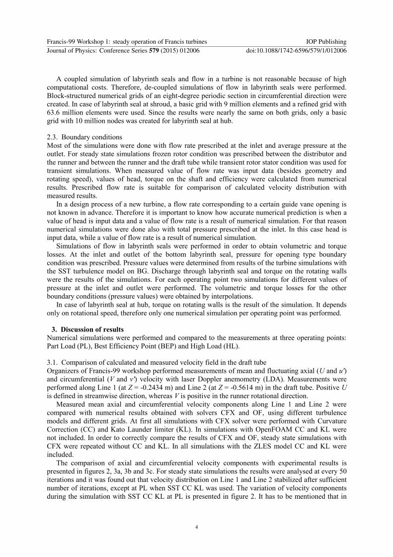
At BEP and HL velocity distribution along Line 1 and Line 2 no longer depends only on turbulence
model, different results were obtained also due to different grid and different solver. All simulations
predicted too small axial velocity in the middle of the draft tube (at r = 0). The region of disagreement
in the middle of the draft tube is wider when OF solver was used. Circumferential velocity component
at the BEP and at the HL is most accurately predicted by the ZLES model. All other models predicted
too large circumferential velocity in opposite direction of runner rotation at the region in the middle of
the draft tube.
It is difficult to conclude which turbulence model provided the best results. For example, at PL, the
axial velocity component obtained with k-ε model agrees well with measurement near the wall but the
agreement is much worse in the middle of the draft tube. On the contrary, SST and ZLES predicted
much too large axial velocity component near the wall but they are more successful in the middle of
the draft tube. For circumferential velocity component on Line 1 the best agreement was obtained with
k-ε CC KL and with SST, while on Line 2 the best agreement was obtained with k-ε.
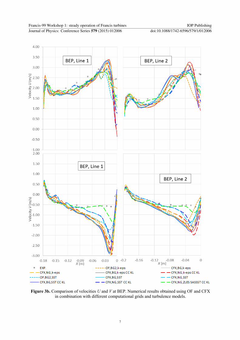
Velocity fluctuations are presented in figure 4a and 4b. Fluctuating velocities predicted with ZLES
agree with the experimental results well. Larger disagreement was obtained only at PL for v'.
Figure 2. Velocities U and V during steady state simulations with SST CC KL at PL.
Francis-99 Workshop 1: steady operation of Francis turbines IOP PublishingJournal of Physics: Conference Series 579 (2015) 012006 doi:10.1088/1742-6596/579/1/012006
5
Figure 3a. Comparison of velocities U and V at PL. Numerical results obtained using OF and CFX in
combination with different computational grids and turbulence models.
Francis-99 Workshop 1: steady operation of Francis turbines IOP PublishingJournal of Physics: Conference Series 579 (2015) 012006 doi:10.1088/1742-6596/579/1/012006
6
Figure 3b. Comparison of velocities U and V at BEP. Numerical results obtained using OF and CFX
in combination with different computational grids and turbulence models.
Francis-99 Workshop 1: steady operation of Francis turbines IOP PublishingJournal of Physics: Conference Series 579 (2015) 012006 doi:10.1088/1742-6596/579/1/012006
7
Figure 3c. Comparison of velocities U and V at HL. Numerical results obtained using OF and CFX in
combination with different computational grids and turbulence models.
Francis-99 Workshop 1: steady operation of Francis turbines IOP PublishingJournal of Physics: Conference Series 579 (2015) 012006 doi:10.1088/1742-6596/579/1/012006
8
Figure 4a. Fluctuating axial velocity at Line 1 and Line 2. Comparison of experimental and CFX
results on NG obtained with ZLES model.
Figure 4b. Fluctuating circumferential velocity at Line 1 and Line 2. Comparison of experimental and
CFX results on NG obtained with ZLES model.
Francis-99 Workshop 1: steady operation of Francis turbines IOP PublishingJournal of Physics: Conference Series 579 (2015) 012006 doi:10.1088/1742-6596/579/1/012006
9
PL BEP HL
U exp.
U ZLES
V exp.
V ZLES
Figure 5. Axial (U) and circumferential (V) velocities at Plane 1, comparison of experimental and
CFX results on NG with ZLES model.
Francis-99 Workshop 1: steady operation of Francis turbines IOP PublishingJournal of Physics: Conference Series 579 (2015) 012006 doi:10.1088/1742-6596/579/1/012006
10
U exp.
U ZLES
V exp.
V ZLES
Figure 6. Axial (U) and circumferential (V) velocities at Plane 2, comparison of experimental and
CFX results on NG with ZLES model.
Instantaneous velocity values of ZLES NG on Plane 1 and 2 are compared to phase-resolved values
of experimental data on corresponding Line 1 and Line 2 (figures 5 and 6). Phase-resolved
Francis-99 Workshop 1: steady operation of Francis turbines IOP PublishingJournal of Physics: Conference Series 579 (2015) 012006 doi:10.1088/1742-6596/579/1/012006
11
experimental data was averaged over many runner rotations. Such post-processing can capture wakes
behind runner blades, whereas all other phenomena in the draft tube are circumferentially averaged.
From such standpoint it can be concluded that ZLES NG simulation predicts range of velocity field in
draft tube well (figures 5 and 6). Wakes behind runner blades on Plane 1 are in comparison with the
experiment less visible.
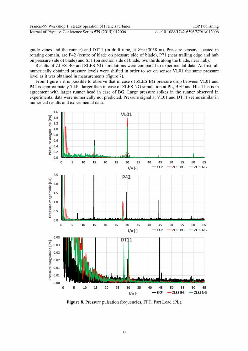
3.2. Pressure pulsation
The organizers of Turbine-99 workshop performed time-dependent pressure measurements. Pressure
sensors, located in stationary frames and presented in this paper are VL01 (in vaneless space between
Figure 7. Pressure pulsation at five locations at Part Load (PL), BEP and High Load (HL).
Francis-99 Workshop 1: steady operation of Francis turbines IOP PublishingJournal of Physics: Conference Series 579 (2015) 012006 doi:10.1088/1742-6596/579/1/012006
12
guide vanes and the runner) and DT11 (in draft tube, at Z=-0.3058 m). Pressure sensors, located in
rotating domain, are P42 (centre of blade on pressure side of blade), P71 (near trailing edge and hub
on pressure side of blade) and S51 (on suction side of blade, two thirds along the blade, near hub).
Results of ZLES BG and ZLES NG simulations were compared to experimental data. At first, all
numerically obtained pressure levels were shifted in order to set on sensor VL01 the same pressure
level as it was obtained in measurements (figure 7).
From figure 7 it is possible to observe that in case of ZLES BG pressure drop between VL01 and
P42 is approximately 7 kPa larger than in case of ZLES NG simulation at PL, BEP and HL. This is in
agreement with larger runner head in case of BG. Large pressure spikes in the runner observed in
experimental data were numerically not predicted. Pressure signal at VL01 and DT11 seems similar in
numerical results and experimental data.
Figure 8. Pressure pulsation frequencies, FFT, Part Load (PL).
Francis-99 Workshop 1: steady operation of Francis turbines IOP PublishingJournal of Physics: Conference Series 579 (2015) 012006 doi:10.1088/1742-6596/579/1/012006
13
Fourier analysis of pressure signals at PL was carried out in figure 8. Two sources of peaks can be
observed in charts. The first source of peaks is guide vane cascade with 28 blades, at 189.56 Hz
(189.56 s-1 / 6.77 s-1 = 28). The peak can be observed in runner (e.g., P42) and in draft tube (DT11).
The second source is runner with 30 blades, with peak at 203.1 Hz (203.1 s-1 / 6.77 s-1 = 30). It can be
observed at VL01 and at DT11. There is also a peak at half of the latter frequency (at 101.55 Hz),
probably because of the differences between 15 splitter and 15 full-length blades. There are also some
peaks at multiplicators of 101.55 Hz (e.g., in VL01). All of these peaks were predicted by ZLES BG
and ZLES NG simulations.
Some of the peaks in figure 8 were not predicted by numerical simulations. For instance, at P42
there are peaks with large magnitude, resembling pressure peaks due to runner blades in VL01.
However, the analysis reveals that their frequency is somewhat lower. For instance, a pressure peak in
P42 and in DT11 is present at 200.06 Hz instead of at 203.1 Hz.
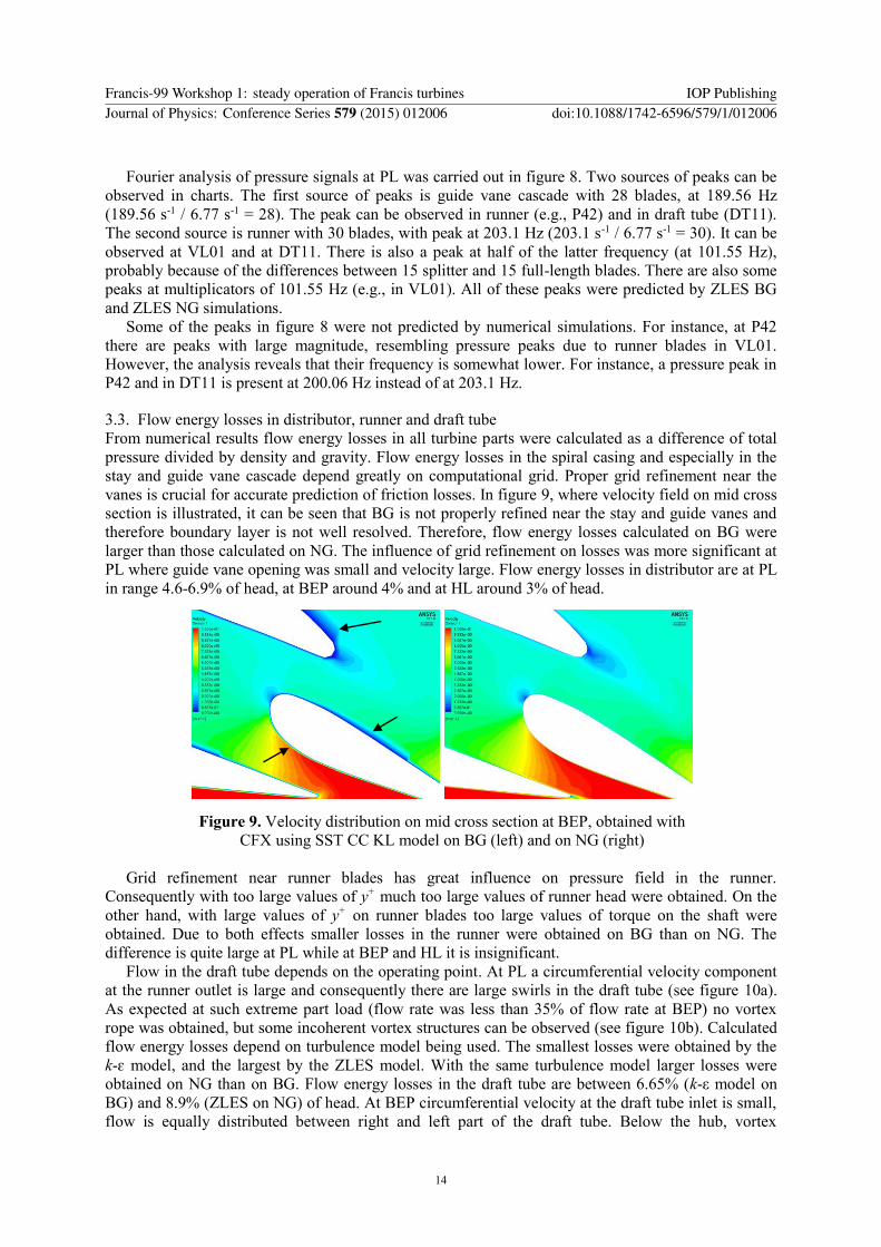
3.3. Flow energy losses in distributor, runner and draft tube
From numerical results flow energy losses in all turbine parts were calculated as a difference of total
pressure divided by density and gravity. Flow energy losses in the spiral casing and especially in the
stay and guide vane cascade depend greatly on computational grid. Proper grid refinement near the
vanes is crucial for accurate prediction of friction losses. In figure 9, where velocity field on mid cross
section is illustrated, it can be seen that BG is not properly refined near the stay and guide vanes and
therefore boundary layer is not well resolved. Therefore, flow energy losses calculated on BG were
larger than those calculated on NG. The influence of grid refinement on losses was more significant at
PL where guide vane opening was small and velocity large. Flow energy losses in distributor are at PL
in range 4.6-6.9% of head, at BEP around 4% and at HL around 3% of head.
Figure 9. Velocity distribution on mid cross section at BEP, obtained with
CFX using SST CC KL model on BG (left) and on NG (right)
Grid refinement near runner blades has great influence on pressure field in the runner.
Consequently with too large values of y+ much too large values of runner head were obtained. On the
other hand, with large values of y+ on runner blades too large values of torque on the shaft were
obtained. Due to both effects smaller losses in the runner were obtained on BG than on NG. The
difference is quite large at PL while at BEP and HL it is insignificant.
Flow in the draft tube depends on the operating point. At PL a circumferential velocity component
at the runner outlet is large and consequently there are large swirls in the draft tube (see figure 10a).
As expected at such extreme part load (flow rate was less than 35% of flow rate at BEP) no vortex
rope was obtained, but some incoherent vortex structures can be observed (see figure 10b). Calculated
flow energy losses depend on turbulence model being used. The smallest losses were obtained by the
k-ɛ model, and the largest by the ZLES model. With the same turbulence model larger losses were
obtained on NG than on BG. Flow energy losses in the draft tube are between 6.65% (k-ε model on
BG) and 8.9% (ZLES on NG) of head. At BEP circumferential velocity at the draft tube inlet is small,
flow is equally distributed between right and left part of the draft tube. Below the hub, vortex
Francis-99 Workshop 1: steady operation of Francis turbines IOP PublishingJournal of Physics: Conference Series 579 (2015) 012006 doi:10.1088/1742-6596/579/1/012006
14
structures are rolled around strong vertical central vortex. Flow energy losses are between 0.46 - 0.6%
of head, depending on turbulence model and grid. At HL, flow in the draft tube looks very similar as at
BEP. Also vortex structures are similar. Flow energy losses are between 0.56 - 0.65% of head.
Figure 10. Flow in the draft tube at Part Load (bottom), BEP (middle) and High Load (top):
a) streamlines; b) vortex structures. Results of CFX on NG with the ZLES turbulence model.
3.4. Labyrinth seals
The results of flow simulation in the bottom labyrinth seal are volumetric losses and torque losses.
They depend on rotational speed of the runner and also on pressure difference between labyrinth seal
inlet (before the runner) and outlet (behind the runner). These values of pressure were obtained from
the results of flow simulations in the turbine and differed due to used turbulence model and grid.
Volumetric losses are approximately the same for all three operating points, but they are, due to small
flow rate, more important at PL than at the other two operating points. Torque losses are the largest at
PL mainly due to the highest rotational speed. Torque losses in the top labyrinth seal depend only on
runner rotating speed and therefore they are the largest at PL and the smallest at the BEP. The results
for the bottom and the top labyrinth seals at all three operating points are presented in table 3.
Table 3. Volumetric and torque losses in labyrinth seals. Operating
point
Rotating
Speed
(s-1)
Volumetric losses in
bottom labyrinth seal
(l/s)
Torque losses in bottom
labyrinth seal
(Nm)
Torque losses in top
labyrinth seal
(Nm)
PL 6.77 0.435 8.86 7.335
BEP 5.59 0.426 6.10 5.355
HL 6.16 0.47 7.40 6.3
The sum of torque losses in bottom and top labyrinth seals were subtracted from the torque on the
shaft calculated from the results of flow simulations in the turbine. In such a way corrected torque
better agreed with the measurements.
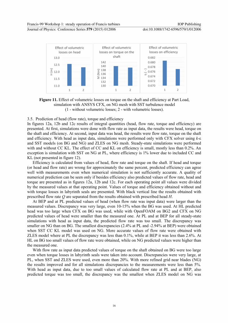
Relative values of volumetric losses (volumetric losses divided by the discharge value) are the
largest at PL, therefore at this operating point a flow simulation in the turbine was performed with
prescribed mass sink before the runner and mass source behind the runner. This simulation was
performed only with CFX on slightly modified NG mesh with SST CC KL turbulence model. Due to
smaller discharge in the runner, calculated head and torque on the shaft slightly decreased. Due to
volumetric losses also the efficiency value decreased. The effect of volumetric losses on results is
presented in figure 11. It can be expected that for the other operating points the effect of volumetric
losses would be even smaller.
Francis-99 Workshop 1: steady operation of Francis turbines IOP PublishingJournal of Physics: Conference Series 579 (2015) 012006 doi:10.1088/1742-6596/579/1/012006
15
Figure 11. Effect of volumetric losses on torque on the shaft and efficiency at Part Load,
simulation with ANSYS CFX, on NG mesh with SST turbulence model
(1 - without volumetric losses; 2 - with volumetric losses).
3.5. Prediction of head (flow rate), torque and efficiency
In figures 12a, 12b and 12c results of integral quantities (head, flow rate, torque and efficiency) are
presented. At first, simulations were done with flow rate as input data, the results were head, torque on
the shaft and efficiency. At second, input data was head, the results were flow rate, torque on the shaft
and efficiency. With head as input data, simulations were performed only with CFX solver using k-ε
and SST models (on BG and NG) and ZLES on NG mesh. Steady-state simulations were performed
with and without CC KL. The effect of CC and KL on efficiency is small, mostly less than 0.2%. An
exception is simulation with SST on NG at PL, where efficiency is 1% lower due to included CC and
KL (not presented in figure 12).
Efficiency is calculated from values of head, flow rate and torque on the shaft. If head and torque
(or head and flow rate) are wrong for approximately the same percent, predicted efficiency can agree
well with measurements even when numerical simulation is not sufficiently accurate. A quality of
numerical prediction can be seen only if besides efficiency also predicted values of flow rate, head and
torque are presented as in figures 12a, 12b and 12c. For each operating point all values were divided
by the measured values at that operating point. Values of torque and efficiency obtained without and
with torque losses in labyrinth seals are presented. With black vertical line the results obtained with
prescribed flow rate Q are separated from the results obtained with prescribed head H.
At BEP and at PL predicted values of head (when flow rate was input data) were larger than the
measured values. Discrepancy was very large, even 10-15% when the BG was used. At HL predicted
head was too large when CFX on BG was used, while with OpenFOAM on BG2 and CFX on NG
predicted values of head were smaller than the measured one. At PL and at BEP for all steady-state
simulations with head as input data, the predicted flow rate was too small. The discrepancy was
smaller on NG than on BG. The smallest discrepancies (2.4% at PL and -2.94% at BEP) were obtained
when SST CC KL model was used on NG. More accurate values of flow rate were obtained with
ZLES model where at PL the discrepancy was less than 0.1%, while at BEP it was less than 2.6%. At
HL on BG too small values of flow rate were obtained, while on NG predicted values were higher than
the measured one.
With flow rate as input data predicted values of torque on the shaft obtained on BG were too large
even when torque losses in labyrinth seals were taken into account. Discrepancies were very large, at
PL, when SST and ZLES were used, even more than 20%. With more refined grid near blades (NG)
the results improved and for all simulations discrepancies to the measurements were less than 5%.
With head as input data, due to too small values of calculated flow rate at PL and at BEP, also
predicted torque was too small, the discrepancy was the smallest when ZLES model on NG was
Francis-99 Workshop 1: steady operation of Francis turbines IOP PublishingJournal of Physics: Conference Series 579 (2015) 012006 doi:10.1088/1742-6596/579/1/012006
16
Figure 12a. Comparison of numerical results to the experimental values, Part Load.
CFX simulations were performed with CC and KL.
Figure 12b. Comparison of numerical results to the experimental values, BEP.
CFX simulations were performed with CC and KL.
Francis-99 Workshop 1: steady operation of Francis turbines IOP PublishingJournal of Physics: Conference Series 579 (2015) 012006 doi:10.1088/1742-6596/579/1/012006
17
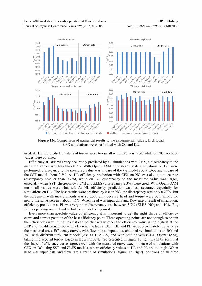
Figure 12c. Comparison of numerical results to the experimental values, High Load.
CFX simulations were performed with CC and KL.
used. At HL the predicted values of torque were too small when BG was used, while on NG too large
values were obtained.
Efficiency at BEP was very accurately predicted by all simulations with CFX, a discrepancy to the
measured values was less than 0.7%. With OpenFOAM only steady state simulations on BG were
performed, discrepancy to the measured value was in case of the k-ε model about 1.6% and in case of
the SST model about 2.3%. At HL efficiency prediction with CFX on NG was also quite accurate
(discrepancy smaller than 0.7%), while on BG discrepancy to the measured value was larger,
especially when SST (discrepancy 1.5%) and ZLES (discrepancy 2.3%) were used. With OpenFOAM
too small values were obtained. At HL efficiency prediction was less accurate, especially for
simulations on BG. The best results were obtained by k-ε on NG, the discrepancy was only 0.27%. But
the agreement with measurements was so good only because head and torque were both wrong for
nearly the same percent, about 4.6%. When head was input data and flow rate a result of simulation,
efficiency prediction at PL was very poor, discrepancy was between 3.7% (ZLES, NG) and -10% (k-ε,
BG), depending on grid and turbulence model being used.
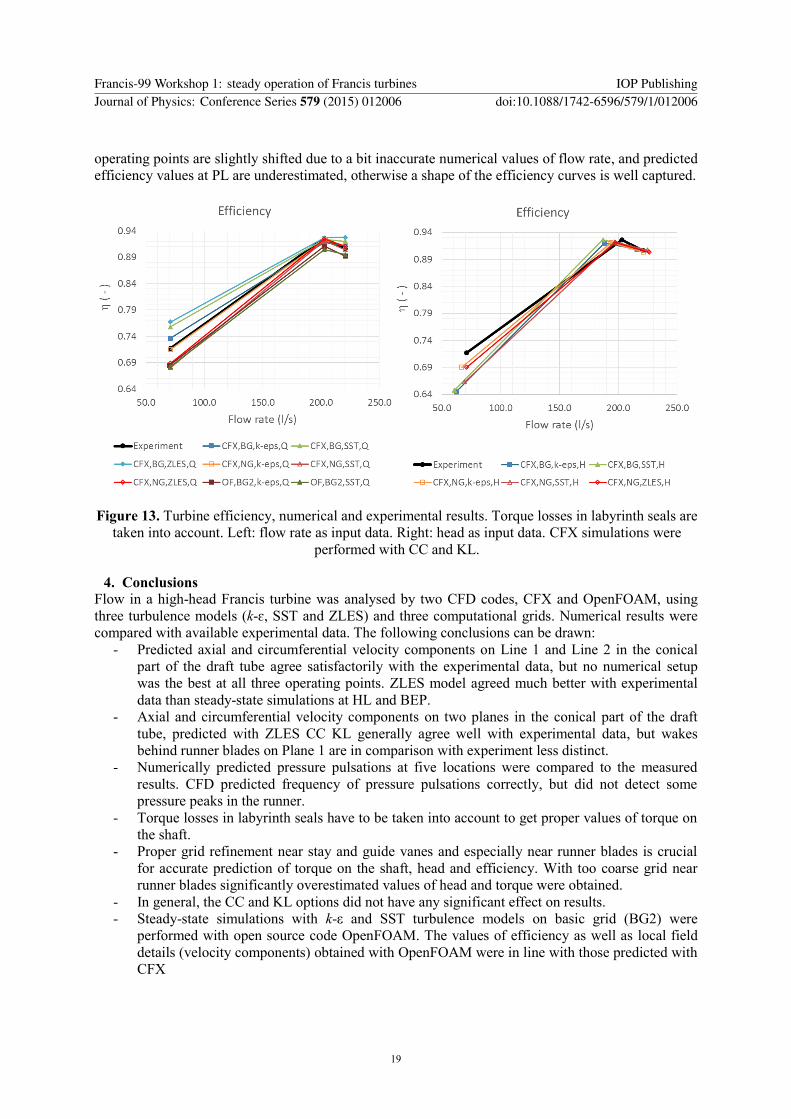
Even more than absolute value of efficiency it is important to get the right shape of efficiency
curve and correct position of the best efficiency point. Three operating points are not enough to obtain
the efficiency curve, but at least it can be checked whether the efficiency value is the highest at the
BEP and the differences between efficiency values at BEP, HL and PL are approximately the same as
the measured ones. Efficiency curves, with flow rate as input data, obtained by simulations on BG and
NG, with different turbulent models (k-ε, SST, ZLES) and with both solvers (CFX, OpenFOAM),
taking into account torque losses in labyrinth seals, are presented in figure 13, left. It can be seen that
the shape of efficiency curves agrees well with the measured curve except in case of simulations with
CFX on BG using SST and ZLES models, where efficiency values at HL and PL are too high. When
head was input data and flow rate a result of simulations (figure 13, right), positions of all three
Francis-99 Workshop 1: steady operation of Francis turbines IOP PublishingJournal of Physics: Conference Series 579 (2015) 012006 doi:10.1088/1742-6596/579/1/012006
18
operating points are slightly shifted due to a bit inaccurate numerical values of flow rate, and predicted
efficiency values at PL are underestimated, otherwise a shape of the efficiency curves is well captured.
Figure 13. Turbine efficiency, numerical and experimental results. Torque losses in labyrinth seals are
taken into account. Left: flow rate as input data. Right: head as input data. CFX simulations were
performed with CC and KL.
4. Conclusions
Flow in a high-head Francis turbine was analysed by two CFD codes, CFX and OpenFOAM, using
three turbulence models (k-ɛ, SST and ZLES) and three computational grids. Numerical results were
compared with available experimental data. The following conclusions can be drawn:
- Predicted axial and circumferential velocity components on Line 1 and Line 2 in the conical
part of the draft tube agree satisfactorily with the experimental data, but no numerical setup
was the best at all three operating points. ZLES model agreed much better with experimental
data than steady-state simulations at HL and BEP.
- Axial and circumferential velocity components on two planes in the conical part of the draft
tube, predicted with ZLES CC KL generally agree well with experimental data, but wakes
behind runner blades on Plane 1 are in comparison with experiment less distinct.
- Numerically predicted pressure pulsations at five locations were compared to the measured
results. CFD predicted frequency of pressure pulsations correctly, but did not detect some
pressure peaks in the runner.
- Torque losses in labyrinth seals have to be taken into account to get proper values of torque on
the shaft.
- Proper grid refinement near stay and guide vanes and especially near runner blades is crucial
for accurate prediction of torque on the shaft, head and efficiency. With too coarse grid near
runner blades significantly overestimated values of head and torque were obtained.
- In general, the CC and KL options did not have any significant effect on results.
- Steady-state simulations with k-ε and SST turbulence models on basic grid (BG2) were
performed with open source code OpenFOAM. The values of efficiency as well as local field
details (velocity components) obtained with OpenFOAM were in line with those predicted with
CFX
Francis-99 Workshop 1: steady operation of Francis turbines IOP PublishingJournal of Physics: Conference Series 579 (2015) 012006 doi:10.1088/1742-6596/579/1/012006
19
Acknowledgments
The research was partly funded by the European Commission - FP7-PEOPLE-2013-IAPP - Grant No.
612279 and by the Slovenian Research Agency ARRS - Contract No. 1000-09-160263.
References
[1] Jošt D, Lipej A, Mežnar P 2008 Numerical prediction of efficiency, cavitation and unsteady
phenomena in water Turbines, 9th Biennial ASME Conf. on Eng. Sys. Design and Analysis,
ESDA08 (Haifa, Israel)
[2] Chirag T, Cervantes M J, Gandhi B K and Dahlhaug O G 2013 Experimental and numerical
studies for a high head Francis turbine at several operating points J. Fluids Eng. 135 111102
[3] Menter F R, Kuntz M and Langtry R 2003 Ten years of industrial experience with the SST
turbulence model Turbulence, Heat and Mass Transfer 4 eds. K Hanjalić, Y Nagano and M
Tummers (New York: Begell House) pp 625–632
[4] Menter F R and Esch T 2001 Elements of industrial heat transfer prediction 16th Brazilian
Congr. of Mech. Eng. (Uberlandia, Brazil)
[5] Jošt D, Škerlavaj A, Lipej A 2012 Numerical flow simulation and efficiency prediction for axial
turbines by advanced turbulence models IOP Conf. Ser.: Earth Environ. Sci. 15(6) p 062016
[6] Jošt D, Škerlavaj A, Lipej A 2014 Improvement of efficiency prediction for a Kaplan turbine
with advanced turbulence models J. Mech. Eng. 60(2) pp 124–34
[7] Menter F R, Gabaruk A, Smirnov P, Cokljat D and Mathey F 2010 Scale-adaptive simulation
with artificial forcing Progress in Hybrid RANS-LES Modelling ed. S-H Peng, P Doerffer
and W Haase (Berlin: Springer) pp 235–46
[8] Adamian D and Travin A 2011 An efficient generator of synthetic turbulence at RANS–LES
interface in embedded LES of wall-bounded and free shear flows Computational Fluid
Dynamics 2010 ed. A Kuzmin (Berlin: Springer) 739–44
[9] Egorov Y and Menter F 2008 Development and application of SST-SAS turbulence model in
the DESIDER project Advances in Hybrid RANS-LES Modelling ed. S-H Peng and W Haase
(Heidelberg: Springer) pp 261–70
[10] Smirnov P E and Menter F 2009 Sensitization of the SST turbulence model to rotation and
curvature by applying the Spalart-Shur correction term J. Turbomach. 131(4) 041010
[11] Kato M and Launder B E 1993 The modelling of turbulent flow around stationary and vibrating
square cylinders Proc. 9th Symp. on Turbulent Shear Flows pp 10.4.1–10.4.6.
[12] Shur M L, Spalart P R, Strelets M K and Travin A K 2008 A hybrid RANS-LES approach with
delayed-DES and wall-modeled LES capabilities Int. J. Heat Fluid Flow 29(6) pp 1638–49
Francis-99 Workshop 1: steady operation of Francis turbines IOP PublishingJournal of Physics: Conference Series 579 (2015) 012006 doi:10.1088/1742-6596/579/1/012006