J. Fluid Mech. (2007), vol. 591, pp. 215–253. c 2007 Cambridge University Press doi:10.1017/S0022112007008129 Printed in the United Kingdom 215 Numerical simulation of the compressible mixing layer past an axisymmetric trailing edge FRANCK SIMON 1 , SEBASTIEN DECK 1 , PHILIPPE GUILLEN 1 , PIERRE SAGAUT 2 AND ALAIN MERLEN 3 1 ONERA, Applied Aerodynamics Department, F-92322 Chˆ atillon, France 2 Institut Jean Le Rond d’Alembert, UMR 7190, Universit´ e Pierre et Marie Curie - Paris 6, F-75005 Paris, France 3 Laboratoire de M´ ecanique de Lille, UMR 8107, Universit´ e des sciences et technologies de Lille, F-59655 Villeneuve d’Ascq, France (Received 23 August 2006 and in revised form 25 June 2007) Numerical simulation of a compressible mixing layer past an axisymmetric trailing edge is carried out for a Reynolds number based on the diameter of the trailing edge approximately equal to 2.9 × 10 6 . The free-stream Mach number at separation is equal to 2.46, which corresponds to experiments and leads to high levels of compressibility. The present work focuses on the evolution of the turbulence field through extra strain rates and on the unsteady features of the annular shear layer. Both time- averaged and instantaneous data are used to obtain further insight into the dynamics of the flow. An investigation of the time-averaged flow field reveals an important shear-layer growth rate in its initial stage and a strong anisotropy of the turbulent field. The convection velocity of the vortices is found to be somewhat higher than the estimated isentropic value. This corroborates findings on the domination of the supersonic mode in planar supersonic/subsonic mixing layers. The development of the shear layer leads to a rapid decrease of the anisotropy until the onset of streamline realignment with the axis. Due to the increase of the axisymmetric constraints, an adverse pressure gradient originates from the change in streamline curvature. This recompression is found to slow down the eddy convection. The foot shock pattern features several convected shocks emanating from the upper side of the vortices, which merge into a recompression shock in the free stream. Then, the flow accelerates and the compressibility levels quickly drop in the turbulent developing wake. Some evidence of the existence of large-scale structures in the near wake is found through the domination of the azimuthal mode m = 1 for a Strouhal number based on trailing- edge diameter equal to 0.26. 1. Introduction The understanding of free shear flows is of primary interest as they include numerous fundamental but also complex physics features and have been the focus of many studies for decades. As reasonable knowledge of low-speed shear layers was achieved, research interest was pushed toward the supersonic case thus revealing strong differences with subsonic mixing layers. The major discrepancies appear to be a reduction in the shear layer growth rate coupled with a decrease of the turbulent Reynolds stresses magnitude. Such behaviour has been found to be a direct effect of
doi:10.1017/S0022112007008129 Printed in the United Kingdom
215
Numerical simulation of the compressible mixinglayer past an axisymmetric trailing edge
FRANCK SIMON1, SEBASTIEN DECK1,PHILIPPE GUILLEN1, P IERRE SAGAUT 2
AND ALAIN MERLEN 3
1ONERA, Applied Aerodynamics Department, F-92322 Chatillon, France2Institut Jean Le Rond d’Alembert, UMR 7190, Universite Pierre et Marie Curie - Paris 6,
F-75005 Paris, France3Laboratoire de Mecanique de Lille, UMR 8107, Universite des sciences et technologies de Lille,
F-59655 Villeneuve d’Ascq, France
(Received 23 August 2006 and in revised form 25 June 2007)
Numerical simulation of a compressible mixing layer past an axisymmetric trailingedge is carried out for a Reynolds number based on the diameter of the trailing edgeapproximately equal to 2.9×10⁶. The free-stream Mach number at separation is equalto 2.46, which corresponds to experiments and leads to high levels of compressibility.The present work focuses on the evolution of the turbulence field through extrastrain rates and on the unsteady features of the annular shear layer. Both time-averaged and instantaneous data are used to obtain further insight into the dynamicsof the flow. An investigation of the time-averaged flow field reveals an importantshear-layer growth rate in its initial stage and a strong anisotropy of the turbulentfield. The convection velocity of the vortices is found to be somewhat higher thanthe estimated isentropic value. This corroborates findings on the domination of thesupersonic mode in planar supersonic/subsonic mixing layers. The development ofthe shear layer leads to a rapid decrease of the anisotropy until the onset of streamlinerealignment with the axis. Due to the increase of the axisymmetric constraints, anadverse pressure gradient originates from the change in streamline curvature. Thisrecompression is found to slow down the eddy convection. The foot shock patternfeatures several convected shocks emanating from the upper side of the vortices,which merge into a recompression shock in the free stream. Then, the flow acceleratesand the compressibility levels quickly drop in the turbulent developing wake. Someevidence of the existence of large-scale structures in the near wake is found throughthe domination of the azimuthal mode m =1 for a Strouhal number based on trailing-edge diameter equal to 0.26.
1. IntroductionThe understanding of free shear flows is of primary interest as they include
numerous fundamental but also complex physics features and have been the focusof many studies for decades. As reasonable knowledge of low-speed shear layerswas achieved, research interest was pushed toward the supersonic case thus revealingstrong differences with subsonic mixing layers. The major discrepancies appear to bea reduction in the shear layer growth rate coupled with a decrease of the turbulentReynolds stresses magnitude. Such behaviour has been found to be a direct effect of
216 F. Simon, S. Deck, P. Guillen, P. Sagaut and A. Merlen
the compressibility and the scaling parameter was found to be the convective Machnumber Mc (Bogdanoff 1983; Papamoschou & Roshko 1988). Mc was derived fromisentropic assumptions and is
Mc =U1 − U2
a1 + a2
(1.1)
where the subscripts 1 and 2 respectively describe the high- and the low-speedstreams. An early interpretation of this stabilizing effect involved a reduction ofcommunication in the shear layer by Papamoschou (1990) and Breidenthal (1990).First observed in experiments (Papamoschou & Roshko 1988; Papamoschou 1991;Gruber, Messersmith & Dutton 1993; Barre, Quine & Dussauge 1994; Clemens &Mungal 1995) it also has been highlighted by means of direct numerical simulations(DNS) (Sandham & Reynolds 1989; 1991; Sarkar 1995 Vreman, Sandham & Luo 1996Freund, Lele & Moin 2000; Pantano & Sarkar 2002). It has been demonstrated thatthe normalized pressure–strain term decreases with increasing Mc. The consequenceof this compressibility effect is an energy transfer reduction from the streamwiseto cross-stream velocity fluctuations involving a decay of the turbulence productionterm in the Reynolds stresses transport equation. From a theoretical point of view,such an influence on homogeneous sheared turbulence has also been demonstratedby Simone, Coleman & Cambon (1997) using linear rapid-distortion theory. The useof linear stability analysis of compressible mixing layers gives the same conclusions(Jackson & Grosch 1989; Sandham & Reynolds 1991).
It has been demonstrated that increasing Mc leads to a physical change in thegeometry of the large-scale structures. For Mc values less than 0.6, the instabilityprocess is bi-dimensional with large spanwise correlated structures originating fromthe Kelvin–Helmholtz (KH) instability. These spanwise rollers are quite easy tofollow in the flow field and phenomena such as pairing or merging can also clearlybe observed participating in the shear layer growth. For values above 0.6, obliquewaves compete with bi-dimensional instability modes. Finally, when Mc > 1, theinstability waves are three-dimensional and the growth rate of the most amplifiedmode is greatly reduced compared to the bi-dimensional mode in low-Mc cases.This shift in the instability process comes with a modification of the coherent-structure shape in supersonic mixing layers. Moreover, these structures are difficultto identify and to track due to their less coherent properties. Pairing and mergingprocesses, seem to be inhibited, at least in the initial stage of development of the freecompressible shear layer. Sandham & Reynolds (1991) observed λ-vortices staggeredin the streamwise direction at high Mc values. Another important finding of thelinear stability studies is the departure from the isentropic Mc model under highlycompressible conditions. Jackson & Grosch (1989) have highlighted the existence ofa slow mode and a supersonic mode at high Mc in addition to the neutral mode (alsocalled the central mode) already existing in the subsonic case. This explains someexperimental observations of asymmetric behaviour of supersonic mixing layers. Inthe two-stream supersonic–supersonic case, the slow mode develops whereas in thesupersonic–subsonic case, the fast mode dominates.
In the case of axisymmetric supersonic shear layers, previous studies (Fourguette,Mungal & Dibble 1991; Freund et al. 2000; Thurow, Ssamimy & Lempert 2003) havedemonstrated the three-dimensional shape of the turbulent eddies, as in the planarcase. Freund (2000) have performed direct simulations of temporally developing roundcompressible jets in the early stages of their development. They observed a diminutionof the velocity fluctuations with the convective Mach number. This behaviour, similar
Compressible mixing layer past an axisymmetric trailing edge 217
to that encountered in planar shear layers, is somewhat reduced in the axisymmetriccase. However, the authors could not state if it was a direct effect of the geometryconfiguration or due to greater turbulence intensity in the non-similar states of the jet.Moreover, in their more compressible case (Mc = 0.87), Thurow et al. (2003) observeda bimodal instability with the appearance of both slow and fast modes, which differsfrom planar mixing layer studies.
However, in some specific cases, axisymmetric compressible shear layers can leadto the occurrence of a wide range of phenomena coupled with complex interactions.To investigate such flows, the separation process past a blunt-base axisymmetrictrailing edge is used to generate a supersonic annular shear layer. This particulargeometrical configuration involves an important modification of the whole flow fieldcompared to the canonical case. The separating process transforms the incomingboundary layer into an annular mixing layer. On passing through the expansionfan centred at the base, the developing shear layer is deflected toward the axis andthen grow on moving downstream. On approaching the axis, concave curvature effectsoriginating from the increasing axisymmetrical constraint appear. An adverse pressuregradient then originates from the change in lateral streamline curvature leading tothe formation of a recompression shock in the free stream like that encountered inramp compression configurations (see for example Adams 2000). On passing throughthe pressure gradient, the flow realigns with the axis and the axisymmetric mixinglayer transitions into a turbulent wake. Both the streamline curvature and the adversepressure gradient constitute extra strain rates (as defined by Bradshaw (1974) forsupersonic boundary layers studies) which can deeply alter the turbulence structureof the flow field.
In the past, due to measurement difficulties, attention has been focused on the farwake. For example, Demetriades (1968, 1976) has experimentally studied the far fieldbehind a slender axisymmetric body and found some evidence of the existence oflarge-scale structures (organized structures have also been experimentally found insubsonic axisymmetric wakes by Roberts (1973), Fuchs, Mercker & Michel (1979)and more recently by Depres (2003)). However, excepting the work of Gaviglio et al.(1977), the near wake has been studied only very recently thanks to the improvementof non-intrusive measurement tools. Such a case has been experimentally investigatedat the University of Illinois where this configuration has received particular attentionwith the use of visualizations and laser Doppler velocimetry (LDV). A lot of workhas been done by Dutton and co-workers in postprocessing instantaneous snapshotsto gain insight into the vortex dynamics. However, the experimental nature of theirwork prevent them from directly acquiring unsteady data in the separated flow field,thus limiting our comprehension of such flows. During the last ten years, severalworks have been devoted to the simulation of such a flow in order to improveturbulence model predictions or to validate new hybrid numerical approaches (seefor example, Fureby, Nilsson & Andersson 1999; Forsythe et al. 2002; Baurle et al.2003; Kawai & Fujii 2005). Unfortunately, these numerical studies have focused ontime-averaged results and none of them has been used to assess the unsteadinessof the flow, except the study of Sandberg & Fasel (2006a, b) who investigated thetransitional wake at ReD = 100 000 with D the diameter of the trailing edge, with theuse of DNS and linear stability investigations. A major result is the coexistence ofconvective shear layer instabilities and of an absolute instability of the recirculatingflow.
Numerical simulation is therefore a useful tool to go beyond the shortcomings ofthe available experimental data as some questions remain open:
218 F. Simon, S. Deck, P. Guillen, P. Sagaut and A. Merlen
(i) Does the initial part of the mixing layer behave as in the planar case? What isthe dynamics of the eddies in the developing shear layer?
(ii) How do the extra strain rates alter the turbulent field and the shear layerdynamics?
(iii) The far field is known to be self-similar but what happens in the transitionregion before the wake attains a fully developed state?
(iv) A characteristic feature of such a configuration is the existence of a subsonicrecirculating flow enclosed in the supersonic annular mixing layer. What role doesthis bubble play in the shear layer dynamics and does a forcing through a feedbackmechanism exist?
The present work investigates the unsteadiness of the compressible shear layerdevelopment past an axisymmetric trailing edge and the influence of extra strain rateson the turbulence field by means of numerical simulation. The paper is organized asfollows. First the main features of the experimental setup and the test case will bedescribed. Then, the numerical code and the simulation methodology as well as themesh grid will be described. A mean flow analysis will be performed to investigate theclassical properties of supersonic base flows. In the two following sections, attentionwill be focused on the description of the shear layer behaviour in terms of time-averaged characteristics, coherent-structure dynamics and spectral analysis. Once theshear layer has been investigated, the recompression region, the turbulent wakedevelopment and the recirculation area will be successively considered.
2. Main features of the experimental setupThe supersonic base flow past an axisymmetric trailing edge was experimentally
investigated at the University of Illinois Gas Dynamics Laboratory by Herrin &Dutton (1994a) for a free-stream Mach number M∞ equal to 2.46 and a Reynoldsnumber per metre equal to 52 × 106. The wind tunnel was specially designed foraxisymmetric base flow investigations and is of blowdown-type. Special care wastaken that the axisymmetry of the flow was not altered on the cylinder due to a slightmisalignment of the model. This test case has been chosen as a consequence of thegreat amount of available data to validate the numerical results.
This bluntbase case was investigated using a two-component (LDV) system (Herrin& Dutton (1994a, 1995). Conventional schlieren and shadowgraph photography werealso used to investigate the coherent-structure properties. Planar flow visualizations(both side and end views) using the single-pulse, planar Mie scattering techniquehave also been published by Bourdon & Dutton (1999, 2000) and Cannon, Elliott &Dutton (2005). Mean-static pressure measurements and high-frequency measurementsusing Kulite pressure transducers have been published by Janssen & Dutton (2004).
Also, the planar case (Smith & Dutton 1996; Messersmith & Dutton 1996; Smith& Dutton 1999; 2001) and the boattailed-base case (Herrin & Dutton 1994b, 1995,1997; Bourdon & Dutton 2001) have also received attention, thus providing additionalinsight into the axisymmetric case.
A detailed description of the wind tunnel facility and of the experimental diagnosticscan be found in the above references.
3. Numerical procedure3.1. FLU3M code
The multiblock Navier–Stokes solver used in the present study is the FLU3M codedeveloped by ONERA. The equations are discretized using a second-order- accurate
Compressible mixing layer past an axisymmetric trailing edge 219
upwind finite volume scheme and a cell-centred discretization. The Euler fluxes arediscretized by a modified AUSM+(P) upwind scheme which is fully described in Mary& Sagaut (2002). Time discretization is based on second-order Gear’s formulation aspresented by Pechier et al. (2001). Further details concerning the numerical procedureand the turbulence modelling may be found in Pechier et al. (2001) and Deck et al.(2002). This numerical strategy has already been applied with success to a wide rangeof turbulent flows such as the compressible flow over an open cavity at high Reynoldsnumber (Larcheveque et al. 2003, 2004) and transonic buffet over a supercriticalairfoil (Deck (2005a)).
3.2. Turbulence modelling
Because of the high Reynolds number of the flow, the methodology used in thepresent work is the zonal-detached eddy simulation (ZDES) which is derived fromthe classical detached eddy simulation (called DES97) introduced by Spalart et al.(1997). These methodologies are part of the RANS/LES family (for more details, seethe discussion by Sagaut, Deck & Terracol 2006).
The model was originally based on the Spalart–Allmaras (SA) model which solvesa one-equation turbulence model for the eddy viscosity ν:
Dρν
Dt= cb1Sρν +
1
σ
(∂
∂xj
(µ + ρν)∂ν
∂xj
+ cb2
∂ν
∂xj
ρν
∂xj
)− ρcw1fw
(ν
dw
)2
. (3.1)
The eddy viscosity is defined as:
µt = ρνfv1 = ρνt , fv1 =χ3
χ3 + c3v1
, χ =ν
ν. (3.2)
The fw and fv functions are near-wall correction functions in the finite-Reynolds-number version of the model and we refer to the original papers Spalart & Allmaras(1992, 1994) for details on the constants and the quantities involved. For the currentresearch, the transition terms of the SA model allowing for a shift from a laminar toa turbulent state were turned off.
What is important here is that the model is provided with a destruction term forthe eddy viscosity that contains d , the distance to the closest wall. This term, whenbalanced with the the production term, adjusts the eddy viscosity to scale with thelocal deformation rate S producing an eddy viscosity given by:
ν ∼ Sd2. (3.3)
The idea suggested by Spalart et al. (1997) was to modify the destruction term sothat the RANS model is reduced to an LES subgrid-scale one in the detached flows.They proposed to replace the distance d to the closest wall with d defined by
d = min(d, CDES) (3.4)
where is a characteristic mesh length. Away from the wall, if the destruction termbalances the production one, the eddy viscosity scales with the length and the localvorticity modulus S: νt ∼ S2, then takes the form of Smagorinsky’s SGS-viscosityνSGS ∼
√2SijSij
2, where Sij are the components of the strain tensor. Moreover, thesubgrid model behaves somewhat like a dynamic model because of the materialderivative and the diffusion term. Shur et al. (1999) have calibrated the CDES value byperforming homogeneous isotropic turbulence simulations using high-order schemesand found a value of 0.65. The use of lower-order spatial schemes suggests lowering
220 F. Simon, S. Deck, P. Guillen, P. Sagaut and A. Merlen
this value. In accordance with the previous statement and in agreement with previouswork (Simon et al. (2006)), the CDES constant was set to 0.55 in the present study.
Originally, we chose to define as the largest of the spacings in all three directions
= max = max(x, y, z) (3.5)
so that the model ‘naturally’ switches from the RANS behaviour in the grid regiontypical of a boundary layer, i.e. d = max(x, z) ( y being normal to the wall)to the LES behaviour away from the wall, i.e. d . Nevertheless, and from thebeginning, a special care was given to the region, named the ‘grey area’, where themodel switches, and where the velocity fluctuations (the ‘LES content’), are expectedto be not sufficiently developed to compensate for the loss of modelled turbulentstresses. This can lead to unphysical outcomes, such as an under-estimation of theskin friction, and so motivated, first, the publication of a paper (Spalart 2001) tospecify the character of DES97 meshes, and then, a modification of d , presented as adelayed-DES (Spalart et al. 2006), to extend the RANS mode and prevent ‘modelled-stress depletion’. In order to remove this drawback, Deck (2005a, b) proposed a zonalapproach of the original DES, called zonal-DES or ZDES, in which RANS and DESdomains are selected individually. In RANS regions, the model is forced to behaveas a RANS model, while in DES regions, the model can switch from the RANSmode to the LES mode by means of (3.4). The zonal approach is well-adapted totreat free shear flows, as the user can focus grid refinements on the regions of interestwithout corrupting the boundary-layer properties farther upstream or downstream.For instance, in DES regions, the grid is designed to obtain nearly cubic cells. In theseregions, Deck also suggested adopting the classical characteristic length scale used inLES and based on the cell volume:
= vol = (xyz)1/3. (3.6)
In addition, the near-wall functions of the RANS model are explicitly disabled in theLES mode of DES regions (but not in the RANS mode) as follows (Breuer, Jovicic& Mazaev 2003):
fv1 = 1, fv2 = 0, fw = 1. (3.7)
This choice avoids the low eddy viscosity levels typical of resolved LES regions beingtreated as in boundary layers. The use of (3.6) and (3.7) in DES regions justifiesits notation being different from DES97. In practice, DES switches very quickly tothe LES mode thanks to (3.6) and (3.7). In this way, the LES mode is managed bythe transport equation of νt calibrated for free shear flows plus a destruction termrescaling the subgrid-scale viscosity as a function of the mesh resolution. To completethe closure of the RANS/SGS stress tensor, its deviatoric part τ d is linearly linkedto the deviatoric part of the resolved strain tensor:
τ dij = 2ρνt (Sij − 1
3Sllδij ) (3.8)
while its isotropic part, whose trace equals 2/3 times the specific kinetic energy (ofthe whole of the turbulence in RANS mode or under the gridscale in LES mode),can be included in the pressure term and is often neglected with respect to it. In thepresent work, the subgrid kinetic energy is neglected in the total energy equation.This hypothesis is based on the work by Erlebacher et al. (1992) who demonstratethat it is reasonable to neglect this term without compromising the flow physicsprediction in the case of turbulent Mach numbers Mt lower than 0.60. In the nearwake, the turbulent activity leads to Mt levels up to 0.40 when the resolved turbulent
Compressible mixing layer past an axisymmetric trailing edge 221
8R
10R
8.3R
xz
y
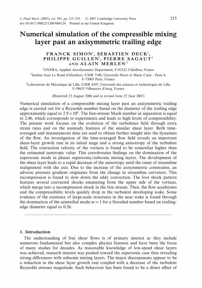
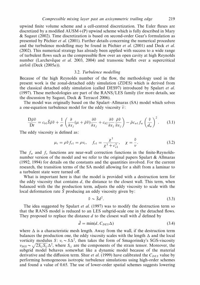
Figure 1. The computational mesh.
kinetic energy is considered (see figure 19). As at the same time, the SGS contributionis very weak, this justifies the use of the present numerical model without alteringsignificantly the resolved flow physics.
It has successfully been used to calculate the transonic buffet phenomenon overa supercritical airfoil (Deck 2005a) and the flow around a high-lift configuration(Deck 2005b). The case of an axisymmetric separating/reattaching shear layer in thesubsonic regime has also been assessed recently (Deck & Thorigny 2007). In thesupersonic regime, a previous study has successfully examined the present separatedbase flow (Simon et al. 2006).
3.3. Simulation overview
The present simulation was performed at a free-stream Mach number M∞ equal to2.46 which corresponds to the experimental value. The free-stream velocity U∞, equalto 593.8 m s−1, gives a Reynolds number Re approximatively equal to 2.9 × 10⁶. Thefree-stream pressure P∞ and temperature T∞ are respectively set to 31415 Pa and145 K. The base radius R of the trailing edge is equal to 31.75 mm.
The computational mesh used in the present work is plotted in figure 1. Thecylinder length is equal to 8R in order to fit the experimental boundary layer heightδ at separation, while beyond the base, the computational domain extends to 10R.In addition, the outside boundary is set to 4.15R from the axis of symmetry. Thesedimensions are identical to those used in previous studies such as Forsythe (2002) andSimon (2006). The grid includes nearly 20.7 million cells with 240 cells in the azimuthaldirection (1.5 degrees per plan). Behind the base, an O-H topology has been used inorder to avoid convergence problems and high CFL values on the axis. Moreover,particular attention has been paid to the cells isotropy in the separated region wherethe numerical model behaves in the LES mode. An a posteriori verification showsthat there are at least 15 points in the vorticity thickness in the early stages ofits development. On moving downstream, this resolution increases thanks to themixing-layer growth.
The temporal integration has been performed with four inner Newton sub-iterationsand a physical time step equal to 2 × 10⁻⁷ s. These choices lead to the decay of atleast one order during the convergence process.
222 F. Simon, S. Deck, P. Guillen, P. Sagaut and A. Merlen
x/R
y–R
0 2 4 60
1
2
Turbulent wake
Attachedboundary
layer
Compression shock
Recirculation region
Expansion fan
Mixing layerCompression waves
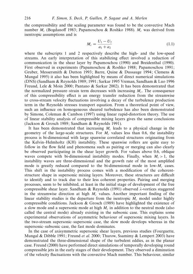
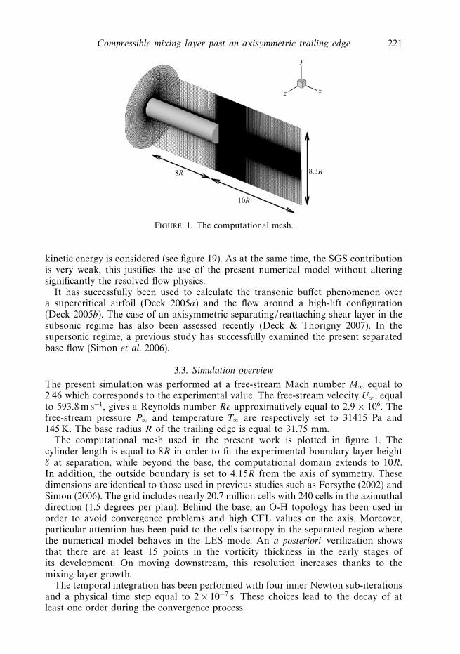
Figure 2. Supersonic base flow topology (iso-lines of pressure and computed streamlines).
The averaging process has been performed over a physical time equal to 75 mswhich represents slightly less than 80 flow-through times. Based on the estimationof 1 µs per iteration and per grid cell, the simulation cost is equal to approximately8650 CPU hours on a NEC SX6 processor. In addition to the time-averaged flowfield, nearly 430 sensors were also placed in all the relevant areas of the near wake inorder to measure the dominant frequencies of the flow. The sampling rate is equal to250 kHz.
4. ValidationThe time-averaged flow field is depicted in figure 2 which highlights the classical
topology of the near wake in supersonic blunt-base flows. The incoming turbulentboundary layer separates at the base after passing through an expansion fan shownby the iso-contours of pressure. The free shear flow transforms into a mixing layerexhibiting high compressibility levels. On moving downstream, the mixing processinside the shear layer leads to an equilibrium between the free stream and the low-pressure region behind the trailing edge which represents the recirculating area (alsocalled the ‘dead-air region’ despite its unsteady nature). The streamline curvature inthe shear flow then decreases due to the axisymmetric constraint for 1.8 <x/R < 4.On realigning with the axis, part of the incoming flow has enough momentum to passthrough the recompression and to be convected downstream into a turbulent wake.The compression waves coalesce in the free stream and form a recompression shock.The other part of the flow is pushed upstream thus forming a toroidal reverse flowtopology. This recirculating region extends to approximately 2.7R (= LR) which agreesvery well with the experimental value of 2.67R. The streamline which represents theboundary between the recirculation region and the free stream is called the dividingstreamline and its intersection with the axis is named the rear stagnation point.
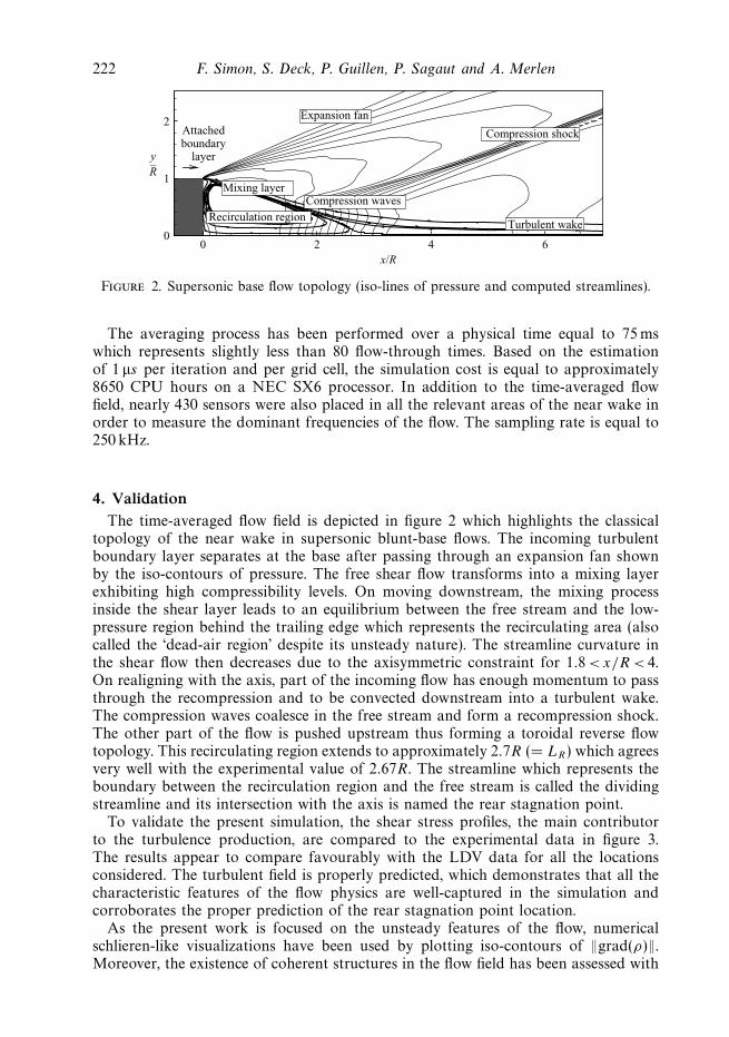
To validate the present simulation, the shear stress profiles, the main contributorto the turbulence production, are compared to the experimental data in figure 3.The results appear to compare favourably with the LDV data for all the locationsconsidered. The turbulent field is properly predicted, which demonstrates that all thecharacteristic features of the flow physics are well-captured in the simulation andcorroborates the proper prediction of the rear stagnation point location.
As the present work is focused on the unsteady features of the flow, numericalschlieren-like visualizations have been used by plotting iso-contours of ‖grad(ρ)‖.Moreover, the existence of coherent structures in the flow field has been assessed with
Compressible mixing layer past an axisymmetric trailing edge 223
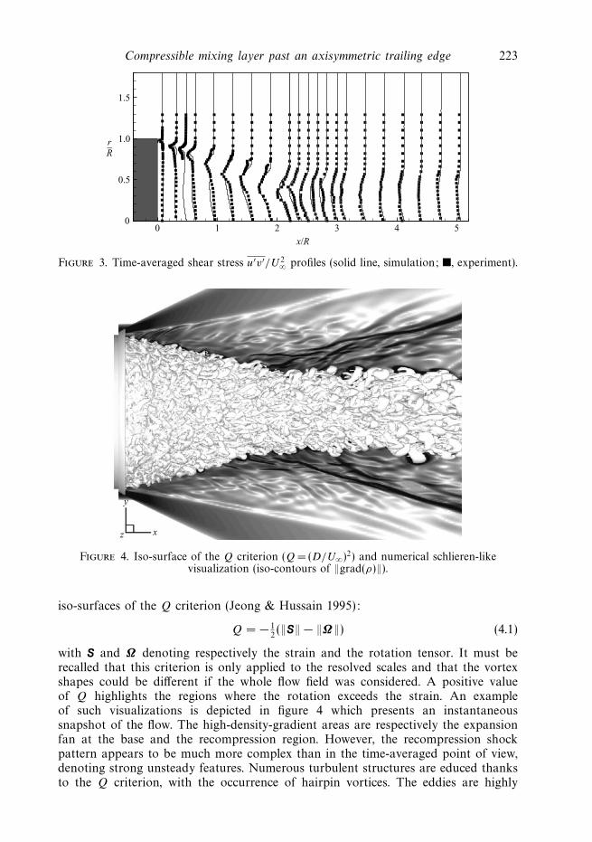
Figure 4. Iso-surface of the Q criterion (Q = (D/U∞)2) and numerical schlieren-likevisualization (iso-contours of ‖grad(ρ)‖).
iso-surfaces of the Q criterion (Jeong & Hussain 1995):
Q = − 12(‖S‖ − ‖Ω‖) (4.1)
with S and Ω denoting respectively the strain and the rotation tensor. It must berecalled that this criterion is only applied to the resolved scales and that the vortexshapes could be different if the whole flow field was considered. A positive valueof Q highlights the regions where the rotation exceeds the strain. An exampleof such visualizations is depicted in figure 4 which presents an instantaneoussnapshot of the flow. The high-density-gradient areas are respectively the expansionfan at the base and the recompression region. However, the recompression shockpattern appears to be much more complex than in the time-averaged point of view,denoting strong unsteady features. Numerous turbulent structures are educed thanksto the Q criterion, with the occurrence of hairpin vortices. The eddies are highly
224 F. Simon, S. Deck, P. Guillen, P. Sagaut and A. Merlen
x/LR
Num
ber
of s
truc
ture
s
0.4 0.8 1.2 1.60
10
20
30
40
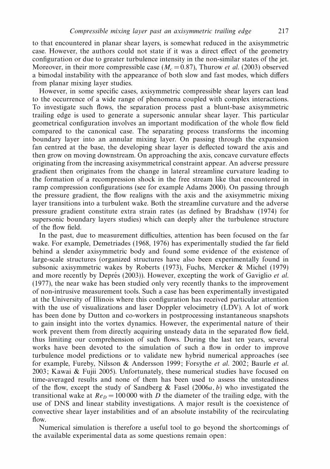
Figure 5. Estimation of the number of structures in the azimuthal direction (dashed line,simulation; , experiment; grey area, RMS experimental value).
three-dimensional and appear to grow in size farther downstream leading to areduction of the number of vortices.
Figure 5 depicts the streamwise evolution of the number of eddies in the azimuthaldirection along the shear layer and the results are compared to the experimental dataof Bourdon & Dutton (2001).
Despite only one time instant being used for the present estimation, the numericalobservations compare well with the experimental results and properly predict thereduction in the number of eddies as the recirculation area shrinks. This is furtherevidence that the simulation can be used to investigate the vortex dynamics.
Thus, the present simulation exhibits most of the features observable in theexperiment and will now be used to obtain a better insight into the dynamics ofthe flow.
5. Mixing layer analysis for 0 < x/LR < 0.60
5.1. Mean flow analysis
The time-averaged behaviour of the free shear layer was first investigated andparticular attention was paid to the mixing layer growth. Consequently, the vorticitythickness δω has been used:
δω(x, θ) =U
(∂u(x, r, θ)/∂r)max
(5.1)
with U = U1 − U2.
The evolution of δω behind the base is plotted in figure 6 where three distinct zonescan seen. The first region just after separation extends to approximately 0.3 x/LR andexhibits a growth rate dδω/dx approximately equal to 0.25. This region corresponds tothe initial part of the shear layer where instabilities develop. On moving downstream,dδω/dx increases until reaching a value equal to 0.38. This large value departs fromthe classical values encountered in canonical shear layers. However, this quite highspreading rate is due to the existence of the recirculating flow which involves highturbulence levels on the low-speed side as already observed in planar incompressibleseparating/reattaching flows (Dandois, Garnier & Sagaut 2007) as well as in subsonic
Compressible mixing layer past an axisymmetric trailing edge 225
x/LR
δω—R
0.2 0.4 0.6 0.8 1.0 1.2 1.40
0.2
0.4
0.6ComputationExp.
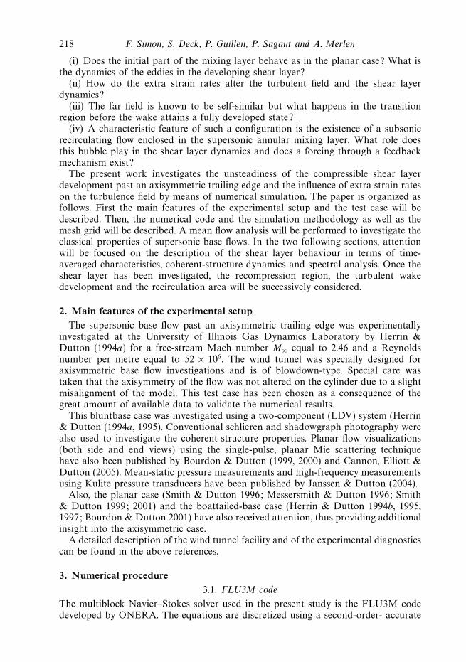
Figure 6. Vorticity thickness evolution along the mixing layer.
axisymmetric cases under moderate compressibility (Deck & Thorigny 2007 andSimon et al. 2007). For example, the latter showed that high values of the mixinglayer spreading rate are also observed in massively separated base flows for projectileconfigurations in the subsonic and transsonic regimes. At x/LR ∼ 0.60, a strongchange in the mixing layer evolution is observed. The vorticity thickness becomesnearly constant until the rear stagnation point at x/LR = 1 is reached. This shift inthe trend of the growth rate is due to the appearance of an adverse pressure gradientwhen the flow starts to realign with the axis as observed in figure 2. It can be notedthat the numerical results agree fairly well with the experimental values extractedfrom the LDV data.
For canonical shear layers, the vorticiy thickness growth rate can be defined by therelation
dδw
dx= Cδ
U1 − U2
U1 + U2
. (5.2)
However, due to the present configuration and the existence of recirculating flow,this formula does not strictly hold and leads to a Cδ value which is dependent uponthe streamwise location (for dδw/dx ∼ 0.38, Cδ(x) varies from 0.14 to 0.16, the latterbeing the classical incompressible value for planar shear layers).
For the purpose of better understanding the turbulence field modifications, thestreamwise evolution of the peak Reynolds stress magnitudes |u′
iu′j |max/U 2
∞ have beeninvestigated. Figure 7 presents the primary shear stress and both the axial and radialcomponents of the stress tensors.
The −u′v′/U 2∞ component results compare fairly well with the experimental data. In
accordance with the shear layer growth, the primary Reynolds shear stress magnitudesrise by a factor of 2 between x/LR =0.05 and 0.6. The onset of the recompressionregion appears to deeply alter the turbulence field as the primary stresses start tomonotically decrease from this location. This is consistent with the observations ofHerrin & Dutton (1997) and confirms that the turbulence immediately reacts to thepressure gradient which constitutes an extra strain rate, and contrasts with conclusionsabout subsonic flows.
The evolution of the streamwise component u′2/U 2∞, depicted in figure 7(b) can
be divided into four regions. For 0.05 <x/LR < 0.2, it decreases by nearly 16%.Then, its magnitude remains constant until x/LR =0.45. Downstream of this point,
226 F. Simon, S. Deck, P. Guillen, P. Sagaut and A. Merlen
x/LR
–u′v
′/U2 ∞
0.5 1.0 1.5 2.00
0.01
0.02
0.03
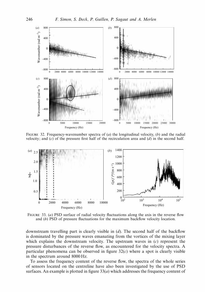
0.04
0.05Computation
Exp.
u′2 /U
2 ∞
x/LR
0.5 1.0 1.5 2.00
0.01
0.02
0.03
0.04
0.05
x/LR
0.5 1.0 1.5 2.00
0.01
0.02
0.03
0.04
0.05
v′2 /U
2 ∞
Figure 7. Longitudinal evolution of the peak Reynolds stresses: (a) −u′v′/U 2∞, (b) u′2/U 2
∞and (c) v′2/U 2
∞.
u′2/U 2∞ increases until the onset of recompression. Once again, the axial normal stress
responds instantaneously to the adverse pressure gradient. Figure 7(c) presents theevolution of the radial normal stress. Its magnitude is less than that of the axial stressand corroborates the finding of the domination of streamwise velocity fluctuations insuch flows (see for example Olsen & Dutton 2003; Goebel & Dutton 1990, Samimy &Elliot 1990, Urban & Mungal 2001); it exhibits a different behaviour than u′2/U 2
∞ in
the initial stage of the shear layer. The magnitude of v′2/U 2∞ is found to increase until
the recompression point is reached. Although not shown here, both the magnitudeand evolution of w′2/U 2
∞ are similar to those of v′2/U 2∞.
Table 1 summarizes some interesting properties of the turbulent field encounteredin classical shear flows as well as those encountered in the present simulation. Itillustrates the decrease of the fluctuation magnitude with Mc in canonical shear flowswhile the anisotropy is found to increase.
Because of the different evolution of the peak Reynolds stresses along the mixinglayer, it is interesting to investigate some particular ratios which depict the structuralchanges of the turbulent field due to the application of the extra strain rates.Figure 8(a) depicts the evolution of the Reynolds stress anisotropy through a primary-to-secondary stress ratio (σu/σv)
2 and a secondary-to-secondary stress ratio (σw/σv)2.
These ratios, measured at the peak shear stress location, exhibit two distinct trends.The first ratio underlines the domination of the axial stress in the whole turbulent field.However, (σu/σv)
2 is nearly equal to 3 downstream of separation and quickly decays to
Compressible mixing layer past an axisymmetric trailing edge 227
Topology EXP SIM Mc urms/u vrms/u√
u′v′/u vrms/urms
√u′v′/urms
Friedrich & Arnal(1990) BFS x – 0.224 0.141 0.126 0.629 0.562
Bell & Mehta (1990) PML x ∼0.00 0.18 0.14 0.10 0.777 0.555
Jovic (1996) BFS x ∼0.02 0.2 0.148 0.122 0.74 0.61
Freund, Lele & Moin(2000) AML x 1.80 0.205 0.055 0.063 0.268 0.307
Present simulation x 0.140 0.117 0.106 0.836 0.714
Table 1. Comparison of peak Reynolds stresses in classical shear flows: PML denotes planarshear layer, AML axisymmetric mixing layer, and BFS backward-facing step
x/LR
Nor
mal
str
ess
anis
otro
py r
atio
0 0.2 0.4 0.6 0.8 1.0 1.2 1.4
0.5
1.0
1.5
2.0
2.5
3.0(σu/σv)
2
(σw/σv)2
Tur
bule
nce
stru
ctur
e pa
ram
eter
0.2
0.4
0.6
0.8
1.0–u′v′/kRuv
x/LR
0 0.2 0.4 0.6 0.8 1.0 1.2 1.4
Figure 8. Longitudinal evolution of the normal shear stress anisotropy (a) and of theturbulence structure parameter (b) along the mixing layer.
approximately 1.2 at x/LR = 0.5, denoting a larger growth of the radial fluctuationscompared to the longitudinal ones. Farther downstream, this value remains constantthrough the recompression process and the developing wake, assuming that someequilibrium state has been reached. The 1.2 value is significantly lower than in planarshear layers mentioned in table 1. However, in the present case, both high- and low-speed stream characteristics evolve in the streamwise direction due to the existenceof the recirculating flow. Such spatial evolution greatly differs from canonical mixinglayers. In addition, the low-speed side is altered by the existence of the recirculation
228 F. Simon, S. Deck, P. Guillen, P. Sagaut and A. Merlen
x/LR
Cp r
ms m
ax
0.25 0.50 0.75 1.00 1.25 1.500
0.01
0.02
0.03
0.04
Figure 9. Streamwise evolution of the maximum pressure fluctuations coefficient Cprmsmaxin
the mixing layer.
area which enhances its turbulence level. Owing to these considerations, a strictcomparison between the axisymmetric and the planar cases is quite difficult. Thesecond ratio, (σw/σv)
2, remains nearly constant along the mixing layer independentlyof the additional strain rates. Its value is slightly larger than 1 in accordance with theresults of Herrin & Dutton (1997) in the case of an axisymmetric, boat-tailed trailingedge.
In addition to the normal shear stress distribution, some others relevant ratioscan be studied. As stated by Herrin & Dutton (1997), shear-stress-to-normal stressratio may be used for Reynolds stress closure. Two turbulence structure parametersare plotted in figure 8(b). The first ratio is −u′v′/k where k is the turbulent kineticenergy defined as k = (σ 2
u + σ 2v + σ 2
w)/2. The second one, commonly called the shearstress correlation coefficient, is Ruv = (−u′v′)/(σuσv). Both ratios exhibit the sameevolution despite different magnitudes. A strong decay is observed until x/LR = 1 andan asymptotic level is then reached. This contrasts with the experimental observationof Herrin & Dutton (1997) where no equilibrium state is reached at least untilx/LR = 1.5 when a boat-tailed trailing edge is used to generate the annular mixinglayer. The −u′v′/k ratio has a constant value of 0.4 which is slightly higher than thevalue of 0.3 recommended by Harsha & Lee (1970) for turbulent flow calculations.The Ruv ratio magnitude of approximately 0.6 agrees well with the results of Urban& Mungal (2001) for Mc = 0.63.
To conclude the study of the mean properties of the shear layer before enteringthe recompression region, the maximum of the pressure fluctuations have beeninvestigated and plotted in figure 9. It can be seen that pressure fluctuation maximaare nearly constant for 0 < x/XR < 0.5 with Cprmsmax
∼ 0.01. This behaviour differsfrom those observed in subsonic compressible base flows such as in Deck, Garnier &Guillen (2002), where the pressure maxima quickly increase during the early stages ofdevelopment of the shear layer and reach a value of approximatly 0.07 (for M∞ = 0.7),which is much higher than the constant value observed in the present case.
5.2. Coherent structure dynamics
In the previous section, the turbulence field has been investigated by means ofthe time-averaged data and its behaviour has been highlighted. Instantaneous data
Compressible mixing layer past an axisymmetric trailing edge 229
1.2
1.0
0.8
0.50 0.2 0.4 0.6
x/R0.8 1.0
yR
Figure 10. Visualization of radiating pressure waves on the upper side of the vorticeseduced using ∂ρ/∂x.
will now be used to investigate the turbulence properties through the existence andevolution of coherent vortices along the mixing layer.
The initial stage of the shear layer is first investigated. Figure 4 depicts the iso-surface of the Q criterion. The present case differs from the incompressible shear layercases where large spanwise rollers are observed due to the domination of the classicalKH instability. The small scales appear to be highly three-dimensional. Indeed, afterseparation, the compressibility effects are strong and the local convective Machnumber is greater than 1. It has been demonstrated (see for example Sandham &Reynolds 1991) that the shear layer is no longer dominated by the Kelvin–Helmholtzinstability. When Mc > 1, oblique modes dominate the instability process, leading tosmall-scale three-dimensional structures. The angle of the structure with the axis ofthe mean flow is dependent on the Mc value. Sandham & Reynolds (1991) have usedthe linear stability theory to educe a relation between Mc and the preferred mode forplanar shear layers:
Mc cos(θ) ∼ 0.6. (5.3)
Even though an averaged structure angle has not been clearly found in thesimulation, the visualization of figure 4 clearly shows highly three-dimensionalvortices, inclined toward the axis and with a weak azimuthal coherency.
The streamwise derivative of the density is used to show the vicinity of the separationprocess in figure 10. The white area depicts the expansion fan centred at the basewhich deflects the separating boundary layer. It is obvious that coherent vortices existin the shear layer just downstream of the base. Further evidence of their existence isfound in the pressure waves emanating from their upper side. Some eddies are seenalong the trailing edge and a small recirculation area is educed in the outer part ofthe base. These observations are consistent with the strong growth rate of the mixinglayer which can be forced by the impact of vortices coming from the recirculationbubble.
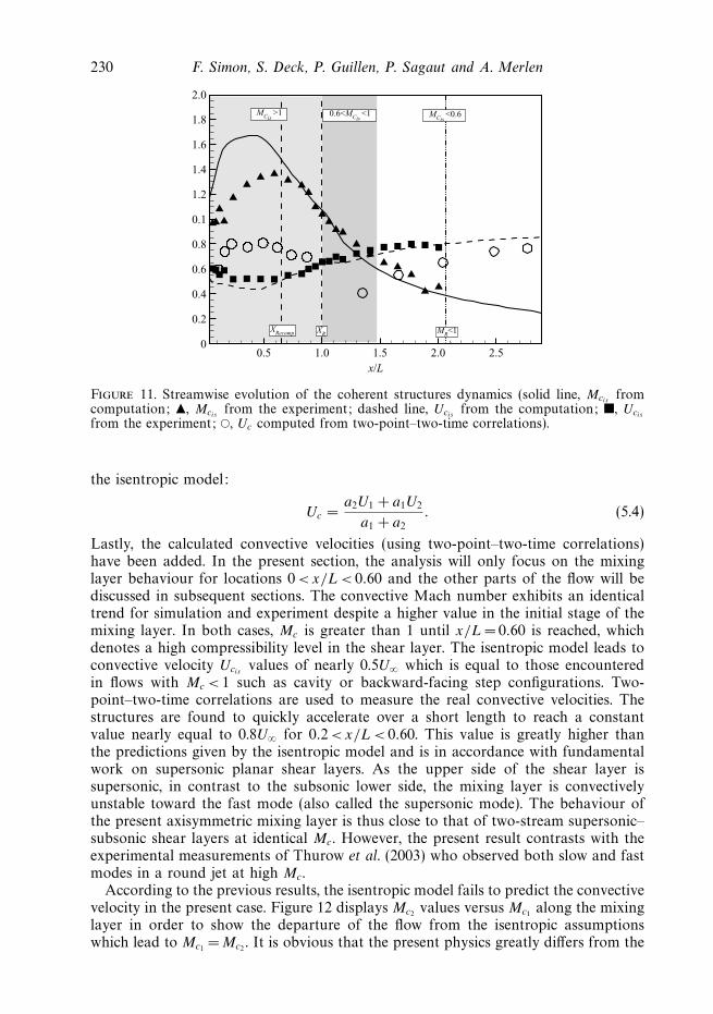
As the existence of coherent vortices has been demonstrated in the developing shearlayer, it is of primary interest to investigate their convective velocity Uc in order toestimate the relevance of the isentropic model of Uc. An estimation of the isentropicconvective Mach number Mc has been plotted in figure 11 and compared to theexperimental values. The convective velocity has also been estimated with the use of
230 F. Simon, S. Deck, P. Guillen, P. Sagaut and A. Merlen
2.0
1.8
1.6
1.4
1.2
0.1
0.8
0.6
0.4
0.2
00.5 1.0 1.5
x/L2.0
MR<1
2.5
XRXRecomp
MCis >1 0.6<MCis <1 MCis <0.6
Figure 11. Streamwise evolution of the coherent structures dynamics (solid line, Mcisfrom
computation; , Mcisfrom the experiment; dashed line, Ucis
from the computation; , Ucis
from the experiment; , Uc computed from two-point–two-time correlations).
the isentropic model:
Uc =a2U1 + a1U2
a1 + a2
. (5.4)
Lastly, the calculated convective velocities (using two-point–two-time correlations)have been added. In the present section, the analysis will only focus on the mixinglayer behaviour for locations 0 <x/L < 0.60 and the other parts of the flow will bediscussed in subsequent sections. The convective Mach number exhibits an identicaltrend for simulation and experiment despite a higher value in the initial stage of themixing layer. In both cases, Mc is greater than 1 until x/L = 0.60 is reached, whichdenotes a high compressibility level in the shear layer. The isentropic model leads toconvective velocity Ucis
values of nearly 0.5U∞ which is equal to those encounteredin flows with Mc < 1 such as cavity or backward-facing step configurations. Two-point–two-time correlations are used to measure the real convective velocities. Thestructures are found to quickly accelerate over a short length to reach a constantvalue nearly equal to 0.8U∞ for 0.2 <x/L < 0.60. This value is greatly higher thanthe predictions given by the isentropic model and is in accordance with fundamentalwork on supersonic planar shear layers. As the upper side of the shear layer issupersonic, in contrast to the subsonic lower side, the mixing layer is convectivelyunstable toward the fast mode (also called the supersonic mode). The behaviour ofthe present axisymmetric mixing layer is thus close to that of two-stream supersonic–subsonic shear layers at identical Mc. However, the present result contrasts with theexperimental measurements of Thurow et al. (2003) who observed both slow and fastmodes in a round jet at high Mc.
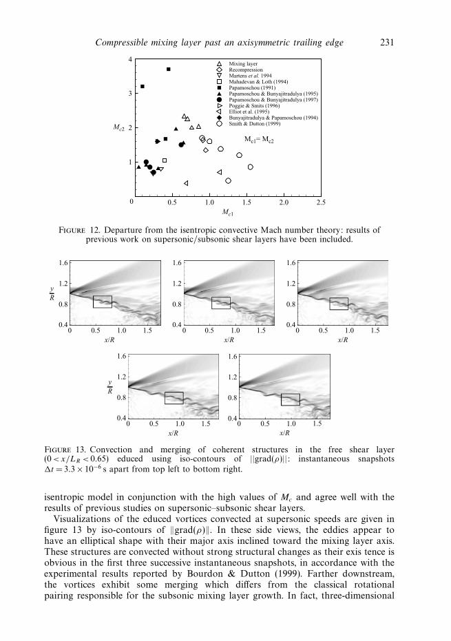
According to the previous results, the isentropic model fails to predict the convectivevelocity in the present case. Figure 12 displays Mc2
values versus Mc1along the mixing
layer in order to show the departure of the flow from the isentropic assumptionswhich lead to Mc1
= Mc2. It is obvious that the present physics greatly differs from the
Compressible mixing layer past an axisymmetric trailing edge 231
Figure 12. Departure from the isentropic convective Mach number theory: results ofprevious work on supersonic/subsonic shear layers have been included.
1.6
1.2
0.8
0.40 0.5
x/Rx/R
x/R x/R
x/R1.0 1.5
1.6
1.2
0.8
0.40 0.5 1.0 1.5
1.6
1.2
0.8
0.40 0.5 1.0 1.5
1.6
1.2
0.8
0.40 0.5 1.0 1.5
1.6
1.2
0.8
0.40 0.5 1.0 1.5
yR
yR
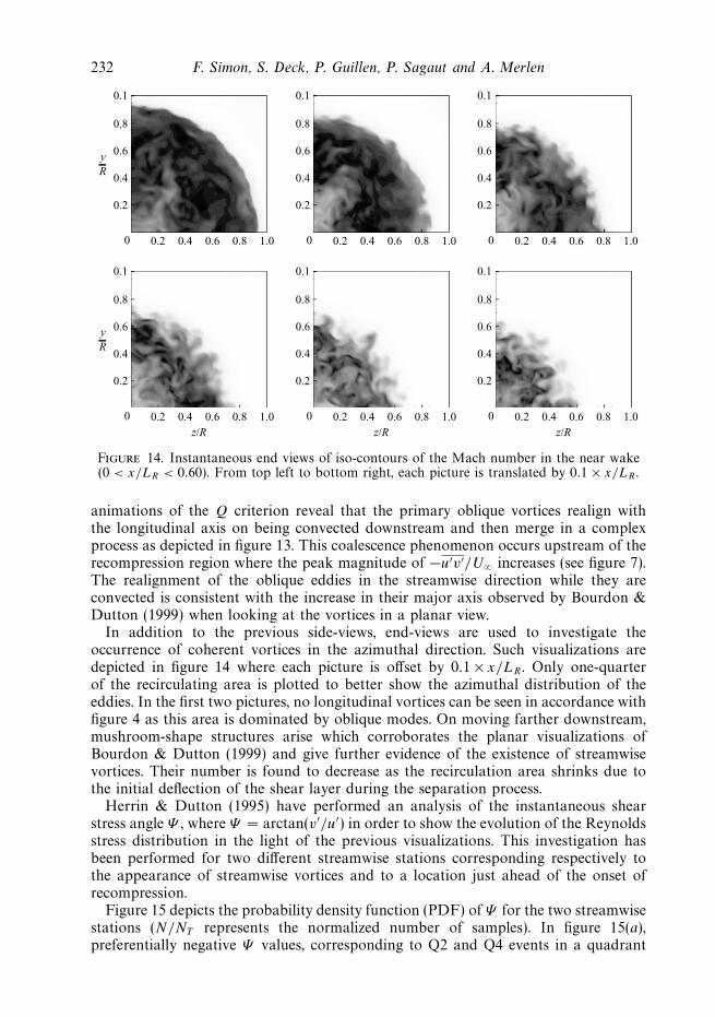
Figure 13. Convection and merging of coherent structures in the free shear layer(0 <x/LR < 0.65) educed using iso-contours of ||grad(ρ)||: instantaneous snapshotst = 3.3 × 10⁻⁶ s apart from top left to bottom right.
isentropic model in conjunction with the high values of Mc and agree well with theresults of previous studies on supersonic–subsonic shear layers.
Visualizations of the educed vortices convected at supersonic speeds are given infigure 13 by iso-contours of ‖grad(ρ)‖. In these side views, the eddies appear tohave an elliptical shape with their major axis inclined toward the mixing layer axis.These structures are convected without strong structural changes as their exis tence isobvious in the first three successive instantaneous snapshots, in accordance with theexperimental results reported by Bourdon & Dutton (1999). Farther downstream,the vortices exhibit some merging which differs from the classical rotationalpairing responsible for the subsonic mixing layer growth. In fact, three-dimensional
232 F. Simon, S. Deck, P. Guillen, P. Sagaut and A. Merlen
0.1
0.8
0.6
0.4
0.2
0 0.2 0.4 0.6 0.8 1.0
0.1
0.8
0.6
0.4
0.2
0 0.2 0.4z/R z/R z/R
0.6 0.8 1.0
0.1
0.8
0.6
0.4
0.2
0 0.2 0.4 0.6 0.8 1.0
0.1
0.8
0.6
0.4
0.2
0 0.2 0.4 0.6 0.8 1.0
0.1
0.8
0.6
0.4
0.2
0 0.2 0.4 0.6 0.8 1.0
0.1
0.8
0.6
0.4
0.2
0 0.2 0.4 0.6 0.8 1.0
yR
yR
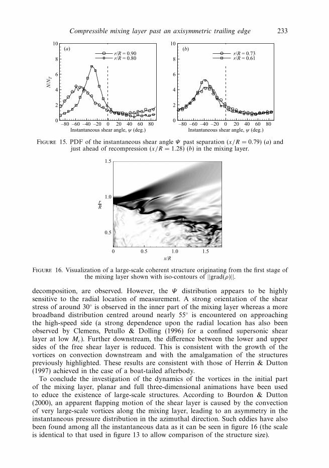
Figure 14. Instantaneous end views of iso-contours of the Mach number in the near wake(0 < x/LR < 0.60). From top left to bottom right, each picture is translated by 0.1 × x/LR .
animations of the Q criterion reveal that the primary oblique vortices realign withthe longitudinal axis on being convected downstream and then merge in a complexprocess as depicted in figure 13. This coalescence phenomenon occurs upstream of therecompression region where the peak magnitude of −u′v′/U∞ increases (see figure 7).The realignment of the oblique eddies in the streamwise direction while they areconvected is consistent with the increase in their major axis observed by Bourdon &Dutton (1999) when looking at the vortices in a planar view.
In addition to the previous side-views, end-views are used to investigate theoccurrence of coherent vortices in the azimuthal direction. Such visualizations aredepicted in figure 14 where each picture is offset by 0.1 × x/LR . Only one-quarterof the recirculating area is plotted to better show the azimuthal distribution of theeddies. In the first two pictures, no longitudinal vortices can be seen in accordance withfigure 4 as this area is dominated by oblique modes. On moving farther downstream,mushroom-shape structures arise which corroborates the planar visualizations ofBourdon & Dutton (1999) and give further evidence of the existence of streamwisevortices. Their number is found to decrease as the recirculation area shrinks due tothe initial deflection of the shear layer during the separation process.
Herrin & Dutton (1995) have performed an analysis of the instantaneous shearstress angle Ψ , where Ψ = arctan(v′/u′) in order to show the evolution of the Reynoldsstress distribution in the light of the previous visualizations. This investigation hasbeen performed for two different streamwise stations corresponding respectively tothe appearance of streamwise vortices and to a location just ahead of the onset ofrecompression.
Figure 15 depicts the probability density function (PDF) of Ψ for the two streamwisestations (N/NT represents the normalized number of samples). In figure 15(a),preferentially negative Ψ values, corresponding to Q2 and Q4 events in a quadrant
Compressible mixing layer past an axisymmetric trailing edge 233
Figure 15. PDF of the instantaneous shear angle Ψ past separation (x/R = 0.79) (a) andjust ahead of recompression (x/R = 1.28) (b) in the mixing layer.
1.5
0.5
0 0.5x/R
1.0 1.5
1.0rR
Figure 16. Visualization of a large-scale coherent structure originating from the first stage ofthe mixing layer shown with iso-contours of ||grad(ρ)||.
decomposition, are observed. However, the Ψ distribution appears to be highlysensitive to the radial location of measurement. A strong orientation of the shearstress of around 30 is observed in the inner part of the mixing layer whereas a morebroadband distribution centred around nearly 55 is encountered on approachingthe high-speed side (a strong dependence upon the radial location has also beenobserved by Clemens, Petullo & Dolling (1996) for a confined supersonic shearlayer at low Mc). Further downstream, the difference between the lower and uppersides of the free shear layer is reduced. This is consistent with the growth of thevortices on convection downstream and with the amalgamation of the structurespreviously highlighted. These results are consistent with those of Herrin & Dutton(1997) achieved in the case of a boat-tailed afterbody.
To conclude the investigation of the dynamics of the vortices in the initial partof the mixing layer, planar and full three-dimensional animations have been usedto educe the existence of large-scale structures. According to Bourdon & Dutton(2000), an apparent flapping motion of the shear layer is caused by the convectionof very large-scale vortices along the mixing layer, leading to an asymmetry in theinstantaneous pressure distribution in the azimuthal direction. Such eddies have alsobeen found among all the instantaneous data as it can be seen in figure 16 (the scaleis identical to that used in figure 13 to allow comparison of the structure size).
234 F. Simon, S. Deck, P. Guillen, P. Sagaut and A. Merlen
2.2
1.7
1.2
0.7
0.20 2 4 6
Frequency (Hz)8 10 12(×104)
xRecomp
xR
Figure 17. Spectral surface of longitudinal velocity fluctuations (Gu(f ) ∗ f/σ 2u ) along the
mixing layer.
Such an eddy is significantly larger than the vortices educed in figure 13 andcorroborates the experimental findings. However, no clear periodic nature in theiroccurrence has been found and a spectral analysis is required in order to showpossible periodic motions in the mixing layer.
5.3. Spectral analysis
Some additional knowledge can be obtained by performing a spectral analysis ofthe mixing layer. Such an investigation has been performed by plotting the spectralsurface of the longitudinal velocity fluctuations along the mixing layer using 23sensors in figure 17.
The present analysis focuses on the mixing layer behaviour ahead of therecompression. Two distinct areas can be seen: downstream of separation, the initialstage of the shear layer displays a high-frequency content corresponding to the primaryinstability of the mixing layer unlike downstream locations where the spectral contentis pushed toward lower frequencies in accordance with the growth and amalgation ofthe convected vortices along the shear layer.
Two characteristic spectra coming from the previous spectral surface can be seenin figure 18. Figure 18(a) depicts a spectrum of velocity fluctuations downstreamof separation. As mentioned earlier, the high-frequency content, centred aroundapproximately 60 kHz, is the signature of the instability process of the shear layer.This frequency is also encountered in the radial velocity fluctuation spectra and inthe temporal autocorrelation coefficients. However, it is obvious that, at this location,the shear layer has a low-frequency component. A peak is observed at 1350 Hz(StD ∼ 0.144) but energy is relatively constant until 700 Hz. A similar frequency isobserved in radial and tangential velocity spectra despite the lower value of 900 Hz(StD ∼ 0.096). This quite low frequency does not scale with the mixing layer propertiesand may be characteristic of a global behaviour of the whole flow just downstreamof separation. As previously discussed, a flapping motion of the shear layer is a goodcandidate for this frequency.
Figure 18(b) exhibits the longitudinal velocity spectrum just ahead of recompressionin the mixing layer. It is observed that the high-frequency component has spread to
Compressible mixing layer past an axisymmetric trailing edge 235
0.7(a) (b)
0.6
0.5
0.4
Gu(
f)∗f
/σ2 u
0.3
0.2
0.1
0102
0.7
0.6
0.5
0.4
Gu(
f)∗f
/σ2 u
0.3
0.2
0.1
0102103
Frequency (Hz) Frequency (Hz)104 105 103 104 105
Figure 18. Longitudinal velocity spectra (a) in the initial part of the mixing layer for x/R =0.25 and y/R = 0.97 and (b) ahead of the recompression region for x/R = 1.52 and y/R = 0.61.
lower frequencies corresponding to the growth of the vortices as they are convected.The spectrum exhibits a broadband shape with maximum fluctuations around 25 kHz(this value is a little higher for the radial and tangential velocity fluctuations).In addition, a small peak is observed at a frequency corresponding to 800 Hz(StD ∼ 0.085). Movements of the whole separated flow enclosed in the annular shearlayer have been experimentally observed for frequencies below 1 kHz (Cannon et al.2005). The present work gives further evidence of the existence of such large-scalebehaviour.
To summarize, the present section is devoted to the mixing layer propertiesahead of the recompression. An investigation of the time-averaged flow field hashighlighted the strong growth rate of the shear layer coupled with a dominationof the streamwise velocity fluctuations. Instantaneous samples have demonstratedthe existence of numerous turbulent scales. As a result of the compressibility of theflow, the isentropic model of the convective Mach number fails to predict the vortexdynamics which appear to be linked to the supersonic mode. A spectral analysis givesthe frequency of the shear layer instability as well as a low-frequency phenomenonwhich appears to be related to a flapping motion of the mixing layer. The next sectionwill assess the shear layer properties during the recompression process as well as thedynamics of the complex shock pattern educed in figure 4.
6. Turbulence structure in the recompression and in the rear stagnation region(0.6 < x/LR < 1)
6.1. Mean flow analysis
On moving downstream, the free shear layer develops closer to the axis andthe axisymmetrical constraints increase. For x/LR > 0.65, the lateral streamlineconvergence leads to recompression and to the formation of a compression shockfrom a time-averaged point of view as depicted in figure 2. The incoming fluidparticles having enough momentum pass through the recompression and then areconvected downstream into the developing wake. Those with less energy are pushedupstream into a backflow area which will be discussed in the last section.
The recompression process has a direct effect on the shear layer behaviour ashighlighted by the evolution of δω (see figure 6). A constant value of δω is observeduntil the rear stagnation point is reached, providing some evidence of the turbulence
236 F. Simon, S. Deck, P. Guillen, P. Sagaut and A. Merlen
0.03
0.030.03
0.050.05
0.190.19
0.19
0.19
0.360.39
2.0
1.5
0.1
0.5
00 1 2
x/R3 4 5
yR
Figure 19. Turbulent Mach number field based on the resolved turbulent kinetic energy.
field alteration. As observed in figure 7, the recompression region represents the onsetof the velocity fluctuation decrease. The parameter quantifying the compressibilityinfluence on the turbulent fluctuations is the turbulent Mach number Mt which caneither be defined with a root-mean-square (RMS) value of the longitudinal velocityfluctuation (u′2)1/2/a or with the resolved turbulent kinetic energy (k)1/2/a. Figure 19displays the Mt distribution and in particular non-negligable values in the recirculatingarea since Mt can reach values as high as 0.20. Moreover, its highest values are foundin the recompression region where Mt has values up to 0.36 or 0.40 depending on thescaling. At the present Mt levels (Mt < 0.6) and according to Erlebacher et al. (1992),the subgrid kinetic energy can be lumped with the pressure term as mentioned in§ 3.2.
The longitudinal and radial fluctuation components exhibit the same behaviourwhen passing through the recompression, allowing a constant value of the anisotropyparameter (σu/σv)
2 approximately equal to 1.25 due to the domination of thestreamwise fluctuations (see figure 7 and figure 8). Thus, the turbulence field intensitydecreases while the anisotropy of the flow remains constant. This is a quite differentbehaviour from that encountered in compressible turbulent reattaching free shearlayers such as in compression ramp configurations. On approaching the ramp, the freemixing layer enters a compression region leading to a modification of the turbulencefield. The velocity fluctuations are immediately enhanced and maximum fluctuationslevels are reached just downstream of the mean reattachment point (Samimy, Petrie& Addy 1986).
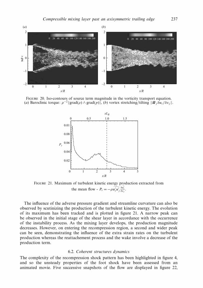
Finally, the pressure gradient resulting from the streamline curvature coupledwith density variations is responsible for another particular property of the presentconfiguration. One characteristic feature of compressible flows is the vorticitygeneration due to the baroclinic term in the vorticity transport equation. In the presentcase, the adverse pressure gradient is not aligned with the density variations acrossthe shear layer, which only appear in the radial direction. Thus, this area appears asa source of vorticity through the compressible term of the equation. Iso-contours ofthe baroclinic torque magnitude are compared to the vortex stretching/tilting term inan instantaneous snapshot (figure 20). It is obvious that the compressibility acts notonly in the recompression region but also during the whole mixing layer developmentand its effect on the vorticity generation is of the same order as the incompressiblesource term, at least in the shear layer.
Compressible mixing layer past an axisymmetric trailing edge 237
Figure 20. Iso-contours of source term magnitude in the vorticity transport equation.(a) Baroclinic torque: ρ−2‖grad(ρ) ∧ grad(p)‖, (b) vortex stretching/tilting ‖Ωj ∂ui/∂xj ‖.
0 0.5 1.0
xLR
1.5
0.01
0.08
0.06Pr
0.04
0.02
0 1 2x/R
3 4 5
Figure 21. Maximum of turbulent kinetic energy production extracted from
the mean flow - Pr = −ρu′iu
′j
∂u′i
∂xj.
The influence of the adverse pressure gradient and streamline curvature can also beobserved by scutinizing the production of the turbulent kinetic energy. The evolutionof its maximum has been tracked and is plotted in figure 21. A narrow peak canbe observed in the initial stage of the shear layer in accordance with the occurrenceof the instability process. As the mixing layer develops, the production magnitudedecreases. However, on entering the recompression region, a second and wider peakcan be seen, demonstrating the influence of the extra strain rates on the turbulentproduction whereas the reattachement process and the wake involve a decrease of theproduction term.
6.2. Coherent structures dynamics
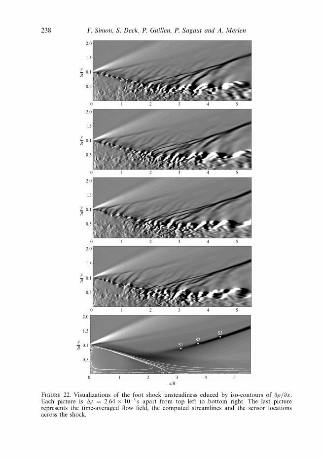
The complexity of the recompression shock pattern has been highlighted in figure 4,and so the unsteady properties of the foot shock have been assessed from ananimated movie. Five successive snapshots of the flow are displayed in figure 22,
238 F. Simon, S. Deck, P. Guillen, P. Sagaut and A. Merlen
2.0
1.5
0.1
0.5
0 1 2 3 4 5
2.0
1.5
0.1
0.5
0 1 2 3 4 5
2.0
1.5
0.1
0.5
0 1 2 3 4 5
2.0
1.5
0.1
0.5
0 1 2 3 4 5
2.0
1.5
0.1
0.5
0 1 2x/R
3 4 5
R
y
R
y
R
y
R
y
R
yS1
S2
S3
Figure 22. Visualizations of the foot shock unsteadiness educed by iso-contours of ∂ρ/∂x.Each picture is t = 2.64 × 10⁻⁵ s apart from top left to bottom right. The last picturerepresents the time-averaged flow field, the computed streamlines and the sensor locationsacross the shock.
Compressible mixing layer past an axisymmetric trailing edge 239
Skewness = 0.01Kurtosis = 3.05
Skewness = 0.74Kurtosis = 2.87
Skewness = 0.03Kurtosis = 3.13
1.0
0.8
(a) (b) (c)
0.6
0.4
0.2
0–4 –2 0 2 4
1.0
0.8
0.6
0.4
0.2
0–4 –2 0 2 4
1.0
0.8
0.6
0.4
0.2
0–4 –2 0 2 4
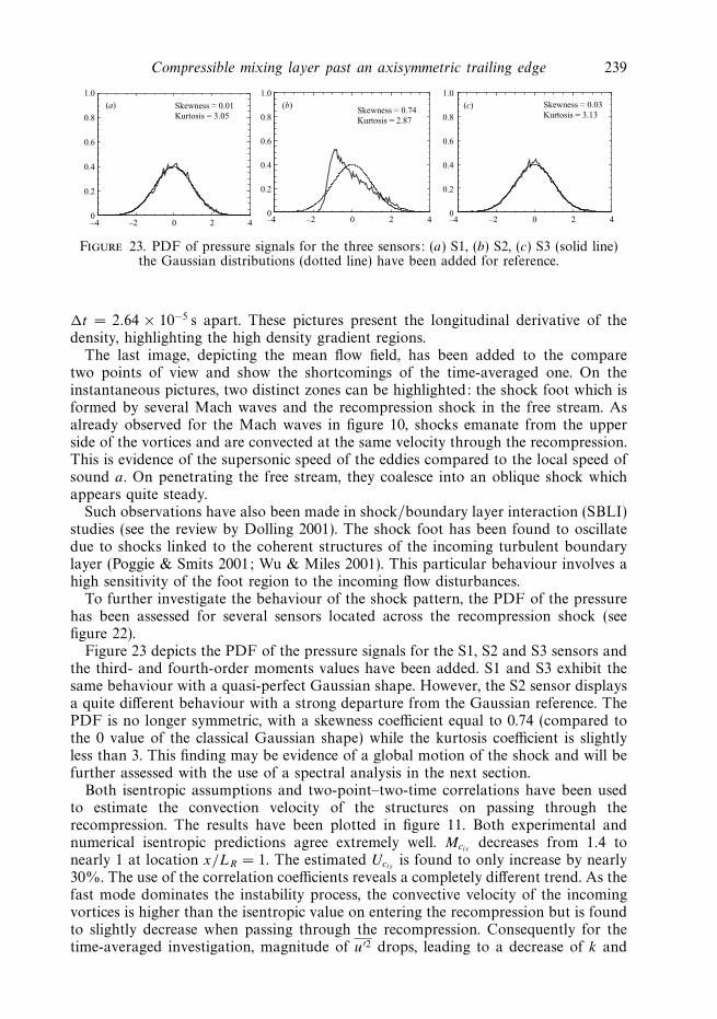
Figure 23. PDF of pressure signals for the three sensors: (a) S1, (b) S2, (c) S3 (solid line)the Gaussian distributions (dotted line) have been added for reference.
t = 2.64 × 10⁻⁵ s apart. These pictures present the longitudinal derivative of thedensity, highlighting the high density gradient regions.
The last image, depicting the mean flow field, has been added to the comparetwo points of view and show the shortcomings of the time-averaged one. On theinstantaneous pictures, two distinct zones can be highlighted: the shock foot which isformed by several Mach waves and the recompression shock in the free stream. Asalready observed for the Mach waves in figure 10, shocks emanate from the upperside of the vortices and are convected at the same velocity through the recompression.This is evidence of the supersonic speed of the eddies compared to the local speed ofsound a. On penetrating the free stream, they coalesce into an oblique shock whichappears quite steady.
Such observations have also been made in shock/boundary layer interaction (SBLI)studies (see the review by Dolling 2001). The shock foot has been found to oscillatedue to shocks linked to the coherent structures of the incoming turbulent boundarylayer (Poggie & Smits 2001; Wu & Miles 2001). This particular behaviour involves ahigh sensitivity of the foot region to the incoming flow disturbances.
To further investigate the behaviour of the shock pattern, the PDF of the pressurehas been assessed for several sensors located across the recompression shock (seefigure 22).
Figure 23 depicts the PDF of the pressure signals for the S1, S2 and S3 sensors andthe third- and fourth-order moments values have been added. S1 and S3 exhibit thesame behaviour with a quasi-perfect Gaussian shape. However, the S2 sensor displaysa quite different behaviour with a strong departure from the Gaussian reference. ThePDF is no longer symmetric, with a skewness coefficient equal to 0.74 (compared tothe 0 value of the classical Gaussian shape) while the kurtosis coefficient is slightlyless than 3. This finding may be evidence of a global motion of the shock and will befurther assessed with the use of a spectral analysis in the next section.
Both isentropic assumptions and two-point–two-time correlations have been usedto estimate the convection velocity of the structures on passing through therecompression. The results have been plotted in figure 11. Both experimental andnumerical isentropic predictions agree extremely well. Mcis
decreases from 1.4 tonearly 1 at location x/LR = 1. The estimated Ucis
is found to only increase by nearly30%. The use of the correlation coefficients reveals a completely different trend. As thefast mode dominates the instability process, the convective velocity of the incomingvortices is higher than the isentropic value on entering the recompression but is foundto slightly decrease when passing through the recompression. Consequently for thetime-averaged investigation, magnitude of u′2 drops, leading to a decrease of k and
240 F. Simon, S. Deck, P. Guillen, P. Sagaut and A. Merlen
0.8
0.6
0.4
0.2
0 0.2 0.4 0.6 0.8
0.8
0.6
0.4
0.2
0 0.2 0.4z/R z/R
0.6 0.8
0.8
0.6
0.4
0.2
0 0.2 0.4 0.6 0.8
0.8
0.6
0.4
0.2
0 0.2 0.4 0.6 0.8
yR
yR
Figure 24. Instantaneous end views of iso-contours of Mach number in the recompressionregion (0.70 <x/LR < 1). Each picture is offset by 0.1 ×/LR from top left to bottom right.
Instantaneous shear angle, Ψ (deg.)
x/R = 2.01, r/R = 0.54
x/R = 2.29, r/R = 0.49
x/R = 2.54, r/R = 0.43
10
8
6
4N/N
T (%
)
2
0–80 –60 –40 –20 0 20 40 60 80
Figure 25. PDF of the instantaneous shear stress angle Ψ along the mixing layer in therecompression region.
thus to a deceleration of the eddies. This result underlines the shortcomings of theisentropic model when a pressure gradient occurs in the flow field.
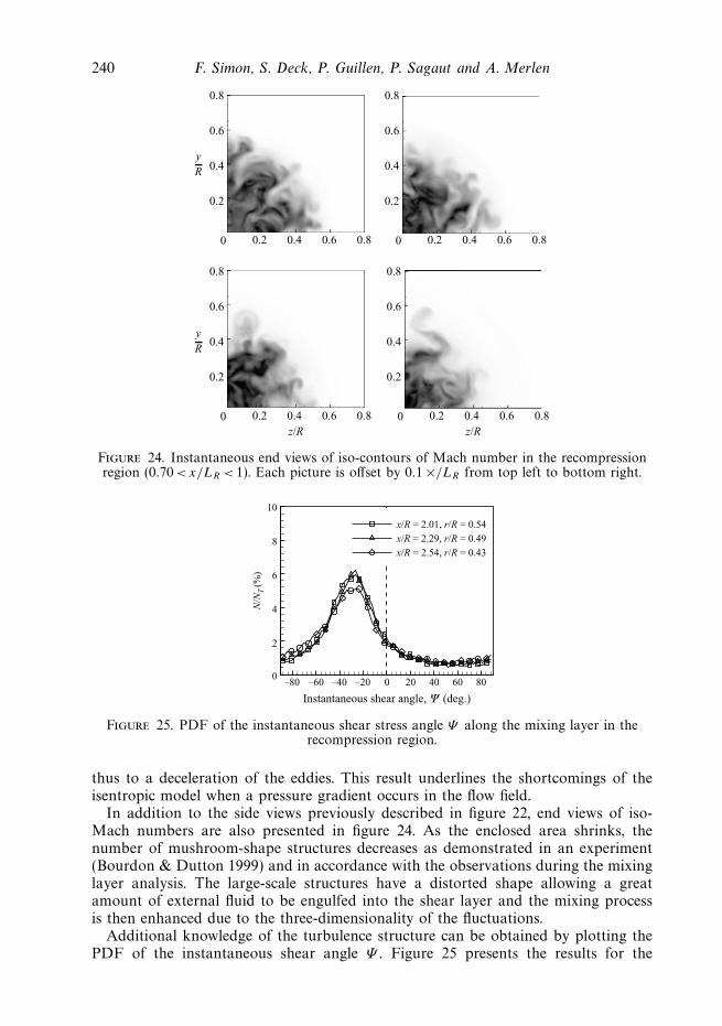
In addition to the side views previously described in figure 22, end views of iso-Mach numbers are also presented in figure 24. As the enclosed area shrinks, thenumber of mushroom-shape structures decreases as demonstrated in an experiment(Bourdon & Dutton 1999) and in accordance with the observations during the mixinglayer analysis. The large-scale structures have a distorted shape allowing a greatamount of external fluid to be engulfed into the shear layer and the mixing processis then enhanced due to the three-dimensionality of the fluctuations.
Additional knowledge of the turbulence structure can be obtained by plotting thePDF of the instantaneous shear angle Ψ . Figure 25 presents the results for the
Compressible mixing layer past an axisymmetric trailing edge 241
0.014
0.012
0.010
0.008
Gp(
f)∗f
σ2 p
0.006
0.004
0.002
0102 103
Freequency (Hz)104 105
S3
S2
S1
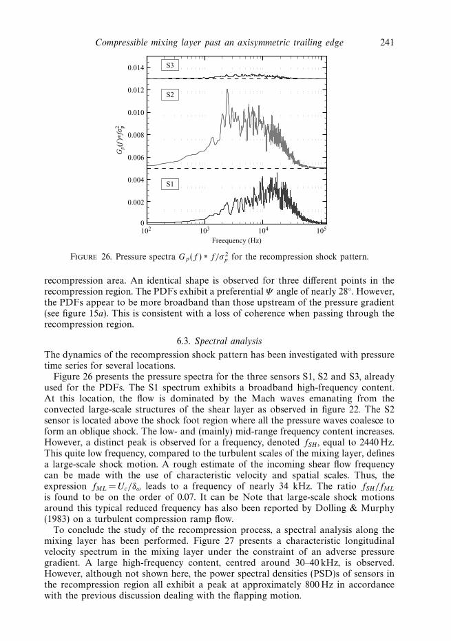
Figure 26. Pressure spectra Gp(f ) ∗ f/σ 2p for the recompression shock pattern.
recompression area. An identical shape is observed for three different points in therecompression region. The PDFs exhibit a preferential Ψ angle of nearly 28. However,the PDFs appear to be more broadband than those upstream of the pressure gradient(see figure 15a). This is consistent with a loss of coherence when passing through therecompression region.
6.3. Spectral analysis
The dynamics of the recompression shock pattern has been investigated with pressuretime series for several locations.
Figure 26 presents the pressure spectra for the three sensors S1, S2 and S3, alreadyused for the PDFs. The S1 spectrum exhibits a broadband high-frequency content.At this location, the flow is dominated by the Mach waves emanating from theconvected large-scale structures of the shear layer as observed in figure 22. The S2sensor is located above the shock foot region where all the pressure waves coalesce toform an oblique shock. The low- and (mainly) mid-range frequency content increases.However, a distinct peak is observed for a frequency, denoted fSH, equal to 2440 Hz.This quite low frequency, compared to the turbulent scales of the mixing layer, definesa large-scale shock motion. A rough estimate of the incoming shear flow frequencycan be made with the use of characteristic velocity and spatial scales. Thus, theexpression fML = Uc/δω leads to a frequency of nearly 34 kHz. The ratio fSH/fML
is found to be on the order of 0.07. It can be Note that large-scale shock motionsaround this typical reduced frequency has also been reported by Dolling & Murphy(1983) on a turbulent compression ramp flow.
To conclude the study of the recompression process, a spectral analysis along themixing layer has been performed. Figure 27 presents a characteristic longitudinalvelocity spectrum in the mixing layer under the constraint of an adverse pressuregradient. A large high-frequency content, centred around 30–40 kHz, is observed.However, although not shown here, the power spectral densities (PSD)s of sensors inthe recompression region all exhibit a peak at approximately 800 Hz in accordancewith the previous discussion dealing with the flapping motion.
242 F. Simon, S. Deck, P. Guillen, P. Sagaut and A. Merlen
0.7
0.6
0.5
0.4
0.3
0.2
0.1
102 103
Frequency (Hz)104 105
Gu(
f)∗σ
2 u
Figure 27. Longitudinal velocity spectra in the recompression region of the mixing layer atx/R = 2.17 and r/R = 0.52.
In summary, an investigation of the recompression process has shown that theadditional strain rate resulting from the lateral streamline convergence deeply altersthe turbulent field. The primary shear stress magnitude drops, as well as both the axialand radial velocity fluctuations, whereas the (σu/σv)
2 ratio remains constant. Froman instantaneous point of view, the shock pattern is revealed to be complex, with theshock foot formed by convected shocks emanating from the eddies contained in theshear layer. The vortex velocity is found to be reduced through the recompressionin contradiction with the prediction of the isentropic model. Finally, evidence of theexistence of a large-scale motion of the shock has been presented. Attention will nowturn to the investigation of the developing wake.
7. Wake region7.1. Mean flow analysis
The present section is focused on the transition region between the mixing layer andthe fully developed turbulent wake as far-field supersonic wakes are already known tobehave in a self-similar manner. As depicted in figure 7, velocity fluctuations continueto decay in the near wake while the anisotropy ratio remains constant (figure 8).Thus, the turbulent field seems to slowly evolve to an asympotic state correspondingto a fully developed supersonic wake. This transition is accompanied by a reductionof the compressibility level which can be shown with the relative Mach number Mr
parameter. Mr represents an estimation of the compressibility constraints of wakes(similarly to Mc for shear layers) and is given by
Mr =U∞ − Uaxis
a∞. (7.1)
Figure 28 depicts the streamwise evolution of Mr in the developing wake afterthe rear stagnation point. The Mr value quickly drops meaning that the centrelinevelocity significantly accelerates over a short distance. Beyond x/R ∼ 5.5, Mr is lessthan 1 and keeps decreasing. As Mr drops, the compressibility level decreases so thatthe wake properties should rapidly tend to those of its incompressible counterpartand reach a self-similar state.
Compressible mixing layer past an axisymmetric trailing edge 243
ComputationExp.
2.0
1.5
1.0
Mr
0.5
3 4 5 6
x/R
7 8 9 10
Figure 28. Evolution of the relative Mach number Mr in the developing turbulent wake.
7.2. Coherent structures dynamics
The decrease of the compressibility during the transition stage also appears inthe evolution of Mcis
(see figure 11). As Mcislevels drop, Ucis
is found to slightlyincrease. The measured convection velocity using two-time–two-point correlationsprovides lower values than the isentropic estimation which is consistent with thefluidic reattachment process. However, as Mr drops, Uc quickly increases until itnearly reaches the isentropic value of 0.8U∞ at x/LR = 3.
Concerning the structure of the wake, experimental visualizations (Bourdon &Dutton 1999, 2000) have demonstrated the highly convoluted nature of the developingwake. To compare the experimental observations to the present simulation, thestreamwise evolution of the wake is depicted in figure 29 for five different stationsafter the rear stagnation point.
On moving downstream, the number of azimuthal structures decreases inaccordance with the experimental observations. A high-mixing region can be seenwhere the fluid is engulfed inside the wake thanks to the three-dimensionality of theflow. As the wake develops, a lobbed structure can be seen for the farther stations inaddition to the large-scale hairpin eddies educed by an iso-surface of the Q criteriondepicted in figure 4.
According to the previous findings, the turbulence field organization is investigatedthrough the use of the instantaneous shear stress angle Ψ in the developing wake.Figure 30 depicts the PDF of Ψ for two different streamwise stations in the wake.
Both stations exhibit identical trends. On the wake axis, no peak is observed in thePDF of Ψ . However, a preferential Ψ value exists at the outer wake boundary. For theradial location investigated here (r/R ∼ 0.37), an angle of 30 is observed involving anorganization of the turbulence field through the existence of the large-scale vortices.
7.3. Spectral analysis
The occurrence of large-scale structures in the far field of bi-dimensional supersonicbase flows has been highlighted in some experiments by Motallebi & Norbury (1981)and by Gai, Hughes & Perry (2002) who have reported the existence of a shedding-type phenomenon in the far field of the wake similar to the one observed in thesubsonic regime.
244 F. Simon, S. Deck, P. Guillen, P. Sagaut and A. Merlen
0.6
0.3
0
–0.3
–0.6–0.6 –0.3 0
z/R z/R
z/R z/R
z/R
0.3 0.6
0.6
0.3
0
–0.3
–0.6–0.6 –0.3 0 0.3 0.6
0.6
0.3
0
–0.3
–0.6–0.6 –0.3 0 0.3 0.6
y
R
0.6
0.3
0
–0.3
–0.6
–0.6 –0.3 0 0.3 0.6
y
R
0.6
0.3
0
–0.3
–0.6–0.6 –0.3 0 0.3 0.6
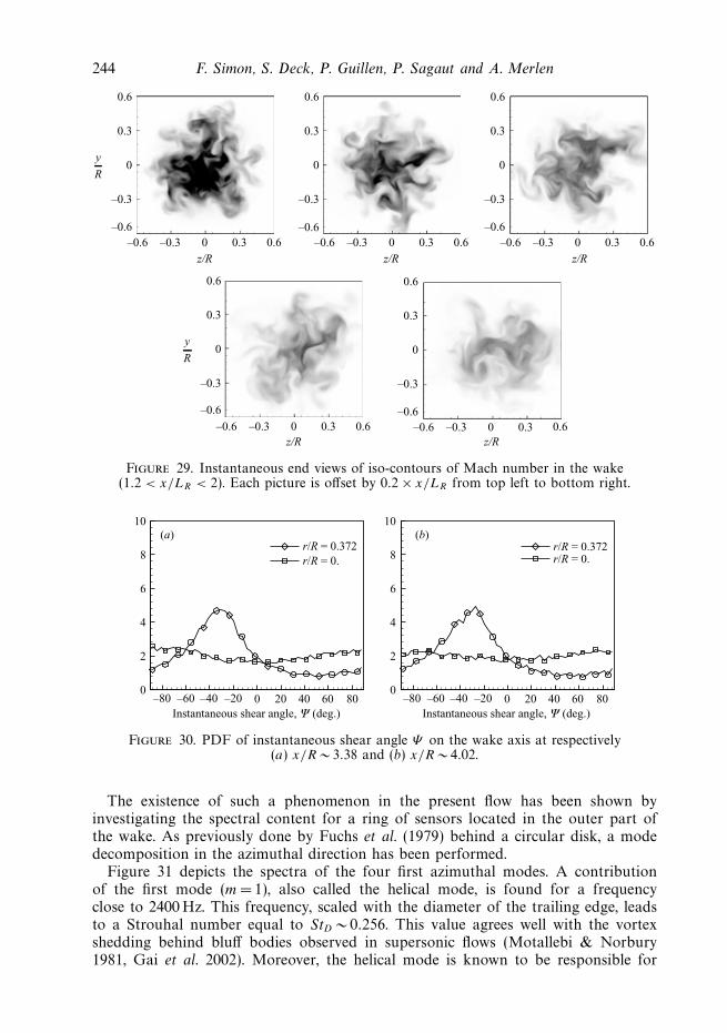
Figure 29. Instantaneous end views of iso-contours of Mach number in the wake(1.2 < x/LR < 2). Each picture is offset by 0.2 × x/LR from top left to bottom right.
Instantaneous shear angle, Ψ (deg.)
r/R = 0.372r/R = 0.r/R = 0.372
r/R = 0.
10
8
6
4
2
0–80 –60 –40 –20 0 20 40 60 80
Instantaneous shear angle, Ψ (deg.)
10
8
6
4
2
0–80 –60 –40 –20 0 20 40 60 80
(a) (b)
Figure 30. PDF of instantaneous shear angle Ψ on the wake axis at respectively(a) x/R ∼ 3.38 and (b) x/R ∼ 4.02.
The existence of such a phenomenon in the present flow has been shown byinvestigating the spectral content for a ring of sensors located in the outer part ofthe wake. As previously done by Fuchs et al. (1979) behind a circular disk, a modedecomposition in the azimuthal direction has been performed.
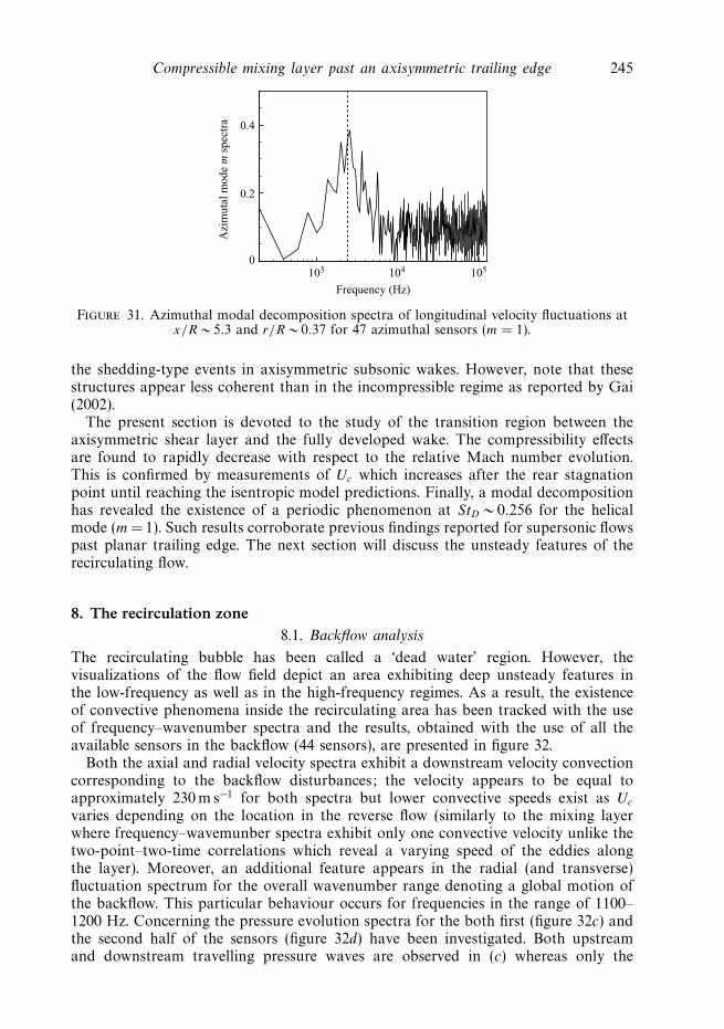
Figure 31 depicts the spectra of the four first azimuthal modes. A contributionof the first mode (m = 1), also called the helical mode, is found for a frequencyclose to 2400 Hz. This frequency, scaled with the diameter of the trailing edge, leadsto a Strouhal number equal to StD ∼ 0.256. This value agrees well with the vortexshedding behind bluff bodies observed in supersonic flows (Motallebi & Norbury1981, Gai et al. 2002). Moreover, the helical mode is known to be responsible for
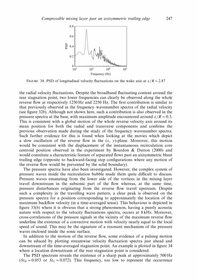
Compressible mixing layer past an axisymmetric trailing edge 245
Azi
mut
al m
ode
m s
pect
ra 0.4
0.2
0103 104
Frequency (Hz)
105
Figure 31. Azimuthal modal decomposition spectra of longitudinal velocity fluctuations atx/R ∼ 5.3 and r/R ∼ 0.37 for 47 azimuthal sensors (m = 1).
the shedding-type events in axisymmetric subsonic wakes. However, note that thesestructures appear less coherent than in the incompressible regime as reported by Gai(2002).
The present section is devoted to the study of the transition region between theaxisymmetric shear layer and the fully developed wake. The compressibility effectsare found to rapidly decrease with respect to the relative Mach number evolution.This is confirmed by measurements of Uc which increases after the rear stagnationpoint until reaching the isentropic model predictions. Finally, a modal decompositionhas revealed the existence of a periodic phenomenon at StD ∼ 0.256 for the helicalmode (m = 1). Such results corroborate previous findings reported for supersonic flowspast planar trailing edge. The next section will discuss the unsteady features of therecirculating flow.
8. The recirculation zone8.1. Backflow analysis
The recirculating bubble has been called a ‘dead water’ region. However, thevisualizations of the flow field depict an area exhibiting deep unsteady features inthe low-frequency as well as in the high-frequency regimes. As a result, the existenceof convective phenomena inside the recirculating area has been tracked with the useof frequency–wavenumber spectra and the results, obtained with the use of all theavailable sensors in the backflow (44 sensors), are presented in figure 32.
Both the axial and radial velocity spectra exhibit a downstream velocity convectioncorresponding to the backflow disturbances; the velocity appears to be equal toapproximately 230 m s−1 for both spectra but lower convective speeds exist as Uc
varies depending on the location in the reverse flow (similarly to the mixing layerwhere frequency–wavemunber spectra exhibit only one convective velocity unlike thetwo-point–two-time correlations which reveal a varying speed of the eddies alongthe layer). Moreover, an additional feature appears in the radial (and transverse)fluctuation spectrum for the overall wavenumber range denoting a global motion ofthe backflow. This particular behaviour occurs for frequencies in the range of 1100–1200 Hz. Concerning the pressure evolution spectra for the both first (figure 32c) andthe second half of the sensors (figure 32d) have been investigated. Both upstreamand downstream travelling pressure waves are observed in (c) whereas only the
246 F. Simon, S. Deck, P. Guillen, P. Sagaut and A. Merlen
Figure 32. Frequency-wavenumber spectra of (a) the longitudinal velocity, (b) and the radialvelocity; and (c) of the pressure first half of the recirculation area and (d) in the second half.
2.5
2.0
1.5
1.0
0.5
1400
1200
1000
800
600
400
200
0102 103 104 105
0 2000 4000
Frequency (Hz)Frequency (Hz)
6000 8000 10000
xR
Gp(
f)*
f(m
s–1
)
(a) (b)
Figure 33. (a) PSD surface of radial velocity fluctuations along the axis in the reverse flowand (b) PSD of pressure fluctuations for the maximum backflow velocity location.
downstream travelling part is clearly visible in (d). The second half of the backflowis dominated by the pressure waves emanating from the vortices of the mixing layerwhich explains the downstream velocity. The upstream waves in (c) represent thepressure disturbances of the reverse flow, as encountered for the velocity spectra. Aparticular phenomena can be observed in figure 32(c) where a spot is clearly visiblein the spectrum around 8000 Hz.
To assess the frequency content of the reverse flow, the spectra of the whole seriesof sensors located on the centreline have also been investigated by the use of PSDsurfaces. An example is plotted in figure 33(a) which addresses the frequency content of
Compressible mixing layer past an axisymmetric trailing edge 247
0.8
0.6
0.4
PS
D
0.2
0102 103
Frequency (Hz)
104 105
Figure 34. PSD of longitudinal velocity fluctuations on the wake axis at x/R ∼ 2.87
the radial velocity fluctuations. Despite the broadband fluctuating content around therear stagnation point, two lower frequencies can clearly be observed along the wholereverse flow at respectively 1250 Hz and 2250 Hz. The first contribution is similar tothat previously observed in the frequency–wavenumber spectra of the radial velocity(see figure 32b). Although not shown here, such a contribution is also observed in thepressure spectra at the base, with maximum amplitude encountered around x/R ∼ 0.5.This is consistent with a global motion of the whole reverse velocity axis around itsmean position for both the radial and transverse components and confirms theprevious observation made during the study of the frequency–wavenumber spectra.Such further evidence for this is found when looking at the movies which depicta slow oscillation of the reverse flow in the (x, y)-plane. Moreover, this motionwould be consistent with the displacement of the instantaneous recirculation corecentroid position observed in the experiment by Bourdon & Dutton (2000) andwould constitute a characteristic feature of separated flows past an axisymmetric blunttrailing edge (opposite to backward-facing step configurations where any motion ofthe reverse flow would be prevented by the solid boundary).
The pressure spectra have also been investigated. However, the complex system ofpressure waves inside the recirculation bubble made them quite difficult to discuss.Pressure waves emanating from the lower side of the vortices in the mixing layertravel downstream in the subsonic part of the flow whereas, at the same time,pressure disturbances originating from the reverse flow travel upstream. Despitesuch a complexity in the travelling wave pattern, a clear peak is observed on thepressure spectra for a position corresponding to approximately the location of themaximum backflow velocity (in a time-averaged sense). This behaviour is depicted infigure 33(b) where it is obvious that a strong phenomenon, having a purely acousticnature with respect to the velocity fluctuations spectra, occurs at 8 kHz. Moreover,cross-correlations of the pressure signals in the vicinity of the maximum reverse flowunderline the existence of a convective motion with velocity nearly equal to the localspeed of sound. This may be the signature of a resonant mechanism of the pressurewaves enclosed inside the sonic surface.
In addition to the motion of the reverse flow, some evidence of a pulsing motioncan be educed by plotting streamwise velocity fluctuation spectra just ahead anddownstream of the time-averaged stagnation point. An example is plotted in figure 34where a location downstream of the rear stagnation point is considered.
The PSD spectrum reveals the existence of a sharp peak at approximately 500 Hz(StD ∼ 0.053 or StL ∼ 0.072). This frequency, too low to represent the occurrence
248 F. Simon, S. Deck, P. Guillen, P. Sagaut and A. Merlen
of convected large-scale structures, may be the signature of a global flow behaviour.Although not shown here, a cross-spectra analysis (between the sensor located nearestto the base and one located at the stagnation point) exhibits coherence level above theonset of coherence required by the method, which corroborates the assumption aboutlarge-scale unsteadiness. The existence of such a similar frequency in both experi-mental (Janssen & Dutton 2004) and numerical pressure spectra at the base centre isfurther evidence of a growing/contracting motion of the whole recirculating flow. Inthe other part of the flow, the spectral signature of this motion may be lost amongstronger fluctuating contributions. It is interesting to note that Shvets (1979) has alsoobserved a low-frequency component in the vicinity of the rear stagnation point in thenear wake of a cone in the supersonic regime, consistent with his experimental visual-izations of a global motion of the whole separated flow behind the base. Evidence ofthe existence of such a low-frequency contribution exists in previous work dealing withseparated flow behind an axisymmetric trailing edge in the subsonic regime. Thus, bothMabey (1972) and Depres (2003) have respectively reported characteristic Strouhalnumbers StD equal to 0.06 and 0.068 at the base centre for axisymmetric base flows.
8.2. Feedback mechanism
As previously mentioned, the recirculating flow area exhibits a very complex physicswhen focusing on its unsteady properties and may be responsible for the existenceof a feedback mechanism triggering the shear layer instability and the self-sustainedoscillations observed in the near wake. Two mechanisms are known to be involved insuch a feedback loop.
The first one concerns oscillations due to the impingement of pressure waves on asolid surface, thus leading to a forcing of the shear layer instability (see the reviewby Rockwell 1983). Such a mechanism may exist in the present flow as the pressurewaves radiating from the coherent vortices on their lower side and those emanatingfrom the reverse flow can be trapped in the subsonic area and can lead to a resonantphenomenon inside the closed sonic surface.
Another mechanism which may be responsible for the appearance of self-sustainedoscillations is the existence of an absolute instability (see Huerre & Monkewitz(1985) for a detailed analysis of convective/absolute instabilities). Monkewitz (1988)has highlighted the absolutely unstable nature of the first helical mode in the nearwake of incompressible axisymmetric bluff bodies for a Reynolds number where self-sustained oscillations are observed. The stability properties of the flow depend uponthe mean local velocity profile. Sevilla & Martinez-Bazan (2004) have demonstratedthat modifying the reverse flow component of the velocity profile can lead to ashift from an absolute to a convective instability of the recirculating flow and thussuppresses the vortex shedding occurring in the near wake. The concept of absoluteinstability has also recently been applied to incompressible backward-facing step flowsby Wee et al. (2004) and to a flow behind a fence by Hudy, Naguib & Humphreys(2003) and Naguib & Hudy (2003). Wee et al. (2004) perform a linear stability analysisto highlight the existence of an absolute instability in the middle of the reverse flowarea with Sth ∼ 0.067 (h is the step height). Hudy et al. (2003) have also observedthe existence of an absolute instability as a source for upstream and downstreamtravelling pressure waves in the recirculating flow. As the absolute nature of the flowmainly depends on the time-averaged velocity profile, such an instability can exist inthe present flow despite its compressible nature, in accordance with the self-sustainedoscillations observed in the developing wake. Very recently, Sandberg & Fasel (2006b)have investigated the transitional base flow at M∞ = 2.46 and have demonstrated the
Compressible mixing layer past an axisymmetric trailing edge 249
existence of an absolute instability for the axisymmetric mode at moderate Reynoldsnumber. This finding makes it highly likely that such an instability exists in thepresent flow and could be related to the large-scale unsteadiness discussed in theprevious section.
Finally, the existence of a secondary vortex structure in the vicinity of the basecorner could play a significant role in the forcing of the shear layer. As in thesimulation of Larcheveque et al. (2004) concerning the compressible flow past acavity, a secondary vortex exists in both the time-averaged and instantaneous flowfields. An animation focusing on this particular part of the flow reveals that the vortexdynamics participates to a certain extent to the generation of large-scale structuresdownstream in the mixing layer during a burst-like phenomenon.
9. ConclusionsA numerical simulation has been carried out of a compressible axisymmetric
shear layer for a Reynolds number near 2.9 × 10⁶. The supersonic free-stream Machnumber before separation involves complex behaviour of the annular mixing layerwith the appearance of several characteristic features. Each part of the flow has beensuccessively discussed in the light of both time-averaged and unsteady data. Thedevelopment of the mixing layer has underlined the strong growth rate of the shearlayer ahead of recompression.
The peak Reynolds stresses increase until the onset of recompression. On enteringthe adverse pressure gradient, the turbulent stresses immediately react to the extrastrain rate, in contrast to its incompressible counterpart. Despite the domination ofthe axial velocity fluctuations, the anisotropy decreases along the shear layer untila constant value of 1.25 is reached, denoting strong changes in the turbulence fieldorganization. Correlation functions have been used to demonstrate the failure ofthe isentropic theory to properly predict the convection velocity of the vortices inthe axisymmetric mixing layer which corroborates previous findings dealing withcanonical planar compressible cases. In the present case, the fast mode dominatesdue to supersonic convective Mach numbers levels. The pressure gradient then leadsto a deceleration of the eddies.
The lateral streamline convergence and the bulk compression involve a complexshock pattern in which the foot shock appears to be constituted by shocks emanatingfrom the upper side of the vortices. Once the fluidic reattachement process isachieved, the compressibility of the flow is quickly damped allowing a recoveryof the incompressible wake behaviour farther downstream. The use of numeroussensors has allowed the characteristics frequencies of the flow to be found, which wasnot possible during the experiment. A wide range of time scales has been highlighted,from the instability process behind the base to the existence of a global motion ofthe separated flow field at very low frequency denoting the very complex unsteadyfeatures of such flows and the difficulties of capturing the whole physics. Thus, furtherevidence of the existence of a flapping motion has been found and the oscillation ofthe reverse flow has been underlined. Finally, an even lower frequency, which may bedue to the motion of the rear stagnation point, has been found.
The authors are greatly indebted to Professors J. C. Dutton, P. Cannon andJ. Forsythe for providing the experimental data. This study is partly funded byGiat Industries within the framework of ONERA/Giat Industries cooperation. R.Cayzac is warmly acknowledged for very stimulating discussions. The authors thank
250 F. Simon, S. Deck, P. Guillen, P. Sagaut and A. Merlen
J. Dandois for fruitful discussions about separated/reattaching flows unsteadinessbehind backward-facing steps.
REFERENCES
Adams, N. A. 2000 Direct simulation of the turbulent boundary layer along a compression rampat M = 3 and Reθ = 1685. J. Fluid Mech. 420, 47–83.
Barre, S., Quine, C. & Dussauge, J. P. 1994 Compressibility effects on the structure of supersonicmixing layers: experimental results. J. Fluid Mech. 259, 47–78.
Baurle, R. A., Tam, C.-J., Edwards, J. R. & Hassan, H. A. 2003 Hybrid simulation approach forcavity flows: blending, algorithm, and boundary treatment issues. AIAA J. 41, 1463–1480.
Bell, J. H. & Mehta, R. D. 1990 Development of a two-stream mixing layer from tripped anduntripped boundary layers. AIAA J. 28, 2034–2042.
Bogdanoff, D. W. 1983 Compressibility effects in turbulent shear layers. AIAA J. 21, 926–927.
Bourdon, C. J. & Dutton, J. C. 1999 Planar visualizations of large-scale turbulent structures inaxisymmetric supersonic flow. AIAA J. 11, 201–213.
Bourdon, C. J. & Dutton, J. C. 2000 Shear layer flapping and interface convolution in a separatedsupersonic flow. AIAA J. 38, 1907–1915.
Bourdon, C. J. & Dutton, J. C. 2001 Effects of boattailing on the turbulence structure of acompressible base flow. J. Spacecraft Rockets 38, 534–541.
Bradshaw, P. 1974 The effect of mean compression or dilatation on the turbulence structure forsupersonic boundary layers. J. Fluid Mech. 63, 449–464.
Breidenthal, R. 1990 The sonic eddy – a model for compressible turbulence. AIAA Paper 90-0495.
Breuer, M., Jocivic, N. & Mazaev, K. 2003 Comparison of DES, RANS and LES for the separatedflow around a flate plate at high incidence. Intl. J. Numer. Meth. Fluids 41, 357–388.
Bunyajitradulya, A. & Papamoschou, D. 1994 Acetone PLIF imaging of turbulent shear-layerstructure at high convective Mach number. AIAA Paper 94-0617.
Cannon, P. M., Elliott, G. S. & Dutton, J. C. 2005 Time-series axisymmetric base-pressuremeasurements with simultaneous near-wake visualizations. AIAA Paper 2005-5285.
Chandrsuda, C. & Bradshaw, P. 1981 Turbulence structure of a reattaching mixing layer. J. FluidMech. 110, 171–194.
Clemens, N. T. & Mungal, M. G. 1995 Large-scale structure and entrainment in the supersonicmixing layer. J. Fluid Mech. 284, 171–216.
Clemens, N. T., Petullo, S. P. & Dolling, D. S. 1996 Large-scale structure evolution in supersonicinteracting shear layers. AIAA J. 34, 2062–2070.
Dandois, J., Garnier, E. & Sagaut, P. 2007 Numerical simulation of active separation control bya synthetic jet. J. Fluid Mech. 574, 25–58.
Deck, S., Garnier, E. & Guillen, P. 2002 Turbulence modelling applied to space launcherconfigurations. J. Turbulence 3, 1–21.
Deck, S., Duveau, P., d’Espiney, P. & Guillen, P. 2002 Development and application ofSpalart Allmaras one equation turbulence model to three-dimensional supersonic complexconfigurations. Aerospace Sci. Tech. 6, 171–183.
Deck, S. 2005a Numerical simulation of transonic buffet over a supercritical airfoil. AIAA J. 43,1556–1566.
Deck, S. 2005b Zonal-detached eddy simulation of the flow around a high-lift configuration. AIAAJ. 43, 2372–2384.
Deck, S. & Thorigny, P. 2007 Unsteadiness of an axisymmetric separating-reattaching flow.Phys. Fluids 19, 065103.
Demetriades, A. 1968 Turbulent front structure of an axisymmetric compressible wake. J. FluidMech. 34, 465–480.
Demetriades, A. 1976 Turbulence correlations in a compressible wake. J. Fluid Mech. 74, 251–267.
Depres, D. 2003 Analyse physique et modelisation des instationnarites dans les ecoulementsd’arriere-corps transsoniques. PhD thesis, University of Aix-Marseille.
Dolling, S. & Murphy, M. T. 1983 Unsteadiness of the separation shock wave structure in asupersonic ramp flowfield. AIAA J. 12, 1628–1634.
Compressible mixing layer past an axisymmetric trailing edge 251
Dolling, S. 2001 Fifty years of shock-wave/boundary-layer interaction research: what next? AIAAJ. 39, 1517–1531.
Elliot, G. S., Samimy, M. & Arnette, S. A. 1995 The characteristics and evolution of large-scalestructures in compressible mixing-layers. Phys. Fluids 7, 864.
Erlebacher, G., Hussaini, M. Y., Speziale, C. G. & Zang, T. A. 1992 Toward the large-eddysimulation of compressible turbulent flows. J. Fluid Mech. 238, 155–185.
Forsythe, J. R., Hoffman, K. A., Cummings, R. M. & Squires, K. D. 2002 Detached-eddysimulation with compressibility corrections applied to a supersonic axisymmetric base flow.J. Fluids Engng. Trans. ASME: 124, 911–923.
Fourguette, D. C., Mungal, M. G. & Dibble, R. W. 1991 Time evolution of the shear layer of asupersonic axisymmetric jet. AIAA J. 29, 1123–1130.
Freund, J. B., Lele, S. K. & Moin, P. 2000 Compressibility effects in a turbulent annular mixinglayer. Part 1. Turbulence and growth rate. J. Fluid Mech. 421, 229–267.
Friedrich, R. & Arnal, M. 1990 Analysing turbulent backward-facing step flow with the lowpass-filtered Navier-Stokes equations. J. Wind Engng Ind. Aerodyn. 35, 101–128.
Fuchs, H. V., Mercker, E. & Michel, U. 1979 Large-scale coherent structures in the wake ofaxisymmetric bodies. J. Fluid Mech. 93, 185–207.
Fureby, C., Nilsson, Y. & Andersson, K. 1999 Large-eddy simulation of supersonic base flow.AIAA Paper 99-0426.
Gai, S. L., Hughes, D. P. & Perry, M. S. 2002 Large-scale structures and growth of a flat platecompressible wake. AIAA J. 40, 1164–1169.
Gaviglio, J., Dussauge, J.-P., Debieve, J.-F. & Favre, A. 1977 Behavior of a turbulent flow, stronglyout of equilibrium, at supersonic speeds. Phys. Fluids 20, 179–192.
Goebel, S. G. & Dutton, J. G. 1990 Experimental study of compressible turbulent mixing layers.AIAA J. 29, 538–546.
Gruber, M. R., Messersmith, N. L. & Dutton, J. G. 1993 Three-dimensional velocity field in acompressible mixing layer. AIAA J. 31, 2061–2067.
Harsha, P. T. & Lee, S. C. 1970 Correlation between turbulent shear stress and turbulent kineticenergy. AIAA J. 8, 1508.
Herrin, J. L. & Dutton, J. C. 1994a Supersonic base flow experiments in the near wake of acylindrical afterbody. AIAA J. 32, 77–83.
Herrin, J. L. & Dutton, J. C. 1994b Supersonic near-wake afterbody boattailing effects onaxisymmetric bodies. J. Spacecraft Rockets 31, 1021–1028.
Herrin, J. L. & Dutton, J. C. 1995 Effect of a rapid expansion on the development of compressiblefree shear layers. Phys. Fluids 7, 159–171.
Herrin, J. L. & Dutton, J. C. 1997 The turbulence structure of a reattaching axisymmetriccompressible free shear layer. Phys. Fluids 9, 3502–3512.
Hudy, L. M., Naguib, A. M. & Humphreys Jr, W. M. 2003 Wall-presure-array measurementsbeneath a separating/reattaching flow region. Phys. Fluids 15, 706–717.
Huerre, P. & Monkewitz, P. A. 1985 Absolute and convective instabilities in free shear layers.J. Fluid Mech. 159, 151–168.
Jackson, T. L. & Grosch, C. E. 1989 Inviscid spatial stability of a compressible mixing layer.J. Fluid Mech. 208, 609–637.
Janssen, J. R. & Dutton, J. C. 2004 Time-series analysis of supersonic basepressure fluctuations.AIAA J. 43, 605–613.
Jeong, J. & Hussain, F. 1995 On the identification of a vortex. J. Fluid Mech. 285, 69–94.
Jovic, S. 1996 An experimental study of a separated/reattached flow behind a backward-facingstep. ReH = 37,000. NASA Tech. Mem. 110384.
Kawai, S. & Fujii, K. 2005 Computational study of supersonic base flow using hybrid turbulencemethodology. AIAA J. 43, 1265–1275.
Larcheveque, L., Sagaut, P., Mary, I., Labbe, O. & Comte, P. 2003 Large-eddy simulation of acompressible flow past a deep cavity. Phys. Fluids 15, 193–210.
Larcheveque, L., Sagaut, P., Le, T.H. & Comte, P. 2004 Large-eddy simulation of a compressibleflow in a three-dimensional open cavity at high Reynolds number. J. Fluid Mech. 516, 265–301.
Mahadevan, R. & Loth, E. 1994 High-speed cinematography of compressible mixing layers.Exps. Fluids 17, 179.
252 F. Simon, S. Deck, P. Guillen, P. Sagaut and A. Merlen
Martens, S., Kimzie, K. W. & McLaughlin, D. K. 1994 Wave structure of coherent instabilitiesin a planar shear layer. AIAA Paper 94-0822.
Mary, I. & Sagaut, P. 2002 Large-eddy simulation of a flow around an airfoil near stall. AIAA J.40, 1139–1145.
Mabey, D. G. 1972 Analysis and correlation of data on pressure fluctuations in separated flow.J. Aircraft 9, 642–645.
Messersmith, N. L. & Dutton, J. C. 1996 Characteristic features of large structures in compressiblemixing layers. AIAA J. 34, 1814–1821.
Monkewitz, P. A. 1988 A note on vortex shedding from axisymmetric bluff bodies. J. Fluid Mech.192, 561–575.
Motallebi, F. & Norbury, J. F. 1981 The effect of base bleed on vortex shedding and base pressurein compressible flow. J. Fluid Mech. 110, 272–292.
Naguib, A. M. & Hudy, L. M. 2003 Stationary and propagating low-frequency wall-pressuredisturbances in a separating/reattaching flow. AIAA Paper 2003-1126.
Olsen, M. G. & Dutton, J. G. 2003 Planar velocity measurements in a weakly compressible mixinglayer. J. Fluid Mech. 486, 51–77.
Pantano, C. & Sarkar, S. 2002 A study of compressibility effects in the highspeed turbulent shearlayer using direct simulation. J. Fluid Mech. 451, 329–371.
Papamoschou, D. & Roshko, A. 1988 The compressible turbulent shear layer: an experimentalstudy. J. Fluid Mech. 197, 453–477.
Papamoschou, D. 1990 Communication paths in the compressible shear layer. AIAA Paper 90-0155.
Papamoschou, D. 1991 Structure of the compressible turbulent shear layer. AIAA J. 29, 680.
Papamoschou, D. & Bunyajitradulya, A. 1995 Double-exposure PLIF imaging of compressibleshear layers. AIAA Paper 95-0531.
Papamoschou, D. & Bunyajitradulya, A. 1997 Evolution of large eddies in compressible shearlayers. Phys. Fluids 9, 756.
Pechier, M., Guillen, P. & Cayzac, R. 2001 Magnus effect over finned projectiles J. SpacecraftRockets 38, 542–549.
Poggie, J. & Smits, A. J. 1996 Large-scale coherent turbulence structures in a compressible mixinglayer flow. AIAA Paper 96-0440.
Poggie, J. & Smits, A. J. 2001 Shock unsteadiness in a reattaching shear layer. J. Fluid Mech. 429,155–185.
Roberts, J. B. 1973 Coherence measurements in an axisymmetric wake. AIAA J. 11, 1569–1571.
Rockwell, D. 1983 Oscillations of impinging shear layers. AIAA J. 21, 645–664.
Sagaut, P., Deck, S. & Terracol, M. 2006 Multiscale and Multiresolution Approaches in Turbulence.Imperial College Press, London, UK.
Samimy, M., Petrie, H. L. & Addy, A. L. 1986 A study of compressible turbulent reattaching freeshear layers. AIAA J. 24, 261–267.
Samimy, M. & Elliot, G. S. 1990 Effects of compressibility on the characteristics of free shearflows. AIAA J. 28, 439–445.
Sandbberg, R. D. & Fasel, H. F. 2006a Direct numerical simulation of transitional supersonicbase flows. AIAA J. 44, 848–858.
Sandberg, R. D. & Fasel, H. F. 2006b Numerical investigation of transitional supersonicaxisymmetric wakes. J. Fluid Mech. 563, 1–41.
Sandham, N. D. & Reynolds, W. C. 1989 Compressible mixing layer: linear theory and directsimulation. AIAA J. 28, 618–624.
Sandham, N. D. & Reynolds, W. C. 1991 Threedimensional simulations of large eddies in thecompressible mixing layer. J. Fluid Mech. 224, 133–158.
Sarkar, S. 1995 The stabilizing effect of compressibility in turbulent shear flow. J. Fluid Mech. 282,163–186.
Sevilla, A. & Martinez-Bazan, C. 2004 Vortex shedding in high Reynolds number axisymmetricbluff-body wakes : Local linear instability and global bleed control. Phys. Fluids 16, 3460–3469.
Shur, M., Spalart, P., Strelets, M. & Travin, A. 1999 Detached-eddy simulation of an airfoilat high angle of attack. 4th Intl. Symp. Engineering Turbulence Modelling and Measurements,pp. 669–678. Elsevier.
Shvets, A. I. 1979 Base pressure fluctuations. Fluid Dyn. 14, 394–401.
Compressible mixing layer past an axisymmetric trailing edge 253
Simon, F., Deck, S., Guillen, P. & Sagaut, P. 2006 RANS/LES simulations of supersonic baseflow. AIAA J. 44, 2578–2590.
Simon, F., Deck, S., Guillen, P., Cayzac, R. & Merlen, A. 2007 Zonal-detached-eddy simulationof projectiles in the subsonic and transonic regimes. AIAA J. 45, 1606–1619.
Simone, A., Coleman, G. N. & Cambon, C. 1997 The effect of compressibility on turbulentshear flow: a rapiddistorsiontheory and directnumericalsimulation study. J. Fluid Mech. 330,307–338.
Smith, K. M. & Dutton, J. C. 1996 Investigation of large-scale structures in supersonic planar baseflows. AIAA J. 34, 1146–1152.
Smith, K. M. & Dutton, J. C. 1999 Evolution and convection of large-scale structures in supersonicreattaching shear flows. Phys. Fluids 11, 2127–2138.
Smith, K. M. & Dutton, J. C. 2001 The effects of expansion strength on large-scale structures incompressible free shear layers. Phys. Fluids 13, 2076–2086.
Spalart, P. R. & Allmaras, S. R. 1992 A one equation turbulence model for aerodynamic flows.AIAA Paper 92-0439.
Spalart, P. R. & Allmaras, S. R. 1994 A one equation turbulence model for aerodynamic flows.La Recherche Aerospatiale, 5–21.
Spalart, P., Jou, W. H., Strelets, M. & Allmaras, S. R. 1997 Comments on the feasibility ofLES for wings and on a hybrid RANS/LES approach. In Proc. 1st AFSOR Int. Conf. onDNS/LES, Ruston.
Spalart, P. R. 2001 Young-person’s guide to detached-eddy simulation grids. NASA/CR-2001-211032.
Spalart, P. R., Deck, S., Shur, M. L., Squires, K. D., Strelets, M. K. & Travin, A. 2006 A newversion of detached-eddy simulation, resistant to ambiguous grid densities. Theor. Comput.Fluid Dyn. 20, 181–195.
Thurow, B., Samimy, M. & Lempert, W. 2003 Compressibility effects on turbulence structures ofaxisymmetric mixing layers. Phys. Fluids 15 (6), 1755–1765.
Urban, W. D. & Mungal, M. G. 2001 Planar velocity measurements in compresible mixing layersJ. Fluid Mech. 431, 189–222.
Vreman, A. W., Sandham, N. D. & Luo, K. H. 1996 Compressible mixing layer growth rate andturbulence characteristics. J. Fluid Mech. 320, 235–258.
Vreman, B., Geurts, B. & Kuerten, H. 1997 Large-eddy simulation of the turbulent mixing layer.J. Fluid Mech. 339, 357–390.
Wee, D., Yi, T., Annaswamy, A. & Ghoniem, A. F. 2004 Self-sustained oscillations and vortexshedding in backward-facing step flows: Simulation and linear instability analysis. Phys. Fluids16, 3361–3373.
Wu, P. P. & Miles, R. B. 2001 Megahertz visualization of compression-corner shock structures.AIAA J. 39, 1542–1546.