NUMERICAL SIMULATION OF THE NONLINEAR SCHR ¨ ODINGER EQUATION WITH MULTI-DIMENSIONAL PERIODIC POTENTIALS ZHONGYI HUANG, SHI JIN, PETER A. MARKOWICH, AND CHRISTOF SPARBER Abstract. By extending the Bloch-decomposition based time-splitting spectral method we intro- duced earlier, we conduct numerical simulations of the dynamics of nonlinear Schr¨ odinger equations subject to periodic and confining potentials. We consider this system as a two-scale asymptotic prob- lem with different scalings of the nonlinearity. In particular we discuss (nonlinear) mass transfer be- tween different Bloch bands and also present three-dimensional simulations for lattice Bose-Einstein condensates in the superfluid regime. version: January 21, 2008 1. Physical motivation Recently there is a growing interest in the theoretical description and the experimental realization of Bose-Einstein condensates (BECs) under the influence of so-called optical lattices, cf. [9, 19, 24, 25]. In such a system there are two extreme situations one needs to distinguish: the superfluid, or Gross- Pitaevskii (GP) regime and the so-called Mott insulator. The two regimes are essentially induced by the strength of the optical lattice, experimentally generated via intense laser fields. In the following we shall focus solely on the superfluid regime, corresponding to situations where the optical lattice potential is of order O(1) in amplitude. The BEC is then usually modelled by the celebrated Gross- Pitaevskii equation, a cubically nonlinear Schr¨ odinger equation (NLS), given by [25] (1.1) i¯ h∂ t ψ = - ¯ h 2 2m Δψ + V (x) ψ + U 0 (x)ψ + Nα|ψ| 2 ψ, x ∈ R 3 ,t ∈ R, where m is the atomic mass, ¯ h is the Planck constant, N is the number of atoms in the condensate and α =4π ¯ h 2 a/m, with a ∈ R denoting the characteristic scattering length of the particles. The external potential U 0 (x) is confining in order to describe the electromagnetic trap needed for the experimental realization of a BEC. Typically it is assumed to be of harmonic form (1.2) U 0 (x)= mω 2 0 |x| 2 2 , ω 0 ∈ R. 2000 Mathematics Subject Classification. 65M70, 74Q10, 35B27, 81Q20. Key words and phrases. nonlinear Schr¨ odinger equation, Bloch decomposition, time-splitting spectral method, Bose- Einstein condensates, Thomas Fermi approximation, lattice potential. This work was partially supported by the Wittgenstein Award 2000 of P. M. and the Austrian-Chinese Technical- Scientific Cooperation Agreement, NSF grant No. DMS-0608720, the NSFC Projects No. 10301017, 10676017 and 10228101, the National Basic Research Program of China under the grant 2005CB321701. C. S. has been supported by the APART grant of the Austrian Academy of Science. P. M. acknowledges support from the Austrian Research Fund FWF through his Wittgenstein Award and from the Wolfson Foundation and the Royal Society through his Royal Society Wolfson Research Merit Award. 1
Transcript
NUMERICAL SIMULATION OF THE NONLINEAR SCHRODINGEREQUATION WITH MULTI-DIMENSIONAL PERIODIC POTENTIALS
ZHONGYI HUANG, SHI JIN, PETER A. MARKOWICH, AND CHRISTOF SPARBER
Abstract. By extending the Bloch-decomposition based time-splitting spectral method we intro-
duced earlier, we conduct numerical simulations of the dynamics of nonlinear Schrodinger equations
subject to periodic and confining potentials. We consider this system as a two-scale asymptotic prob-
lem with different scalings of the nonlinearity. In particular we discuss (nonlinear) mass transfer be-
tween different Bloch bands and also present three-dimensional simulations for lattice Bose-Einstein
condensates in the superfluid regime.
version: January 21, 2008
1. Physical motivation
Recently there is a growing interest in the theoretical description and the experimental realizationof Bose-Einstein condensates (BECs) under the influence of so-called optical lattices, cf. [9, 19, 24, 25].In such a system there are two extreme situations one needs to distinguish: the superfluid, or Gross-Pitaevskii (GP) regime and the so-called Mott insulator. The two regimes are essentially induced bythe strength of the optical lattice, experimentally generated via intense laser fields. In the followingwe shall focus solely on the superfluid regime, corresponding to situations where the optical latticepotential is of order O(1) in amplitude. The BEC is then usually modelled by the celebrated Gross-Pitaevskii equation, a cubically nonlinear Schrodinger equation (NLS), given by [25]
(1.1) ih∂tψ = − h2
2m∆ψ + V (x) ψ + U0(x)ψ + Nα|ψ|2ψ, x ∈ R3, t ∈ R,
where m is the atomic mass, h is the Planck constant, N is the number of atoms in the condensate andα = 4πh2a/m, with a ∈ R denoting the characteristic scattering length of the particles. The externalpotential U0(x) is confining in order to describe the electromagnetic trap needed for the experimentalrealization of a BEC. Typically it is assumed to be of harmonic form
Key words and phrases. nonlinear Schrodinger equation, Bloch decomposition, time-splitting spectral method, Bose-
Einstein condensates, Thomas Fermi approximation, lattice potential.
This work was partially supported by the Wittgenstein Award 2000 of P. M. and the Austrian-Chinese Technical-
Scientific Cooperation Agreement, NSF grant No. DMS-0608720, the NSFC Projects No. 10301017, 10676017 and
10228101, the National Basic Research Program of China under the grant 2005CB321701. C. S. has been supported
by the APART grant of the Austrian Academy of Science. P. M. acknowledges support from the Austrian Research
Fund FWF through his Wittgenstein Award and from the Wolfson Foundation and the Royal Society through his Royal
Society Wolfson Research Merit Award.
1
2 Z. HUANG, S. JIN, P. A. MARKOWICH, AND C. SPARBER
A particular example for the periodic potentials used in physical experiments is then given by [11, 25]
(1.3) V (x) = s3∑
`=1
h2ξ2`
msin2 (ξ`x`) , ξ` ∈ R,
where ξ = (ξ1, ξ2, ξ3) denotes the wave vector of the applied laser field and s > 0 is a dimensionlessparameter describing the depth of the optical lattice (expressed in terms of the recoil energy). TheGP equation (1.1) provides an interesting test case for NLS-codes since it features high frequencyoscillations, two-scale external potentials and a (focusing or defocusing) nonlinearity.
The two-scale nature of the problem is naturally induced by the fact that the external confiningpotential varies slowly (i.e. is almost constant) over a single lattice period. In other words we exhibitmany periods of V on the macroscopic scales induced by the trapping potential. After appropriatescaling, cf. [8, 27], we therefore arrive at the following nonlinear Schodinger equation
(1.4)
iε∂tψε =− ε2
2∆ψε + VΓ
(x
ε
)ψε + U(x)ψε + λε |ψε|2ψε, x ∈ R3,
ψε∣∣t=0
= ψεin(x),
where ε > 0, denotes the semiclassical parameter describing the microscopic/macroscopic scale ratio.The potentials U(x) and VΓ(x/ε) are now given in dimensionless form, such that the two-scale natureof the problem is apparent. The highly oscillating lattice-potential VΓ(y) is assumed to be periodicw.r.t a regular lattice Γ, i.e. VΓ(y + γ) = VΓ(y), for all γ ∈ Γ, y ∈ R3. Here and in what follows, weshall always use the notation y = x/ε for the rescaled spatial variable. The equation (1.4) describesthe motion of the bosons on the macroscopic scale, i.e. ψε = ψε(t, x) is the condensate wave function.It is well known that (1.4) preserves mass
M[ψε(t)
]:=
∫
R3|ψε(t, x)|2dx = M
[ψε
I
],(1.5)
and energy
E[ψε(t)
]:=
∫
R3
(ε2
2|∇ψ(t, x)|2 + (U + VΓ)|ψε(t, x)|2 +
λε
2|ψε(t, x)|4
)dx = E
[ψε
I
],(1.6)
where the first term under the integral is the kinetic energy density, the second is the potential energydensity and the third the nonlinear interaction energy density. In particular we shall be interestedin the semiclassical regime, where ε ¿ 1, allowing for different nonlinearities with different strength.More precisely we will respectively choose λε = O(1) or λε = O(εα), with 0 ≤ α ≤ 1. It is shownin [8, 27], that a particular choice of λε in terms of powers of ε fixes a particular regime of physicalparameters. We remark that, due to the ε-oscillatory nature of solutions of (1.4) the case λε = O(1)corresponds to the regime where dispersion and nonlinear interaction balance dynamically in leadingorder.
In this paper, we extend the one-dimensional Bloch-decomposition based time-splitting spectralmethod developed by the authors in [16] to three-dimensional evolutionary problems of the abovegiven type. We note that earlier numerical studies on closely related problems can be found in[3, 5, 11, 22, 23], relying on different algorithms though. Concisely speaking, the purpose of this paperis threefold:
• Firstly we generalize the numerical method proposed in [16] to a class of physically relevantthree dimensional problems and apply it to case studies of BECs in optical lattices with weak
NONLINEAR SCHRODINGER EQUATION IN PERIODIC POTENTIALS 3
and strong nonlinearities (both, focusing and defocusing). We note that the numerical methodpresented in this work is always based on solving the linear Bloch eigenvalue problem. Howeverwe shall demonstrate that this method works efficiently even in the case where λε = O(1), i.e.the case where dispersion and nonlinearity balance.
• Secondly, we present a comparison to a classical pseudo-spectral method which shows the vastsuperiority of our Bloch-decomposition based approach, particularly in the case of non-smoothpotentials VΓ.
• Thirdly, we study quantitatively the phenomena of mass-transfer between different Blochbands in linear and nonlinear cases. We note that in the latter case, no analytical resultsexist, at least to our knowledge.
The paper is then organized as follows: In section 2, we give a short review of the Bloch decompositionmethod for periodic Schrodinger equations and we also recall the numerical algorithm developed in[16]. We extend the one-dimensional scheme of [16] to three dimensions using operator-splitting. Weconsequently compare our approach with a more standard pseudo-spectral method in Section 3. Insection 4, we first present several numerical tests concerning the (nonlinear) mixing of Bloch bandsbefore we finally show some three-dimensional simulations for lattice BECs as modelled by (1.4).
2. Description of the Bloch-decomposition based numerical method
In this section we will briefly recapitulate the numerical method developed in [16] and discuss itsextension to higher dimensions. For the convenience of the reader we first recall some basic definitionsand important facts to be used when dealing with periodic Schrodinger operators.
2.1. Review of the Bloch decomposition. Let us introduce some notation used throughout thispaper: For the sake of simplicity, set y = x/ε and let the spatial dimension be d = 1 (the extensionto higher dimensions is straightforward). For definiteness, we shall also assume that Γ = 2πZ, i.e.
(2.1) VΓ(y + 2π) = VΓ(y) ∀ y ∈ R.
In this case we have [2]:
• The fundamental domain of our lattice is C = (0, 2π).• The dual lattice Γ∗ is then simply given by Γ∗ = Z.• The fundamental domain of the dual lattice, i.e. the (first) Brillouin zone, is B =
(− 12 , 1
2
).
For our numerical simulations below we shall mainly use the following types of periodic potentials,both of which are well known in the physics literature. Namely, the Mathieu model, i.e.
(2.2) VΓ(x) = cos(x),
and the Kronig-Penney model given by
(2.3) VΓ(x) = 1−∑
γ∈Z1x∈[π
2 +2πγ, 3π2 +2πγ].
4 Z. HUANG, S. JIN, P. A. MARKOWICH, AND C. SPARBER
Next, consider the eigenvalue problem,
(2.4)
(−1
2∂yy + VΓ(y)
)ϕm(y, k) = Em(k)ϕm(y, k),
ϕm(y + 2π, k) = ei2πkyϕm(y, k), ∀ k ∈ B.
It is well known (see [26, 28, 29]) that under very mild conditions on VΓ, the problem (2.4) has acomplete set of eigenfunctions ϕm(y, k),m ∈ N, providing, for each fixed k ∈ B, an orthonormalbasis in L2(C). Correspondingly there exists a countable family of real eigenvalues which can beordered according to E1(k) ≤ E2(k) ≤ · · · ≤ Em(k) ≤ · · · , m ∈ N, taking into account the respectivemultiplicity. The set {Em(k) | k ∈ B} ⊂ R is called the m-th energy band of the operator H. (In thefollowing the index m ∈ N will always denote the band index.)
For convenience we will frequently rewrite ϕm(y, k) as
(2.5) ϕm(y, k) = eikyχm(y, k) ∀m ∈ N,
where now χm(·, k) is 2π-periodic and called Bloch function. In terms of χm(y, k), the eigenvalueproblem (2.4) reads
(2.6)
{H(k)χm(y, k) = Em(k)χm(y, k),
χm(y + 2π, k) = χm(y, k) ∀ k ∈ B,
where
(2.7) H(k) :=12
(−i∂y + k)2 + VΓ(y),
denotes the so-called shifted Hamiltonian. Concerning the dependence on k ∈ B, it has been shown,cf. [26, 29], that for any m ∈ N there exists a closed subset A ⊂ B such that Em(k) is analytic inO = B\A. Similarly, the Bloch functions χm are found to be analytic and periodic in k, for all k ∈ Oand it holds that Em−1(k) < Em(k) < Em+1(k), for all k ∈ O. If this condition is satisfied for allk ∈ B then E`(k) is said to be an isolated Bloch band. Finally we remark that [29]
In this set of measure zero one encounters so-called band crossings. The elements of this set arecharacterized by the fact that Em(k) is only Lipschitz continuous but not differentiable.
By solving the eigenvalue problem (2.4), the Bloch decomposition allows us to decompose theHilbert space H = L2(R) into a direct sum of orthogonal band spaces [21, 26, 29], i.e.
L2(R) =∞⊕
m=1
Hm, Hm :={
fm(y) =∫
Bg(k) ϕm(y, k) dk, g ∈ L2(B)
}.(2.9)
This consequently allows us to write
(2.10) ∀ f ∈ L2(R) : f(y) =∑
m∈Nfm(y), fm ∈ Hm.
The corresponding projection of f onto the m-th band space is given by [21]
fm(y) ≡ (Pmf)(y)
=∫
B
(∫
Rf(ζ)ϕm (ζ, k) dζ
)ϕm (y, k) dk.
(2.11)
NONLINEAR SCHRODINGER EQUATION IN PERIODIC POTENTIALS 5
In what follows, we will denote by
(2.12) Cm(k) :=∫
Rf(ζ)ϕm (ζ, k) dζ
the coefficient of the Bloch decomposition. The main use of the Bloch decomposition is that it reducesan equation of the form
(2.13) i∂tψ = −12
∂yyψ + VΓ(y)ψ, ψ∣∣t=0
= ψin(y),
into countably many, exactly solvable problems on Hm. Indeed in each band space one simply obtains
(2.14) i∂tψm = Em(−i∂y)ψm, ψm
∣∣t=0
= (Pmψin)(y),
where Em(−iε∂y) denotes the Fourier-multiplier corresponding to the symbol Em(k). Using theFourier transformation F , equation (2.14) is easily solved by
(2.15) ψm(t, y) = F−1(e−iEm(k)t(F(Pε
mψin))(k))
.
Here the energy band Em(k) is understood to be periodically extended to all of R.
2.2. The Bloch decomposition based split-step algorithm. In [16] we introduced a new nu-merical method, based on the Bloch decomposition described above. In order to make the paperself-contained, we shall recall here the most important steps of our algorithm and then show how togeneralize it to more than one spatial dimension.
As a necessary preprocessing, we first need to calculate the energy bands Em(k) as well as theeigenfunction ϕm(y, k) from (2.4) (or, likewise from (2.6)). In d = 1 dimension this is rather easyto do and with an acceptable numerical cost as described in [16] (see also [15] for an analogoustreatment). We shall therefore not go into the details here and only remark that the numerical costfor this preprocessing does not depend on the spatial grid to be chosen later on and is therefore almostnegligible when compared to the costs spent in the evolutionary algorithms below.
For the convenience of the computations, we consider the equation (1.4), for d = 1, on a boundeddomain D = [0, 2π] with periodic boundary conditions. This represents an approximation of the(one-dimensional) whole-space problem, as long as the observed wave function does not touch theboundaries x = 0, 2π. Then, for some N ∈ N, t > 0, let the time step be
4t =t
N, and tn = n4t, n = 1, · · · , N.
Suppose that there are L ∈ N lattice cells of Γ within the computational domain D, and that thereare R ∈ N grid points in each lattice cell, which yields the following discretization
(2.16)
k` = − 12
+`− 1
L, where ` = {1, · · · , L} ⊂ N,
yr =2π(r − 1)
R, where r = {1, · · · , R} ⊂ N.
Thus, for any time-step tn, we evaluate ψε(tn, ·), the solution of (1.4), at the grid points
(2.17) x`,r = ε(2π(`− 1) + yr).
Now we introduce the following unitary transformation of f ∈ L2(R)
(2.18) (Tf)(y, k) ≡ f(y, k) :=∑
γ∈Zf(ε(y + 2πγ)) e−i2πkγ , y ∈ C, k ∈ B,
6 Z. HUANG, S. JIN, P. A. MARKOWICH, AND C. SPARBER
such that f(y+2π, k) = e2iπkf(y, k) and f(y, k+1) = f(y, k). In other words f(y, k) admits the sameperiodicity properties w.r.t. k and y as the Bloch eigenfunction ϕm(y, k). Thus we can decomposef(y, k) as a linear combination of such eigenfunctions ϕm(y, k). We introduce the transform T insteadof the traditional Bloch transform, in order to be able to solely use FFT in (2.27) and (2.31) below.Note that the following inversion formula holds
(2.19) f(ε(y + 2πγ)) =∫
Bf(y, k) ei2πkγdk.
Moreover one easily sees that the Bloch coefficient, defined in (2.12), can be equivalently be writtenas
(2.20) Cm(k) =∫
Cf(y, k)ϕm (y, k) dy,
which, in view of (2.5), resembles a Fourier integral.
We are now in position to set up the time-splitting algorithm. To this end, we first set d = 1, forsimplicity. We then solve (1.4) in two steps.
Step 1. First, we solve the equation
(2.21) iε∂tψε = −ε2
2∂xxψε + VΓ
(x
ε
)ψε, x ∈ R,
on a fixed time-interval 4t. To do so we consider for each fixed t ∈ R, the corresponding transformedsolution (Tψε(t, ·)) ≡ ψε(t, y, k), where T is defined in (2.18) and y = x/ε. Note that if we would notuse T here, the solution ψε(t, ·) in general would not satisfy the same periodic boundary conditions(w.r.t. y) as the eigenfunctions ϕm(y, k). After applying T we can decompose ψε(t, y, k) according to
(2.22) ψε(t, y, k) =∑
m∈N(Pmψε) =
∑
m∈NCε
m(t, k)ϕm (y, k) .
Of course, we have to truncate this summation at a certain fixed M ∈ N. Numerical experimentson the band mixing (see also the next section) give us enough experience to choose M large enough,typically M = 32, in order to maintain mass conservation up to a sufficiently high accuracy. By (2.14),this consequently yields the following evolution equation for the coefficient Cε
m(t, k)
(2.23) iε∂tCεm(t, k) = Em(k) Cε
m(t, k),
which yields
(2.24) Cεm(t, k) = Cε
m(0, k)e−iEm(k)t/ε.
Step 2. In the second step, we solve the ordinary differential equation
(2.25) iε∂tψε =
(U(x) + λε|ψε|2
)ψε,
on the same time-interval as before, where the solution obtained in Step 1 serves as initial conditionfor Step 2. Again, we easily obtain the exact solution for this equation by
(2.26) ψε(t, x) = ψε(0, x) e−i(U(x)+λε|ψε|2)t/ε.
Note that this splitting conserves the total particle number ‖ψε(t, x)‖L2 also on the fully discrete leveland is thus unconditionally stable in the sense used by Iserles in [17] (w.r.t. to the discrete L2-norm).Clearly, the algorithm given above is first order in time. But we can easily obtain a second orderscheme by the Strang splitting method, i.e. perform Step 1 with time-step 4t/2, then Step 2 with
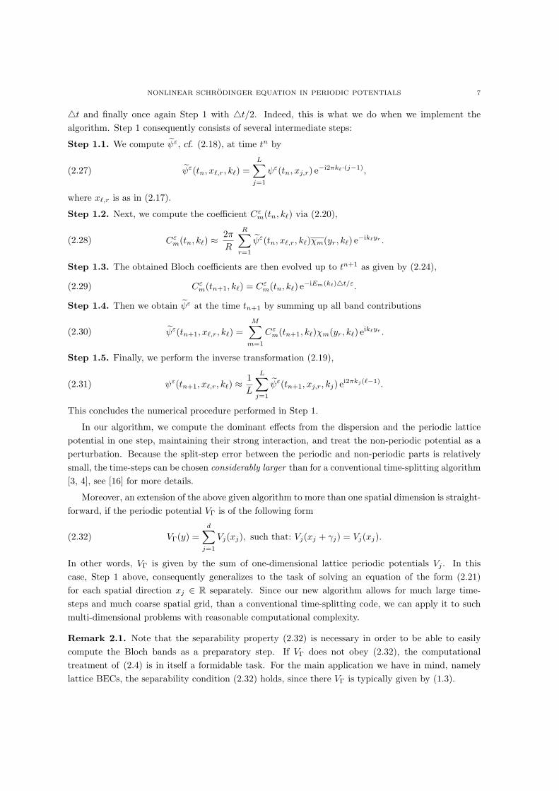
NONLINEAR SCHRODINGER EQUATION IN PERIODIC POTENTIALS 7
4t and finally once again Step 1 with 4t/2. Indeed, this is what we do when we implement thealgorithm. Step 1 consequently consists of several intermediate steps:
Step 1.1. We compute ψε, cf. (2.18), at time tn by
(2.27) ψε(tn, x`,r, k`) =L∑
j=1
ψε(tn, xj,r) e−i2πk`·(j−1),
where x`,r is as in (2.17).
Step 1.2. Next, we compute the coefficient Cεm(tn, k`) via (2.20),
(2.28) Cεm(tn, k`) ≈ 2π
R
R∑r=1
ψε(tn, x`,r, k`)χm(yr, k`) e−ik`yr .
Step 1.3. The obtained Bloch coefficients are then evolved up to tn+1 as given by (2.24),
(2.29) Cεm(tn+1, k`) = Cε
m(tn, k`) e−iEm(k`)4t/ε.
Step 1.4. Then we obtain ψε at the time tn+1 by summing up all band contributions
(2.30) ψε(tn+1, x`,r, k`) =M∑
m=1
Cεm(tn+1, k`)χm(yr, k`) eik`yr .
Step 1.5. Finally, we perform the inverse transformation (2.19),
(2.31) ψε(tn+1, x`,r, k`) ≈ 1L
L∑
j=1
ψε(tn+1, xj,r, kj) ei2πkj(`−1).
This concludes the numerical procedure performed in Step 1.
In our algorithm, we compute the dominant effects from the dispersion and the periodic latticepotential in one step, maintaining their strong interaction, and treat the non-periodic potential as aperturbation. Because the split-step error between the periodic and non-periodic parts is relativelysmall, the time-steps can be chosen considerably larger than for a conventional time-splitting algorithm[3, 4], see [16] for more details.
Moreover, an extension of the above given algorithm to more than one spatial dimension is straight-forward, if the periodic potential VΓ is of the following form
(2.32) VΓ(y) =d∑
j=1
Vj(xj), such that: Vj(xj + γj) = Vj(xj).
In other words, VΓ is given by the sum of one-dimensional lattice periodic potentials Vj . In thiscase, Step 1 above, consequently generalizes to the task of solving an equation of the form (2.21)for each spatial direction xj ∈ R separately. Since our new algorithm allows for much large time-steps and much coarse spatial grid, than a conventional time-splitting code, we can apply it to suchmulti-dimensional problems with reasonable computational complexity.
Remark 2.1. Note that the separability property (2.32) is necessary in order to be able to easilycompute the Bloch bands as a preparatory step. If VΓ does not obey (2.32), the computationaltreatment of (2.4) is in itself a formidable task. For the main application we have in mind, namelylattice BECs, the separability condition (2.32) holds, since there VΓ is typically given by (1.3).
8 Z. HUANG, S. JIN, P. A. MARKOWICH, AND C. SPARBER
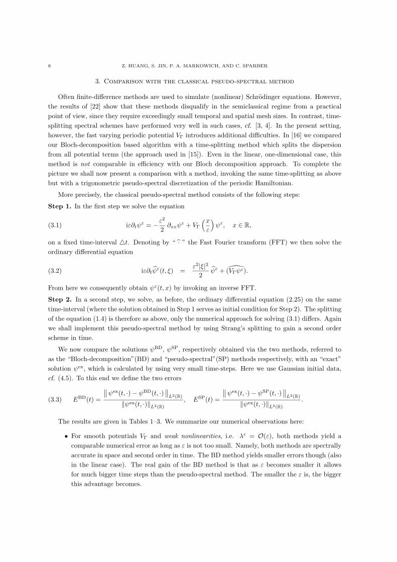
3. Comparison with the classical pseudo-spectral method
Often finite-difference methods are used to simulate (nonlinear) Schrodinger equations. However,the results of [22] show that these methods disqualify in the semiclassical regime from a practicalpoint of view, since they require exceedingly small temporal and spatial mesh sizes. In contrast, time-splitting spectral schemes have performed very well in such cases, cf. [3, 4]. In the present setting,however, the fast varying periodic potential VΓ introduces additional difficulties. In [16] we comparedour Bloch-decomposition based algorithm with a time-splitting method which splits the dispersionfrom all potential terms (the approach used in [15]). Even in the linear, one-dimensional case, thismethod is not comparable in efficiency with our Bloch decomposition approach. To complete thepicture we shall now present a comparison with a method, invoking the same time-splitting as abovebut with a trigonometric pseudo-spectral discretization of the periodic Hamiltonian.
More precisely, the classical pseudo-spectral method consists of the following steps:
Step 1. In the first step we solve the equation
iε∂tψε = −ε2
2∂xxψε + VΓ
(x
ε
)ψε, x ∈ R,(3.1)
on a fixed time-interval 4t. Denoting by “ · ” the Fast Fourier transform (FFT) we then solve theordinary differential equation
iε∂tψε(t, ξ) =
ε2|ξ|22
ψε + (VΓψε).(3.2)
From here we consequently obtain ψε(t, x) by invoking an inverse FFT.
Step 2. In a second step, we solve, as before, the ordinary differential equation (2.25) on the sametime-interval (where the solution obtained in Step 1 serves as initial condition for Step 2). The splittingof the equation (1.4) is therefore as above, only the numerical approach for solving (3.1) differs. Againwe shall implement this pseudo-spectral method by using Strang’s splitting to gain a second orderscheme in time.
We now compare the solutions ψBD, ψSP, respectively obtained via the two methods, referred toas the “Bloch-decomposition”(BD) and “pseudo-spectral”(SP) methods respectively, with an “exact”solution ψex, which is calculated by using very small time-steps. Here we use Gaussian initial data,cf. (4.5). To this end we define the two errors
EBD(t) =
∥∥ψex(t, ·)− ψBD(t, ·) ∥∥L2(R)
‖ψex(t, ·)‖L2(R)
, ESP(t) =
∥∥ψex(t, ·)− ψSP(t, ·)∥∥L2(R)
‖ψex(t, ·)‖L2(R)
.(3.3)
The results are given in Tables 1–3. We summarize our numerical observations here:
• For smooth potentials VΓ and weak nonlinearities, i.e. λε = O(ε), both methods yield acomparable numerical error as long as ε is not too small. Namely, both methods are spectrallyaccurate in space and second order in time. The BD method yields smaller errors though (alsoin the linear case). The real gain of the BD method is that as ε becomes smaller it allowsfor much bigger time steps than the pseudo-spectral method. The smaller the ε is, the biggerthis advantage becomes.
NONLINEAR SCHRODINGER EQUATION IN PERIODIC POTENTIALS 9
−0.5 0 0.5−1
−0.5
0
0.5
1
1.5
2
2.5
3
3.5
m=1
m=1
m=2
m=3
m=4
m=5
m=1
Figure 1. The graph of Em(k) for m = 1, · · · , 5.
• For non-smooth potential VΓ, BD is still spectrally accurate in space and second order in time,while SP is only first order in space and time. The main reason is we can not approximatethe solution with low regularity by trigonometric functions with high accuracy.
• For strong nonlinearities, λε = O(1), and smooth potentials, both methods give comparableresults. Our interpretation for this is that in such cases, the main error comes from thetime-splitting, and the BD does not gain much over the SP.
Our numerical experiments show that, even with the same time-splitting, BD outperforms SP inmany, physically relevant, cases.
4. Numerical Simulations
Before applying our algorithm to the simulation of three-dimensional lattice BECs we shall firststudy in more detail the influence of the nonlinearity on the Bloch decomposition. The correspondingnumerical experiments are of some interest on their own, since so far the mixing of Bloch bands (i.e. themass transfer between different bands) due to nonlinear interactions has not been fully clarified. Weremark that these tests have to seen as mathematical experiments which do not necessarily correspondto realistic physical experiments.
4.1. Numerical experiments on nonlinear band mixing. In this subsection we again restrictourselves to d = 1 spatial dimensions for simplicity. The periodic potential is chosen to be (2.2).Figure 1 shows a plot of the first few energy bands, drawn over B. For the slowly varying, externalpotentials U(x), we shall choose either a simple constant force field, i.e.
(4.1) U(x) = x, x ∈ R,
or a harmonic oscillator type potential (centered in the middle of the computational domain)
(4.2) U(x) =12|x− π|2, x ∈ R.
Obviously, if U(x) 6= 0 an exact treatment along the lines of (2.13) – (2.15) is no longer possible forthe evolution equation (1.4), even if λε = 0. This is due to the fact that one has to take into account
10 Z. HUANG, S. JIN, P. A. MARKOWICH, AND C. SPARBER
Table 1. Comparison tests with U(x) given by (4.2), t = 0.1, VΓ given by (2.2).
λε = 116
, ε = 116
, 4t = 1100000
4x π/32 π/64 π/128 π/256
EBD(t) 2.39E-1 1.86E-3 5.80E-6 2.57E-10
Convergence order 7.0 8.3 14.5
ESP(t) 2.69E-1 3.17E-3 7.64E-6 5.28E-10
Convergence order 6.4 8.7 13.8
λε = 116
, ε = 116
, 4x = π4096
Time step 4t 1/10 1/20 1/40 1/80
EBD(t) 5.95E-2 1.56E-2 3.38E-3 8.69E-4
Convergence order 1.9 2.2 2.0
ESP(t) 1.79E-1 4.49E-2 1.11E-2 2.73E-3
Convergence order 2.0 2.0 2.0
λε = 1128
, ε = 1128
, 4t = 1100000
4x π/256 π/512 π/1024 π/2048
EBD(t) 3.22E-1 2.77E-2 2.81E-5 5.99E-9
Convergence order 3.5 9.9 12.2
ESP(t) 8.85E-1 8.37E-2 2.09E-4 9.44E-8
Convergence order 3.4 8.6 11.1
λε = 1128
, ε = 1128
, 4x = π16384
Time step 4t 1/20 1/40 1/80 1/160
EBD(t) 9.47E-2 2.29E-2 5.23E-3 1.31E-3
Convergence order 2.0 2.0 2.0
Time step 4t 1/200 1/400 1/800 1/1600
ESP(t) 9.67E-2 2.33E-2 5.78E-3 1.45E-3
Convergence order 2.0 2.0 2.0
λε = 0, ε = 11024
, 4t = 1100000
4x π/1024 π/2048 π/4096 π/8192
EBD(t) 9.53E-1 2.88E-1 4.73E-3 1.52E-5
Convergence order 1.7 5.9 8.3
ESP(t) 1.10 5.01E-1 1.92E-2 1.83E-4
Convergence order 1.1 4.7 6.7
λε = 0, ε = 11024
, 4x = π65536
Time step 4t 1/10 1/20 1/40 1/80
EBD(t) 3.50E-2 8.85E-3 2.23E-3 5.59E-4
Convergence order 2.0 2.0 2.0
Time step 4t 1/5000 1/10000 1/20000 1/40000
ESP(t) 7.33E-2 1.83E-2 4.57E-3 1.14E-3
Convergence order 2.0 2.0 2.0
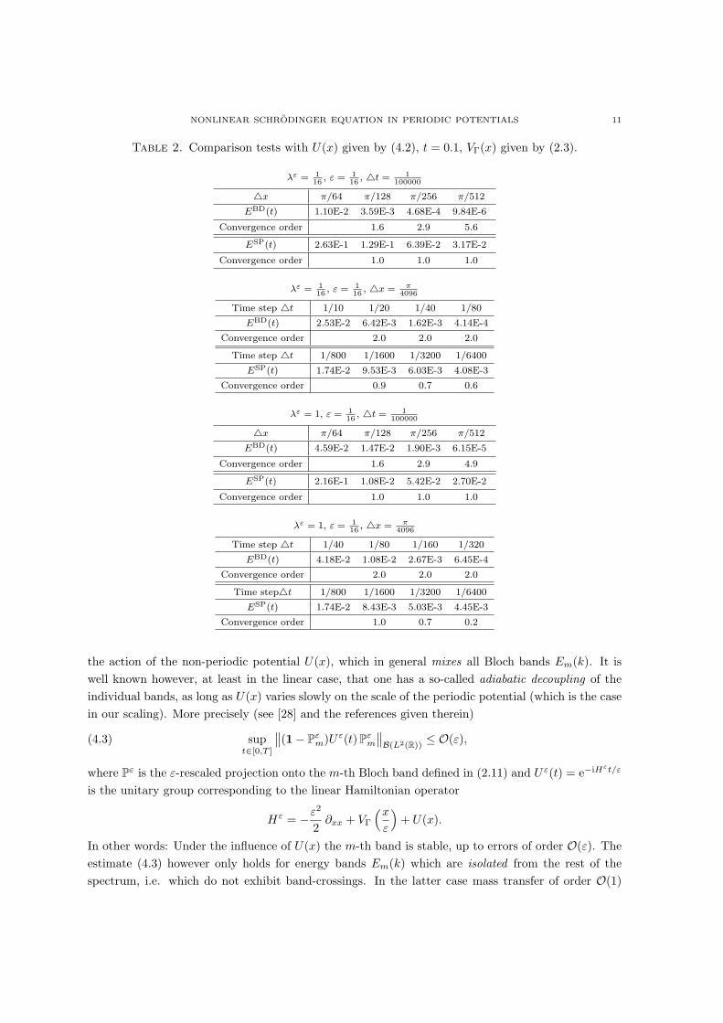
NONLINEAR SCHRODINGER EQUATION IN PERIODIC POTENTIALS 11
Table 2. Comparison tests with U(x) given by (4.2), t = 0.1, VΓ(x) given by (2.3).
λε = 116
, ε = 116
, 4t = 1100000
4x π/64 π/128 π/256 π/512
EBD(t) 1.10E-2 3.59E-3 4.68E-4 9.84E-6
Convergence order 1.6 2.9 5.6
ESP(t) 2.63E-1 1.29E-1 6.39E-2 3.17E-2
Convergence order 1.0 1.0 1.0
λε = 116
, ε = 116
, 4x = π4096
Time step 4t 1/10 1/20 1/40 1/80
EBD(t) 2.53E-2 6.42E-3 1.62E-3 4.14E-4
Convergence order 2.0 2.0 2.0
Time step 4t 1/800 1/1600 1/3200 1/6400
ESP(t) 1.74E-2 9.53E-3 6.03E-3 4.08E-3
Convergence order 0.9 0.7 0.6
λε = 1, ε = 116
, 4t = 1100000
4x π/64 π/128 π/256 π/512
EBD(t) 4.59E-2 1.47E-2 1.90E-3 6.15E-5
Convergence order 1.6 2.9 4.9
ESP(t) 2.16E-1 1.08E-2 5.42E-2 2.70E-2
Convergence order 1.0 1.0 1.0
λε = 1, ε = 116
, 4x = π4096
Time step 4t 1/40 1/80 1/160 1/320
EBD(t) 4.18E-2 1.08E-2 2.67E-3 6.45E-4
Convergence order 2.0 2.0 2.0
Time step4t 1/800 1/1600 1/3200 1/6400
ESP(t) 1.74E-2 8.43E-3 5.03E-3 4.45E-3
Convergence order 1.0 0.7 0.2
the action of the non-periodic potential U(x), which in general mixes all Bloch bands Em(k). It iswell known however, at least in the linear case, that one has a so-called adiabatic decoupling of theindividual bands, as long as U(x) varies slowly on the scale of the periodic potential (which is the casein our scaling). More precisely (see [28] and the references given therein)
(4.3) supt∈[0,T ]
∥∥(1− Pεm)Uε(t)Pε
m
∥∥B(L2(R))
≤ O(ε),
where Pε is the ε-rescaled projection onto the m-th Bloch band defined in (2.11) and Uε(t) = e−iHεt/ε
is the unitary group corresponding to the linear Hamiltonian operator
Hε = −ε2
2∂xx + VΓ
(x
ε
)+ U(x).
In other words: Under the influence of U(x) the m-th band is stable, up to errors of order O(ε). Theestimate (4.3) however only holds for energy bands Em(k) which are isolated from the rest of thespectrum, i.e. which do not exhibit band-crossings. In the latter case mass transfer of order O(1)
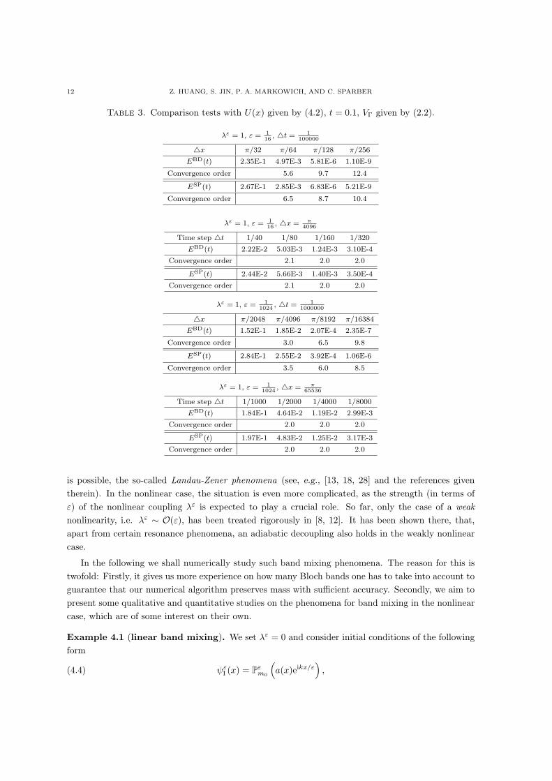
12 Z. HUANG, S. JIN, P. A. MARKOWICH, AND C. SPARBER
Table 3. Comparison tests with U(x) given by (4.2), t = 0.1, VΓ given by (2.2).
λε = 1, ε = 116
, 4t = 1100000
4x π/32 π/64 π/128 π/256
EBD(t) 2.35E-1 4.97E-3 5.81E-6 1.10E-9
Convergence order 5.6 9.7 12.4
ESP(t) 2.67E-1 2.85E-3 6.83E-6 5.21E-9
Convergence order 6.5 8.7 10.4
λε = 1, ε = 116
, 4x = π4096
Time step 4t 1/40 1/80 1/160 1/320
EBD(t) 2.22E-2 5.03E-3 1.24E-3 3.10E-4
Convergence order 2.1 2.0 2.0
ESP(t) 2.44E-2 5.66E-3 1.40E-3 3.50E-4
Convergence order 2.1 2.0 2.0
λε = 1, ε = 11024
, 4t = 11000000
4x π/2048 π/4096 π/8192 π/16384
EBD(t) 1.52E-1 1.85E-2 2.07E-4 2.35E-7
Convergence order 3.0 6.5 9.8
ESP(t) 2.84E-1 2.55E-2 3.92E-4 1.06E-6
Convergence order 3.5 6.0 8.5
λε = 1, ε = 11024
, 4x = π65536
Time step 4t 1/1000 1/2000 1/4000 1/8000
EBD(t) 1.84E-1 4.64E-2 1.19E-2 2.99E-3
Convergence order 2.0 2.0 2.0
ESP(t) 1.97E-1 4.83E-2 1.25E-2 3.17E-3
Convergence order 2.0 2.0 2.0
is possible, the so-called Landau-Zener phenomena (see, e.g., [13, 18, 28] and the references giventherein). In the nonlinear case, the situation is even more complicated, as the strength (in terms ofε) of the nonlinear coupling λε is expected to play a crucial role. So far, only the case of a weaknonlinearity, i.e. λε ∼ O(ε), has been treated rigorously in [8, 12]. It has been shown there, that,apart from certain resonance phenomena, an adiabatic decoupling also holds in the weakly nonlinearcase.
In the following we shall numerically study such band mixing phenomena. The reason for this istwofold: Firstly, it gives us more experience on how many Bloch bands one has to take into account toguarantee that our numerical algorithm preserves mass with sufficient accuracy. Secondly, we aim topresent some qualitative and quantitative studies on the phenomena for band mixing in the nonlinearcase, which are of some interest on their own.
Example 4.1 (linear band mixing). We set λε = 0 and consider initial conditions of the followingform
(4.4) ψεI (x) = Pε
m0
(a(x)eikx/ε
),
NONLINEAR SCHRODINGER EQUATION IN PERIODIC POTENTIALS 13
where, upon setting y = x/ε, the projector Pεm0
is defined (2.11) and the amplitude a(x) ∈ R is givenby a Gaussian
(4.5) a(x) =(
2ω
π
)1/4
e−ω(x−π)2 , ω ∈ R.
We will test the mass transition from the band m0 (for different choices of m0) to other bands, dueto the influence of the potential U(x) given by (4.2). To this end we choose ε = 1/16. We also trieddifferent values for k and ω but there has been no significant difference in our results between thedifferent numerical results. Therefore, we only show the numerical results for ω = 6 and we will chooseeither k = 0 or k = 5 in Fig. 2 and Fig. 3 below. We plot the mass density ρε(t, x) ≡ |ψε(t, x)|2 att = 0 and at the final time t = 1. Clearly, the use of Pε
m0in (4.4) induces high oscillations already in
the initial data. We also show ρεm(t, x) ≡ |Pm(ψε)(t = 1, x)|2, for m = m0, and its corresponding first
few neighboring bands.
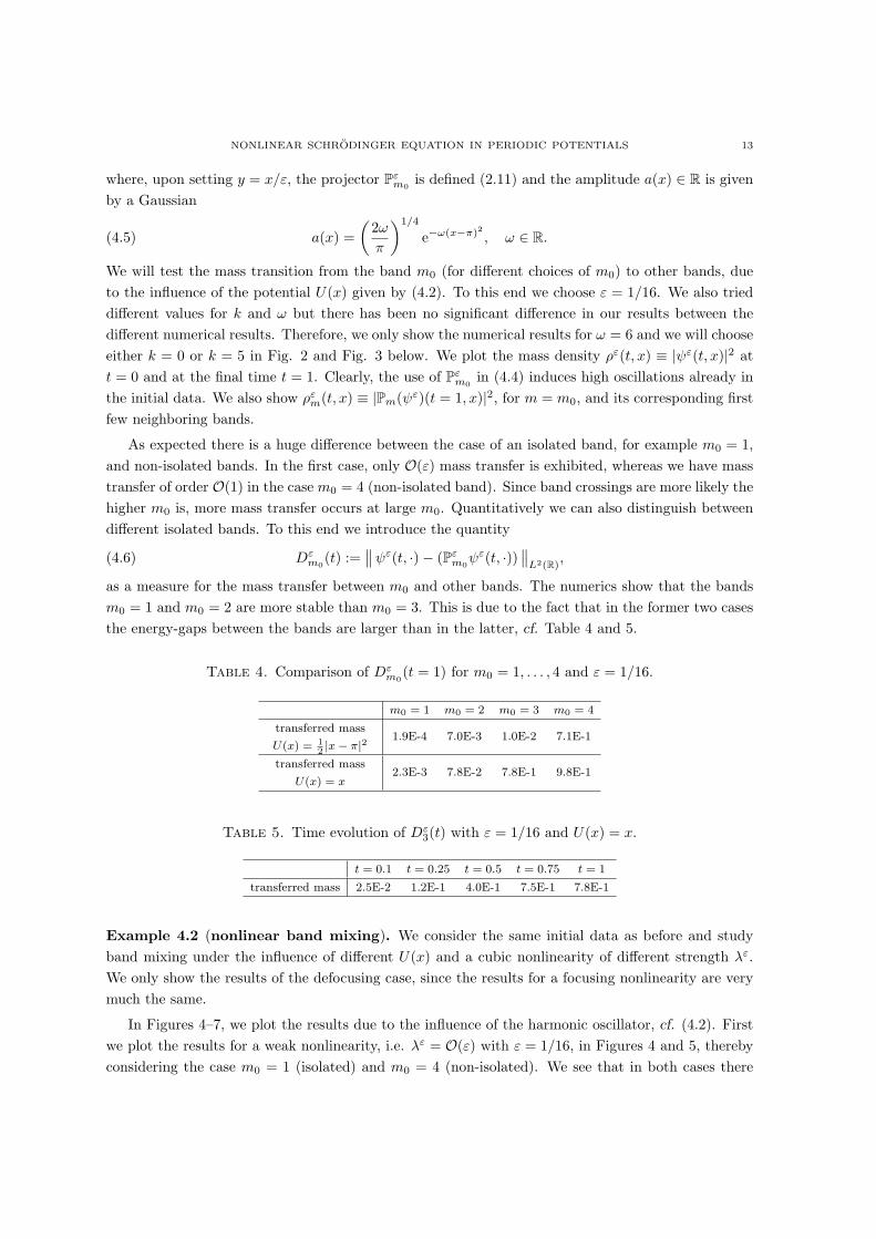
As expected there is a huge difference between the case of an isolated band, for example m0 = 1,and non-isolated bands. In the first case, only O(ε) mass transfer is exhibited, whereas we have masstransfer of order O(1) in the case m0 = 4 (non-isolated band). Since band crossings are more likely thehigher m0 is, more mass transfer occurs at large m0. Quantitatively we can also distinguish betweendifferent isolated bands. To this end we introduce the quantity
(4.6) Dεm0
(t) :=∥∥ψε(t, ·)− (Pε
m0ψε(t, ·))
∥∥L2(R)
,
as a measure for the mass transfer between m0 and other bands. The numerics show that the bandsm0 = 1 and m0 = 2 are more stable than m0 = 3. This is due to the fact that in the former two casesthe energy-gaps between the bands are larger than in the latter, cf. Table 4 and 5.
Table 4. Comparison of Dεm0
(t = 1) for m0 = 1, . . . , 4 and ε = 1/16.
m0 = 1 m0 = 2 m0 = 3 m0 = 4
transferred mass
U(x) = 12|x− π|2 1.9E-4 7.0E-3 1.0E-2 7.1E-1
transferred mass
U(x) = x2.3E-3 7.8E-2 7.8E-1 9.8E-1
Table 5. Time evolution of Dε3(t) with ε = 1/16 and U(x) = x.
t = 0.1 t = 0.25 t = 0.5 t = 0.75 t = 1
transferred mass 2.5E-2 1.2E-1 4.0E-1 7.5E-1 7.8E-1
Example 4.2 (nonlinear band mixing). We consider the same initial data as before and studyband mixing under the influence of different U(x) and a cubic nonlinearity of different strength λε.We only show the results of the defocusing case, since the results for a focusing nonlinearity are verymuch the same.
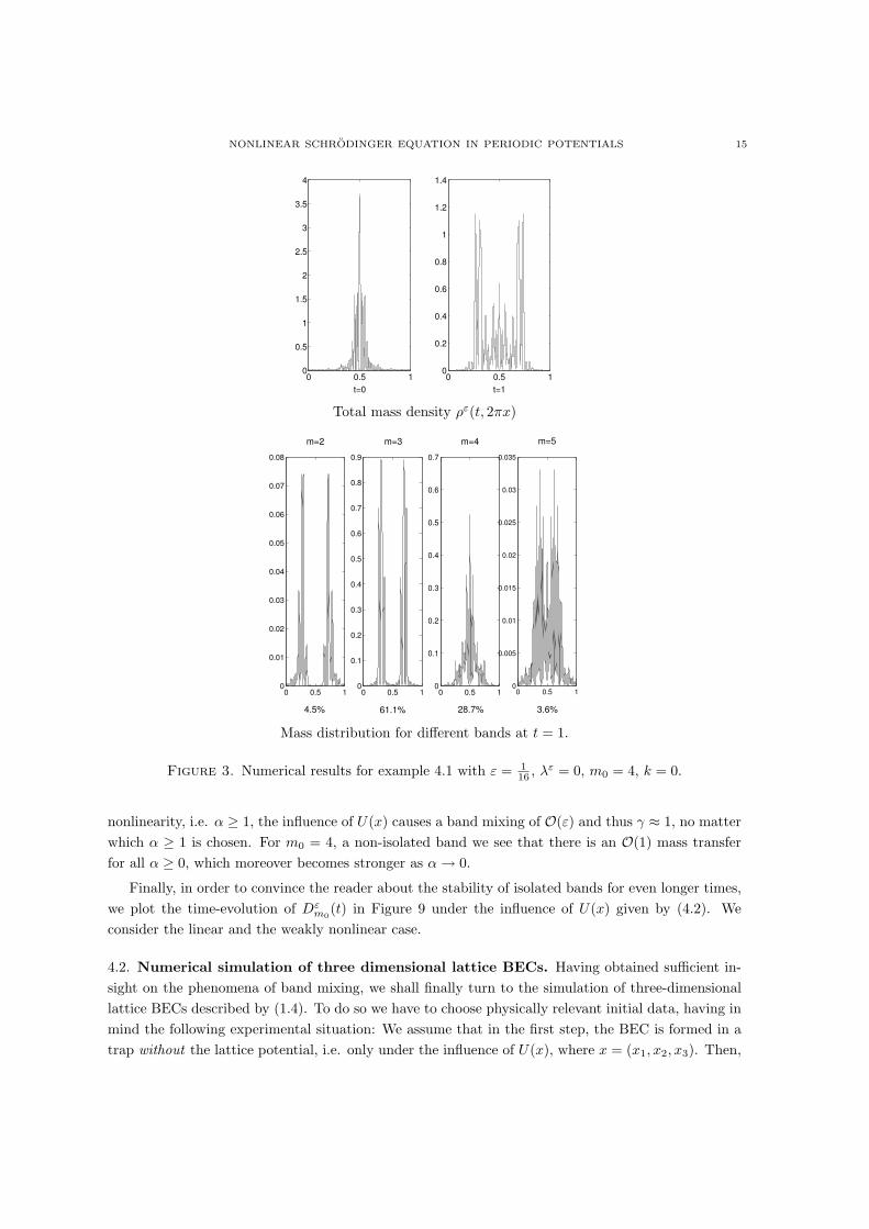
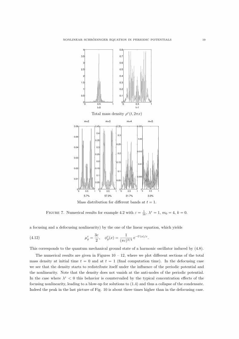
In Figures 4–7, we plot the results due to the influence of the harmonic oscillator, cf. (4.2). Firstwe plot the results for a weak nonlinearity, i.e. λε = O(ε) with ε = 1/16, in Figures 4 and 5, therebyconsidering the case m0 = 1 (isolated) and m0 = 4 (non-isolated). We see that in both cases there
14 Z. HUANG, S. JIN, P. A. MARKOWICH, AND C. SPARBER
0.3 0.4 0.5 0.6 0.70
0.5
1
1.5
2
2.5
3
3.5
4
4.5
t=00.3 0.4 0.5 0.6 0.70
0.5
1
1.5
2
2.5
3
3.5
4
4.5
t=1
Total mass density ρε(t, 2πx)
0 0.5 10
0.5
1
1.5
2
2.5
3
3.5
4
4.5
m=1
99.97%
0 0.5 10
0.2
0.4
0.6
0.8
1x 10
−3m=2
0.03%
0 0.5 10
0.2
0.4
0.6
0.8
1
1.2x 10
−5m=3
0 0.5 10
0.5
1
1.5
2
2.5
3x 10
−7m=4
Mass distribution for different bands at t = 1.
Figure 2. Numerical results for example 4.1 with ε = 116 , λε = 0, m0 = 1, k = 5.
is no significant difference in comparison with the linear situation. This changes dramatically thoughwhen we choose λε = O(1), see Figures 6 and 7. For such a strong nonlinearity, the mass transfer isO(1), even in the case of an isolated band, i.e. m0 = 1.
To get a more detailed picture of the influence of a cubic nonlinearity we consider, for any fixedt∗ ∈ R of order O(1),
(4.7) λε = O(εα), Dεm0
(t∗) = O(εγ), α, γ ≥ 0,
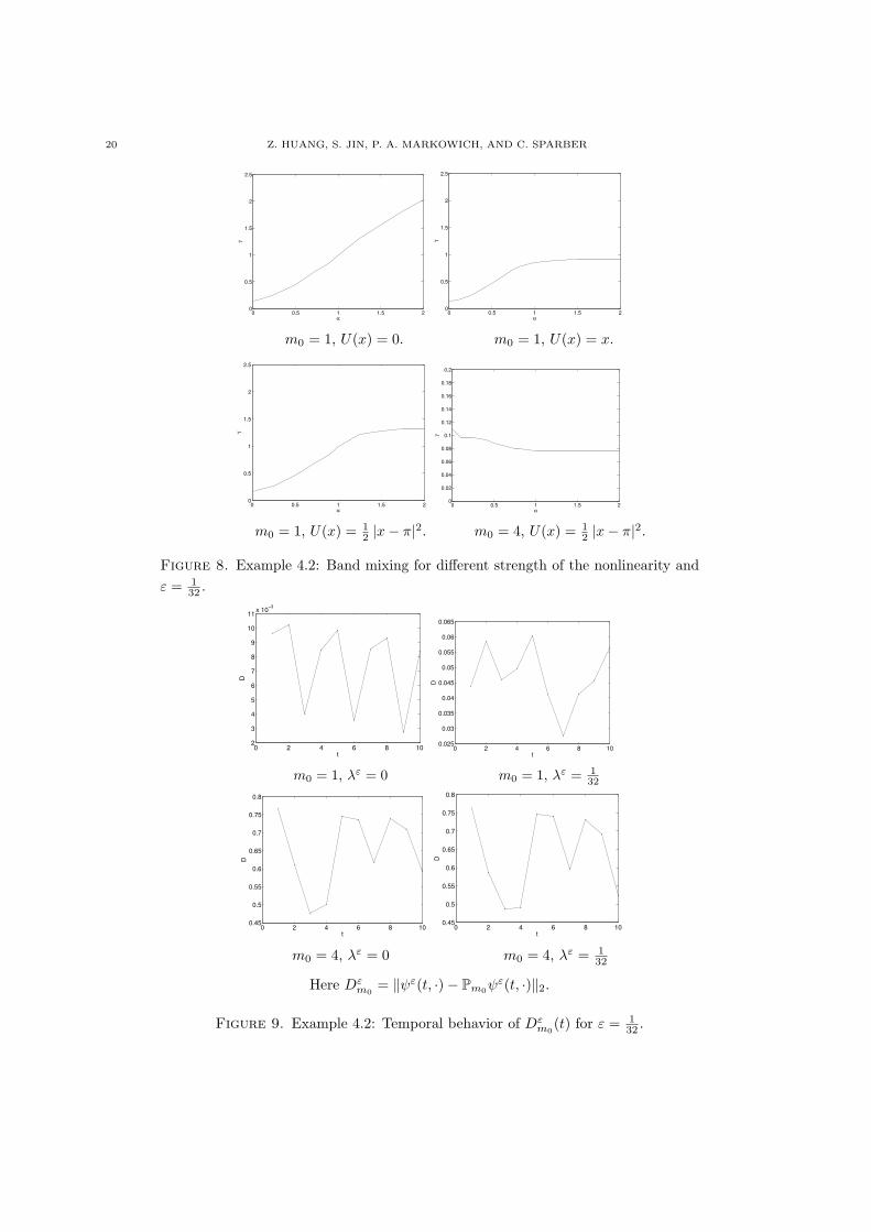
and we aim to numerically quantify the connection between α and γ. The results for different U(x)and m0 = 1, or m0 = 4 are shown in Figure 8, which is plotted for t∗ = 1 and ε = 1/32:
First we consider the isolated band m0 = 1: We see that in the case of vanishing external potentials,i.e. U(x) = 0 we have α ≈ γ. The same holds true for a non-zero U(x) and 0 ≤ α ≤ 1, the regime inwhich the nonlinearity is (formally) stronger as the external potential. However, for an even smaller
NONLINEAR SCHRODINGER EQUATION IN PERIODIC POTENTIALS 15
0 0.5 10
0.5
1
1.5
2
2.5
3
3.5
4
t=00 0.5 1
0
0.2
0.4
0.6
0.8
1
1.2
1.4
t=1
Total mass density ρε(t, 2πx)
0 0.5 10
0.01
0.02
0.03
0.04
0.05
0.06
0.07
0.08
m=2
4.5%
0 0.5 10
0.1
0.2
0.3
0.4
0.5
0.6
0.7
0.8
0.9
m=3
61.1%
0 0.5 10
0.1
0.2
0.3
0.4
0.5
0.6
0.7
m=4
28.7%
0 0.5 10
0.005
0.01
0.015
0.02
0.025
0.03
0.035
m=5
3.6%
Mass distribution for different bands at t = 1.
Figure 3. Numerical results for example 4.1 with ε = 116 , λε = 0, m0 = 4, k = 0.
nonlinearity, i.e. α ≥ 1, the influence of U(x) causes a band mixing of O(ε) and thus γ ≈ 1, no matterwhich α ≥ 1 is chosen. For m0 = 4, a non-isolated band we see that there is an O(1) mass transferfor all α ≥ 0, which moreover becomes stronger as α → 0.
Finally, in order to convince the reader about the stability of isolated bands for even longer times,we plot the time-evolution of Dε
m0(t) in Figure 9 under the influence of U(x) given by (4.2). We
consider the linear and the weakly nonlinear case.
4.2. Numerical simulation of three dimensional lattice BECs. Having obtained sufficient in-sight on the phenomena of band mixing, we shall finally turn to the simulation of three-dimensionallattice BECs described by (1.4). To do so we have to choose physically relevant initial data, having inmind the following experimental situation: We assume that in the first step, the BEC is formed in atrap without the lattice potential, i.e. only under the influence of U(x), where x = (x1, x2, x3). Then,
16 Z. HUANG, S. JIN, P. A. MARKOWICH, AND C. SPARBER
0.3 0.4 0.5 0.6 0.70
0.5
1
1.5
2
2.5
3
3.5
4
4.5
t=00.3 0.4 0.5 0.6 0.70
0.5
1
1.5
2
2.5
3
3.5
4
4.5
t=1
Total mass density ρε(t, 2πx)
0 0.5 10
0.5
1
1.5
2
2.5
3
3.5
4
4.5
m=1
99.58%
0 0.5 10
0.5
1
1.5
2
2.5
3x 10
−4m=2
0.01%
0 0.5 10
1
2
3
4
5
6
7
8x 10
−3m=3
0.38%
0 0.5 10
0.5
1
1.5
2
2.5
3
3.5
4
4.5x 10
−4m=4
0.03%
Mass distribution for different bands at t = 1.
Figure 4. Numerical results for example 4.2 with ε = 116 , λε = 1
16 , m0 = 1, k = 5.
in a second step, we assume that the lattice potential VΓ(x/ε) is switched on and the (nonlinear)dynamics of the BEC under the combined influence of U(x) and VΓ(x/ε) is studied. For definitenesswe shall from now on consider the following potentials acting on the BEC
(4.8) VΓ (x) =3∑
`=1
sin2 (x`) , U(x) =12
3∑
`=1
|x` − π|2.
These choices, obtained from the potentials (1.2)–(1.3) by scaling, are consistent with various physicalexperiments [1, 6, 9, 10, 19, 25].
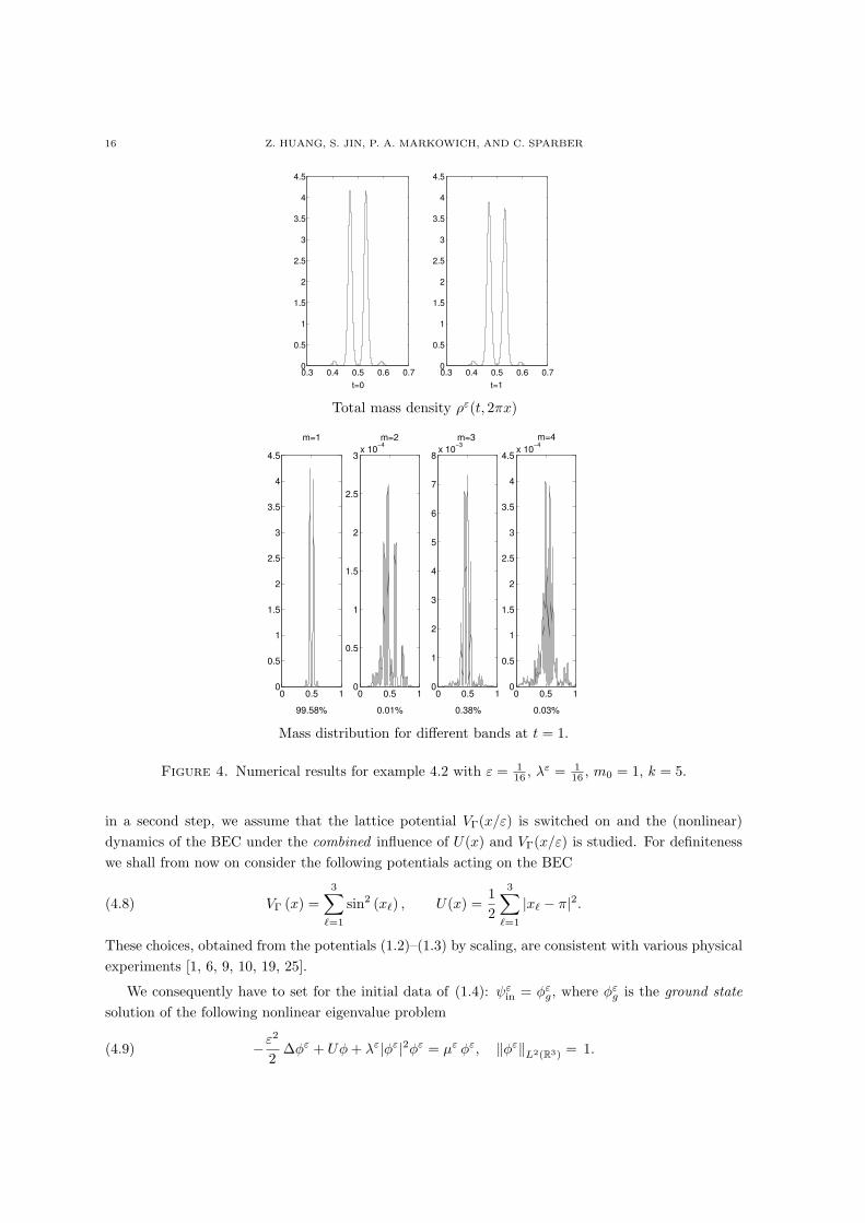
We consequently have to set for the initial data of (1.4): ψεin = φε
g, where φεg is the ground state
solution of the following nonlinear eigenvalue problem
(4.9) −ε2
2∆φε + Uφ + λε|φε|2φε = µε φε, ‖φε‖L2(R3) = 1.
NONLINEAR SCHRODINGER EQUATION IN PERIODIC POTENTIALS 17
0 0.5 10
0.5
1
1.5
2
2.5
3
3.5
4
t=00 0.5 1
0
0.2
0.4
0.6
0.8
1
1.2
1.4
t=1
Total mass density ρε(t, 2πx)
0 0.5 10
0.01
0.02
0.03
0.04
0.05
0.06
0.07
m=2
4.2%
0 0.5 10
0.1
0.2
0.3
0.4
0.5
0.6
0.7
0.8
0.9
1
m=3
61.8%
0 0.5 10
0.1
0.2
0.3
0.4
0.5
0.6
0.7
m=4
28.4%
0 0.5 10
0.005
0.01
0.015
0.02
0.025
0.03
0.035
m=5
3.6%
Mass distribution for different bands at t = 1.
Figure 5. Numerical results for example 4.2 with ε = 116 , λε = 1
16 , m0 = 4, k = 0.
The ground state may be characterized as the unique (non-negative) solution φε = φεg of (4.9) with
corresponding minimal chemical potential µε ∈ R. For a repulsive, or defocusing nonlinearity, i.e.λε > 0, the ground state can the obtained by minimizing the energy E
[φε
], in (1.6) with VΓ ≡ 0,
under the constraint ‖φε‖L2(R3) = 1 (see [20] for more details). For an attractive or focusing three-dimensional condensate a global minimizer of E[φε] does not exist. Also, the interpretation of criticalpoints of the energy functional as possible candidates for the corresponding physical ground stateis not clear. Note however, that there are recent experiments [1, 10] where one is able to tune thenonlinear interaction λε = λε(t) from positive into negative by using so-called Feshbach resonances.Thus, also the case of a focusing nonlinearity in (1.4) is of physical interest.
18 Z. HUANG, S. JIN, P. A. MARKOWICH, AND C. SPARBER
0 0.5 10
0.5
1
1.5
2
2.5
3
3.5
4
4.5
t=0
0 0.5 10
0.2
0.4
0.6
0.8
1
1.2
1.4
1.6
1.8
t=1
Total mass density ρε(t, 2πx)
0 0.5 10
0.5
1
1.5
2
2.5
3
m=1
68.9%
0 0.5 10
0.002
0.004
0.006
0.008
0.01
0.012
0.014
m=2
1.1%
0 0.5 10
0.05
0.1
0.15
0.2
0.25
0.3
0.35
m=3
18.2%
0 0.5 10
0.01
0.02
0.03
0.04
0.05
0.06
0.07
m=4
9.9%
Mass distribution for different bands at t = 1.
Figure 6. Numerical results for example 4.2 with ε = 116 , λε = 1, m0 = 1, k = 0.
Example 4.3 (3d lattice BEC, weak nonlinearity). We study the weakly nonlinear situationwhere λε = O(ε). Following the scaling given in [8], we find that in this case
(4.10) ε =(
a0
4πN |a|)2/3
.
For example, in the case of a lattice BEC consisting of Rb atoms we have, cf. [11]:
(4.11) a0 ≈ 3, 4× 10⁻⁶[m], a ≈ 5, 4× 10⁻⁹[m].
The following numerical simulations are done for ε = 1/4, which corresponds to N ≈ 500 atoms inthe optical lattice of the form (1.3), where s = 1 and ξl ≈ 4, 6× 10⁶[1/m]. Clearly, bigger values of N
correspond to smaller values of ε which leads to longer running-times of the code. Since λε = O(ε),the ground state of the nonlinear eigenvalue problem (4.9) can be very well approximated (for, both,
NONLINEAR SCHRODINGER EQUATION IN PERIODIC POTENTIALS 19
0 0.5 10
0.5
1
1.5
2
2.5
3
3.5
4
t=00 0.5 1
0
0.1
0.2
0.3
0.4
0.5
0.6
0.7
0.8
t=1
Total mass density ρε(t, 2πx)
0 0.5 10
0.01
0.02
0.03
0.04
0.05
0.06
m=2
5.7%
0 0.5 10
0.05
0.1
0.15
0.2
0.25
0.3
0.35
0.4
0.45
m=3
57.0%
0 0.5 10
0.05
0.1
0.15
0.2
0.25
0.3
0.35
m=4
31.7%
0 0.5 10
0.005
0.01
0.015
0.02
0.025
m=5
3.0%
Mass distribution for different bands at t = 1.
Figure 7. Numerical results for example 4.2 with ε = 116 , λε = 1, m0 = 4, k = 0.
a focusing and a defocusing nonlinearity) by the one of the linear equation, which yields
(4.12) µεg =
3ε
2, φε
g(x) =1
(πε)3/4e−U(x)/ε.
This corresponds to the quantum mechanical ground state of a harmonic oscillator induced by (4.8).
The numerical results are given in Figures 10 – 12, where we plot different sections of the totalmass density at initial time t = 0 and at t = 1 (final computation time). In the defocusing casewe see that the density starts to redistribute itself under the influence of the periodic potential andthe nonlinearity. Note that the density does not vanish at the anti-nodes of the periodic potential.In the case where λε < 0 this behavior is countervailed by the typical concentration effects of thefocusing nonlinearity, leading to a blow-up for solutions to (1.4) and thus a collapse of the condensate.Indeed the peak in the last picture of Fig. 10 is about three times higher than in the defocusing case.
20 Z. HUANG, S. JIN, P. A. MARKOWICH, AND C. SPARBER
0 0.5 1 1.5 20
0.5
1
1.5
2
2.5
α
γ
0 0.5 1 1.5 20
0.5
1
1.5
2
2.5
α
γ
m0 = 1, U(x) = 0. m0 = 1, U(x) = x.
0 0.5 1 1.5 20
0.5
1
1.5
2
2.5
α
γ
0 0.5 1 1.5 20
0.02
0.04
0.06
0.08
0.1
0.12
0.14
0.16
0.18
0.2
α
γ
m0 = 1, U(x) = 12 |x− π|2. m0 = 4, U(x) = 1
2 |x− π|2.
Figure 8. Example 4.2: Band mixing for different strength of the nonlinearity andε = 1
32 .
0 2 4 6 8 102
3
4
5
6
7
8
9
10
11x 10
−3
t
D
0 2 4 6 8 100.025
0.03
0.035
0.04
0.045
0.05
0.055
0.06
0.065
t
D
m0 = 1, λε = 0 m0 = 1, λε = 132
0 2 4 6 8 100.45
0.5
0.55
0.6
0.65
0.7
0.75
0.8
t
D
0 2 4 6 8 100.45
0.5
0.55
0.6
0.65
0.7
0.75
0.8
t
D
m0 = 4, λε = 0 m0 = 4, λε = 132
Here Dεm0
= ‖ψε(t, ·)− Pm0ψε(t, ·)‖2.
Figure 9. Example 4.2: Temporal behavior of Dεm0
(t) for ε = 132 .
NONLINEAR SCHRODINGER EQUATION IN PERIODIC POTENTIALS 21
ρε(t = 0, 2πx)∣∣x3=0
(initial density), ρε+(t = 1, 2πx)
∣∣x3=0
(defocusing case) andρε−(t = 1, 2πx)
∣∣x3=0
(focusing case).
Figure 10. Example 4.3 (weak nonlinearity): Comparison of the initial and finalmass densities, evaluated at x3 = 0, with |λε| = 1
4 and ε = 14 .
Figure 11. Example 4.3 (weak nonlinearity, defocusing case): Surface plot of|ψε(t, 2πx)| = 0.25 at different times with λε = 1
4 and ε = 14 .
However, due to the asymptotic smallness of the nonlinearity it might still be possible to obtain a(stable) periodic condensate over the life-time of the experiment.
22 Z. HUANG, S. JIN, P. A. MARKOWICH, AND C. SPARBER
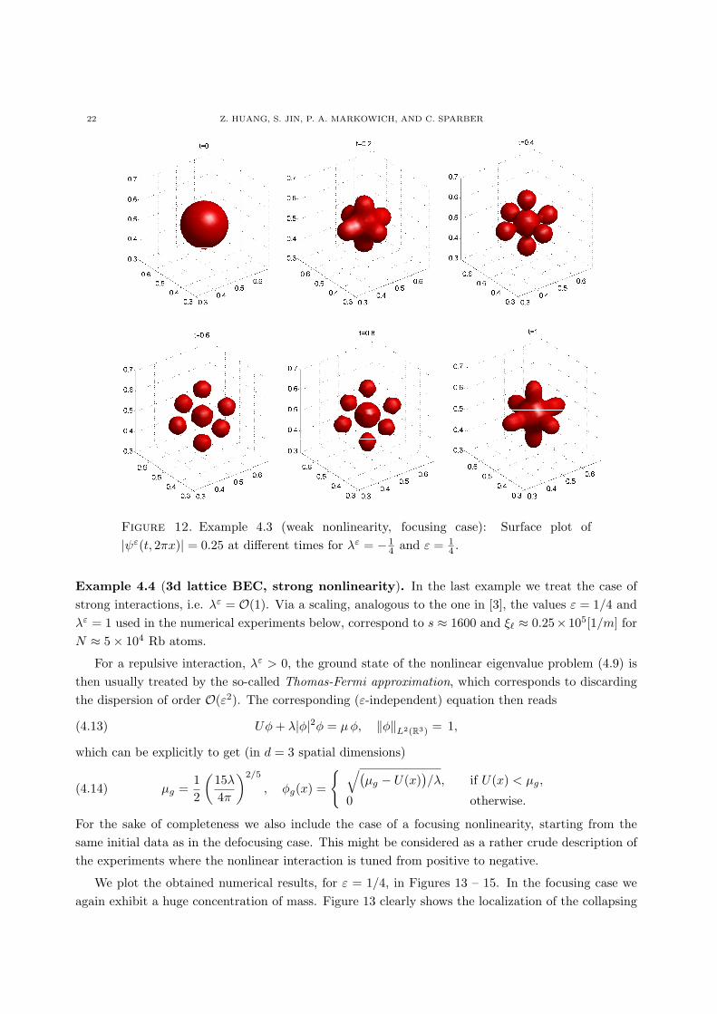
Figure 12. Example 4.3 (weak nonlinearity, focusing case): Surface plot of|ψε(t, 2πx)| = 0.25 at different times for λε = − 1
4 and ε = 14 .
Example 4.4 (3d lattice BEC, strong nonlinearity). In the last example we treat the case ofstrong interactions, i.e. λε = O(1). Via a scaling, analogous to the one in [3], the values ε = 1/4 andλε = 1 used in the numerical experiments below, correspond to s ≈ 1600 and ξ` ≈ 0.25× 10⁵[1/m] forN ≈ 5× 10⁴ Rb atoms.
For a repulsive interaction, λε > 0, the ground state of the nonlinear eigenvalue problem (4.9) isthen usually treated by the so-called Thomas-Fermi approximation, which corresponds to discardingthe dispersion of order O(ε2). The corresponding (ε-independent) equation then reads
(4.13) Uφ + λ|φ|2φ = µφ, ‖φ‖L2(R3) = 1,
which can be explicitly to get (in d = 3 spatial dimensions)
(4.14) µg =12
(15λ
4π
)2/5
, φg(x) =
{ √(µg − U(x)
)/λ, if U(x) < µg,
0 otherwise.
For the sake of completeness we also include the case of a focusing nonlinearity, starting from thesame initial data as in the defocusing case. This might be considered as a rather crude description ofthe experiments where the nonlinear interaction is tuned from positive to negative.
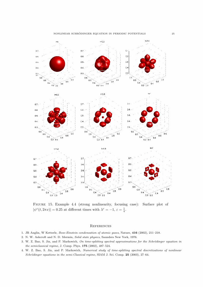
We plot the obtained numerical results, for ε = 1/4, in Figures 13 – 15. In the focusing case weagain exhibit a huge concentration of mass. Figure 13 clearly shows the localization of the collapsing
NONLINEAR SCHRODINGER EQUATION IN PERIODIC POTENTIALS 23
ρε(t = 0, 2πx)∣∣x3=0
(initial density), ρε+(t = 1, 2πx)
∣∣x3=0
(defocusing case) and ρε−(t = 1, 2πx)
∣∣x3=0
(focusing case).
ρε+(t = 2, 2πx)
∣∣x3=0
(defocusing case) and ρε−(t = 2, 2πx)
∣∣x3=0
(focusing case).
Figure 13. Example 4.4 (strong nonlinearity): Comparison of the initial and finalmass densities, evaluated at x3 = 0, with |λε| = 1 and ε = 1
4 .
solution, invoking large gradients, i.e. sharp peaks. Note that during the course of time several largepeaks occur which eventually combine to one. Moreover we clearly see that due to the influence ofthe periodic potential the density first tries to spread and recombine into the nodes of the potential.Only after some time (i.e. for t > 1) this spreading is countervailed by the concentration effect ofthe nonlinearity. For a defocusing nonlinearity the solutions rather seems to be a deformation of theThomas-Fermi approximation. We performed several numerical simulations which confirm that thebehavior of the solutions is largely independent of the precise nature of the periodic potential.
Finally, in order to indicate more clearly the difference between focusing and defocusing nonlin-earities we consider the second spatial moment of the position density, i.e.
(4.15) Sε(t) =∫
R3|x|2|ψε(t, x)|2dx.
which can be seen as a measure for the spreading of the particle density. In Figures 16 and 17 we plotthe temporal behavior of S(t) for two different cases of VΓ (for d = 1). From these plots the differencebetween the focusing and defocusing case is apparent.
5. Conclusion
In the present work, we extend the Bloch-decomposition based time-splitting spectral method de-veloped in [16] for linear one-dimensional problem to the case of three-dimensional nonlinear Schrodinger
24 Z. HUANG, S. JIN, P. A. MARKOWICH, AND C. SPARBER
Figure 14. Example 4.4 (strong nonlinearity, defocusing case): Surface plot of|ψε(t, 2πx)| = 0.25 at different times with λε = 1 and ε = 1
4 .
equations with periodic potentials. We consider the corresponding evolutionary problem in a two-scaleasymptotic regime with different scalings of the nonlinearity. We mainly focus on the semiclassicalregime, where ε ¿ 1, allowing for, both, focusing and defocusing nonlinearities. In particular we dis-cuss the (nonlinear) mass transfer between different Bloch bands and also present three-dimensionalsimulations for lattice Bose-Einstein condensates in the superfluid regime. Moreover we demonstratethe superiority of our numerical approach over the classical pseudo-spectral method in many physicallyrelevant situation.
NONLINEAR SCHRODINGER EQUATION IN PERIODIC POTENTIALS 25
Figure 15. Example 4.4 (strong nonlinearity, focusing case): Surface plot of|ψε(t, 2πx)| = 0.25 at different times with λε = −1, ε = 1
4 .
References
1. JR Anglin, W Ketterle, Bose-Einstein condensation of atomic gases, Nature, 416 (2002), 211–218.
2. N. W. Ashcroft and N. D. Mermin, Solid state physics, Saunders New York, 1976.
3. W. Z. Bao, S. Jin, and P. Markowich, On time-splitting spectral approximations for the Schrodinger equation in
the semiclassical regime, J. Comp. Phys. 175 (2002), 487–524.
4. W. Z. Bao, S. Jin, and P. Markowich, Numerical study of time-splitting spectral discretizations of nonlinear
Schrodinger equations in the semi-Classical regime, SIAM J. Sci. Comp. 25 (2003), 27–64.
26 Z. HUANG, S. JIN, P. A. MARKOWICH, AND C. SPARBER
0 0.2 0.4 0.6 0.8 10
0.1
0.2
0.3
0.4
0.5
0.6
0.7
0.8
0.9
1
t
S(t)
Defocusing CaseFocusing Case
Figure 16. Example 4.4 (strong nonlinearity): the growth of function Sε(t), ε = 116 ,
λε = 1, where VΓ(x) is given by (2.2).
0 0.2 0.4 0.6 0.8 10
0.1
0.2
0.3
0.4
0.5
0.6
0.7
0.8
0.9
1
t
S(t)
Defocusing CaseFocusing Case
Figure 17. Example 4.4 (strong nonlinearity): the growth of function Sε(t), ε = 116 ,
λε = 1, where VΓ(x) is given by (2.3).
5. W. Z. Bao and J. Shen, A Fourth-order time-splitting Laguerre-Hermite pseudo-spectral method for Bose-Einstein
condensates, SIAM J. Sci. Comput. 26 (2005), 2010–2028.
6. S. Burger, F. S. Cataliotti, C. Fort, F. Minardi, and M. Inguscio, Superfluid and Dissipative Dynamics of a Bose-
Einstein Condensate in a Periodic Optical Potential, Phys. Rev. Lett., 86 (2001), 4447–4450.
7. F. Bloch, Uber die Quantenmechanik der Elektronen in Kristallgittern, Z. Phys. 52 (1928), 555–600.
8. R. Carles, P. A. Markowich and C. Sparber, Semiclassical asymptotics for weakly nonlinear Bloch waves, J. Stat.
Phys. 117 (2004), 369–401.
9. D. I. Choi and Q. Niu, Bose-Einstein condensates in an optical lattice, Phys. Rev. Lett, 82(1999), 2022–2025.
10. S. L. Cornish and D. Cassettari, Recent progress in Bose-Einstein condensation experiments, Phil. Trans. R. Soc.
Lond. A 361 (2003), 2699–2713.
11. B. Deconinck, B. A. Frigyik, and J. N. Kutz, Dynamics and stability of Bose-Einstein condensates: the nonlinear
Schrodinger equation with periodic potential, J. Nonlinear Sci. 12 (2002), 169–205.
12. J. Gianoullis, A. Mielke, and C. Sparber, Interaction of modulated pulses in the nonlinear Schrodinger equation
with periodic potential, preprint (2007).
13. C. Fermanian Kammerer and P. Gerard, A Landau-Zener formula for non-degenerated involutive codimension 3
crossings, Ann. Henri Poincare 4 (2003), 513–552.
NONLINEAR SCHRODINGER EQUATION IN PERIODIC POTENTIALS 27
14. L. Gosse, The numerical spectrum of a one-dimensional Schrodinger operator with two competing periodic potentials,
Commun. Math. Sci. 5 (2007), 485–493.
15. L. Gosse and P. A. Markowich, Multiphase semiclassical approximation of an electron in a one-dimensional crys-
talline lattice - I. Homogeneous problems, J. Comput Phys. 197 (2004), 387–417.
16. Z. Huang, S. Jin, P. Markowich, and C. Sparber, A Bloch decomposition based split-step pseudo spectral method for
quantum dynamics with periodic potentials, SIAM J. Sci. Comput. 29 (2007), 515–538.
17. Arieh Iserles, A First Course in the Numerical Analysis of Differential Equations, Cambridge University Press,
Cambridge, UK, 1996.
18. A. Joye, Proof of the Landau-Zener formula, Asymptotic Anal. 9 (1994), 209–258.
19. M. Kraemer, C. Menotti, L. Pitaevskii, and S. Stringari, Bose-Einstein condensates in 1D optical lattices: com-
pressibility, Bloch bands and elementary excitations, Eur. Phys. J. D 27 (2003), 247–263.
20. E. Lieb, R. Seiringer, and J .Yngvason, Bosons in a trap: A rigorous derivation of the Gross-Pitaevskii energy
functional, Phys. Rev. A 61 (2000), 043602-1-13.
21. P. A. Markowich, N. Mauser, and F. Poupaud, A Wigner-function approach to (semi)classical limits: electrons in
a periodic potential, J. Math. Phys. 35 (1994), 1066–1094.
22. P. A. Markowich, P. Pietra, and C. Pohl, Numerical Approximation of Quadratic Observables of Schrodinger-type
Equations in the Semi-classical Limit, Num. Math. 81 (1999), 595–630.
23. P. A. Markowich, P. Pietra, and C. Pohl, Semiclassical Analysis of Discretizations of Schrodinger-type Equations,
VLSI Design 9 (1999), 397–413.
24. O. Morsch and E. Arimondo, Ultracold atoms and Bose-Einstein condensates in optical lattices, in: T. Dauxois,
S. Ruffo, E. Arimondo, and M. Wilkens (eds.), Dynamics and Thermodynamics of Systems with Long Range
Interactions, Lecture Notes in Physics 602, Springer (2002).
25. L. Pitaevskii and S. Stringari, Bose-Einstein condensation, Internat. Series of Monographs on Physics 116, Claren-
don Press, Oxford (2003).
26. M. Reed and B. Simon, Methods of modern mathematical physics IV. Analysis of operators, Academic Press (1978).
27. C. Sparber, Effective mass theorems for nonlinear Schroinger equations, SIAM J. Appl. Math. 66 (2006), 820–842.
28. S. Teufel, Adiabatic perturbation theory in quantum dynamics, Lecture Notes in Mathematics 1821, Springer (2003).
29. C. H. Wilcox, Theory of Bloch waves, J. d’Anal. Math. 33 (1978), 146–167.
(Z. Huang) Dept. of Mathematical Sciences, Tsinghua University, Beijing 100084, China