NUMERICAL SIMULATION TOOL FOR MOORED MARINE HYDROKINETIC TURBINES by Basil L. Hacker Jr. A Thesis Submitted to the Faculty of The College of Engineering and Computer Science in Partial Fulfillment of the Requirements for the Degree of Master of Science Florida Atlantic University Boca Raton, Florida December 2013
Transcript
NUMERICAL SIMULATION TOOL FOR MOORED MARINE HYDROKINETIC
TURBINES
by
Basil L. Hacker Jr.
A Thesis Submitted to the Faculty of
The College of Engineering and Computer Science
in Partial Fulfillment of the Requirements for the Degree of
Master of Science
Florida Atlantic University
Boca Raton, Florida
December 2013
iii
ACKNOWLEDGEMENTS
My greatest thanks go to my thesis advisor Dr. James VanZwieten because without his
support and guidance of this project would not have been possible for me.
I would also like to thank Dr. Palaniswamy Ananthakrishnan for his valuable contributions in
the role as my co-advisor and to Dr. Manhar Dhanak and Dr. Gopal Gaonkar as my committee
members.
I would like to thank and dedicate my thesis to my loving and supportive family, with special
mention for mention for my mom and little brother who have been a major driving force in all that I
have accomplished. This family includes but is not limited to blood as I have had many valuable
friends who have also played a major role in supporting me in my studies who I also consider to be
family.
I would also like to thank the people at FAU’s Southeast National Marine Renewable Energy
Center for taking me on as a Master’s student, allowing me to work on an interesting project, whose
funding that helped to support me and this research and finally made me feel at home while working
with them.
iv
ABSTRACT
Author:
Basil L. Hacker Jr.
Title:
Numerical Simulation Tool for Moored Marine Hydrokinetic Turbines
Institution: Florida Atlantic University
Thesis Co-Advisors:
Dr. Palaniswamy Ananthakrishnan,
Dr. James Van Zwieten Jr.
Degree:
Master of Science
Year:
2013
The research presented in this thesis utilizes Blade Element Momentum (BEM) theory with a
dynamic wake model to customize the OrcaFlex numeric simulation platform in order to allow
modeling of moored Ocean Current Turbines (OCTs). This work merges the advanced cable modeling
tools available within OrcaFlex with well documented BEM rotor modeling approach creating a
combined tool that was not previously available for predicting the performance of moored ocean
current turbines. This tool allows ocean current turbine developers to predict and optimize the
performance of their devices and mooring systems before deploying these systems at sea. The BEM
rotor model was written in C++ to create a back-end tool that is fed continuously updated data on the
OCT’s orientation and velocities as the simulation is running. The custom designed code was written
specifically so that it could operate within the OrcaFlex environment. An approach for numerically
modeling the entire OCT system is presented, which accounts for the additional degree of freedom
(rotor rotational velocity) that is not accounted for in the OrcaFlex equations of motion. The properties
of the numerically modeled OCT were then set to match those of a previously numerically modeled
Southeast National Marine Renewable Energy Center (SNMREC) OCT system and comparisons were
made. Evaluated conditions include: uniform axial and off axis currents, as well as axial and off axis
v
wave fields. For comparison purposes these conditions were applied to a geodetically fixed rotor,
showing nearly identical results for the steady conditions but varied, in most cases still acceptable
accuracy, for the wave environment. Finally, this entire moored OCT system was evaluated in a
dynamic environment to help quantify the expected behavioral response of SNMREC’s turbine under
uniform current.
vi
NUMERICAL SIMULATION TOOL FOR MOORED MARINE HYDROKINETIC
TURBINES
LIST OF FIGURES .............................................................................................................................. viii
LIST OF TABLES ................................................................................................................................. ix
1 INTRODUCTION AND OBJECTIVES ....................................................................................... 1
Figure 1: HYCOM calculated mean kinetic energy flux for 2009-2011 at a depth of 50 m. The
location and value of the maximum temporally averaged hydrokinetic energy flux are
indicated in each plot ................................................................................................................. 3 Figure 2: Artist rendition of SNMREC’s Experimental Ocean Current Turbine .................................... 6 Figure 3: Artist rendering of SNMREC’s turbine mooring system and turbine. Please note that
this figure is not drawn to scale ................................................................................................. 7 Figure 4: (a) Schematic of blade elements; c airfoil chord length, dr radial length of each element,
r is radius, R is rotor radius andΩ is the angular velocity of the rotor. (b) Schematic of the
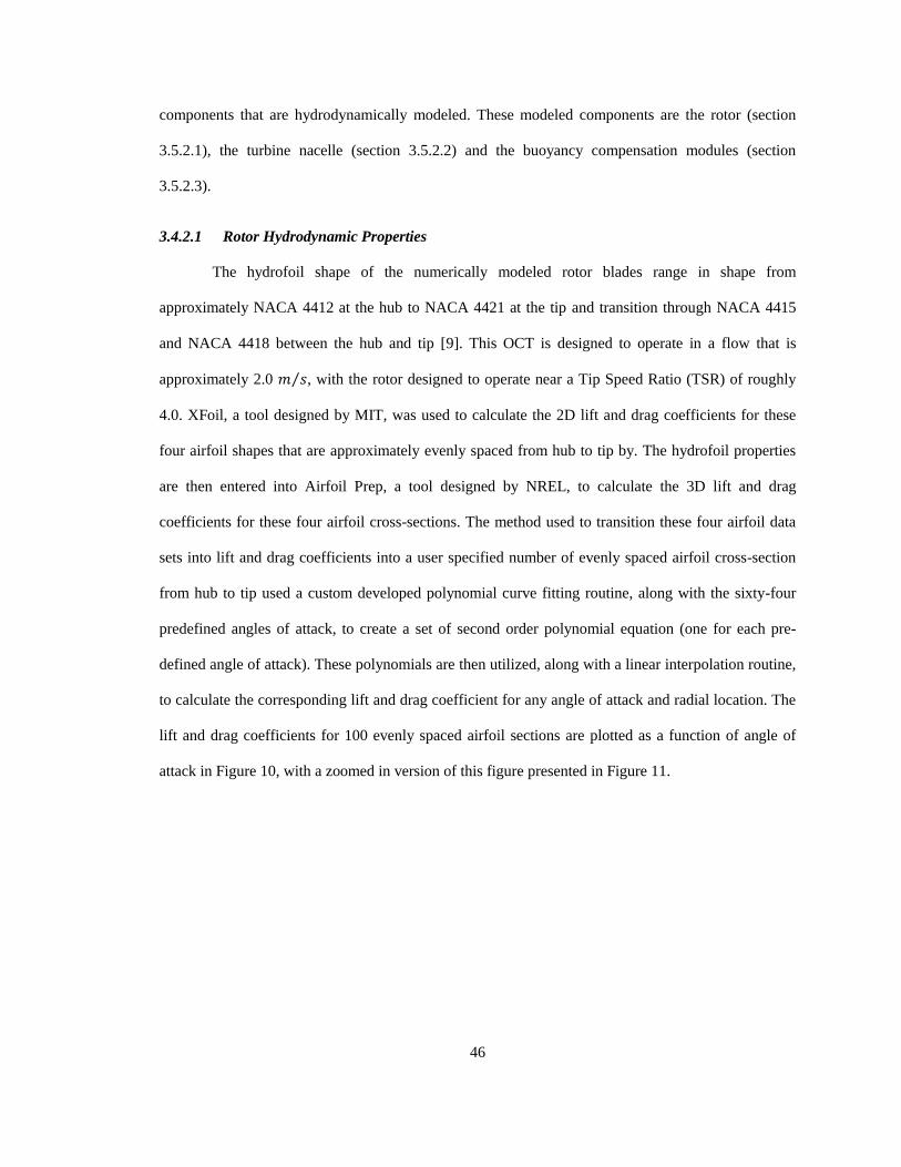
blade elements with respect to the rotor plane area. ................................................................ 10 Figure 5: Local loads on a blade ........................................................................................................... 11 Figure 6: Control Volume shaped as an annular element used with the BEM model ........................... 13 Figure 7: Image of OrcaFlex’s Coordinate systems .............................................................................. 20 Figure 8: Screen Shot of OrcaFlex’s Graphic User Interface. ............................................................... 21 Figure 9: Lumped buoy coordinate system. .......................................................................................... 30 Figure 10: 3D Lift and Drag Coefficient as angle a function of attack for all possible angles of
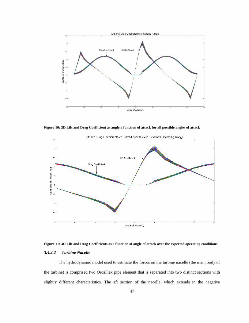
attack ....................................................................................................................................... 47 Figure 11: 3D Lift and Drag Coefficients as a function of angle of attack over the expected
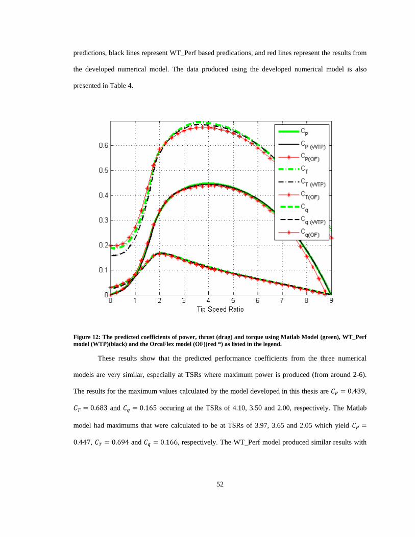
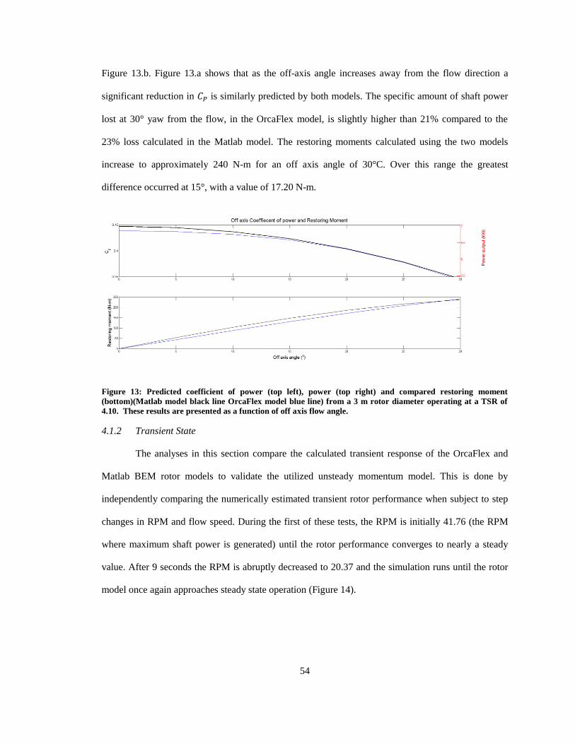
operating conditions ................................................................................................................ 47 Figure 12: The predicted coefficients of power, thrust (drag) and torque ............................................. 52 Figure 13: Predicted coefficient of power (top left), power (top right) and restoring moment
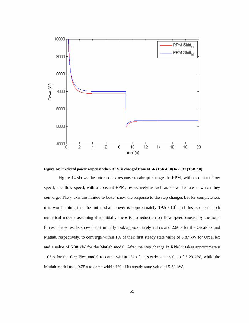
comparison from a 3 m rotor diameter operating at a TSR of 4.10. ........................................ 54 Figure 14: Predicted power response when RPM is changed from 41.76 (TSR 4.10) to 20.37 (TSR
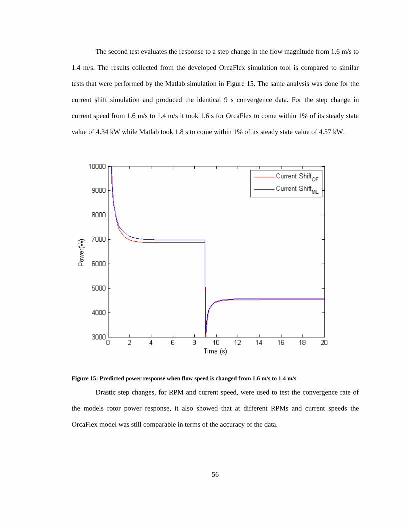
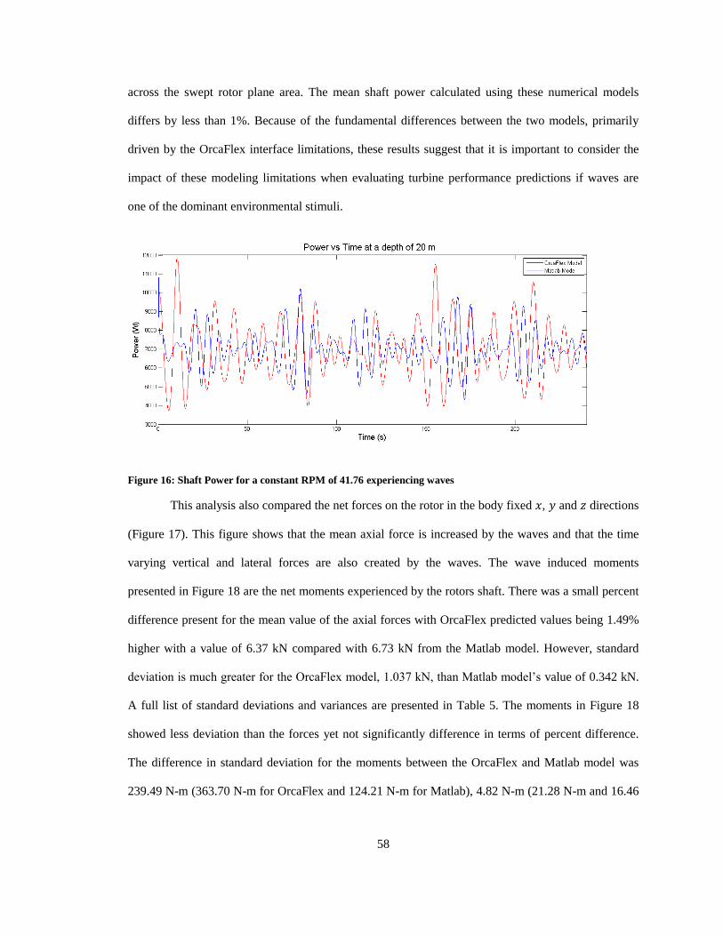
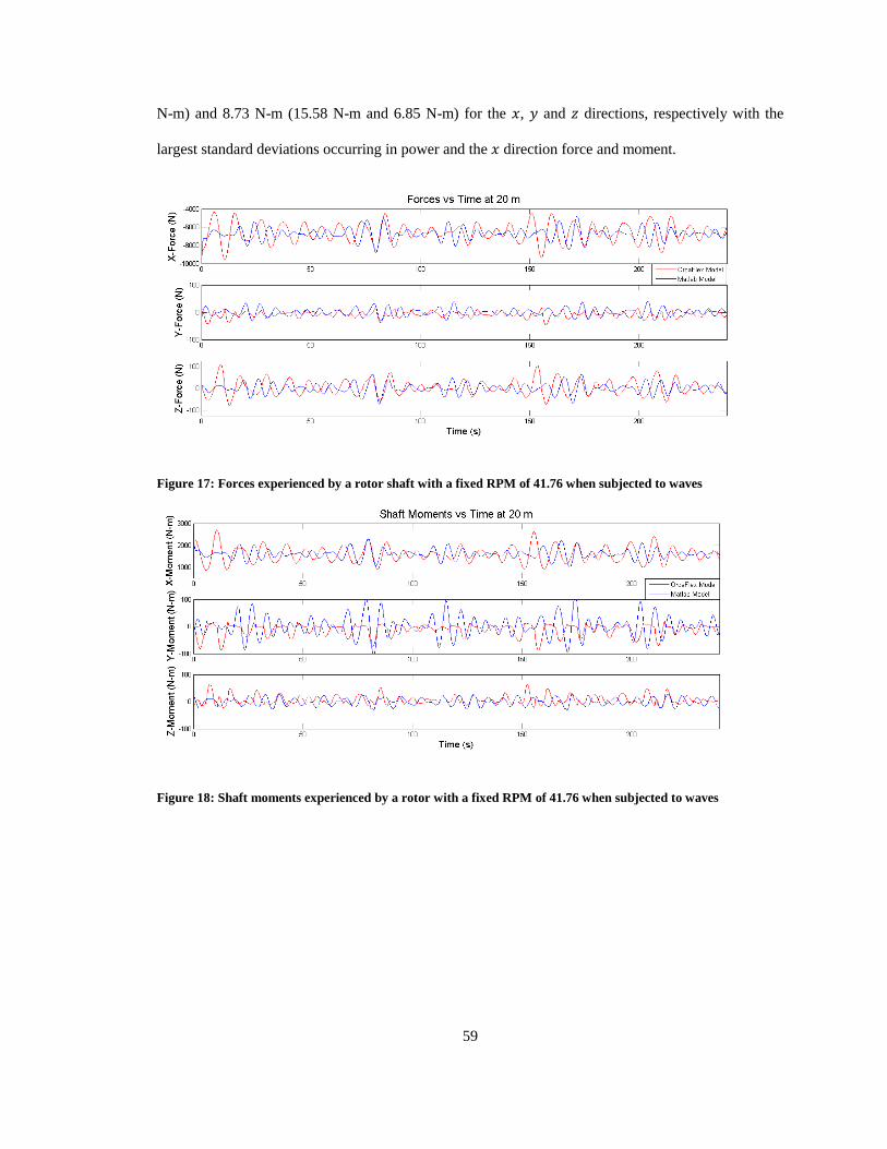
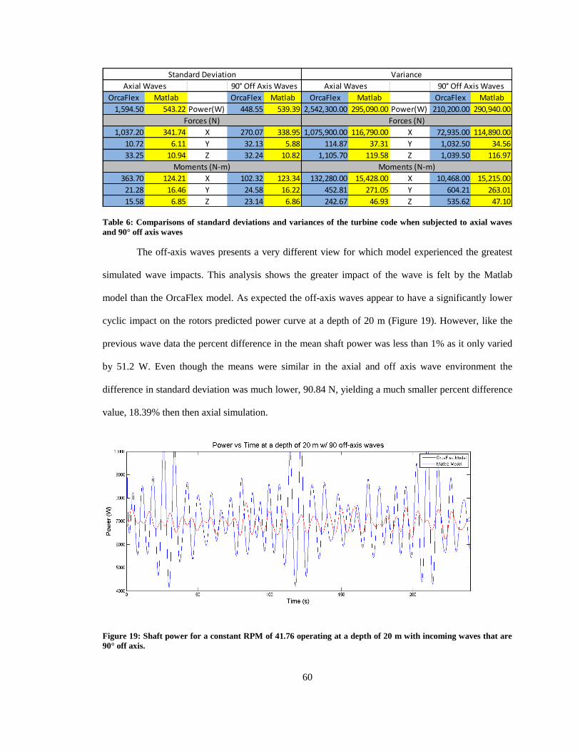
2.0) ........................................................................................................................................... 55 Figure 15: Predicted power response when flow speed is changed from 1.6 m/s to 1.4 m/s ................ 56 Figure 16: Shaft Power for a constant RPM of 41.76 experiencing waves ........................................... 58 Figure 17: Forces experienced by a rotor shaft with a fixed RPM of 41.76 when subjected to
waves ....................................................................................................................................... 59 Figure 18: Shaft moments experienced by a rotor with a fixed RPM of 41.76 when subjected to
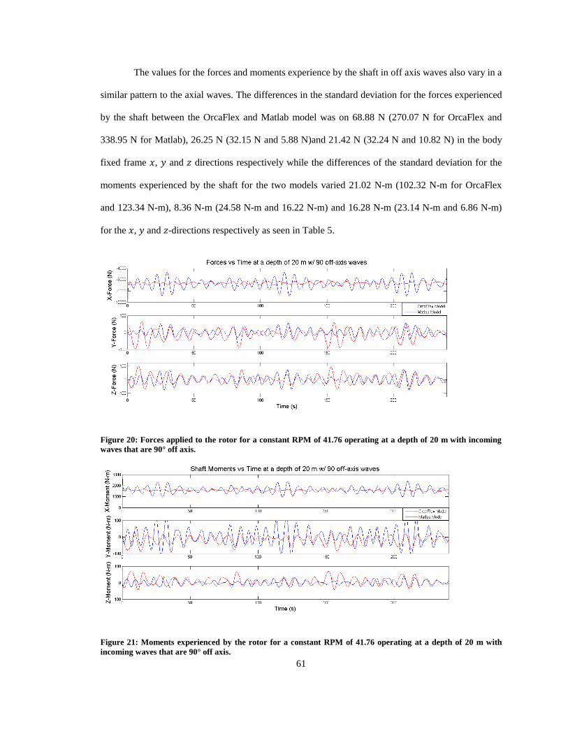
waves ....................................................................................................................................... 59 Figure 19: Shaft power for a constant RPM of 41.76 operating at a depth of 20 m with incoming
waves that are 90° off axis. ...................................................................................................... 60 Figure 20: Forces applied to the rotor for a constant RPM of 41.76 operating at a depth of 20 m
with incoming waves that are 90° off axis............................................................................... 61 Figure 21: Moments experienced by the rotor for a constant RPM of 41.76 operating at a depth of
20 m with incoming waves that are 90° off axis. .................................................................... 61 Figure 22: Mooring configuration utilized to simulate OCT performance in a uniform steady
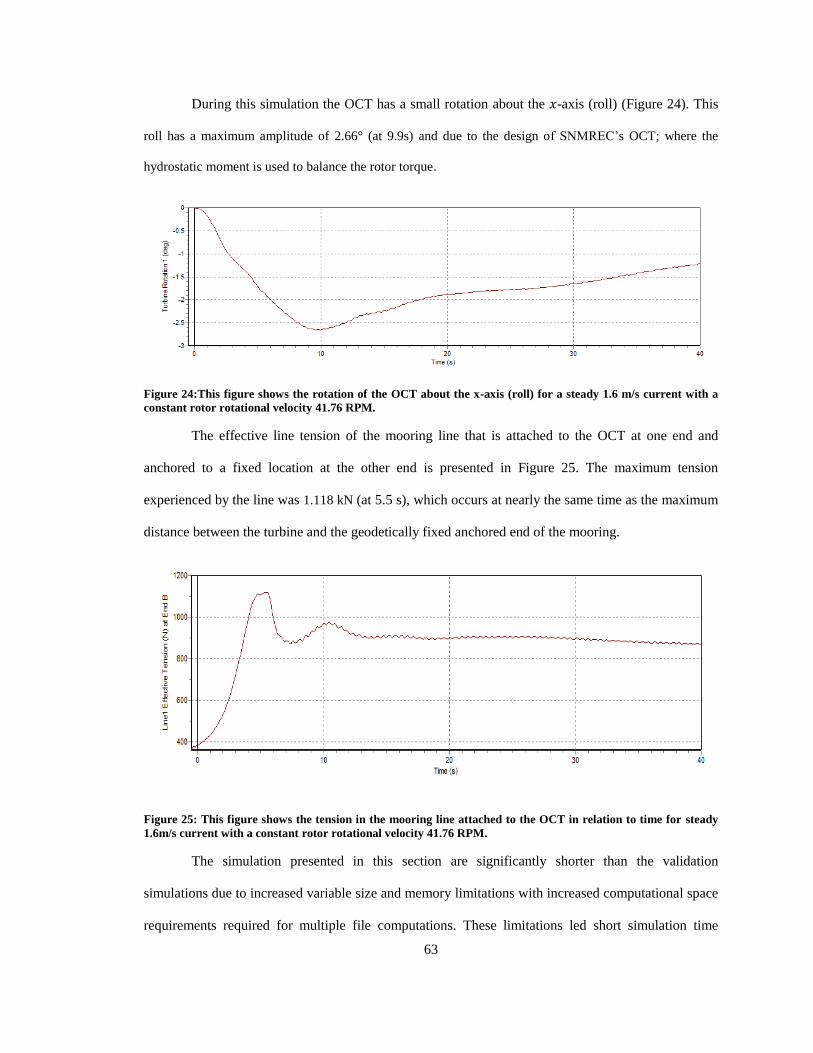
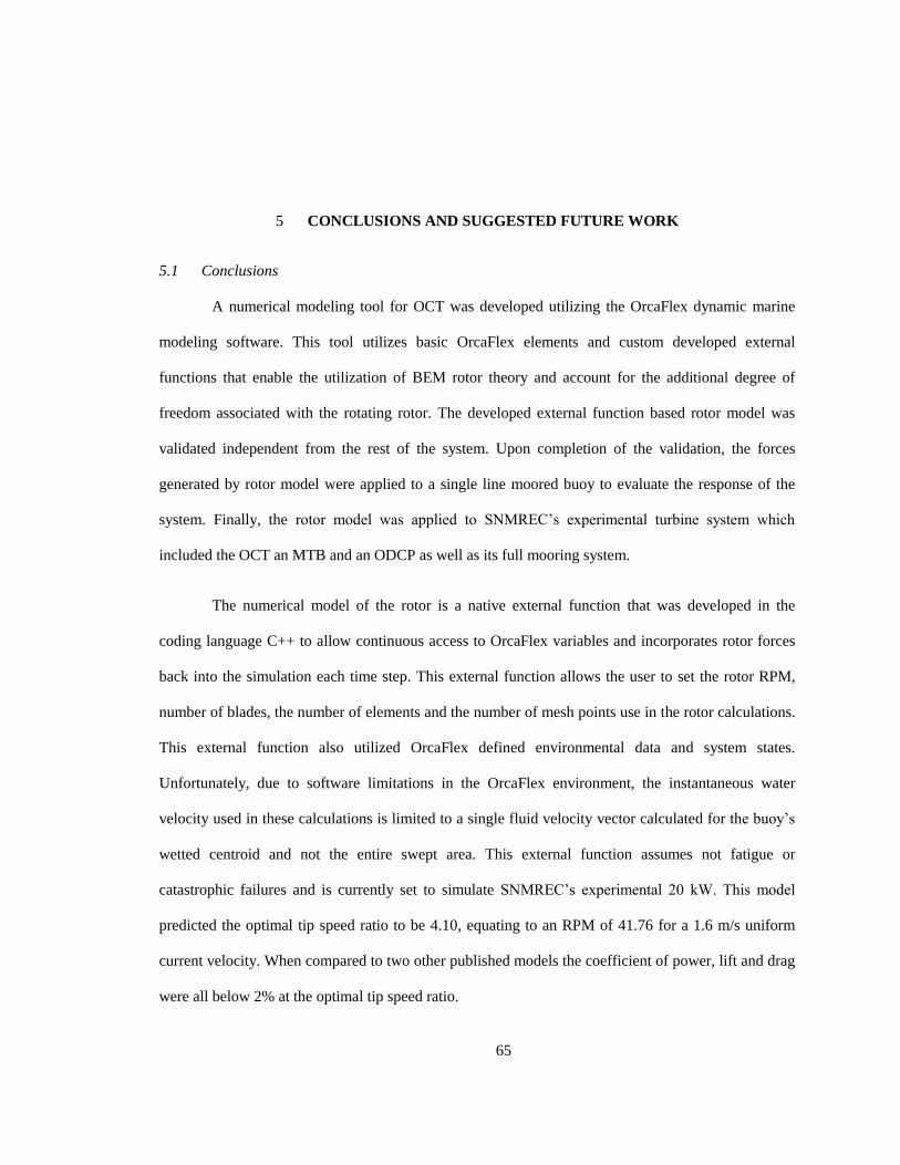
current ...................................................................................................................................... 62 Figure 23: This figure shows the power versus time for the rotor for a steady 1.6 m/s current ............ 62 Figure 24:This figure shows the rotation of the OCT about the x-axis (roll) for a steady 1.6 m/s
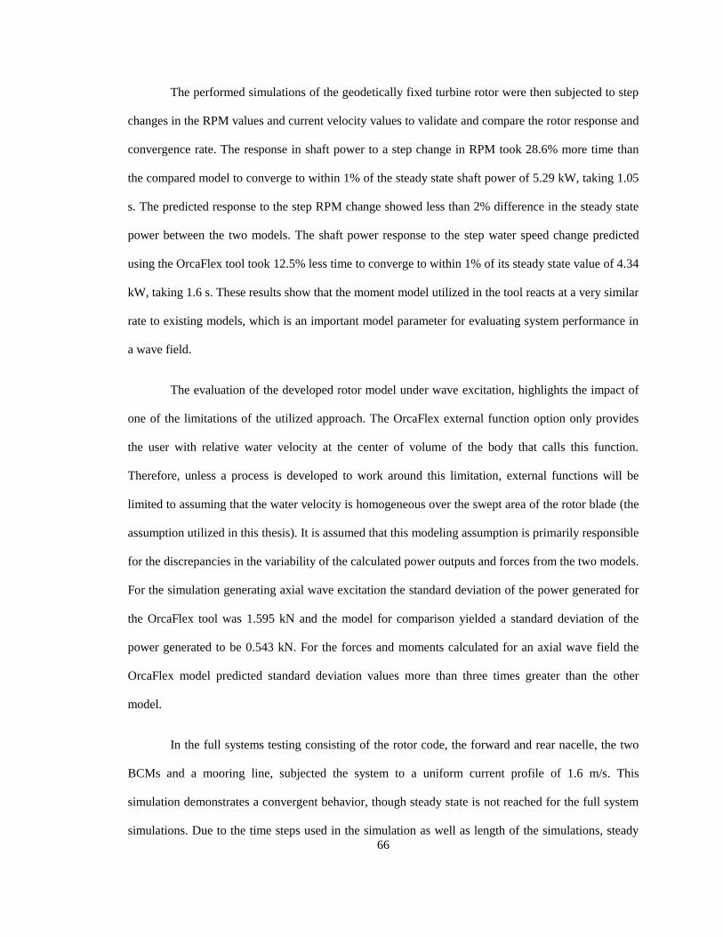
current with a constant rotor rotational velocity 41.76 RPM................................................... 63 Figure 25: This figure shows the tension in the mooring line attached to the OCT in relation to
time for steady 1.6m/s current with a constant rotor rotational velocity 41.76 RPM. ............. 63
ix
LIST OF TABLES
Table 1: Eight top HYCOM estimated regions in the world capable of providing hydrokinetic
current energy on a large scale, along with their respective areas above three power
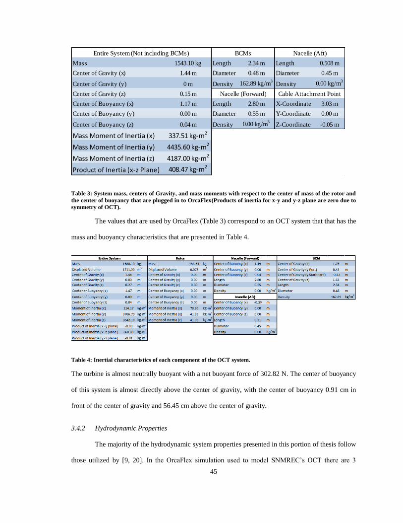
intensity thresholds. ................................................................................................................... 2 Table 2: Some of SNMREC’s Ocean Current Turbines predicted specifications ................................... 7 Table 3: System mass, centers of Gravity, and mass moments with respect to the center of mass of
the rotor and the center of buoyancy that are plugged in to OrcaFlex(Products of inertia
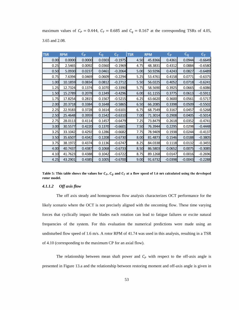
for x-y and y-z plane are zero due to symmetry of OCT). ....................................................... 45 Table 4: Inertial characteristics of each component of the OCT system. .............................................. 45 Table 5: This table shows the values for , and at a flow speed of 1.6 m⁄s calculated
using the developed rotor model. ............................................................................................ 53 Table 6: Comparisons of standard deviations and variances of the turbine code when subjected to
axial waves and 90° off axis waves ......................................................................................... 60
1
1 INTRODUCTION AND OBJECTIVES
1.1 Motivation
In order to cope with the increasing demand of energy, people have begun looking to the sea
where they found a large, clean renewable source that avoids many of the environmental issues which
arise from our current major methods of producing electricity. The oceans embody a vast amount of
heat and mechanical energy, which continually moves an enormous volume of water [1]. Within the
vast ocean there are a multitude of sources from which electricity can be extracted; such as ocean
thermal gradients, offshore wind and ocean kinetic energy in the forms of waves and currents. It has
been estimated that the ocean stores enough energy in the form of heat, currents, waves, and tides to
meet total worldwide demand for power many times over [2]. Hydrokinetic and wind power seem to
be the optimal choices in renewable energy sources of today due in large part to the number of sites
that they can be utilized [3], though another potential contender for marine renewable energy
production in the tropics and sub-tropics is ocean thermal energy.
Focusing on the hydrokinetic energy available within the ocean, there are essentially two
means of generating electricity from marine and tidal currents: a) building a tidal barrage across high
tide areas, some including estuaries or bays and b) extracting energy from free-flowing water in the
open ocean [4]. The first mentioned extraction methodology harnesses the potential energy but
presents several issues due their high construction costs and extreme environmental impact [5].Due to
the issues related to this method, alternative means were developed to harness the kinetic energy in
marine currents by placing Marine Hydro-Kinetic Turbines (MHKTs) to absorb the energy in the
water’s velocity without significantly impeding the flow [6].These devices can harness hydrokinetic
energy from river current, tidal current and open ocean currents, the latter of which is the focus of this
thesis.
2
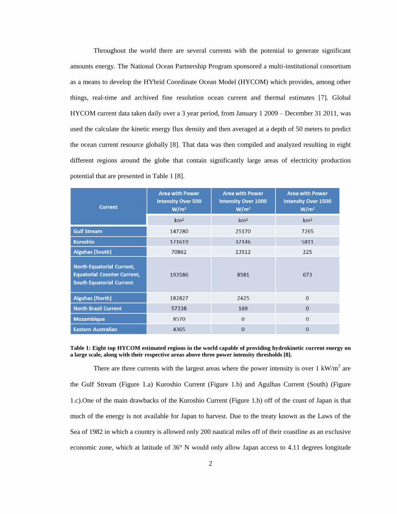
Throughout the world there are several currents with the potential to generate significant
amounts energy. The National Ocean Partnership Program sponsored a multi-institutional consortium
as a means to develop the HYbrid Coordinate Ocean Model (HYCOM) which provides, among other
things, real-time and archived fine resolution ocean current and thermal estimates [7]. Global
HYCOM current data taken daily over a 3 year period, from January 1 2009 – December 31 2011, was
used the calculate the kinetic energy flux density and then averaged at a depth of 50 meters to predict
the ocean current resource globally [8]. That data was then compiled and analyzed resulting in eight
different regions around the globe that contain significantly large areas of electricity production
potential that are presented in Table 1 [8].
Table 1: Eight top HYCOM estimated regions in the world capable of providing hydrokinetic current energy on
a large scale, along with their respective areas above three power intensity thresholds [8].
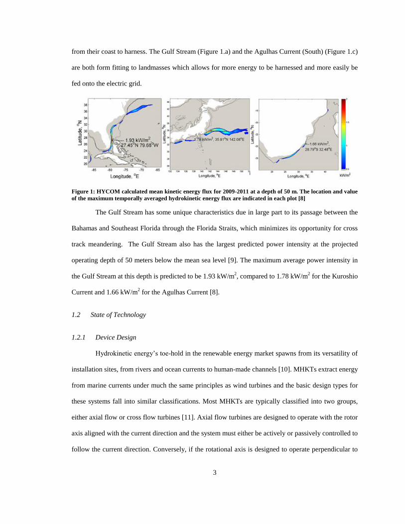
There are three currents with the largest areas where the power intensity is over 1 kW/m2 are
the Gulf Stream (Figure 1.a) Kuroshio Current (Figure 1.b) and Agulhas Current (South) (Figure
1.c).One of the main drawbacks of the Kuroshio Current (Figure 1.b) off of the coast of Japan is that
much of the energy is not available for Japan to harvest. Due to the treaty known as the Laws of the
Sea of 1982 in which a country is allowed only 200 nautical miles off of their coastline as an exclusive
economic zone, which at latitude of 36° N would only allow Japan access to 4.11 degrees longitude
3
from their coast to harness. The Gulf Stream (Figure 1.a) and the Agulhas Current (South) (Figure 1.c)
are both form fitting to landmasses which allows for more energy to be harnessed and more easily be
fed onto the electric grid.
Figure 1: HYCOM calculated mean kinetic energy flux for 2009-2011 at a depth of 50 m. The location and value
of the maximum temporally averaged hydrokinetic energy flux are indicated in each plot [8]
The Gulf Stream has some unique characteristics due in large part to its passage between the
Bahamas and Southeast Florida through the Florida Straits, which minimizes its opportunity for cross
track meandering. The Gulf Stream also has the largest predicted power intensity at the projected
operating depth of 50 meters below the mean sea level [9]. The maximum average power intensity in
the Gulf Stream at this depth is predicted to be 1.93 kW/m2, compared to 1.78 kW/m
2 for the Kuroshio
Current and 1.66 kW/m2 for the Agulhas Current [8].
1.2 State of Technology
1.2.1 Device Design
Hydrokinetic energy’s toe-hold in the renewable energy market spawns from its versatility of
installation sites, from rivers and ocean currents to human-made channels [10]. MHKTs extract energy
from marine currents under much the same principles as wind turbines and the basic design types for
these systems fall into similar classifications. Most MHKTs are typically classified into two groups,
either axial flow or cross flow turbines [11]. Axial flow turbines are designed to operate with the rotor
axis aligned with the current direction and the system must either be actively or passively controlled to
follow the current direction. Conversely, if the rotational axis is designed to operate perpendicular to
4
the current the flow direction is not important and this design type is referred to as a cross flow turbine
[12]. Axial flow turbines currently have achieved a dominant position in the turbine market, with most
open ocean designs utilizing this rotor type [2, 13, 14, 15]. Most MHKT systems are designed to be
either bottom mounted or moored, but our focus will be on the moored designs since this is the only
feasible method for most open ocean locations.
As with most emerging technologies MHKTs still have several obstacles to overcome before
becoming a fully viable asset in harnessing the energy of the ocean currents. One of the largest hurdles
is designing a system that anchors the turbine to the ground while allowing it to operate near the
surface and align itself with the current. Another hurdle lies in the deployment, operation, and
maintenance and retrieval stage of a MHKT system in the open ocean.
1.2.2 Simulation Developments
Due to some of the hurdles mentioned above the MHKT industry’s is making slow but steady
progress towards deploying systems in the open ocean. Without means to easily test and simulate
designs it is difficult to predict what designs stand the best chance at working, avoiding failures, and
creating electricity that is economically sustainable. An important step towards getting MHKTs
operating in the open ocean is to create a tool that developers can use to simulate the performance of
their coupled turbine and mooring designs.
When modeling large complex systems such as a moored MHKT designed to operate in the
open ocean, it is important to study both the forces on the rotor and the coupled affects that the rotor
and environment have on the moored system as a whole. To model these coupled interactions, rotor
and turbine systems can be modeled and simulated with time domain approaches that account for
system motion when calculating the fluid loadings on the structure. Using this approach, researchers
have gained an initial understanding of the behavior of OCT systems when operating in an offshore
environment [9, 16]. This approach allows all the parts of a complete system to work together without
limiting the ability of each component to be analyzed separately. In order to accurately simulate the
relationship between a rotor and the flow of a fluid body through the swept rotor plane area in a
5
dynamic environment it is important to know both the undisturbed flow at the current time step and
the flow reduction caused by the rotor on the flow from the wake of the previous time steps [17]. This
adds complexity to creating numeric models since numeric modeling programs such as OrcaFlex
assume that the flow is undisturbed by the structure for all of its standard calculations.
Recently, two numerical simulation models have be developed, the first of which utilizes a
BEM rotor model and is implemented in MATLAB/Simulink[18] and the second of which utilizes a
Blade Element (BE) rotor model and is implemented in OrcaFlex [19,20]. The MATLAB model
utilizes several different corrections/modifications to the traditional BEM model that allow it to
account for shear currents and waves. One drawback to this numeric model is that it utilizes a
somewhat basic cable model that limits its usefulness for analyzing commercial OCT systems, which
utilize complex mooring system. A second drawback to this numeric model is that it does not have a
user interface and requires both basic programming skills and experience with numeric simulations to
create meaningful results. The OrcaFlex model, by only incorporating the basic BE rotor model, has
significant inaccuracies in rotor performance calculations and was designed more to analyze the
behavior of the mooring system than the turbine itself. By combining the accurate rotor model
implemented in [18] with the mooring simulation model [19, 20] into a single tool with the best
features of both models, OCT developers will be better equipped to evaluate prototyped systems.
1.3 SNMREC’s Experimental OCT
The Southeast National Marine Renewable Energy Center (SNMREC) has developed an
experiment 3.08 m rotor diameter Ocean Current Turbine (OCT) that is designed to work in open
ocean conditions and generate approximately 20 kW of power in 2.3m/s while operating at a tip speed
around 5.0 [9]. The preliminary design can be seen in Figure 2.
6
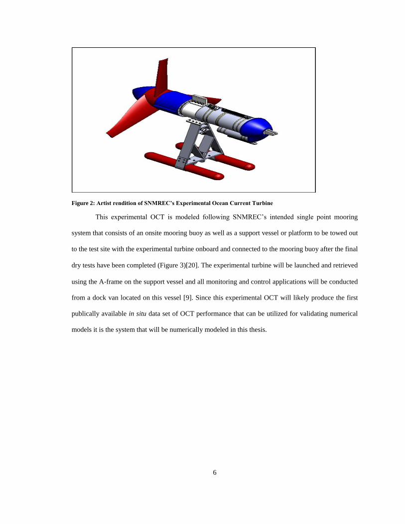
Figure 2: Artist rendition of SNMREC’s Experimental Ocean Current Turbine
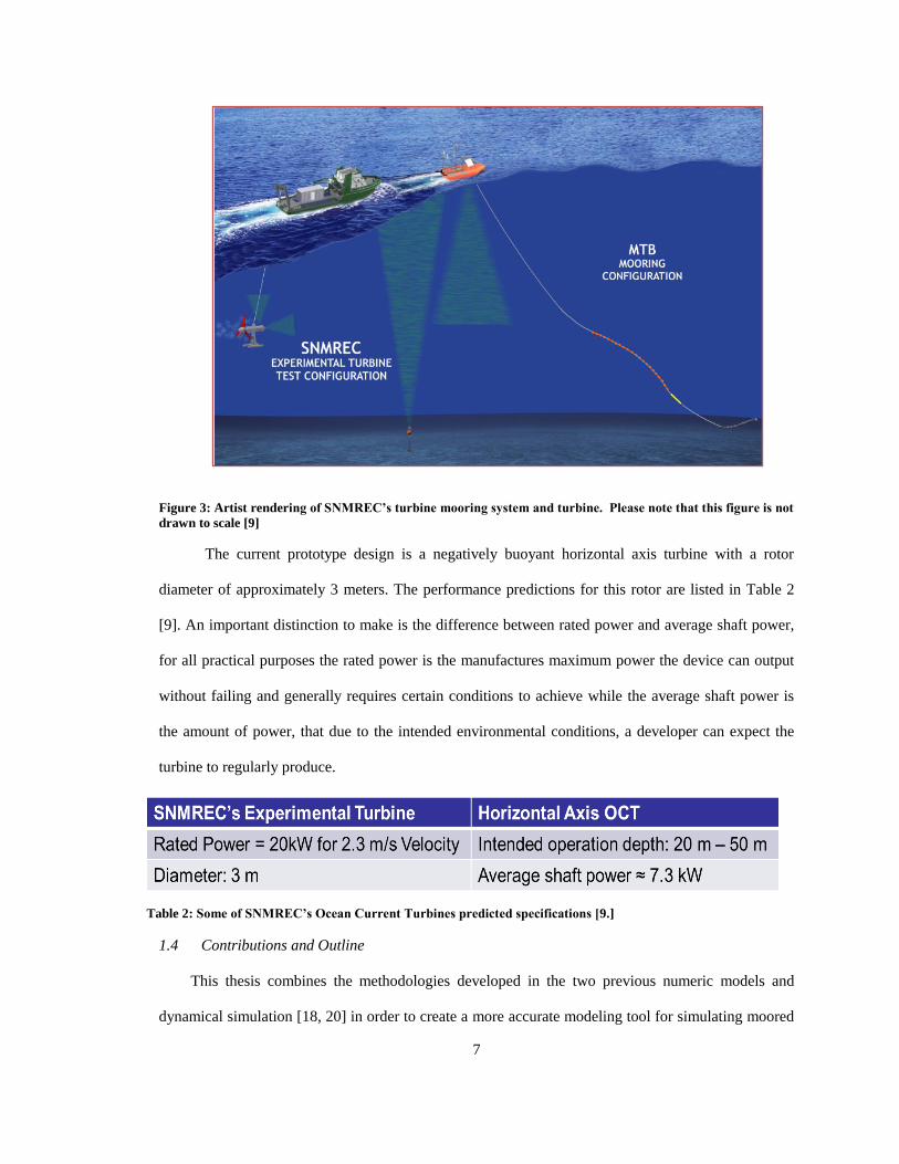
This experimental OCT is modeled following SNMREC’s intended single point mooring
system that consists of an onsite mooring buoy as well as a support vessel or platform to be towed out
to the test site with the experimental turbine onboard and connected to the mooring buoy after the final
dry tests have been completed (Figure 3)[20]. The experimental turbine will be launched and retrieved
using the A-frame on the support vessel and all monitoring and control applications will be conducted
from a dock van located on this vessel [9]. Since this experimental OCT will likely produce the first
publically available in situ data set of OCT performance that can be utilized for validating numerical
models it is the system that will be numerically modeled in this thesis.
7
Figure 3: Artist rendering of SNMREC’s turbine mooring system and turbine. Please note that this figure is not
drawn to scale [9]
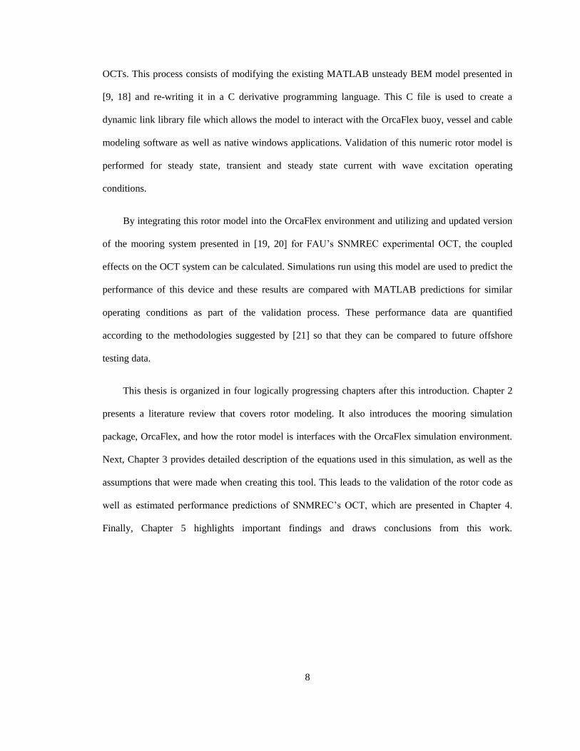
The current prototype design is a negatively buoyant horizontal axis turbine with a rotor
diameter of approximately 3 meters. The performance predictions for this rotor are listed in Table 2
[9]. An important distinction to make is the difference between rated power and average shaft power,
for all practical purposes the rated power is the manufactures maximum power the device can output
without failing and generally requires certain conditions to achieve while the average shaft power is
the amount of power, that due to the intended environmental conditions, a developer can expect the
turbine to regularly produce.
1.4 Contributions and Outline
This thesis combines the methodologies developed in the two previous numeric models and
dynamical simulation [18, 20] in order to create a more accurate modeling tool for simulating moored
Table 2: Some of SNMREC’s Ocean Current Turbines predicted specifications [9.]
8
OCTs. This process consists of modifying the existing MATLAB unsteady BEM model presented in
[9, 18] and re-writing it in a C derivative programming language. This C file is used to create a
dynamic link library file which allows the model to interact with the OrcaFlex buoy, vessel and cable
modeling software as well as native windows applications. Validation of this numeric rotor model is
performed for steady state, transient and steady state current with wave excitation operating
conditions.
By integrating this rotor model into the OrcaFlex environment and utilizing and updated version
of the mooring system presented in [19, 20] for FAU’s SNMREC experimental OCT, the coupled
effects on the OCT system can be calculated. Simulations run using this model are used to predict the
performance of this device and these results are compared with MATLAB predictions for similar
operating conditions as part of the validation process. These performance data are quantified
according to the methodologies suggested by [21] so that they can be compared to future offshore
testing data.
This thesis is organized in four logically progressing chapters after this introduction. Chapter 2
presents a literature review that covers rotor modeling. It also introduces the mooring simulation
package, OrcaFlex, and how the rotor model is interfaces with the OrcaFlex simulation environment.
Next, Chapter 3 provides detailed description of the equations used in this simulation, as well as the
assumptions that were made when creating this tool. This leads to the validation of the rotor code as
well as estimated performance predictions of SNMREC’s OCT, which are presented in Chapter 4.
Finally, Chapter 5 highlights important findings and draws conclusions from this work.
9
2 LITERATURE REVIEW
This chapter covers two fundamental areas that this thesis builds upon. First, several rotor
modeling approaches are discussed, with a focus on the Blade Element Momentum rotor modeling
technique utilized in this thesis. This discussion introduces the fundamental Blade Element Model and
Momentum Model and then discusses modifications that that have been developed so that these
fundamental theories can be used in an operating environment where the fluid and rotor velocities
vary both in time and space. Following this discussion some of the relevant characteristics of the
numeric modeling platform that is utilized in this thesis, OrcaFlex, are discussed. This includes a
general overview of how this modeling platform operates followed by more discussion of OrcaFlex’s
“external function”, a function that allows the user to incorporate custom numerical models into its
operating environment.
2.1 Rotor Modeling
When numerically predicting rotor performance there are many techniques that can be used
including but not limited to: Generalized Dynamic Wake Model (GDW) [22] to Strip Theory or Blade
Element Momentum (BEM) model [23] and Vortex Lattice Method [24,25] just to name a few. The
method that is utilized in this application will be a modified version of the Blade Element Momentum
method and will build upon the work of [18, 9]. The BEM model, in its most basic form, is designed
to model rotor behavior in a steady state [17, 26]. With a few adaptations that will be explained in
Subsections 2.1.2 and 2.1.3 this approach can be modified to allow the BEM model to work for
unsteady states and also increase its accuracy [17].
2.1.1 Basic Blade Element Momentum Model
The BEM model is comprised of two different yet related theories; the blade element theory and
the momentum theory [23]. Betz concluded that the BEM model works by breaking a lifting surface
10
into discrete elements and then calculating the effect that the rotating blade has on the flow at each
element. By monitoring the flow past each elemental lifting surface the forces on the rotor and power
generated by our turbine can be calculated. Glauert applied the angular momentum method, discussed
in Section 2.1.1.2, to concentric annuli that correspond with the existing Blade Element Model [27],
discussed in Section 2.1.1.1. Glauert also added an expression for the angular momentum balance, in
which changes in the angular momentum (from the free stream value of zero) are equated to the torque
exerted by the rotor on the fluid. This involves the introduction of a tangential or angular induction
velocity to manage the relationship between velocities at different locations [28].
2.1.1.1 Blade Element Model
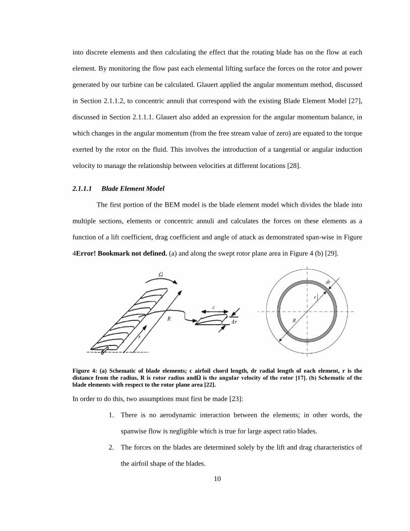
The first portion of the BEM model is the blade element model which divides the blade into
multiple sections, elements or concentric annuli and calculates the forces on these elements as a
function of a lift coefficient, drag coefficient and angle of attack as demonstrated span-wise in Figure
4Error! Bookmark not defined. (a) and along the swept rotor plane area in Figure 4 (b) [29].
Figure 4: (a) Schematic of blade elements; c airfoil chord length, dr radial length of each element, r is the
distance from the radius, R is rotor radius andΩ is the angular velocity of the rotor [17]. (b) Schematic of the
blade elements with respect to the rotor plane area [22].
In order to do this, two assumptions must first be made [23]:
1. There is no aerodynamic interaction between the elements; in other words, the
spanwise flow is negligible which is true for large aspect ratio blades.
2. The forces on the blades are determined solely by the lift and drag characteristics of
the airfoil shape of the blades.
11
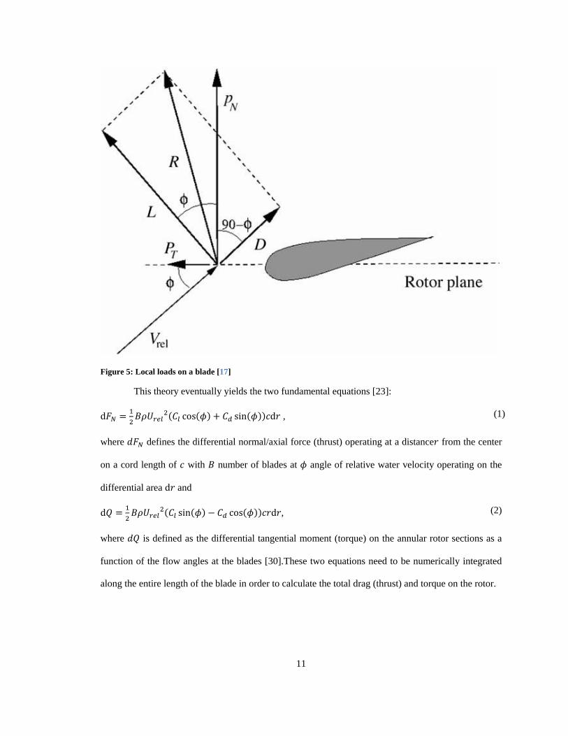
Figure 5: Local loads on a blade [17]
This theory eventually yields the two fundamental equations [23]:
( ( ) ( )) , (1)
where defines the differential normal/axial force (thrust) operating at a distance from the center
on a cord length of with number of blades at angle of relative water velocity operating on the
differential area and
( ( ) ( )) , (2)
where is defined as the differential tangential moment (torque) on the annular rotor sections as a
function of the flow angles at the blades [30].These two equations need to be numerically integrated
along the entire length of the blade in order to calculate the total drag (thrust) and torque on the rotor.
12
2.1.1.2 Momentum Model
Momentum theory takes an annular control volume approach that utilized the forces at the
blade to calculate the reduced incoming flow velocity based on the conservation of linear and angular
momentum [23]. This is achieved with the understanding that forces on the rotor blade and the flow
conditions at the rotor blade are related by the balance of momentum, since force is simply the rate of
change of momentum. By using the annular control volume the angular and axial induction factors can
be assumed to be a function of the radius [17]. In the momentum model some of the axial flow is
deflected away from the turbine which results in the flow past the rotor to have a velocity less than the
free stream velocity, the axial induction factor is the ratio of this velocity loss in the far-field.
By applying the conservation of linear momentum to the annular control volume of radius
and thickness the differential contribution of thrust can be expressed as suggested by [23],
( ) , (3)
where is the differential thrust, is the density of the fluid body, is the axial induction factor and
is the radial length. Similarly, the conservation of angular momentum equation allows the torque to
be calculated as suggested by [23],
( ) , (4)
where is the tangential induction factor and is the rotational velocity. Thus, thrust and
torque on each annular section of the rotor can be defined as a function of the axial and angular
induction factors or in other words, the flow conditions [23]. The tangential induction factor, also
known as the wake rotation, is the ratio of the rotational velocity that has been lost by passing through
the rotor and the free stream rotational velocity. Unfortunately the simple momentum theory alone
provides only an initial idea regarding the how well a propeller or turbine may perform, but does not
provide enough sufficient enough information to allow for detailed design [29].
2.1.2 Complete Blade Element Momentum Model
This section ties the previous two sub-sections, the Momentum model and the Blade Element
model, together to introduce the Blade Element Momentum model. These two models are then joined
13
together by incorporating the geometry of the into the annular control volume. The characteristics of
the blade such as local cord length, angle of attach and lift and drag coefficients are included in the
equations for force. The momentum It also introduces adjustments that have been made to the original
model to increase its accuracy. These include Prandtl’s tip loss factor and Glauert’s Correction for
High Values of .
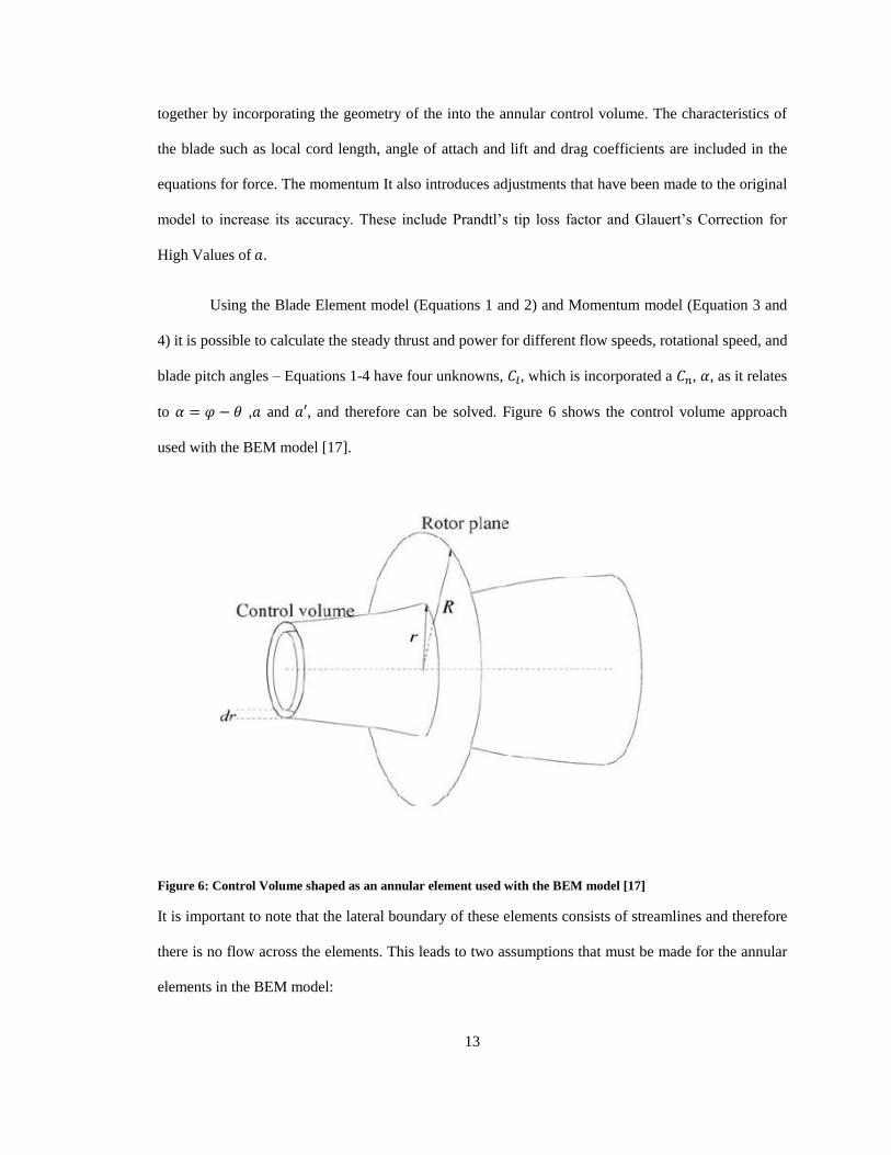
Using the Blade Element model (Equations 1 and 2) and Momentum model (Equation 3 and
4) it is possible to calculate the steady thrust and power for different flow speeds, rotational speed, and
blade pitch angles – Equations 1-4 have four unknowns, , which is incorporated a , , as it relates
to , and , and therefore can be solved. Figure 6 shows the control volume approach
used with the BEM model [17].
Figure 6: Control Volume shaped as an annular element used with the BEM model [17]
It is important to note that the lateral boundary of these elements consists of streamlines and therefore
there is no flow across the elements. This leads to two assumptions that must be made for the annular
elements in the BEM model:
14
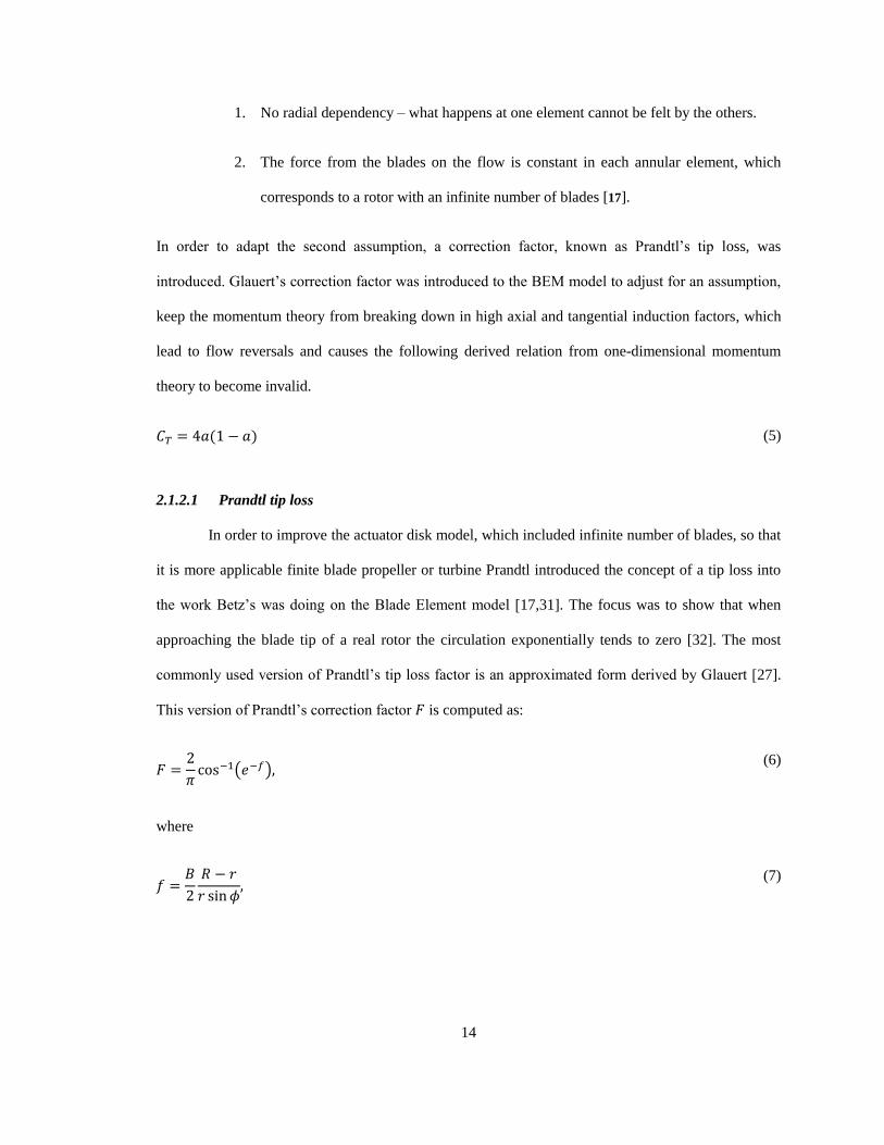
1. No radial dependency – what happens at one element cannot be felt by the others.
2. The force from the blades on the flow is constant in each annular element, which
corresponds to a rotor with an infinite number of blades [17].
In order to adapt the second assumption, a correction factor, known as Prandtl’s tip loss, was
introduced. Glauert’s correction factor was introduced to the BEM model to adjust for an assumption,
keep the momentum theory from breaking down in high axial and tangential induction factors, which
lead to flow reversals and causes the following derived relation from one-dimensional momentum
theory to become invalid.
( ) (5)
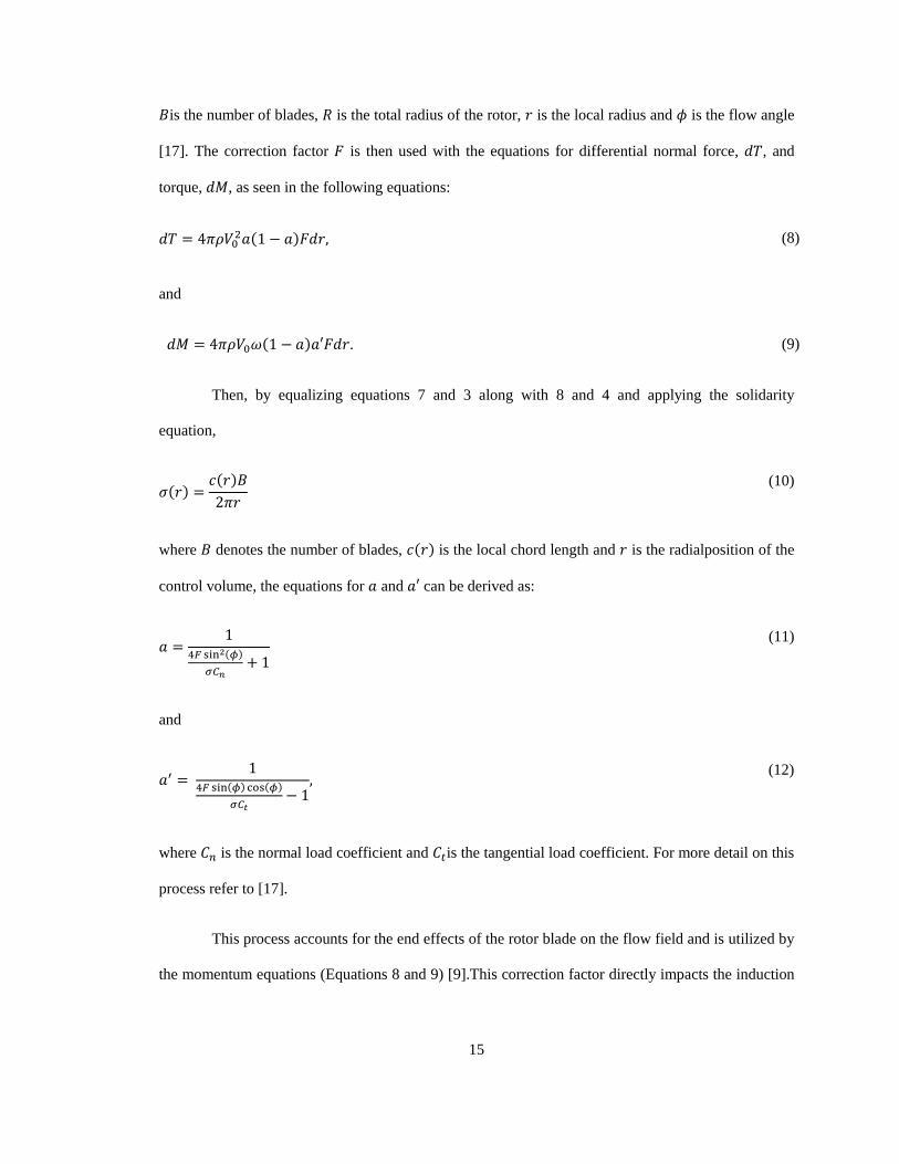
2.1.2.1 Prandtl tip loss
In order to improve the actuator disk model, which included infinite number of blades, so that
it is more applicable finite blade propeller or turbine Prandtl introduced the concept of a tip loss into
the work Betz’s was doing on the Blade Element model [17,31]. The focus was to show that when
approaching the blade tip of a real rotor the circulation exponentially tends to zero [32]. The most
commonly used version of Prandtl’s tip loss factor is an approximated form derived by Glauert [27].
This version of Prandtl’s correction factor is computed as:
( )
(6)
where
(7)
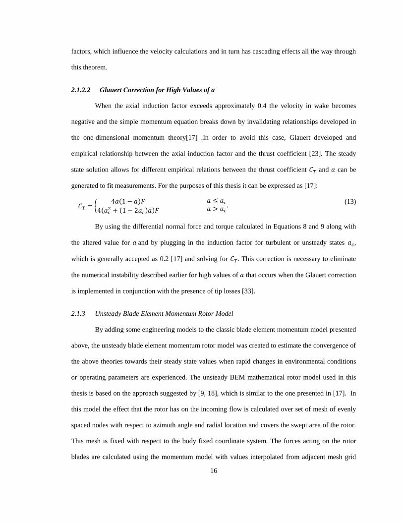
15
is the number of blades, is the total radius of the rotor, is the local radius and is the flow angle
[17]. The correction factor is then used with the equations for differential normal force, , and
torque, , as seen in the following equations:
( ) (8)
and
( ) . (9)
Then, by equalizing equations 7 and 3 along with 8 and 4 and applying the solidarity
equation,
( ) ( )
(10)
where denotes the number of blades, ( ) is the local chord length and is the radialposition of the
control volume, the equations for and can be derived as:
( )
(11)
and
( ) ( )
(12)
where is the normal load coefficient and is the tangential load coefficient. For more detail on this
process refer to [17].
This process accounts for the end effects of the rotor blade on the flow field and is utilized by
the momentum equations (Equations 8 and 9) [9].This correction factor directly impacts the induction
16
factors, which influence the velocity calculations and in turn has cascading effects all the way through
this theorem.
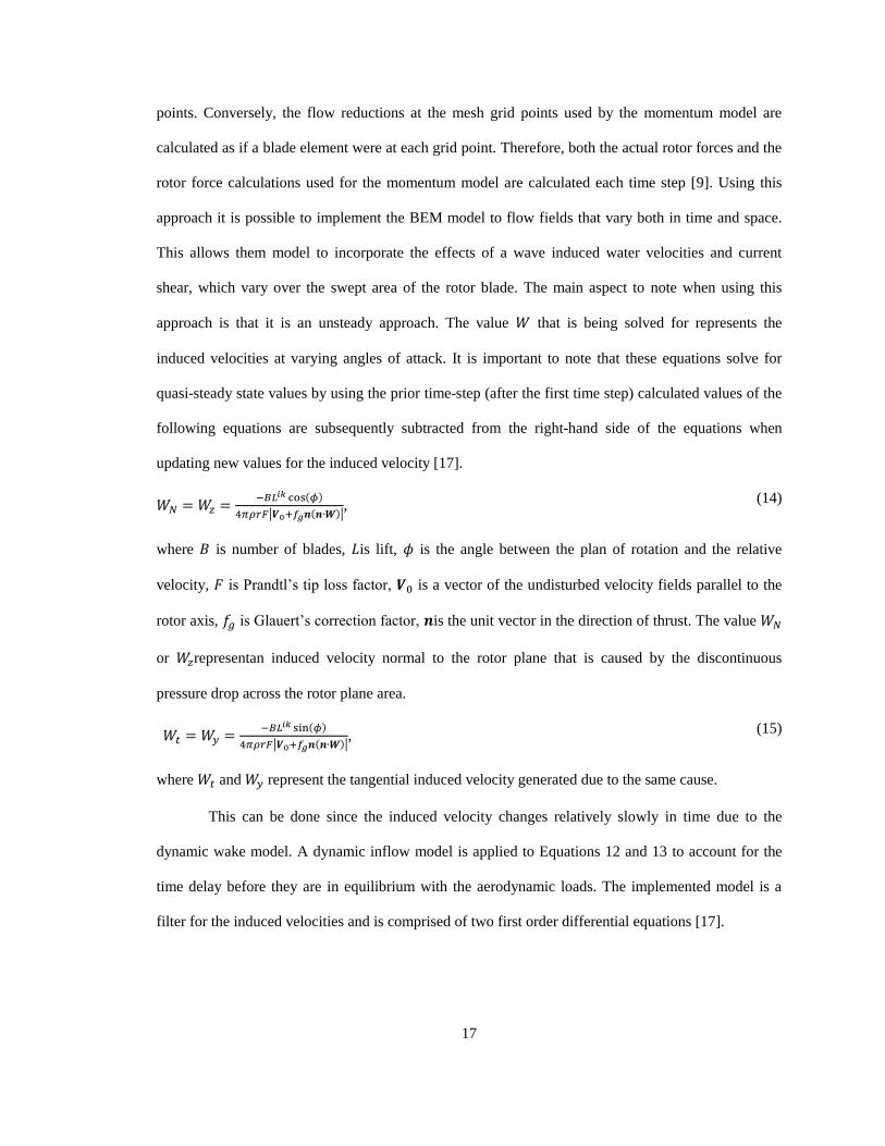
2.1.2.2 Glauert Correction for High Values of a
When the axial induction factor exceeds approximately 0.4 the velocity in wake becomes
negative and the simple momentum equation breaks down by invalidating relationships developed in
the one-dimensional momentum theory[17] .In order to avoid this case, Glauert developed and
empirical relationship between the axial induction factor and the thrust coefficient [23]. The steady
state solution allows for different empirical relations between the thrust coefficient and can be
generated to fit measurements. For the purposes of this thesis it can be expressed as [17]:
( )
( ( ) )
(13)
By using the differential normal force and torque calculated in Equations 8 and 9 along with
the altered value for and by plugging in the induction factor for turbulent or unsteady states ,
which is generally accepted as 0.2 [17] and solving for . This correction is necessary to eliminate
the numerical instability described earlier for high values of that occurs when the Glauert correction
is implemented in conjunction with the presence of tip losses [33].
2.1.3 Unsteady Blade Element Momentum Rotor Model
By adding some engineering models to the classic blade element momentum model presented
above, the unsteady blade element momentum rotor model was created to estimate the convergence of
the above theories towards their steady state values when rapid changes in environmental conditions
or operating parameters are experienced. The unsteady BEM mathematical rotor model used in this
thesis is based on the approach suggested by [9, 18], which is similar to the one presented in [17]. In
this model the effect that the rotor has on the incoming flow is calculated over set of mesh of evenly
spaced nodes with respect to azimuth angle and radial location and covers the swept area of the rotor.
This mesh is fixed with respect to the body fixed coordinate system. The forces acting on the rotor
blades are calculated using the momentum model with values interpolated from adjacent mesh grid
17
points. Conversely, the flow reductions at the mesh grid points used by the momentum model are
calculated as if a blade element were at each grid point. Therefore, both the actual rotor forces and the
rotor force calculations used for the momentum model are calculated each time step [9]. Using this
approach it is possible to implement the BEM model to flow fields that vary both in time and space.
This allows them model to incorporate the effects of a wave induced water velocities and current
shear, which vary over the swept area of the rotor blade. The main aspect to note when using this
approach is that it is an unsteady approach. The value that is being solved for represents the
induced velocities at varying angles of attack. It is important to note that these equations solve for
quasi-steady state values by using the prior time-step (after the first time step) calculated values of the
following equations are subsequently subtracted from the right-hand side of the equations when
updating new values for the induced velocity [17].
( )
| ( )|,
(14)
where is number of blades, is lift, is the angle between the plan of rotation and the relative
velocity, is Prandtl’s tip loss factor, is a vector of the undisturbed velocity fields parallel to the
rotor axis, is Glauert’s correction factor, is the unit vector in the direction of thrust. The value
or representan induced velocity normal to the rotor plane that is caused by the discontinuous
pressure drop across the rotor plane area.
( )
| ( )|,
(15)
where and represent the tangential induced velocity generated due to the same cause.
This can be done since the induced velocity changes relatively slowly in time due to the
dynamic wake model. A dynamic inflow model is applied to Equations 12 and 13 to account for the
time delay before they are in equilibrium with the aerodynamic loads. The implemented model is a
filter for the induced velocities and is comprised of two first order differential equations [17].
18
(16)
where is the quasi-steady value found in Equations 12 and 13 and is an intermediate value.
(17)
The value of is then the final filtered value to be used as the induced velocities and for more detail
in the two times constants and see [17].
2.2 OrcaFlex
While the Ocean Current Turbine simulation presented by [9] accounts for waves and current
shear, it is somewhat limited by its numeric cable model, which significantly slows the simulation
down when more than 5 cable elements are utilized. To allow device developers to more easily
numerically model OCT systems that utilize complex mooring system, the rotor model utilized by [9]
is modified and then implemented into the OrcaFlex numeric modeling program as part of this thesis.
OrcaFlex is one of the leading software packages for the dynamic analysis of offshore marine systems,
specializing in mooring systems, buoys and vessels [34]. The OrcaFlex environment allows users to
easily set and adjust their simulated operating environment and model properties when evaluating
their systems. Unfortunately, with only a few basic rigid body buoy models available to the user, only
very basic models of OCTs created by matching the mass and drag of the buoy to the desired turbine.
OrcaFlex does allow for wings to be applied to the buoy that could provide basic rotor estimates, such
as those presented in [19, 20]. However, it does not model the impact that the rotor blades have on the
incoming flow, often resulting in a significant over estimation of the forces on the rotor and the power
produced by the turbine.
The following subsections provide background information on the OrcaFlex software that is
directly relevant to implementing BEM based rotor models into the OrcaFlex environment. Sub-
section 2.2.1 provides an overview of OrcaFlex’s coordinate systems, the objects used to build models
19
in OrcaFlex (i.e. 3-DOF buoy, vessel, 6-DOF buoy and cables), hereafter referred to as Elements,
(sub-section 2.2.2), external functions in sub-section 2.2.3, followed by a brief introduction into the
utilized equations of motion in sub-section 2.2.4 and the equations that are used to calculate the
hydrodynamic forces (sub-section 2.2.5). Specific attributes of external functions are discussed in
detail in two sub-sections: the first focuses on their Application Programming Interface (API) (sub-
section 2.2.3.1) and the second addresses variables that can be passed between the OrcaFlex
environment and the external function (sub-section 2.2.3.2). The of equations motion that used by
OrcaFlex including the external function impacts are then addressed (sub-section 2.2.4) followed by
an explanation of the equations that are imported into OrcaFlex from the external function (sub-
section 2.2.5).
2.2.1 OrcaFlex Coordinate Systems
OrcaFlex uses a combination of coordinate systems that allows it to perform its operations
effectively. The first is the earth fixed frame coordinate (EFF) system G , where G is the global
origin and , and are the global axes directions. OrcaFlex also utilizes local coordinate, also
known as body fixed frames (BFF), for each object include (i.e. each buoy or vessel) [35].
20
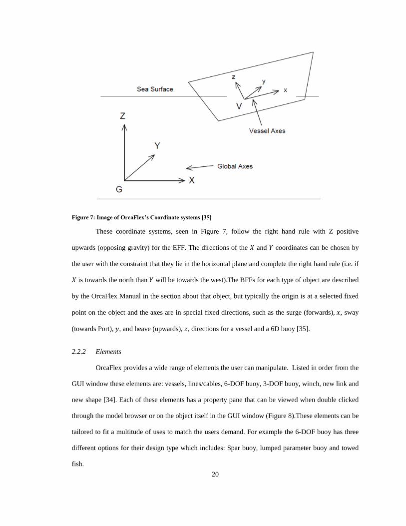
Figure 7: Image of OrcaFlex’s Coordinate systems [35]
These coordinate systems, seen in Figure 7, follow the right hand rule with Z positive
upwards (opposing gravity) for the EFF. The directions of the and coordinates can be chosen by
the user with the constraint that they lie in the horizontal plane and complete the right hand rule (i.e. if
is towards the north than will be towards the west).The BFFs for each type of object are described
by the OrcaFlex Manual in the section about that object, but typically the origin is at a selected fixed
point on the object and the axes are in special fixed directions, such as the surge (forwards), , sway
(towards Port), , and heave (upwards), , directions for a vessel and a 6D buoy [35].
2.2.2 Elements
OrcaFlex provides a wide range of elements the user can manipulate. Listed in order from the
GUI window these elements are: vessels, lines/cables, 6-DOF buoy, 3-DOF buoy, winch, new link and
new shape [34]. Each of these elements has a property pane that can be viewed when double clicked
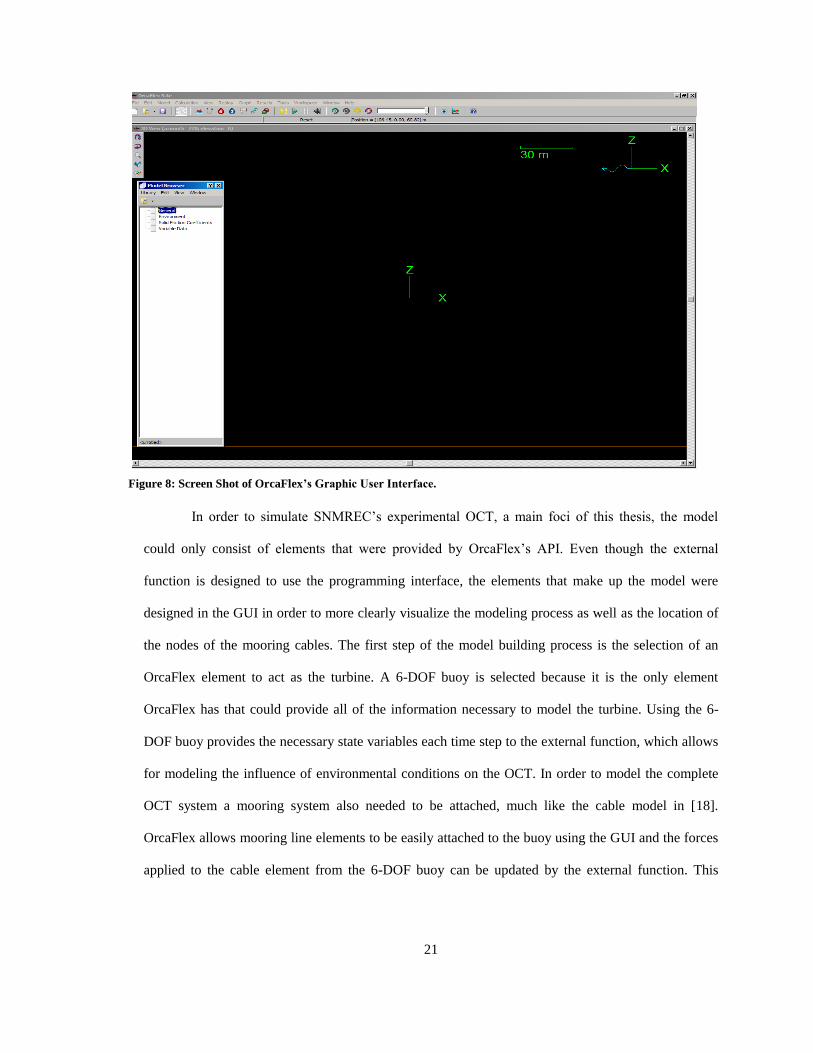
through the model browser or on the object itself in the GUI window (Figure 8).These elements can be
tailored to fit a multitude of uses to match the users demand. For example the 6-DOF buoy has three
different options for their design type which includes: Spar buoy, lumped parameter buoy and towed
fish.
21
In order to simulate SNMREC’s experimental OCT, a main foci of this thesis, the model
could only consist of elements that were provided by OrcaFlex’s API. Even though the external
function is designed to use the programming interface, the elements that make up the model were
designed in the GUI in order to more clearly visualize the modeling process as well as the location of
the nodes of the mooring cables. The first step of the model building process is the selection of an
OrcaFlex element to act as the turbine. A 6-DOF buoy is selected because it is the only element
OrcaFlex has that could provide all of the information necessary to model the turbine. Using the 6-
DOF buoy provides the necessary state variables each time step to the external function, which allows
for modeling the influence of environmental conditions on the OCT. In order to model the complete
OCT system a mooring system also needed to be attached, much like the cable model in [18].
OrcaFlex allows mooring line elements to be easily attached to the buoy using the GUI and the forces
applied to the cable element from the 6-DOF buoy can be updated by the external function. This
Figure 8: Screen Shot of OrcaFlex’s Graphic User Interface.
22
allows the thrust created by the turbine and the orientation of the turbine to affect the stress and
orientation of the mooring line and demonstrate the coupled effects.
2.2.3 External Functions
OrcaFlex can be used as a normal Windows Graphic User Interface (GUI) program (Figure 8)
or driven via a programming interface, or both [34]. The programming interface allows the user to
access and use a limited range of OrcaFlex's facilities to better suit individual user needs. The
implementation of external functions, which is done through a programming interface, provides the
means for users to create custom numeric models that suit their needs when the standard calculations
performed by OrcaFlex are inadequate. In order to incorporate the BEM model it is necessary to
receive variable updates each time step to accurately account for the momentum effects on the flow
and the blades, while incorporating the impact of the BEM calculated rotor forces into the response of
the mooring system. Knowing which values are utilized for these calculations is important because it
limits the types of elements that can be used in the GUI model, as well as the programming language
that the external function utilizes. In order to collect the necessary variables each time step the
program must either be written in Delphi or an object oriented C derivative, such as C or C++ [34].It
is important to note that the external function must be written in a way that allows for the creation of a
Dynamic-Link Library (.dll) file when built, so that external function could interact with OrcaFlex’s
Application Programming Interface (API).
2.2.3.1 API
In order to interface between different applications on any operating system it is crucial to be
familiar with the API of both applications. The API is essentially a list of the variables, routines, data
structures and object classes specific to each application. In this particular application, this means that
in order to access the variables that OrcaFlex updates, the external function must call from the data
structure that OrcaFlex stores them in using the same format that OrcaFlex uses to call them. For
example, OrcaFlex’s API stores the majority of its variables inside data structures for a wide array of
variable types and uses Long Pointers to Constant TCharSTRings (LPCTSTR) for most of its function
23
calls. This is due to the fact that Windows has moved away from the 2-bit character encoding and into
Unicode Transformation Format 16 bit (UTF-16) character encoding.
2.2.3.2 Variables
As previously mentioned the majority of the variables provided by OrcaFlex’s API are stored
within data structures, most of which are grouped by the element types described in subsection 2.2.2.
This allows variables of similar nature to be more easily accessed. In the case of the 6-DOF buoy that
is used in the simulation of SNMREC’s experimental OCT, the API provides access to a structure
denoted TBuoyInstantaneousCalculationData which holds the following variables [34]:
a position vector (buoy origin relative to the global origin),
orientation matrix (orientation of the buoy, relative to global axes),
vector velocity (velocity of the buoy origin relative to global),
vector angular velocity (angular velocity of the buoy relative to global),
vector for the wetted centroid location (local axes coordinates of the position of the
centroid of the wetted portion of the buoy),
vector for the undisturbed lumped fluid velocity at the wetted centroid position
(velocity of the fluid, current and wave combined, relative to global axes).
This fixed number of variables limits the calculations that can be performed in the external
functions and the numeric models that can be utilized. The undisturbed fluid velocity that is provided
by OrcaFlex combines the current velocity along with the wave velocity at the wetted centroid and
does not provide a profile for the swept water plane area.
2.2.4 Equations of motion
To properly account for the 7-DOFs, pitch, roll yaw, x, y, z and the rotor rotation, of an OCT
with a single rotor, that is modeled as having two rigid bodies allowed to rotate relative to each other
about a shaft at a pre-determined rotational velocity, it is important to document how OrcaFlex
24
handles the equations of motion for the 6-DOF buoy, which are being utilized when modeling the
OCT. OrcaFlex offers two dynamic integration schemes, Implicit and explicit, the latter is used for
this thesis so that a constant time step can be utilized. The explicit scheme utilizes the forward Euler’s
method for a fixed time step. To calculate the acceleration of a standard 6-DOF OrcaFlex element the
following equation is solved:
( ) ( ) ( ) ( ) (18)
where ( ) is the system inertial load, ( ) is the system damping load, ( ) is the system
stiffness load, ( ) is the external load, is the position and attitude vector, is the relative
linear and angular water velocity vector, is the linear and angular acceleration vector and is the
simulation time. This relationship is utilized to calculate the linear and angular accelerations of the 6-
DOF element, which are then numerically integrated to update the states of the system (Equation 17).
OrcaFlex considers the forces and moments from gravity, buoyancy, hydrodynamic and aerodynamic
drag, hydrodynamic added mass effects (which are calculated using the extended form of Morison’s
Equation with user defined coefficients), tension, shear, bending, torque, seabed reaction (including
friction) and contact forces with other objects [35].
To solve for the accelerations the linear and angular acceleration vector is factored out of the
inertial load matrix using Newton’s Second law:
( ) ( ) ( ) ( ) (19)
where ( ) is a 6x6 mass matrix comprised of the mass and moments of inertia, in the body fixed
coordinate system in the following form [36]:
25
( )
[
]
.
(20)
This is the local equation of motion used for each 6-DOF buoy and is not the same as Equation 16
since the acceleration is now an independent variable. In order to apply the forces and moments
calculated by the external function an addition term can be included in Equation 17 yielding:
( ) ( ) ( ) ( ) ( ) (21)
where ( ) is the force and moment vector calculated by the external function. In order to solve
this equation, all that is required is the inversion of the 6-DOF inertial matrix.
( )[ ( ) ( ) ( ) ( )] (22)
At the beginning of each time step this equation is solved for the acceleration of the 6-DOF buoy,
which is then integrated using Euler integration. At the end of each time step the position and
orientation are updated and the process repeats [35]. In this equation the moments are calculated about
the origin of the body fixed frame and the linear velocities are those of the origin of the body fixed
frame.
2.2.5 External Buoy Forces
To numerically model an OCT in OrcaFlex the external forces, ( ), on the turbine
utilized in the development of the OCT (chapter 3) are discussed here. The following equations are
used by the standard OrcaFlex external force equations available in the 6-DOF buoy element. These
include those induced by weight, buoyancy, hydrodynamic and aerodynamic drag, hydrodynamic
added mass effects (hydrodynamic drag and added mass are calculated using the extended form of
Morison’s Equation with user defined coefficients) [35]. In this thesis the force and moment vectors
are denoted as those from: weight, , buoyancy, , and the hydrodynamic interactions (both drag
26
and added mass) calculated using Morison’s Equation, ; which can be summed to calculate the net
external force and moment vector via:
( ) . (23)
Before delving into the force equations it is important to clarify how and where OrcaFlex
applies the calculated forces, when calculating the moments about the origin of the body fixed frame.
The 6-DOF buoy used to model the turbine is treated as a rigid body, with 3 translational and 3
rotational degrees of freedom. The hydrodynamic forces on 6-DOF buoys are calculated and applied
to the center of volume, where the center of volume is defined as:
( )
for a fully submerged buoy, (24)
where is the center of wetted volume, is the proportion that is wet and is the height of the
buoy. The moment on the 6-DOF buoy is then calculated using this force vector and the distance
vector between the center of volume and the origin of the body fixed coordinate system. It is
important to note that various components, including other 6-DOF can be rigidly linked to each other
to model the external forces and moments on complex shapes.
Weight
Calculation for weight forces and moments on 6-DOF buoys requires the user to define the
mass of the buoy and the distance vector from the origin to the center of mass. This is necessary for all
of the components that are rigidly linked together to create the modeled rigid system. This value needs
to be calculated before running the simulation as OrcaFlex provides the user with three input boxes in
the GUI window for each element that is defined, one for each of the directions in the body fixed
coordinate system. The first equation in this section addresses the weight of the 6-DOF buoy. The
weight force equation is represented by:
27
[ ] [
],
(25)
where is OrcaFlex’s transformation matrix, is the total buoy mass that is defined by the user
and is the gravitational constant. The moment caused by the weight force is therefore calculated
from:
[
] ,
(26)
where denotes the cross product.
Buoyancy
For the lumped buoy the buoyancy force is given by:
[ ] [
], (27)
where is the buoyancy, is the sea density and is the wetted volume. The buoyant force is then
applied vertically at the center of the wetted volume, . The moment created by the buoyant force is
therefore calculated from:
[
] .
(28)
where and represent the , and locations of the center of wetted volume.
Hydrodynamic Loads and Moments
In OrcaFlex the hydrodynamic loads are calculated and applied at each buoy’s and element’s center of
volume. These forces are calculated using the extended form of the Morrison Equation:
28
( )
⁄ | |, (29)
where is the fluid force vector, is the mass of the fluid displaced by the body, is the fluid
acceleration relative to the earth, is the added mass coefficient for the body, is the fluid
acceleration relative to the body, is the drag coefficient for the body, is the drag area and is the
relative water velocity vector. This equation is comprised inertial (portion on parentheses) and drag
components, with the inertial component including the Froude-Krylov force and added mass term.
These forces, and their distance from the origin, can be used to calculate the hydrodynamic moments
about the origin by:
[
] .
(30)
OrcaFlex elements can be set a fixed distances and orientations with respect to the origin of the body
fixed frame. Each individual body’s forces, and the moments about the common body fixed frame are
summed to calculate the net hydrodynamic forces and moments on the buoy.
.
29
3 OCT MODEL DEVELOPMENT
In this chapter the mathematical models utilized to predict OCT performance are presented.
This chapter focuses on the numerical calculations developed/implemented as part of this thesis, and
not those available as part of the standard OrcaFlex package (these are summarized in Section 2.2). It
also does not focus on the environmental conditions utilized to evaluate the numerically simulated
performance, as these are summarized with the individual analyses presented in Chapter 4. The first
section (Section 3.1) discusses the coordinate systems and kinematics used in modeling the motions of
an OCT, without referencing the force that causes the motion. The second section (Section 3.2)
provides a description of the equations of motion that are utilized in the overall behavior of the
system. The next section in this chapter (Section 3.3) describes how the hydrodynamic forces on the
on the OCT are calculated. The final section (Section 3.4) addresses specific properties of the
components of the OCT that is used for this thesis.
3.1 Coordinate Systems and Kinematics
The developed simulation will run within the OrcaFlex environment and therefore their EFF
and BFF coordinate systems will be utilized in the calculations (see section 2.2.1). Additionally, the
three coordinate systems utilized to calculate the forces on the rotor, presented later in this section,
will utilize the conventions described in [9]. These five coordinate systems are defined as: the earth
fixed coordinate system, ; the body fixed coordinate system, ; the momentum mesh coordinate
systems, , where ( ) indicates the referenced blade element radial location on mesh azimuth
angle grid point ( ) ; the shaft coordinate system, ; and the rotor blade coordinate systems,
,
where ( ) indicates the referenced blade element on the rotor blade ( ) . The ( ) symbol denotes all
potential variables that use the above listed superscripts. For the numerical simulations presented in
this thesis the earth fixed coordinate system is located at mean sea level; with the -axis oriented
30
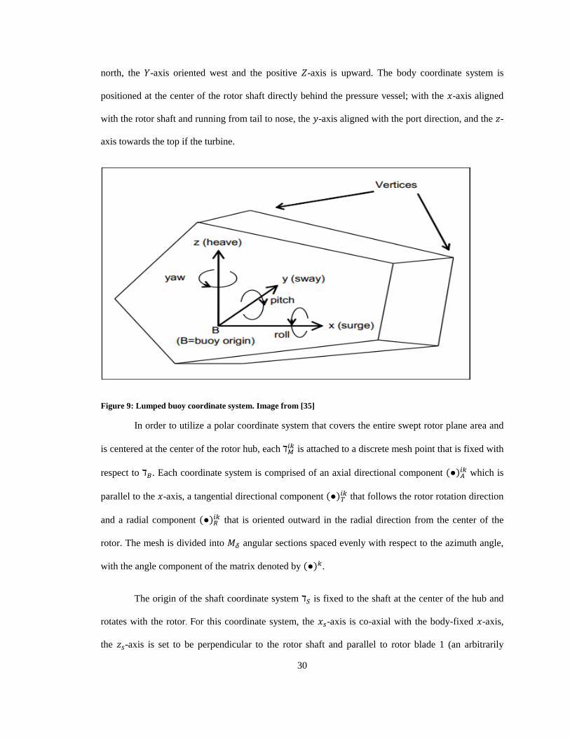
north, the -axis oriented west and the positive -axis is upward. The body coordinate system is
positioned at the center of the rotor shaft directly behind the pressure vessel; with the -axis aligned
with the rotor shaft and running from tail to nose, the -axis aligned with the port direction, and the -
axis towards the top if the turbine.
Figure 9: Lumped buoy coordinate system. Image from [35]
In order to utilize a polar coordinate system that covers the entire swept rotor plane area and
is centered at the center of the rotor hub, each is attached to a discrete mesh point that is fixed with
respect to . Each coordinate system is comprised of an axial directional component ( ) which is
parallel to the -axis, a tangential directional component ( ) that follows the rotor rotation direction
and a radial component ( ) that is oriented outward in the radial direction from the center of the
rotor. The mesh is divided into angular sections spaced evenly with respect to the azimuth angle,
with the angle component of the matrix denoted by ( ) .
The origin of the shaft coordinate system is fixed to the shaft at the center of the hub and
rotates with the rotor. For this coordinate system, the -axis is co-axial with the body-fixed -axis,
the -axis is set to be perpendicular to the rotor shaft and parallel to rotor blade 1 (an arbitrarily
31
chosen rotor blade), but extending from the shaft in the opposite direction and the -axis is aligned to
complete the right hand rule. In the final coordinate system, each
is fixed to the quarter cord line of
each of the discrete rotor blade sections and is comprised of the axial directional component ( )
which is aligned parallel to the -axis; a tangential directional component ( )
oriented in the
direction rotor rotation and a radial direction component ( )
that points outward in the radial
direction from the rotor’s center.
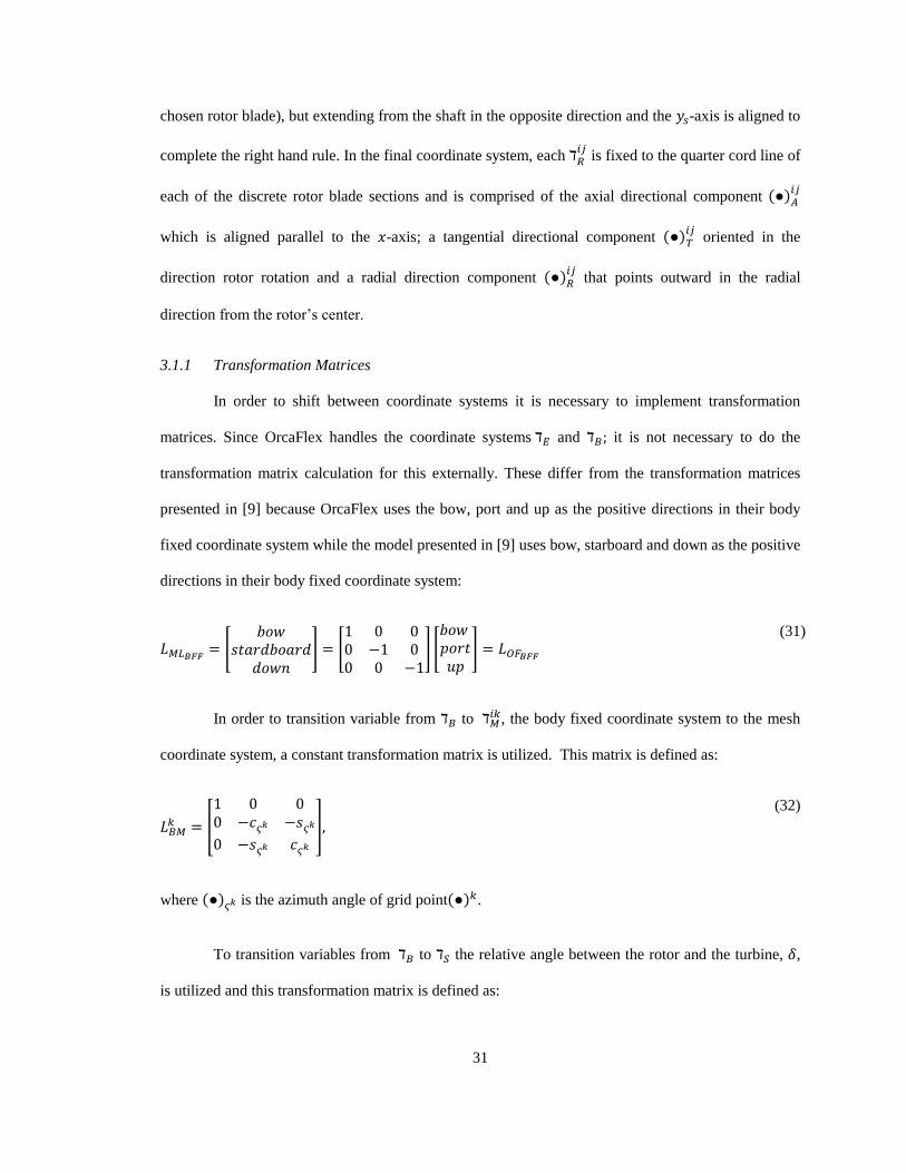
3.1.1 Transformation Matrices
In order to shift between coordinate systems it is necessary to implement transformation
matrices. Since OrcaFlex handles the coordinate systems and it is not necessary to do the
transformation matrix calculation for this externally. These differ from the transformation matrices
presented in [9] because OrcaFlex uses the bow, port and up as the positive directions in their body
fixed coordinate system while the model presented in [9] uses bow, starboard and down as the positive
directions in their body fixed coordinate system:
[
] [
] [
]
(31)
In order to transition variable from to , the body fixed coordinate system to the mesh
coordinate system, a constant transformation matrix is utilized. This matrix is defined as:
[
]
(32)
where ( ) is the azimuth angle of grid point( ) .
To transition variables from to the relative angle between the rotor and the turbine, ,
is utilized and this transformation matrix is defined as:
32
[
] (33)
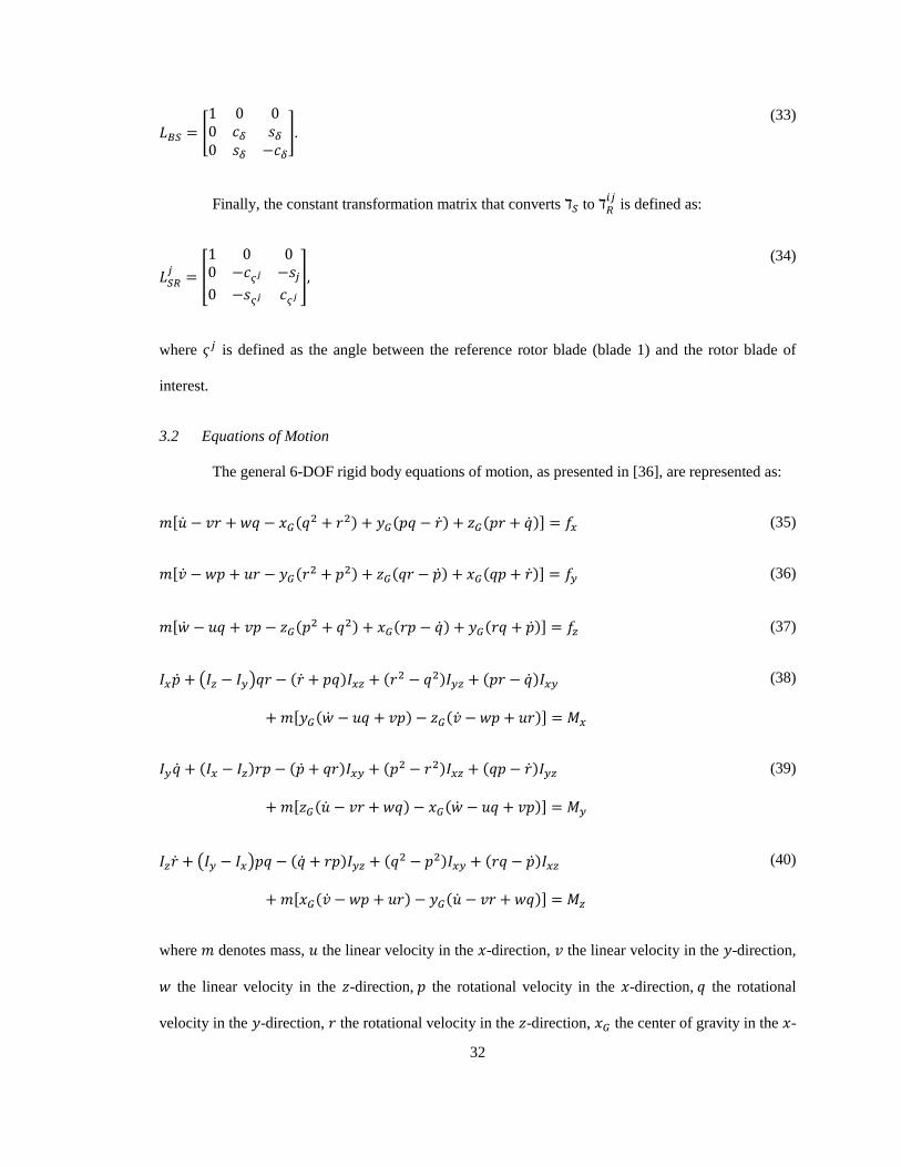
Finally, the constant transformation matrix that converts to
is defined as:
[
]
(34)
where is defined as the angle between the reference rotor blade (blade 1) and the rotor blade of
interest.
3.2 Equations of Motion
The general 6-DOF rigid body equations of motion, as presented in [36], are represented as:
[ ( ) ( ) ( )] (35)
[ ( ) ( ) ( )] (36)
[ ( ) ( ) ( )] (37)
( ) ( ) ( ) ( )
[ ( ) ( )]
(38)
( ) ( ) ( ) ( )
[ ( ) ( )]
(39)
( ) ( ) ( ) ( )
[ ( ) ( )]
(40)
where denotes mass, the linear velocity in the -direction, the linear velocity in the -direction,
the linear velocity in the -direction, the rotational velocity in the -direction, the rotational
velocity in the -direction, the rotational velocity in the -direction, the center of gravity in the -
33
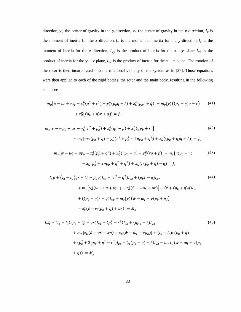
direction, the center of gravity in the -direction, the center of gravity in the -direction, is
the moment of inertia for the -direction, is the moment of inertia for the -direction, is the
moment of inertia for the -direction, is the product of inertia for the plane, is the
product of inertia for the plane, is the product of inertia for the plane. The rotation of
the rotor is then incorporated into the rotational velocity of the system as in [37]. Those equations
were then applied to each of the rigid bodies, the rotor and the main body, resulting in the following
equations:
[ ( )
( ) ( )] [
(( ) )
(( ) )]
(41)
[ (
) ( )
( )]
[ ( ) (
) (( ) )]
(42)
[ (
) ( )
( )] [ ( )
(
) ( ( ) )
(43)
( ) ( ) ( ) ( )
[ ( )
( )] ( ( ) )
(( ) ) [ ( ( ))
( ( ) )]
(44)
( ) ( ) ( ) ( )
[ ( ) ( )] ( ) ( )
( ) ( ( ) ) ( (
))
(45)
34
( ) ( ) ( ) ( )
[ ( )
( )] ( )( )
( ( )) ( )
( ( )
)
(46)
where is the mass of the body of the turbine, is the mass of the rotor, is the center of gravity
of the turbine body in the -direction, is the center of gravity of the turbine body in the -
direction, is the center of gravity of the turbine body in the -direction,
is the center of gravity
of the rotor in the -direction, is the center of gravity of the rotor in the -direction,
is the center
of gravity of the rotor in the -direction, is the rotational velocity of the turbine body and the
rotational velocity of the rotor, which are only valid at a constant RPM, that incorporates the
gyroscopic forces. The equations are finally in their full form for our system, now they will be reduced
to their simplest form using properties of the buoys, coordinate systems and assumptions. For these
calculations, the center of gravity was placed at the center of the rotor. With that assumption, , ,
, ,
and are all set equal to zero and the subscript and superscript can be dropped and
viewed as totals like: ,
and . Those assumptions lead to the development
of the following equations:
[ ( ) ( ) ( )] (47)
[ ( ) ( ) ( )] (48)
[ ( ) ( ) ( )] (49)
( ) ( ) ( ) ( )
[ ( ) ( )]
(50)
35
( ) ( ) ( ) ( )
[ ( ) ( )] (
)
(51)
( ) ( ) ( ) ( )
[ ( ) ( )] (
)
(52)
There is now an additional term on the right hand side of the equation that incorporates gyroscopic
forces created by the rotating turbine. OrcaFlex does not have a direct manner for handling this term
so the will be added to the ( ) , the forces and moments vector calculated by the external function
as a result of the rotor forces on the system, term calculated within the developed external function so
that the equations of motion discussed in Section 2.2.4 can be utilized without neglecting these
additional forces and moments.
3.3 Hydrodynamic Modeling
This section presents the approach utilized to calculate the hydrodynamic forces and moments
on the OCT system. Section 3.3.1 introduces the calculations utilized to calculate the forces on the
rotor, which are implemented into OrcaFlex using an external function. The Dynamic Wake model
(Section 3.3.1.1) is used to model the dynamic impact of the rotor on the incoming fluid. In the next
section (Section 3.3.2), the approach utilized to calculate the hydrodynamic forces and moments on
the remaining components using standard OrcaFlex elements is documented.
3.3.1 Rotor Modeling
In this section the mathematical rotor modeling techniques utilized in this thesis are discussed
in detail. This model utilizes an unsteady form of the BEM model to calculate the forces on the rotor
blades. The inputs into this rotor model are the OrcaFlex provided states (Section 2.2.3) and the
momentum states calculated from previous time steps. From these states the rotor model updates the
momentum states, which are utilized during the subsequent time step, and calculates and net
hydrodynamic forces and moments on the rotor, which are exported to OrcaFlex.
36
This model calculates the momentum loss in the flow field caused by the rotor forces in the
coordinate system. The impeded flow at each rotor blade element is then interpolated from the
adjacent radial points on this momentum mesh grid when calculating the relative water velocity
encountered by each rotor blade. Conversely, the flow reduction caused by the momentum loss is
calculated as if a blade element were at each momentum grid point. Therefore, both the actual rotor
forces and the rotor force calculations used in the momentum model are calculated each time step.
For each of the discrete radial location ( ) of both the rotor blade ( ) and azimuth angle of
the mesh grid ( ) , the angle of attack is calculated as a function of the axial
and
tangential
components of relative water velocity ,
[
]
.
These relative water velocities are calculated from:
(53)
( ). (54)
In this equation
is the effect of the device motions on the relative water velocity (from
Equations 22 and 23),
represents the combined velocity of the undisturbed free stream velocity
from both the waves and current (from Equations 25 and 26), and ( ) is the wake induced
velocity calculated from the previous time step. ( ) is initialized as a zeros matrix and is
then calculated using Equation 50 (Section 3.3.1.1) in subsequent time steps.
The
in Equation 21 is calculated from
[[
] [
] [
]] and
(55)
37
[[
] [
] [
]]
(56)
where and are the angular velocities about the and -axes imported from OrcaFlex and is sum
of the relative rotational velocity of the rotor about the -axis and the rotational velocity of the turbine
about the -axis imported from OrcaFlex:
(57)
The
term in Equation 21 is calculated from
[
]
[
] and
(58)
[
] [
]
(59)
where the undisturbed velocities imported from OrcaFlex in ( ) are functions of the
current profile, wave field, the turbine shaft location and time. The three scalar values, , and
, are imported from OrcaFlex each time step and are not dependent radial location ( ) , but are
made to be dimensionally consistent with the other matrices.
To calculate the hydrodynamic forces on the rotor, the angle of attack of each section of the
blade, is calculated by
(60)
where the relative flow angle in
is calculated from
38
(
) (61)
and is the blade section pitch angle, which is only a function of radial location.
Using the angles of attack calculated in Equation 26 with both the lift and drag coefficient
matrices, ( ) and
( ) respectively, the axial and tangential force coefficients are calculate
by:
( )
( ) and (62)
( )
( ). (63)
Using these coefficients axial and tangential loads on each of the blade sections are estimated by:
((
) (
) ) and
(64)
((
) (
) ),
(65)
where is the density of sea water and is the cord length at the center of center of section ( ) .
These forces are converted to by
[
]
[
]
(66)
and summed to calculate the total forces on the rotor
[
] ∑∑[
]
(67)
39
where ( ) is used in reference to the entirety of the rotor blade. Similarly, the hydrodynamic moment
from the rotor, with constant RPM, about the origin is calculated from
[
] ∑ ∑ [
] [
]
.
(68)
The forces calculated in Equation 33 and the moments calculated in 34, are summed with the
gyroscopic terms on the right had side of equation 41-46 to calculate the forces and moments exported
from the external function,
( )
[
]
[
(
)
(
) ]
(69)
to the OrcaFlex environment where they are summed with the forces and moments calculated directly
by OrcaFlex (Equation 20).
3.3.1.1 Dynamic Wake Model
This section describes the unsteady portion of the BEM model utilized to update the
calculated impact of the rotor on the incoming flow field. This requires calculating the quasi-static
impact of the rotor forces on the incoming flow field and then numerically converging the calculated
flow field to this constantly changing quasi-static value using a first order differential equation. This
section addresses the means by which a time delay is implemented and the effects the spinning rotor
blade has on the wake flowing past.
As mentioned earlier there is tip loss effect that has not been accounted for yet since the flow
past the coordinate system covers the entire swept rotor plane area, not accounting for the
individual blades. In order to make adjustments for the end effects of the rotor on the flow field
40
Prandtl’s tip loss factor, like that presented in Section 2.1.2.1, is applied. The tip loss factor used for
this simulation is calculated by
(
( )
( )),
(70)
where is the number of blades and is the total radius of the rotor.
For the time elapsed wake field, the updated axial induction factor from the previous time
step is defined as
( )
‖ ‖
(71)
Where ‖ ‖ denote the or Euclidean norm. Using this induction factor, the Glauert empirical
correction factor is calculated using
(
)
(72)
where .
The written external function allows device specific 3-D lift coefficients matrices, written as a
function of angle of attack and radial location, to be called at each time step. The lift coefficient
matrix, ( ) is calculated at each mesh node as a function of angle of attack, found in (27), in
order to obtain the lift per unit length,
(( )
(
) ), (73)
where is the radial distance from the rotor shaft elements and is the chord length at each radial
location.
41
The quasi-static wake field is now calculated in terms of its axial and tangential components
for time step :
( ) ( )
√(
( )) (
) (
)
(74)
( ) ( )
√(
( )) (
) (
)
(75)
where ( ) denotes that the utilized wake field is not corrected for the wake skew angle in Equation
38 and 39 and is the lift per unit length calculated in Equation 38.
Following the method provided by S. Oye, a filter is applied that consists of two first order
differential equations, Equations 26 and 27. These differential equations are solved analytically by
using intermediate wake variable vectors and as follows:
( )
( )
( )
(76)
( ) (
( ) ) (
)
(77)
( )
( ) ( ( )
( )) (78)
These equations are reliant on the constants and which are calculated by:
(79)
( )
(80)
42
( (
)
) (81)
This method is used because it calculates the impeded flow velocity for discrete locations over the
swept rotor plane area with a discrete mesh fixed with respect to the . To estimate the wake at the
blade elements, ( ), the wake is linearly interpolated between the nearest two azimuth angles in
the mesh grid ( ) for the same radial location:
( ) (
( ) ) (82)
A yaw model is included in this simulation that accounts for the relative yaw angle of the
rotor when calculating the impact of the rotor on the surrounding flow field. The method proposed by
Glauert is used to calculate this wake field corrected by
( ) ( )(
(
) ( ))
(83)
where is the wake skew angle defined as the angle between the current velocity in the wake and the
rotational axis of the rotor and is the angle where the blade is deepest into the wake. This wake
field is fed back into the relative flow speed calculations, Equation 21, in the following time step. The
skew angle in this equation is defined by
(‖∑(
) ∑(
)
‖
∑(
)
)
(84)
where ( ) denotes the four quadrant inverse tangent function and ( ) denotes that the skew
angle is assumed to be constant with the radius and is calculated at
⁄ = 7 as suggested by [17].
43
3.3.2 Streamlined Body Forces
The methodologies utilized to calculate the hydrodynamic forces on the streamline bodies will
follow those suggested by [20]. Below is a brief summary of this approach, including the fundamental
equations utilized to calculate the forces and associated moments. The streamline body forces that are
mathematically modeled using this approach include: two separate sections of the nacelle (the main
body of the turbine) and two Buoyancy Compensation Modules (BCM). The nacelle sections and
BCMs are modeled using standard OrcaFlex pipe elements. The drag forces and resulting moments
about the origin of the body fixed frame are calculated using the relative axial and tangential water
velocities calculated at the center of volume of each of these four bodies:
[
]
(85)
and
[ ] [
] (86)
where, is the mass of the fluid displaced by the body, is the fluid acceleration relative to the
earth, is the normal drag coefficient, is the coefficient of axial drag, is the frontal projected
area of the body, is the average diameter of the streamline body, is the length of the
streamline body, is the relative section speed through the water [8]. The forces and moment vectors
from these streamline bodies (two from the nacelle and one from each of the two BCMs) are summed
by OrcaFlex to calculate the total hydrodynamic force and moment vector:
[
],
(87)
which are summed with the other forces and moments according to (Equation 21) to calculate the total
force on the turbine.
44
3.4 Properties of SNMREC’s OCT
This section discusses the characteristics of the nearly neutrally buoyant SNMREC OCT
design that is utilized for creating the example results presented in this thesis. In order to compare the
OrcaFlex predictions with previously published results, the simulated system is based on the same
prototype design modeled by [20, 9]. The inertial, buoyancy, hydrodynamic, and geometric properties
of this turbine are presented in this section in the format necessary so that they can be directly
implemented into the external function and OrcaFlex 6-DOF buoy. These include the mass and inertial
system properties (Section 3.4.1) and hydrodynamic properties (Section 3.4.2).
3.4.1 Mass, Displace Volume and Inertial Properties
The mass, displaced volume and inertial properties of the modeled system are presented in
this section. These properties are derived from the nearly neutrally buoyant version of SNMREC’s
OCT presented in [9, 20]. The mass and displaced volumes of each object in this turbine design, as
well as the relative locations, are utilized for these calculations. The values in Table 3 are calculated
from this turbine design and presented in the form needed for implementation into OrcaFlex. Since
OrcaFlex allows users to implement the inertial properties directly into the program, these can be
directly calculated. However, OrcaFlex bases its buoyancy calculations on the volume and center of
volume of its various components and therefore needed to be calculated separately for the rotor, two
nacelle components, and two BCMs. Also, to allow for the placement of the BCMs to be easily
changed to optimize performance, the mass, volume and inertial properties of these are accounted for
separately from the rest of the system. The values in this table are given about the origin of the body
fixed frame, which is located at center of mass of the rotor.
45
Table 3: System mass, centers of Gravity, and mass moments with respect to the center of mass of the rotor and
the center of buoyancy that are plugged in to OrcaFlex(Products of inertia for x-y and y-z plane are zero due to
symmetry of OCT).
The values that are used by OrcaFlex (Table 3) correspond to an OCT system that that has the
mass and buoyancy characteristics that are presented in Table 4.
Table 4: Inertial characteristics of each component of the OCT system.
The turbine is almost neutrally buoyant with a net buoyant force of 302.82 N. The center of buoyancy
of this system is almost directly above the center of gravity, with the center of buoyancy 0.91 cm in
front of the center of gravity and 56.45 cm above the center of gravity.
3.4.2 Hydrodynamic Properties
The majority of the hydrodynamic system properties presented in this portion of thesis follow
those utilized by [9, 20]. In the OrcaFlex simulation used to model SNMREC’s OCT there are 3
Mass 1543.10 kg Length 2.34 m Length 0.508 m
Center of Gravity (x) 1.44 m Diameter 0.48 m Diameter 0.45 m
Center of Gravity (y) 0 m Density 162.89 kg/m3
Density 0.00 kg/m3
Center of Gravity (z) 0.15 m
Center of Buoyancy (x) 1.17 m Length 2.80 m X-Coordinate 3.03 m
Center of Buoyancy (y) 0.00 m Diameter 0.55 m Y-Coordinate 0.00 m
Center of Buoyancy (z) 0.04 m Density 0.00 kg/m3
Z-Coordinate -0.05 m
Mass Moment of Inertia (x) 337.51 kg-m2
Mass Moment of Inertia (y) 4435.60 kg-m2
Mass Moment of Inertia (z) 4187.00 kg-m2
Product of Inertia (x-z Plane) 408.47 kg-m2
Entire System (Not including BCMs)
Nacelle (Forward)
Nacelle (Aft)
Cable Attachment Point
BCMs
46
components that are hydrodynamically modeled. These modeled components are the rotor (section
3.5.2.1), the turbine nacelle (section 3.5.2.2) and the buoyancy compensation modules (section
3.5.2.3).
3.4.2.1 Rotor Hydrodynamic Properties
The hydrofoil shape of the numerically modeled rotor blades range in shape from
approximately NACA 4412 at the hub to NACA 4421 at the tip and transition through NACA 4415
and NACA 4418 between the hub and tip [9]. This OCT is designed to operate in a flow that is
approximately 2.0 ⁄ , with the rotor designed to operate near a Tip Speed Ratio (TSR) of roughly
4.0. XFoil, a tool designed by MIT, was used to calculate the 2D lift and drag coefficients for these
four airfoil shapes that are approximately evenly spaced from hub to tip by. The hydrofoil properties
are then entered into Airfoil Prep, a tool designed by NREL, to calculate the 3D lift and drag
coefficients for these four airfoil cross-sections. The method used to transition these four airfoil data
sets into lift and drag coefficients into a user specified number of evenly spaced airfoil cross-section
from hub to tip used a custom developed polynomial curve fitting routine, along with the sixty-four
predefined angles of attack, to create a set of second order polynomial equation (one for each pre-
defined angle of attack). These polynomials are then utilized, along with a linear interpolation routine,
to calculate the corresponding lift and drag coefficient for any angle of attack and radial location. The
lift and drag coefficients for 100 evenly spaced airfoil sections are plotted as a function of angle of
attack in Figure 10, with a zoomed in version of this figure presented in Figure 11.
47
Figure 10: 3D Lift and Drag Coefficient as angle a function of attack for all possible angles of attack
Figure 11: 3D Lift and Drag Coefficients as a function of angle of attack over the expected operating conditions
3.4.2.2 Turbine Nacelle
The hydrodynamic model used to estimate the forces on the turbine nacelle (the main body of
the turbine) is comprised two OrcaFlex pipe element that is separated into two distinct sections with
slightly different characteristics. The aft section of the nacelle, which extends in the negative
48
-direction behind the rotor, has a diameter of 0.508 m and a length of 0.508 m, while the forward
section of the nacelle has a diameter of 0.509 m and a length of 2.805 m [20].
OrcaFlex defines common values to act as default values when using the OrcaFlex bodies,
6-DOF buoys, lines/pipes, etc. For the majority of line or pipe elements, the forces at the end of the
pipes is typically neglected due to most of the implementations involve pipes of extensive length
which causes end drag to play minimal role when compared to skin drag. However, for our application
the length of the pipe is relatively short and therefore the end drag must be included. For this thesis the
default normal drag coefficients suggested by OrcaFlex for both of these sections are =1.2 is used.
The axial coefficients are a combination of end and skin drag for the back and front sections.
Assuming a skin drag coefficient of 0.008 and an end drag coefficient of 0.6 the coefficients
implemented into OrcaFlex and are calculated as follows:
(
) (
)
(88)
(
) (
)
(89)
where the skin drag coefficient is represented by , the end drag coefficient is , the resulting back
axial coefficient utilized by OrcaFlex is , and the resulting front end axial coefficient utilized by
OrcaFlex is . The added mass for the main body also uses the default value for a cylinder for both
axial ( ) and normal added mass (
) [20].
3.4.2.3 Buoyancy Compensation Modules
The buoyancy compensation modules on the numerically modeled version of the SNMREC
OCT are modeled as two separate ellipsoid bodies, each one evenly spaced with a center of volume
located 0.432 m, left and right of the rotor hub, 1.7 m above the rotor hub and 0.57 m forward of the
rotor plane area. For modeling simplicity, each of the BCM was given a constant diameter of 0.482 m
49
and length of 2.337 m in order to match the buoyancy of the actual specifications, which has the same
length of 2.337 m but has a varied diameter with a maximum of 0.53 m.
Since the BCM is modeled as a pipe in OrcaFlex as well, OrcaFlex’s default of for
normal drag coefficient was selected. The skin drag and end drag, are then used to calculate a
combined axial drag coefficient by:
(
) (
) , (90)
using a skin drag coefficient as 0.008 and end drag coefficient as 0.08 Each BCM, since they are
cylindrical in shape use OrcaFlex’s default properties for axial added mass and normal added
mass .
50
4 NUMERICAL RESULT
This chapter presents numerical estimates of OCT performance calculated using the
developed numerical modeling tools. Section 4.1 presents results calculated using the developed rotor
model alone, and compares these performance predictions with those calculated using published rotor
models. Section 4.2 presents numerical results calculated using the developed complete OCT
numerical system model attached to a mooring. These results highlight the utility of the numerical
model and provide predictions for the performance of a moored OCT.
4.1 Model Validation
This section presents the numerical validation of the developed BEM rotor model. The
selected operating scenarios are utilized to quantify the developed rotor model performance estimates
for steady state operations (4.1.1), the response of the momentum model to transient events (4.1.2) and
a wave environment (4.1.3). For these comparisons the developed numerical rotor model and the two
models utilized for validation, WT_Perf [38] (steady operations only) and Matlab [9] each used 100
elements for each blade. It is important to note that these in these comparisons Prandtl’s hub loss and
advanced brake-state models were disabled for WT_Perf, since these models were not utilized in the
other two numerical models.
4.1.1 Steady State
The steady operating condition analysis is the first stage of the validation process. In this
stage the coefficients of shaft power, torque and rotor thrust (drag) are analyzed, along with the shaft
power and restoring moment. These coefficients are calculated using the following non-dimensional
equations:
51
(91)
(92)
(93)
where is the coefficient of power, is the shaft power, is the density of water, is the swept
rotor plane area, is the free-stream velocity magnitude, is the coefficient of torque, is the shaft
torque, is the radius of the rotor blade, is the coefficient of thrust and is the thrust.
Two steady flow operating conditions are evaluated in this sub-section, which are utilized to
validate the developed rotor model against previously published numerical models. The first of these
conditions is a steady axial flow impacting a rotor rotating at a constant RPM. These results are
compared with the predicted steady state axial flow rotor performance calculated using the wind
turbine code WT_Perf [38], as well as a previously mentioned Matlab model [9] (sub-section 4.1.1.1).
The second operating condition quantifies the behavior of the OCT rotor for a steady but non-axial
flow. This off axis flow analysis compares the results for , power and the restoring moments about
the -axis when a progressive yaw is applied to the OCT of up to 30°, with results calculated using the
Matlab model.
4.1.1.1 Axial Flow
Axial flow testing allows for the prediction of the maximum shaft power output of the OCT,
as well as the relationship between TSR and power, torque, and thrust; which are important for
selecting the proper generator and gear box for maximum energy production, conducting heat
dissipation analyses, and estimating the potential energy production from OCTs. The coefficients of
power, torque and thrust are plotted against TSR in order to define the performance over the projected
operating range of tip speed ratios (Figure 12). In this figure the green lines represent Matlab based
52
predictions, black lines represent WT_Perf based predications, and red lines represent the results from
the developed numerical model. The data produced using the developed numerical model is also
presented in Table 4.
Figure 12: The predicted coefficients of power, thrust (drag) and torque using Matlab Model (green), WT_Perf
model (WTP)(black) and the OrcaFlex model (OF)(red *) as listed in the legend.
These results show that the predicted performance coefficients from the three numerical
models are very similar, especially at TSRs where maximum power is produced (from around 2-6).
The results for the maximum values calculated by the model developed in this thesis are ,
and occuring at the TSRs of 4.10, 3.50 and 2.00, respectively. The Matlab
model had maximums that were calculated to be at TSRs of 3.97, 3.65 and 2.05 which yield
, and , respectively. The WT_Perf model produced similar results with
53
maximum values of , and at the corresponding TSRs of 4.05,
3.65 and 2.08.
Table 5: This table shows the values for , and at a flow speed of 1.6 m⁄s calculated using the developed
rotor model.
4.1.1.2 Off axis flow
The off axis steady and homogeneous flow analysis characterizes OCT performance for the
likely scenario where the OCT is not precisely aligned with the oncoming flow. These time varying
forces that cyclically impact the blades each rotation can lead to fatigue failures or excite natural
frequencies of the system. For this evaluation the numerical predictions were made using an
undisturbed flow speed of 1.6 m/s. A rotor RPM of 41.74 was used in this analysis, resulting in a TSR
of 4.10 (corresponding to the maximum CP for an axial flow).
The relationship between mean shaft power and with respect to the off-axis angle is
presented in Figure 13.a and the relationship between restoring moment and off-axis angle is given in