INTERNATIONAL JOURNAL FOR NUMERICAL METHODS IN FLUIDSInt. J. Numer. Meth. Fluids 2016; 80:53–75Published online 24 July 2015 in Wiley Online Library (wileyonlinelibrary.com). DOI: 10.1002/fld.4071
Numerical simulations of bouncing jets
Andrea Bonito*,†, Jean-Luc Guermond and Sanghyun Lee
Department of Mathematics, Texas A&M University, College Station, Texas 77843-3368, USA
The ability of a jet of fluid to bounce on a free surface has been observed in different contexts.Thrasher et al. [1] designed an experiment where a jet of Newtonian fluid falls into a rotating vesselfilled with the same fluid. The authors investigated the conditions under which the jet bounces:nature of the fluid, jet diameter, and jet and bath velocities. We refer to [2] for experimental moviesillustrating this effect. Bouncing can also be observed in a stationary vessel provided the jet iscomposed of a non-Newtonian fluid. During the pouring process, a small heap of fluid forms andthe jet occasionally leaps upward from the heap (Figure 1). This is the so-called Kaye effect as firstobserved by [3] in 1963. About 13 years after this phenomenon was first mentioned in the literature,[4] revisited the experiment and suggested that the ability for the fluid to exhibit shear-thinningviscosity and elastic behavior are key ingredients for the bouncing to occur. Additional laboratoryexperiments performed by [5] and [6] lead the authors of each team to propose a list of propertiesthat the fluid should have for the Kaye effect to occur. The conclusions of these two papers disagreeon the requirement that the fluid be elastic and on the nature of the thin layer that separates the heapand the outgoing jet. It is argued in [5] that elastic properties are not necessary and that the thin layeris a shear layer, whereas it is argued in [6] that the fluid should have elastic properties and that thethin layer separating the heap from the bouncing jet is a layer of air. Recent experiments reported in[7] using a high speed camera unambiguously show that the jet slides on a lubricating layer of air.For completeness, we also refer to [8] for a thorough discussion on the ‘stable’ Kaye effect, wherethe jet falls against an inclined surface.
*Correspondence to: Andrea Bonito, Department of Mathematics, Texas A&M University, College Station, Texas 77843-3368, USA.
Figure 1. Experimental observation of the Kaye effect. (Left) The fluid starts to buckle producing a heap;(middle) a stream of liquid suddenly leaps outside the heap; (right) fully developed Kaye effect.
The objective of the present paper is to numerically revisit the Kaye effect. Our key finding isthat a thin air layer is always present between the bouncing jet and the rest of the fluid whether thefluid is Newtonian or not. Our numerical experiments suggest that the critical parameter for bounc-ing to occur is that the properties of fluid and the experimental conditions be such that a stable layerof air separating the jet and the ambient fluid can appear. This condition is met by setting the bathin motion for Newtonian fluids; it can also be met if the bath is stationary provided that the fluidis non-Newtonian and has shear-thinning viscosity. The numerical code that we use is based on amodeling of the fluid motion by the incompressible Navier–Stokes equations supplemented with asurface tension mechanism. The shear-thinning viscosity of the non-Newtonian fluids is assumedto follow a model by [9]. Elastic behaviors are not modeled. The numerical approximation of theresulting two-phase flow model is based on two solvers: one solving the Navier–Stokes equationsassuming that the fluid/air distribution is given, and the other keeping track of the motion of theinterface assuming that the transport velocity is given. The Navier–Stokes solver is based on a ver-sion of the projection method of [10] and [11] using a novel adaptive in time second-order backwarddifferentiation formula (BDF2) for the time discretization and adaptive finite elements for the spaceapproximation. The transport solver is based on a level set technique in the spirit of [12] to repre-sent the liquid/air interface. The level set is approximated in space by using adaptive finite elementsto accurately capture the aforementioned thin air layer, and the adaptive time stepping is carried outby using a third-order explicit Runge–Kutta technique. The transport of the level set function is sta-bilized using a novel ‘on the fly’ entropy residual method mathematically studied in [13] in a modelsetting, which guarantees an accurate representation of the free boundary.
The paper is organized as follows. The mathematical model is presented in Section 2. The numer-ical techniques to solve the Navier–Stokes equations and the transport equation for the level setfunction are described in Section 3. Various validation tests of the numerical algorithms and com-parisons with classical benchmark problems are reported in Section 4. Finally, we report numericalevidences of Newtonian and non-Newtonian bouncing jets in Section 5.
2. THE MATHEMATICAL MODEL
This section presents the mathematical models adopted to describe non-mixing two-phase fluidflows with capillary forces. Each fluid is assumed to be incompressible.
2.1. Two-phase flow system
Letƒ � Rd .d D 2; 3/ be an open and bounded computational domain with Lipschitz boundary @ƒand let Œ0; T � be the computational time interval, T > 0. The cavityƒ is filled with two non-mixingfluids undergoing some time-dependent motion, say fluid 1 and fluid 2. We denote by �C and ��
the open subsets of the space-time domain ƒ�Œ0; T � occupied by fluid 1 and fluid 2, respectively.We denote by �C; �C; ��; �� the density and dynamical viscosity of each fluid, respectively. Theinterface between the two fluids in the space-time domain is denoted † WD @�C \ @��, andthe normal to †, oriented from �C to ��, is denoted n†. The two space-time components of thevector field n† W † �! Rd � R are denoted n and n� , respectively. It is also useful to define�˙.t/ WD �˙\ .ƒ�¹tº/; that is, the sets�C.t/ and��.t/ are the regions occupied by fluid 1 and
fluid 2 at time t , respectively. We also introduce the interface †.t/ D @�C.t/ \ @��.t/; note thatn, as defined earlier, is the unit normal of †.t/ and it is oriented from �C.t/ to ��.t/. To facilitatethe modeling, we define global density and dynamical viscosity functions �; � W ƒ � Œ0; T � ! Rby setting �.x; t / D �˙ and �.x; t / D �˙ if .x; t / 2 �˙. The fluid velocity field u W ƒ � Œ0; T �!Rd , henceforth assumed to be continuous across †, and the pressure p W ƒ � Œ0; T � ! R aredefined globally and solve the incompressible Navier–Stokes equations in the distribution sense inthe space-time domain
�
�@
@tuC u � ru
�� 2div
��rSu
�Crp � ı†��n D �g in ƒ � .0; T �; (1a)
div.u/ D 0 in ƒ � .0; T �; (1b)
where rSu WD 12.ruCruT / is the strain rate tensor, g is the gravity field, and ı†��n is a singular
measure modeling the surface tension acting on †.t/. The distribution ı† is the Dirac measuresupported on †, the function � W † ! R is the total curvature of †.t/ (sum of the principalcurvatures) and � is the surface tension coefficient.
The system (1) is supplemented with initial and boundary conditions. The initial condition isu.x; 0/ D u0.x/ for all x 2 ƒ, where u0 is assumed to be a smooth divergence-free velocity field.The boundary @ƒ is decomposed into three non-overlapping components @ƒ WD �D [ �N [ �Swith �D \ �N D ;; �N \ �S D ;; �S \ �D D ;. Time-dependent decomposition could beconsidered but are not described here to avoid unnecessary technicalities. Given fN W �N ! Rd
and fD W �D ! Rd , we require that
�2�rSu � pI
�� D fN ; on �N � .0; T �; (2a)
u D fD; on �D � .0; T �; (2b)
u � � D 0;��2�rSu � pI
���� � D 0; on �S � .0; T �; (2c)
where � is the outward pointing unit normal on @ƒ and I is the d�d identity matrix. For simplicity,
we assume that the .d � 1/measures of �N [�S and �D are each strictly positive; otherwise, extraconstraints either on the velocity or on the pressure must be enforced.
Note that we could have formulated the conservation of momentum without invoking the singularmeasure modeling the surface tension by saying that (1a) holds in�C and�� (without the singularmeasure) and by additionally requiring that
Œu� D 0 and�2�rSu � pI
�n D ��n on †.t/; 8t 2 .0; T �; (3)
where Œ:� denotes the jump across †.t/ defined by Œv�.x/ WD lim��3y!x v.y/ � lim�C3z!x v.z/,that is, Œv�.x/ D v.x�/ � v.xC/, for all x 2 †.t/ and all v W ƒ! Rd or v W ƒ! Rd�d .
The interface †.t/ is assumed to be transported by the fluid particles. More precisely, let@�.ƒ�Œ0; T �/ be the part of the boundary of the space-time domain where the characteristicsgenerated by the field .u; 1/ enter, that is,
@�.ƒ � Œ0; T �/ WD ƒ � ¹0º [ ¹.x; t / 2 @ƒ � Œ0; T � ju.x; t / � � < 0º: (4)
We then define ¹x.P; t / 2 ƒ; t 2 ŒtP; T �; .P; tP/ 2 @�.ƒ� Œ0; T �/º to be the family of the character-istics generated by the velocity field u, that is, @
@tx.P; t / D u.x.P; t /; t/ with x.P; tP/ D P; .P; tP/ 2
@�.ƒ�Œ0; T �/ where tP is the time when the characteristics enters the space-time domainƒ� Œ0; T �at P. Let us now denote by †0 WD † \ @�.ƒ � Œ0; T �/ the location of the interface at the inflowboundary of the space-time domain, then we are going to assume in the entire paper that the velocityfield is smooth enough so that the following property holds
8x 2 †.t/; 9Š.P; tP/ 2 †0; x D x.P; t /; t > tP: (5)
2.2. Eulerian representation of the free boundary interface
A level set technique is used to keep track of the position of the time-dependent interface †.t/, seefor instance [12]. This method is recalled in Section 2.2.1. A typical problem arising when using alevel set method to describe interfaces is to guarantee the non-degeneracy of the representation. Wediscuss a reinitialization technique overcoming this issue in Section 2.2.2.
2.2.1. Level set representation. Let us define the so-called level function .x; t / W ƒ � Œ0; T �! Rso that
@
@t C u � r D 0 in ƒ � .0; T �; .P; tP/ D 0.P; tP/ on @�.ƒ � Œ0; T �/; (6)
where we assume that 0 is a smooth function satisfying the following properties:
@�˙ \ @�.ƒ � Œ0; T �/ D ¹.P; tP/ 2 @�.ƒ � Œ0; T �/ j ˙ 0.P; tP/ > 0º ; (7)
†0 WD † \ @�.ƒ � Œ0; T �/ D ¹.P; tP/ 2 @�.ƒ � Œ0; T �/ j0.P; tP/ D 0º : (8)
Note that this definition implies that †0 is the zero level set of 0. Upon introducing .P; t / WD.x.P; t /; t/ for all .P; tP/ 2 @�.ƒ � Œ0; T �/; t > tP, the definition of together with the definitionof the characteristics implies that @t .P; t / D 0 thereby proving that .x.P; t /; t/ D .P; t / D .P; tP/ D .x.P; tP/; tP/ D .P; tP/ D 0.P; tP/. This means that the value of .x.P; t /; t/ alongthe trajectory ¹x.P; tP/; t 2 ŒtP; T �º is constant; in particular, the sign of .x.P; t /; t/ does notchange. This leads us to adopt the following alternative definitions for �˙ and †.t/:
�˙ WD ¹.x; t / 2 ƒ�Œ0; T � j ˙ .x; t / > 0º; (9a)
†.t/ WD ¹x 2 ƒ j.x; t / D 0º: (9b)
The earlier characterizations will be used in the rest of the paper.To simplify the presentation, we are going to assume in the rest of the paper that there is �L � @ƒ
such that @�.ƒ � .0; T // D �L � .0; T /, that is, the inflow boundary for the level set equation istime independent. We then set L.P; t / D 0.P; t / for all P 2 �L, t 2 Œ0; T �, and we abuse thenotation by setting 0.P/ D 0.P; 0/ for all P 2 ƒ.
2.2.2. Reinitialization and cut-off function. A typical issue when dealing with level set representa-tion of interfaces is to guarantee that the manifold ¹x 2 ƒ j.x; t / D 0º is .d � 1/-dimensional,that is, we want to make sure that krk`2 > 0 in every small neighborhood of the zero level set,where k � k`2 is the Euclidean norm in Rd . In order to achieve this objective, we implement an ‘onthe fly’ reinitialization algorithm proposed in [14], which consists of replacing (6) by
@
@t�;ˇ C u � r�;ˇ D sign.�;ˇ /
�G.�;ˇ / � kr�;ˇk`2
�; (10)
where ; ˇ > 0 are parameters yet to be defined and G.�/; sign.�/ are defined by
G.´/ WD 1 ��´
ˇ
�2; sign.´/ WD
8<:
1; ´ > 0
�1; ´ < 00; j´j D 0:
(11)
The rationale for the new definition (10) is that the presence of the sign function in the right-handside implies that the zero level set of �;ˇ is the same as that of ; that is, the characterizations of�˙ and†.t/ are unchanged (9). Moreover, assuming that u is locally the velocity of a solid motion
and upon setting .P; t / D �;ˇ .x.P; t //, we have @@t D sign. /
Assuming that this eikonal equation has a steady-state solution 1 and denoting by †1 the zero-level set of this steady-state solution, the behavior of 1 in the vicinity of †1 is 1.P/ �ˇ tanh
�dist.†1;P/
ˇ
, because the solution to the following ODE W y0.´/ D 1 � .y.´/=ˇ/2 is
F.´/ WD ˇ tanh
�´
ˇ
�: (12)
Note that is close to 1 if is very large. In conclusion, the solution of (10) is such that�;ˇ .x; t / � ˇ tanh
�dist.†.t/;x/
ˇ
if is large enough, that is, krk`2 � 1 in any small neighbor-
hood of the zero level set. We are going to abuse the notation in the rest of the paper by droppingthe indices ; ˇ and by using instead of �;ˇ .
3. NUMERICAL METHOD
We discuss the approximations of the level set equation in Section 3.1 and that of the Navier–Stokessystem in Section 3.2. We consider a mesh sequence, ¹Thºh>0, and we assume that each mesh Th isa subdivision of ƒ made of disjoint elements K, that is, rectangles when d D 2 or cuboids whend D 3. We denote by E.Th/ the collection of interfaces and boundary faces (edge when d D 2 andfaces when d D 3). Each subdivision is assumed to exactly approximate the computational domain,that is, ƒ D [K2ThK, and to be consistent with the decomposition of the boundary, that is, thereexists EI .Th/ � E.Th/ for I 2 ¹D;N; S;Lº such that �I D [F 2EI .T /F . The diameter of anelementK 2 Th is denoted by hK I hK WD maxx;y2K jx�yj. The mesh sequence ¹Thºh>0 is assumedto be shape regular in the sense of Ciarlet. For any integer k > 1 and any K 2 Th, we denote byQk.K/ the space of scalar-valued multivariate polynomials over K of partial degree at most k. Thevector-valued version of Qk.K/ is denoted QQQk.K/. The index h is dropped in the rest of the paper,and we write T instead of Th when the context is unambiguous.
Regarding the time discretization, given an integer N > 2, we define a partition of the timeinterval 0 DW t0 < t1 < � � � < tN WD T and denote ıtn WD tn � tn�1 and tnC
12 WD tn C 1
2ıtnC1.
3.1. Numerical approximation of the level set system
The continuous finite element method used for the space approximation of level set Equation (10)is described in Section 3.1.1. We present in Sections 3.1.2 an entropy-residual technique that hasthe advantage of avoiding the spurious oscillations that would otherwise be generated by using anunstabilized Galerkin technique. The time stepping is performed by using an explicit strong stabilitypreserving (SSP) Runge–Kutta 3 (RK3) scheme as explained in Section 3.1.3.
3.1.1. Approximation in space. The space approximation of ˆ.�; t / of the level set function .�; t /solution to (10) is carried out by using continuous, piecewise linear polynomials subordinate to thesubdivision T . The associated finite element spaces are defined by
W .T / WD ¹W 2 C 0.ƒIR/ jW jK 2 Q1.K/; 8K 2 T º; (13)
W0.T / WD ¹W 2 C 0.ƒIR/ jW D 0 on �L; W jK 2 Q1.K/; 8K 2 T º; (14)
WL.T / WD ¹W 2 C 0.ƒIR/ jW D ˆL on �L; W jK 2 Q1.K/; 8K 2 T º; (15)
where ˆL.�; t / is a piecewise linear approximation of the inflow data L.�; t /. Assuming that thevelocity field u W ƒ � Œ0; T � �! Rd is known, the Galerkin approximation of (10) is formulatedas follows: Given ˆL and ˆ.�; 0/ D ˆ0, where ˆ0 2 W .T / is an approximation of the initialcondition 0, find ˆ 2 C1.Œ0; T �IWL.T // such thatZ
Figure 2. Graph of the level set function in the computational domain ƒ D .�1; 1/2 using the velocitygiven in (48) : (a) initial data: 0 is the characteristic function of the disk of radius 1 centered at
�12; 0�;
(b) no stabilization; (c) first-order stabilization with CLin D 0:1; and (d) entropy viscosity stabilization withCLin D 0:1 and CEnt D 0:1. Observe the spurious oscillations in panel (b) when no stabilization is applied.Both the first-order and the entropy viscosity solutions are free of oscillations, the latter being clearly more
accurate.
It is well known that the solution to the preceding system exhibits spurious oscillations in theregions where krˆk`2 is large. We address this issue in the next section.
3.1.2. Entropy residual stabilization. We describe in this section an entropy viscosity technique tostabilize the Galerkin formulation (16). This method has been introduced in [15], and we refer to[13] for a mathematical discussion on its stability properties. To motivate the discussion, we refer tothe panel (b) of Figure 2 showing the Galerkin approximation of the characteristic function of theunit disk, initially centered at .1
2; 0/, after one rotation about the origin.
The spurious oscillations are avoided by augmenting (16) with an artificial viscosity term wherethe viscosity is localized and chosen to be proportional to an entropy residual. To describe themethod and define an appropriate local ‘viscosity’, we recall that the following holds in thedistribution sense for any E 2 C1.ƒIR/:
@
@tE./C u�rE./ � sign./ .G.ˆ/ � krk`2/E 0./ D 0;
Consequently, it is reasonable to expect that the semi-discrete entropy residual
is a reliable indicator of the regularity of . This quantity should be of the order of the consis-tency error in the regions where is smooth, and it should be large in the region where the partialdifferential equation is not well solved. In our computations, we have chosen
E./ D jjp: (17)
The local so-called entropy viscosity is defined for any K 2 T by
�EntK .ˆ; u/ WD CEnth
2K
kREnt.ˆ; u/kL1.K/E.ˆ/ � 1jƒj
RƒE.ˆ/
L1.ƒ/
; (18)
where CEnt is an absolute constant. In the regions where is discontinuous (or has a very sharpgradient), the entropy viscosity as defined earlier may be too large and thereby introduce too much
diffusion, which in turn may severely limit the Courant-Friedrichs-Lewy (CFL) number when usingan explicit time stepping. In this case, a linear first-order viscosity is turned on instead
�LinK .ˆ; u/ D CLin
hK�
uC sign.ˆ/rˆ
krˆk`2
�L1.K/
; (19)
where CLin is an absolute constant. The justification for the definition of the local speed that isused to define the viscosity in (19) is that (10) can be rewritten @
@t C w�r D sign./G./,
where w D uC sign./ r�kr�k
`2. Combining the two viscosities yield the artificial viscosity �Stab W
ƒ � Œ0; T �! R defined on each K 2 T by
�Stab.ˆ; u/jK WD min.�LinK .ˆ; u/; �Ent
K .ˆ; u//: (20)
Going back to the space discretization, we modify (16) as follows: Look for ˆ 2C1.Œ0; T �IWL.T // so thatZ
ƒ
@
@tˆW D �
Zƒ
u�rˆW CZƒ
sign.ˆ/ .G.ˆ/ � krˆk`2/W �Zƒ
�Stab.ˆ; u/rˆ�rW (21)
for all W 2W0.T / and ˆ.�; 0/ D ˆ0.
3.1.3. Approximation in time. Before introducing the time discretization, we rewrite (21) asfollows: Z
ƒ
@
@tˆW D
Zƒ
L.ˆ; u/W �Zƒ
�Stab.ˆ; u/rˆ � rW; 8W 2W0.T ; t /; (22)
where L.ˆ; u/ WD �uC sign.ˆ/ .G.ˆ/ � krˆk`2/. Then we approximate time in the precedingnonlinear system of ODEs by using an explicit RK3 SSP scheme, for example, see [16, 17] for moredetails on SSP methods. We denote byˆk the approximation ofˆ.�; tk/; 0 6 k 6 N . Then, the timestepping proceeds as follows: Given ˆn, compute ˆ1; ˆ2; ˆ3 2 W.T / and ˆnC1 2WL.T / so that
.i/Zƒ
ˆ.1/W D
Zƒ
�ˆn C ıtnC1L.ˆn;un/
�W; 8W 2W .T /;
.ii/Zƒ
ˆ.2/W D
Zƒ
�3
4ˆn C
1
4ˆ.1/ C
1
4ıtnC1L.ˆ.1/;unC1/
�W
�
Zƒ
�Stab;nC1rˆ.1/ � rW; 8W 2W .T /;
.iii/Zƒ
ˆ.3/W D
Zƒ
�1
3ˆn C
2
3ˆ.2/ C
2
3ıtnC1L.ˆ.2/;unC
12 /
�W
�
Zƒ
�Stab;nC 12rˆ.2/ � rW; 8W 2W .T /;
(23)
and
ˆnC1.x; t / D²ˆ.3/.x/ when x 62 �L;upPhiL.x; tnC1/ when x 2 �L:
(24)
Using (20), the viscosities �Stab;nC1 and �Stab;nC 12 are defined to be equal to �Stab.ˆ.1/;unC1/ and�Stab
�ˆ.2/;unC
12
, respectively, where the residual REnt in the definition (18) of �Ent is evaluated
Remark 1 (‘On the Fly’ stabilization)Notice that following [13], no viscosity is added in the computation of ˆ.1/. In particular, the vis-cosities used within the time interval Œtn; tnC1� only depend on the values of ˆ and u on the sametime interval.
Remark 2 (Time-step criterion, stability, and convergence)We expect the scheme to be stable under the following CFL condition:
ıtnC1 6 CCFL minK2T
hK
ku .tnC1/C sign.ˆn/ rˆn
krˆnk`2kL1.K/
; (27)
for some sufficiently small but positive constant CCFL independent of ; T ; ıt; ˆ; and u. Refer forinstance to [13] for further details on the CFL condition. Moreover, it seems reasonable to expectthat only the entropy viscosity is active in the regions where is smooth; as a result, the CFLcondition implies that the first-order approximation of the time derivative in the evaluation of theentropy residuals, (25) and (26), does not affect the overall third-order approximation thanks to theh2K factor present in the definition of the viscosity (18). This conjecture is confirmed numerically inSection 4.2.3.2. Numerical approximation of the Navier–Stokes system
The space approximation of the velocity and pressure in the Navier–Stokes equations is carried outby using Taylor–Hood finite elements. The time discretization is carried out by using the BDF2.An incremental rotational pressure correction scheme is adopted to uncouple the velocity and thepressure. We refer to [18] for the convergence analysis of the method and to [19] for a review onprojection methods.
3.2.1. The space discretization. Let FD be a continuous, piecewise quadratic approximation of fDon �D . The finite element discretization of the velocity and the pressure is carried out by using thefollowing linear and affine spaces:
VVV 0.T / WD°
V 2 C 0�ƒIRd
jVj�D D 0; V � uj�S D 0; VjK 2QQQ2.K/; 8K 2 T
±; (28)
VVVD.T / WD°
V 2 C 0�ƒIRd
jVj�D D FD; V � uj�S D 0; VjK 2QQQ2.K/; 8K 2 T
±; (29)
M.T / WD®Q 2 C 0
�ƒ�! R jQjK 2 Q1.K/; 8K 2 T
¯: (30)
Upon setting U.0/ D U0, where U0 is a continuous, piecewise quadratic approximation of theinitial velocity u0 in VVVD.T /, the semi-discrete formulation of (1) consists of looking for U 2C1.Œ0; T �IVVVD.T // and P 2 C0.Œ0; T �IM.T / such that the following holds for every t 2 .0; T �:Z
ƒ
�
�@
@tUC .U � r/U
�� VC 2
Zƒ
��rSU W rSV
��
Zƒ
P divVCZƒ
Q divU
D
Zƒ
�g � VCZ�N
fN � VCZ†.t/
�� n � V; 8.V;Q/ 2 V0.T / �M.T /:(31)
3.2.2. Time discretization. The time discretization of (31) is performed by using the BDF2 andan incremental pressure correction scheme in rotational form introduced and studied in [20] todecouple the velocity and the pressure. In addition to the approximation of the initial condition
U0 mentioned earlier, the algorithm requires an approximation P0 2 M.T / of the initial pressurep.0/. We denote by Un, P n, and ‰n the approximations of U.�; tn/ and P.�; tn/ and the pressurecorrection, respectively.
The initialization step consists of setting: U0 D U0; P�1 D P 0 D P0 and ‰0 D 0. Then, givena new time step ıtnC1, given Un 2 VVVD.T /; ‰n 2 M.T /; and P n 2 M.T / and assuming forthe time being that �.tnC1/; �.tnC1/; and †.tnC1/ are also known (Section 3.4), the new fieldsUnC1 2 VVVD.T /; ‰nC1 2M.T / and P nC1 2M.T / are computed in three steps:
1 Velocity prediction: Find UnC1 2 VVVD.T / such thatZƒ
��tnC1
� ıBDF2
ıtnC1UnC1 � VC 2
Zƒ
��tnC1
� �rS
�UnC1
�W rSV
�C ST
�UnC1;V
�D �
Zƒ
��tnC1
� �.Un/? � rUn
�� VC
Zƒ
�P n C
4
3‰n �
1
3‰n�1
�div.V/
C
Zƒ
�nC1gnC1 CZ�N
fnC1N � VCZ†.tnC1/
��nC1 nnC1 � V; 8V 2 VVV 0.T /;
(32)
where
� the BDF2 approximation of the time derivative with variable time stepping is given by
@
@tU�x; tnC1
��ıBDF2
ıtnC1UnC1.x/
WD1
ıtnC1
1C 2�nC1
1C �nC1UnC1.x/ � .1C �nC1/Un.x/C
�2nC1
1C �nC1Un�1.x/
!;
where �lC1 WDıt lC1
ıt l.
� the extrapolated velocity .Un/? is defined by .Un/? WD Un C �n.Un � Un�1/;� as discussed in [21], the bilinear form ST W V .T / � V .T / ! R is added to control
the divergence of the velocity and to cope with variable time stepping and open boundaryconditions
ST .W;V/ WD Cstab
XK2T
ZK
��nC1 C �nC1khKWkL1.K/
�.r �W/.r � V/; (33)
where Cstab is an absolute constant.
2 Pressure-correction step: The pressure increment ‰nC1 2M.T / is determined by solving
Zƒ
r‰nC1rQ D �3minx2ƒ �
�tnC1
�2ıtnC1
Zƒ
div�UnC1
�Q; 8Q 2M.T /: (34)
3 Pressure update: The pressure P nC1 2M.T / is obtained by solvingZƒ
P nC1Q D
Zƒ
�P n C‰nC1
�Q � min
x2ƒ��tnC1
� Zƒ
div0�UnC1
�Q; 8Q 2M.T /: (35)
For stability purposes, we restrict the space and time discretization parameters to satisfy a CFLcondition
ıtnC1 6 CCFL1
2
minK2Th hKkUnkL1.ƒ/
; (36)
where CCFL is the same constant appearing in (27) and 12
minK2Th hK is the minimum distancebetween two Lagrange nodes using Q2 elements.
This section describes the approximation of the curvature termR†.tnC1/
��nC1 .nnC1 �V/ appearingin the first step of the projection method (32). We follow the method proposed in [22] (see also [23])using the work in [24]. This approach is based on the following representation of total curvature:
�n D r† � r†Id†;
where Id† is the identity mapping on† and, given any extension Qv of v in a neighborhood of†, thetangential gradient of v W †! Rd is defined by r†v WD r Qvj†.I � n˝ n/, see, for example, [25].Multiplying the preceding identity by a test function V and integrating by parts over † yieldsZ
†
��n � V D �Z†
�r†Id† W r†VCZ@†
�@� Id† � V; (37)
where � is the co-normal to † and @� is the derivative in the co-normal direction. In the presentcontext, the integral on @† vanishes because either † is a closed manifold or @� Id† D 0. Thisidentity together with the first-order prediction Id†.tnC1/ � Id†.tn/ C ıtnC1UnC1 of the interfaceevolution (5) gives a semi-implicit representation of the total curvatureZ
†.tnC1/
��nC1 .nnC1 � V/ D �Z†.tnC1/
r†.tnC1/Id†.tnC1/ W r†.tnC1/V
� �
Z†.tnC1/
r†.tnC1/Id†.tnC1/ W r†.tnC1/V
� ıtnC1Z†.tnC1/
�r†.tnC1/UnC1 W r†.tnC1/V:
One key benefit of this representation comes from the additional stabilizing termR†.tnC1/
�r†.tnC1/UnC1 W r†.tnC1/V, which we keep implicit in (32). The technicalities regarding the
approximation of this integral using the level set representation are detailed in Section 3.4.2 (45).
3.4. The coupled system
The two solvers described in Sections 3.1 and 3.2 earlier are sequentially combined. The flowchartof the resulting free boundary flow solver is shown in Figure 3. The remaining subsections ofSection 3.4 detail the coupling between the two solvers and other implementation technicalities.
3.4.1. Data for the level set solver (23)–(24). Following (23), givenˆn, an approximation of .tn/,the approximationˆnC1 of .tnC1/ requires the velocities u .tn/ ;u
�tnC
12
, and u
�tnC1
�. To avoid
an implicit coupling between the level set solver and the Navier-Stokes solver, these quantities arereplaced by second-order extrapolations using Un and Un�1:
u.tn/ � Un; u�tnC
12
� Un C
1
2
ıtnC1
ıtn
�Un � Un�1
�; and UnC1 � Un C
ıtnC1
ıtn
�Un � Un�1
�:
The sign.:/ function, which is used in the right-hand side of (10) to make sure that krk`2 isclose to 1 in a small neighborhood of † (i.e., on the fly reinitialization, see discussion following(11)), is redefined and replaced by:
signh.s/ D
8<:C1 if s > ˇ tanh.CS /;�1 if s < �ˇ tanh.CS /;0 otherwise,
where CS is an absolute constant. The thresholding in the preceding definition of the approximatesign function gives signh..x; t // D ˙1 whenever j�.x;t/j
ˇ> tanh.CS /, which is compatible with
the behavior �.x;t/ˇ� tanh
�dist.†.t/;x/
ˇ
that is expected for the level set function (12).
The parameter (‘reinitialization relative speed” in the language of [14]) is defined for t 2.tn; tnC1� by
D C�kUnkL1.ƒ/; K 2 T ; (39)
where C� is an absolute constant. This definition is motivated by the CFL condition (27). We referto [14] for further details.
3.4.2. Data for the Navier–Stokes solver. The definitions of the fields UnC1 and P nC1 in (32)–(35)invoke the values of the density field �nC1 and viscosity field �nC1. Once nC1 is computed, thesequantities are evaluated by using the following definitions
�nC1 D �C1CHh.ˆ
nC1/
2C ��
1 �Hh.ˆnC1/
2; (40)
�nC1 D �C1CHh.ˆ
nC1/
2C ��
1 �Hh.ˆnC1/
2; (41)
where �˙; �˙ are the density/viscosity in �˙, and Hh.:/ an approximation of the Heavisidefunction defined as follows:
Hh.s/ D
8̂<:̂
1 if s > ˇ tanh.CH /;�1 if s < �ˇ tanh.CH /;s
ˇ tanh.CH /otherwise;
(42)
where CH is an absolute constant, as suggested in [14]. Similarly to what we have carried out toapproximate the sign function, the preceding regularization is compatible with the behavior �.x;t/
ˇ�
tanh�
dist.†.t/;x/ˇ
that is expected for the level set function.
The approximation of the surface tension term in (32) is performed by following [23]. Let > 0, and consider the piecewise linear regularized Dirac measure supported on †.tnC1/, say ı� ,defined by
ı�.x/ WD
´1
�1 � dist.†;x/
�
if jdist.†; x/j < ;
0 otherwise:(43)
To account for the fact that we do not have access to the distance to the interface † but rather toan approximation of ˇ tanh
�dist.†;x/
ˇ
(Section 2.2.2), we rescale ı�.x/ as suggested in [26, 27] and
consider instead
ı�.x; ˆ/ D
´1
Q
�1 � ˆ.x/
Q�
krˆ.x/k`2 if jˆ.x/j < Q WD
krˆ.x/k`1
krˆ.x/k`2;
0 otherwise,(44)
where k � k`p is the `p-norm in Rd . In practice, we chose D ˇ tanh.CH / to be consistentwith the approximation of the Heaviside function (42). Using this approximate Dirac measure, theapproximation of the surface tension discussed in Section 3.3 becomes
Note that the preceding definitions correspond to approximating the normal vector n on†.tnC1/ by� rˆnC1
krˆnC1k`2
.
3.5. Adaptive mesh refinement
The experiments reported in [1, 6, 7] suggest that a critical feature of bouncing jets is the occurrenceof a thin layer between the jet and the rest of the fluid. These observations have led us to adopta mesh-refinement technique to describe accurately this thin layer. We propose here a refinementstrategy solely based on the position of the interface by increasing the mesh resolution around thezero level set of ˆ. More precisely, a cell K is refined if its generation count (the number of times acell from the initial subdivision has been refined to produce the current cell) is smaller than a givennumber Rmax and if
jˆ.xK ; t /j 6 ˇ tanh.CR/; (45)
where xK is the barycenter ofK and CR is an absolute constant. The purpose of the parameter Rmax
is to control the total number of cells. This refinement strategy leads to subdivisions where all theelements crossing the zero level set ofˆ have the same diameter (up to a constant only depending onthe coarse mesh). The parameter CR controls the distance to the interface below which refinementoccurs. In fact, recalling that using the filter (12) implies that .x; t / � ˇ tanh
�dist.†.t/;x/
ˇ
if is
large enough, we expect the refinement criteria (45) to be active whenever dist.†.t/; x/ 6 CRˇ.Note that (45) is compatible with (38) and (42). The subdivisions are carried out with at most onehanging node per face, see, for example, Bonito and Nochetto [28, Section 6.3]. A cell is coarsen ifit satisfies the following three conditions: its generation count is positive;
jˆ.xK ; t /j > ˇ tanh.CC /; (46)
where CC > CR is an absolute constant; and if once coarsened, the resulting subdivision does nothave more than one hanging node per face. We refer to the documentation of the deal.II library forfurther details [29].
4. NUMERICAL VALIDATIONS
The algorithm presented in the previous sections has been implemented using the deal.II finiteelement library described in [29, 30]. Parallelism is handled by using the message passing inter-face library [31]. The subdivision and mesh distribution is carried out by using the p4est libraryfrom [32].
The rest of this section illustrates and evaluates the performance of the preceding algorithm.We start in Section 4.1 by specifying all the numerical constants required by the algorithm. Thevalidation of the transport code for solving the level set equation is carried out in Section 4.2. Thevalidation of the two-phase fluid system is performed in Section 4.3.
4.1. Numerical parameters
Our algorithm involves several numerical parameters. In this section, we briefly recall their meaning,where they appear, and we specify the value of each of them. Unless specified otherwise, thesevalues are fixed for this entire section. Except for Section 4.2, the time discretization parameter isalways chosen according to (27).
A complete list of all the parameters is shown in Table I. The parameter ˇ determining the widthof the hyperbolic tangent filter (12) is defined to be ˇ D minK2T hK . This definition is used inthe expression of the hyperbolic tangent filter (12), in the threshold of the approximate Heavisidefunction (42) and the approximate sign function (38), and in the refinement strategy, (45) and (46).In particular, the expected number of elements in the transition layer separating the two phases is2CR D 4 (Section 3.5).
4.2. Transport of the level set
4.2.1. Convergence tests. The consistency of the algorithm for the approximation of the level setEquations (23) and (24) is a priori third-order in time and space. To evaluate whether this is indeedthe case, we solve the linear transport equation in the unit squareƒ D .0; 1/2 using the velocity field
u.x; y; t/ WD�� sin2.�x/ sin.2�y/ cos.�t=0:1/
sin2.�y/ sin.2�x/ cos.�t=0:1/
�:
This flow is time periodic of period 1, which implies that .x; 0:2/ D 0.x/, for all x 2 ƒ. Theinitial level set function is chosen to be the signed distance to the line of equation y D 0:5:
0.x; y/ D y � 0:5: (47)
The errors are evaluated at t D 0:2. Three different scenarios are considered: (i) no stabilization andno reinitialization; (ii) entropy viscosity stabilization and no reinitialization; (iii) entropy viscosityand reinitialization, that is, the complete algorithm. Except for ˇ, the values of the numerical param-eters are given in Table I. We consider four computations carried out on four uniform meshes
Table I. Description and values of the numerical parameters.
Table II. Single vortex test case: L2-norm of error and observed convergence rates for eachscenario after one period for different time discretization resolutions.
(i) Runge–Kutta 3 (RK3) Galerkin algorithm; (ii) RK3 algorithm with entropy viscosity; (iii) RK3with entropy viscosity and reinitialization. Third-order convergence rate is observed in all scenarios.
Figure 4. (a) Initial level set: the dark region corresponds to 0 > 0; (b)–(e) comparison of the graphs of theexact (solid line) and approximate (dashed line) level set functions along the line of equation x D 0:5 afterone revolution: (b) without stabilization and reinitialization .CLin D CEnt D C� D 0/; (c) with first-orderlinear stabilization, CLin D 0:1; (d) with entropy residual stabilization, CLin D 0:1 and CEnt D 0:1; and (e)with entropy residual stabilization and reinitialization, C� D 0:01. The transport without stabilization of thenearly discontinuous level set function yields spurious oscillations. These oscillations are removed by thelinear viscosity at the expense of large numerical diffusion. The numerical diffusion is minimized by turningon the entropy residual term. Finally, adding the reinitialization allows to nearly recover the exact profile.
with constant time steps. The mesh size and the time step are divided by 2 each time. The meshesare composed of 1089, 4225, 16,64, and 66,049 Q2 degree of freedoms. The space discretization ischosen fine enough not to influence the time error. We report in Table II, the errors kˆN �0kL2.ƒ/for the three scenarios and the observed rates of convergence. Note that the reinitialization is turnedon in scenario (iii), which implies that the exact solution at t D 0:2 is not 0 anymore; we mustinstead compare ˆN with ˇ tanh
��0.x;y/ˇ
. In this particular case, we keep ˇ constant to ascertain
the third-order consistency of the algorithm; we set ˇ D 0:0203125.
4.2.2. Rotation of a circular level set: Effect of different viscosities and reinitialization. In this testcase, the initial data for the level set are the hyperbolic tangent filter applied to the distance to thecircle centered at (0.5,0) and of radius 0.25
0.x; y/ WD ˇ tanh
0:25 � ..x � 0:5/2 C y2/
12
ˇ
!; .x; y/ 2 ƒ WD .�1; 1/2;
see Figure 4(a). The level set is transported by using the solid rotation velocity field:
u.x; y/ WD��yx
�: (48)
The computation is carried out with the adaptive algorithm described in Section 3.5 usingRmax D2. The initial mesh is uniform with hK D 0:015625 for all K 2 T . The resulting time-dependentmesh is such that minT2T hK � 0:00390625, that is, we set ˇ D 0:00390625. The values of theother numerical constants are provided in Table I. The time step ıt is chosen to be uniform and equalto ��10�3. We compare the initial level set with its approximation after one revolution. Figure 4(b)–(e) illustrates the benefits of using the entropy stabilization and the reinitialization technique bycomparing the graphs of the exact and approximate level set functions along the line of equationx D 0:5 after one revolution.
4.2.3. 3D slotted disk: long-time behavior. A typical benchmark for the transport of a level setfunction is the so-called Zalesak disk documented in [33]. We consider in this section the three-dimensional version thereof. The computational domain is ƒ WD .0; 1/3. The initial level set is thecharacteristic function of a slotted sphere centered at (0.5,0.75,0.5) with a radius of 0.15. The width,height, and depth of the slot are 0.0375, 0.15, and 0.3 respectively (Figure 5(a)). The initial profileis transported by using the following velocity field:
Figure 5. Rotating slotted three-dimensional sphere. From left to right, the dark regions correspond to ˆ >0 after 0,1,2,3,4, and 5 full rotations. Oscillations and numerical diffusion are controlled by the entropy
viscosity as well as the reinitialization algorithm.
Figure 6. Iso-contour ˆ D 0 in the plane ´ D 0: (A) initial data; (B) after one rotation; (C) after three rota-tions; and (D) after five rotations. Numerical diffusion is observed but is greatly minimized by the entropy
viscosity and reinitialization techniques.
The time step is chosen to be uniform ıt D � � 10�3. The initial subdivision is composed ofcells of diameter 0.015625. The adaptive mesh refinement technique described in Section 3.5 is usedwith Rmax D 2; the minimum mesh size is minK2T hK D 0:00390625. The numerical constantsare given in Table I. The computation is performed until the slotted sphere has undergone five fullrevolutions. The iso-surface ˆ D 0 is shown in Figure 5 after each of the five periods. Oscillationsand numerical diffusion are controlled by the entropy viscosity and the reinitialization algorithm. Acloser look at the slotted region is provided in Figure 6.
4.2.4. Single vortex: large deformations. The single vortex problem consists of the deformationof a sphere by a time-periodic incompressible vortex-like flow. The computational domain is ƒ D.0; 1/3, and the time-periodic velocity field is defined by
u.x; y; t/ WD
0@� sin2.�x/ sin.2�y/ cos.�t=4/
sin2.�y/ sin.2�x/ cos.�t=4/0
1A : (50)
The initial level set is given by
0.x/ WD ˇ tanh
�dist.S; x/
ˇ
�; (51)
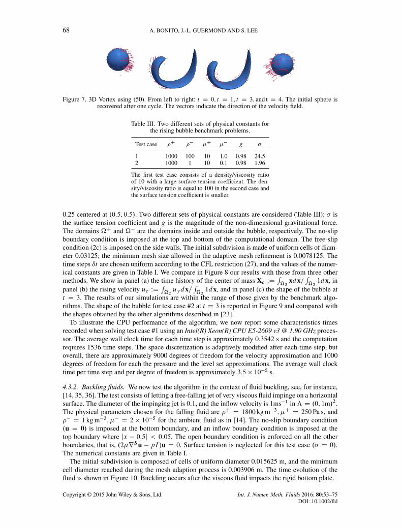
where S is the sphere centered at (0.5,0.75,0.5) of radius of 0.15. The field 0 is a regularizedversion of the distance function using the tanh cut-off filter (12). The divergence-free velocity fieldseverely deforms the level set until t D 2 and returns it to its initial shape at t D 4. The time stepis chosen to be uniform ıt D 0:001 and the final time is t D 4 (one cycle). The initial subdivisionis made of uniform cells of diameter 0.015625; the minimum mesh size allowed in the adaptivemesh refinement is 0.00390625. The numerical constants are given in Table I. Figure 7 shows theiso-contour ˆ D 0 at different times. The undeformed sphere is recovered after one cycle.
4.3. Two-phase flows
4.3.1. Rising bubble: surface tension benchmark. We start the validation of the two-phase flow sys-tem with the Rising bubble benchmark problem, see, for example, [23]. The computational domainisƒ D .0; 1/� .0; 2/, the initial data 0 are the characteristic function of a circular bubble of radius
Figure 7. 3D Vortex using (50). From left to right: t D 0; t D 1; t D 3; and t D 4. The initial sphere isrecovered after one cycle. The vectors indicate the direction of the velocity field.
Table III. Two different sets of physical constants forthe rising bubble benchmark problems.
The first test case consists of a density/viscosity ratioof 10 with a large surface tension coefficient. The den-sity/viscosity ratio is equal to 100 in the second case andthe surface tension coefficient is smaller.
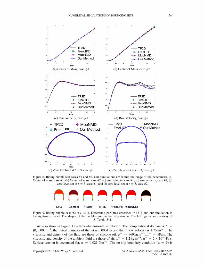
0.25 centered at .0:5; 0:5/. Two different sets of physical constants are considered (Table III); � isthe surface tension coefficient and g is the magnitude of the non-dimensional gravitational force.The domains �C and �� are the domains inside and outside the bubble, respectively. The no-slipboundary condition is imposed at the top and bottom of the computational domain. The free-slipcondition (2c) is imposed on the side walls. The initial subdivision is made of uniform cells of diam-eter 0.03125; the minimum mesh size allowed in the adaptive mesh refinement is 0.0078125. Thetime steps ıt are chosen uniform according to the CFL restriction (27), and the values of the numer-ical constants are given in Table I. We compare in Figure 8 our results with those from three othermethods. We show in panel (a) the time history of the center of mass Xc WD
R�2
xdx=R�21dx, in
panel (b) the rising velocity uc WDR�2uydx=
R�21dx, and in panel (c) the shape of the bubble at
t D 3. The results of our simulations are within the range of those given by the benchmark algo-rithms. The shape of the bubble for test case #2 at t D 3 is reported in Figure 9 and compared withthe shapes obtained by the other algorithms described in [23].
To illustrate the CPU performance of the algorithm, we now report some characteristics timesrecorded when solving test case #1 using an Intel(R) Xeon(R) CPU E5-2609 v3 @ 1.90 GHz proces-sor. The average wall clock time for each time step is approximately 0.3542 s and the computationrequires 1536 time steps. The space discretization is adaptively modified after each time step, butoverall, there are approximately 9000 degrees of freedom for the velocity approximation and 1000degrees of freedom for each the pressure and the level set approximations. The average wall clocktime per time step and per degree of freedom is approximately 3:5 � 10�5 s.
4.3.2. Buckling fluids. We now test the algorithm in the context of fluid buckling, see, for instance,[14, 35, 36]. The test consists of letting a free-falling jet of very viscous fluid impinge on a horizontalsurface. The diameter of the impinging jet is 0:1, and the inflow velocity is 1ms�1 inƒ D .0; 1m/2.The physical parameters chosen for the falling fluid are �C D 1800 kg m�3; �C D 250Pa s; and�� D 1 kg m�3; �� D 2 � 10�5 for the ambient fluid as in [14]. The no-slip boundary condition.u D 0/ is imposed at the bottom boundary, and an inflow boundary condition is imposed at thetop boundary where jx � 0:5j < 0:05. The open boundary condition is enforced on all the otherboundaries, that is, .2�rSu � pI/u D 0. Surface tension is neglected for this test case .� D 0/.The numerical constants are given in Table I.
The initial subdivision is composed of cells of uniform diameter 0.015625 m, and the minimumcell diameter reached during the mesh adaption process is 0.003906 m. The time evolution of thefluid is shown in Figure 10. Buckling occurs after the viscous fluid impacts the rigid bottom plate.
Figure 8. Rising bubble test cases #1 and #2. Our simulations are within the range of the benchmark. (a)Center of mass, case #1, (b) Center of mass, case #2, (c) rise velocity, case #1, (d) rise velocity, case #2, (e)
zero level set at t D 3, case #1, and (f) zero level set at t D 3, case #2.
Figure 9. Rising bubble case #2 at t D 3. Different algorithms described in [23], and our simulation inthe right-most panel. The shapes of the bubbles are qualitatively similar. The left figures are courtesy of
S. Turek [34].
We also show in Figure 11 a three-dimensional simulation. The computational domain is ƒ D.0; 0:008m/3, the initial diameter of the jet is 0.0004 m and the inflow velocity is 1:75ms�1. Theviscosity and density of the fluid are those of silicone oil: �C D 960 kg m�3; �C D 5Pa s. Theviscosity and density of the ambient fluid are those of air: �� D 1:2 kg m�3; �� D 2 � 10�5Pa s.Surface tension is accounted for, � D 0:021 Nm�1. The no-slip boundary condition .u D 0/ is
Figure 10. (From left to right) Time evolution of a jet of very viscous liquid inside a cavity filled with air.Buckling occurs when the liquid hits the floor.
Figure 11. (a)–(e) Time evolution of a three-dimensional jet of Silicone oil falling in a cavity filled with airat time (a) t D 0:00501, (b) t D 0:0209, (c) t D 0:031, and (d) t D 0:048998 s. For comparison, (e) showsthe shape of the Silicone oil jet obtained in laboratory with the same physical conditions. Our numerical
simulations are qualitatively in agreement with the physical experiment.
imposed at the bottom of the box. The inflow boundary is the diskp.x � 0:004/2 C .y � 0:004/2 <
0:0002 at the top boundary (´ D 0:008). Open boundary conditions .2�rSu � pI/� D 0 areapplied on the rest of the boundary. The results are obtained with adaptive mesh refinement withthe minimum cell diameter 6:25 � 10�5. The time steps follow the CFL restriction (27) and thenumerical constants are given in Table I.
5. NUMERICAL SIMULATIONS OF BOUNCING JETS
We now use our algorithm to predict the bouncing effect of jets of Newtonian (Section 5.1) andnon-Newtonian (Section 5.2) fluids. In both cases, the formation of a thin layer of air between thejet and the bulk of the fluid is a critical ingredient to observe the bouncing effect. The adaptive meshrefinement strategy adopted in our algorithm allows to capture this thin layer with a reasonablenumber of degrees of freedom.
5.1. Two-dimensional Newtonian bouncing jets
We start with a Newtonian fluid falling into a translating bath as in the experiment proposed in[1]. The fluid is a silicone oil with viscosity �C D 0:25 Pa s and density �C D 960 kg m�3.The ambient fluid is air: �� D 1:2 kg m�3 and �� D 2 � 10�5 Pa s. The computational domainis ƒ WD .0; 0:04 cm/ � .0; 0:06 cm/. The radius of the incoming jet is 0.25 cm; its velocity isu D .0;�5 cm s�1/ on ¹.x; y/ 2 @ƒ W y D 4; jx�0:01j < 0:0025º. The region ¹.x; y/ 2 ƒ W 0 <y < 0:02º is filled by the same fluid, called the ‘bath’, and it moves to the right with a horizontalvelocity VB to be specified later. Slip-boundary condition (2c) is imposed at the bottom of the cavity,and the open boundary condition .2�rSu � pI/u D 0 is applied to the rest of the boundary
¹.x; y/ 2 @ƒ W y D 4; jx � 0:01j > 0:0025º[¹.x; y/ 2 @ƒ W x D 0; y > 0:02º [ ¹.x; y/ 2 @ƒ W x D 0:04º:
The values of the numerical constants are those given in Table I. The minimum cell diameter result-ing from the adaptive mesh refinement strategy is 7:8125 � 10�5 cm. The time steps are chosen tosatisfy the CFL restriction (27).
As already noted in [1], there is a range of velocities for which bouncing occurs, and the jet slidesalong the surface of the bath when the horizontal velocity of the bath is too high. This is illustrated
Figure 12. Newtonian bouncing jet (from left to right). The white arrow indicates the translation direction ofthe bath. (a) Bath velocity VB D 8 cm s�1 and surface tension coefficient � D 21mN m�1; the incomingjet bounces away from the bath, and we observe the apparition of an air layer between the jet and the bath.(b) Bath velocity VB D 25 cm s�1 and surface tension coefficient � D 21mN m�1; in this case, the bathvelocity is too large and the jet slides along the bath surface; (c) bath velocity VB D 8 cm s�1 but without
surface tension � D 0mN m�1; compare with (a).
in Figure 12(a) and (b): the jet bounces when VB D 8 cm s�1 (Figure 12(a)), but it slides whenVB D 25 cm s�1 (Figure 12(b)). Note that it is necessary to include the surface tension to keepthe jet stable after impinging on the free surface as illustrated in Figure 12(c) where a simulationwithout surface tension is presented. Observe finally that all our numerical simulations show that athin layer of air is formed between the jet and the bath each time the jet bounces.
5.2. Kaye effect
The Kaye effect is the name given to the bouncing jet phenomenon when the bath is stationary. Thiseffect has been observed to occur only with non-Newtonian fluids. It is now recognized that shear-thinning viscosity is a critical component of the Kaye effects, see, for example, [4–6]. Following[5], we adopt the model of [9] in the rest of the paper
�.�/ D �1 C�0 � �1
1C
��
�c
�n ; (52)
where �0 is the viscosity at zero-shear stress, �1 is the limiting viscosity for large stresses, � is theFrobenius norm of the rate-of-strain tensor
and �c ; n are two additional parameters. As a benchmark, we consider a commercial shampoo forwhich the shear-thinning constants corresponding to the aforementioned model (52) have been iden-tified experimentally in [7]. Recall that viscosities cannot be measured directly but are deducedfrom velocity and displacement measurements so as to match in some least-squares sense a behav-ior conjectured a priori. The parameters �0; �1; �c ; n corresponding to the model (52) obtained in[7] are
�0 D 5:7Pa s; �1 D 10�3 Pa s; �c D 15 s�1; and n D 1: (53)
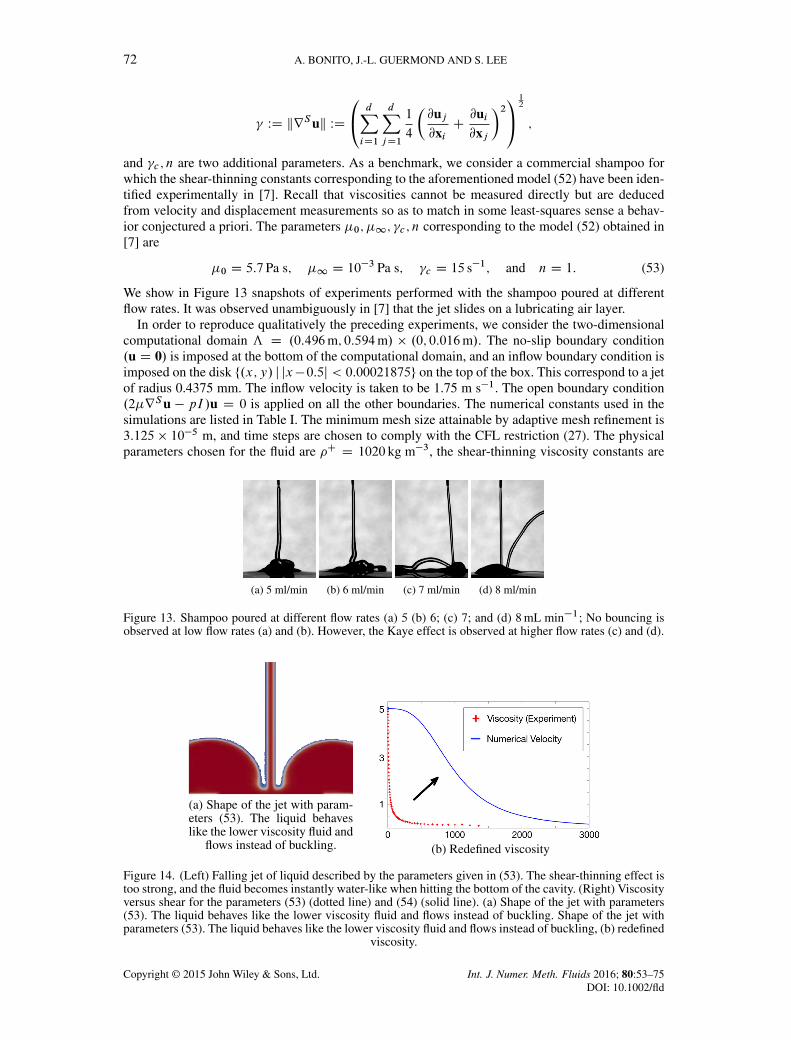
We show in Figure 13 snapshots of experiments performed with the shampoo poured at differentflow rates. It was observed unambiguously in [7] that the jet slides on a lubricating air layer.
In order to reproduce qualitatively the preceding experiments, we consider the two-dimensionalcomputational domain ƒ D .0:496m; 0:594m/ � .0; 0:016m/. The no-slip boundary condition.u D 0/ is imposed at the bottom of the computational domain, and an inflow boundary condition isimposed on the disk ¹.x; y/ j jx�0:5j < 0:00021875º on the top of the box. This correspond to a jetof radius 0.4375 mm. The inflow velocity is taken to be 1.75 m s�1. The open boundary condition.2�rSu � pI/u D 0 is applied on all the other boundaries. The numerical constants used in thesimulations are listed in Table I. The minimum mesh size attainable by adaptive mesh refinement is3:125 � 10�5 m, and time steps are chosen to comply with the CFL restriction (27). The physicalparameters chosen for the fluid are �C D 1020 kg m�3, the shear-thinning viscosity constants are
Figure 13. Shampoo poured at different flow rates (a) 5 (b) 6; (c) 7; and (d) 8mL min�1; No bouncing isobserved at low flow rates (a) and (b). However, the Kaye effect is observed at higher flow rates (c) and (d).
Figure 14. (Left) Falling jet of liquid described by the parameters given in (53). The shear-thinning effect istoo strong, and the fluid becomes instantly water-like when hitting the bottom of the cavity. (Right) Viscosityversus shear for the parameters (53) (dotted line) and (54) (solid line). (a) Shape of the jet with parameters(53). The liquid behaves like the lower viscosity fluid and flows instead of buckling. Shape of the jet withparameters (53). The liquid behaves like the lower viscosity fluid and flows instead of buckling, (b) redefined
Figure 15. (Left to Right, Top to Bottom) Numerical simulation of the Kaye effect with adaptive meshes(from left to right and top to bottom). The viscosity parameters are given in (54). The first and last framesillustrate the adaptive subdivision generated by the adaptive strategy. An air layer appears in the last framein the first row and is fully developed in the first frame of the second row. The apparition of the air layer
coincides with the beginning of the bouncing phenomenon.
provided in (54). We take �� D 1:2 kg m�3 and �� D 2 � 10�5 Pa s�5 for the air. Surface tensionis applied at the fluid/air interface with the surface tension coefficient � D 0:03N m�1.
After many numerical experiments, it turned out that the aforementioned physical parameters didnot give any Kaye effect. Our interpretation is that the shear-thinning effect given by the set ofparameters (53) is too strong; with these coefficients, the fluid instantly becomes water like whenhitting the bottom of the cavity (Figure 14(a)). Several explanations for this mismatch are plausible:(i) as mentioned earlier, the parameters (53) are measured under the assumption that the shear-thinning law follows the Cross model; (ii) the shear is over-predicted by our algorithm; (iii) theair layer width for this range of parameters is too thin to be captured by the algorithm; and (iv) afundamental component is missing in our mathematical model. These observations have lead us toconsider a different set of shear-thinning parameters requiring a larger shear for a notable reductionof the viscosity and a smoother transition from the maximum to the minimum values of the viscosity(Figure 14(b)). The parameters that we now consider are the following:
�0 D 5:7Pa s�3; �1 D 10�3 Pa s; �c D 970 s�1 and n D 3: (54)
This set of parameter produces the Kaye effect as shown in Figure 15. Here again, we notice thatthere is a very thin layer of air between the bouncing jet and the rest of the fluid, thereby adding tothe large body of evidence pointing at the importance of air layers in bouncing jets. Let us finallymention that these computations show also that mesh adaptivity is critical to reproduce numericallythe Kaye effect.
6. CONCLUSION
Newtonian and non-Newtonian (Kaye effect) bouncing jets have been successfully reproducednumerically. A level set representation has been employed to track the interface between two immis-cible incompressible fluids modeled by the incompressible Navier–Stokes equations with variabledensity and viscosity.
In agreement with experimental results, we have found that the creation of a thin lubricat-ing layer of air between the jet and the rest of the fluid is a critical aspect of this phenomenon.Capturing numerically such a thin layer was possible upon designing algorithms capable of effi-ciently reproducing the evolution of a level set function with a sharp transition layer. Among the
numerical tools that helped us achieve this goal are (i) a reinitialization algorithm based on a hyper-bolic tangent filter; (ii) an (on the fly) entropy viscosity stabilization technique coupled with anexplicit SSP Runge–Kutta 3 discretizations in time; and (iii) an adaptive finite element methodtailored to interface problems described by level set functions. Several two-dimensional and three-dimensional numerical benchmark problems have been provided to validate our method and therebygave credibility to our findings.
ACKNOWLEDGEMENTS
The experiments reported in the paper were carried out at the High Speed Fluid Imaging Laboratory ofS. Thoroddsen at KAUST during two visits of S. L. The authors would like to express their gratitude toS. Thoroddsen and E. Li for their help in conducting these experiments. W. Bangerth availability and hisconstant help in the implementation of our algorithms with the deal.II library is acknowledged. The authorsacknowledge the Texas A&M University Brazos HPC cluster that contributed to the research reported here.
This work has been supported by the National Science Foundation through grant DMS-1254618 and theKing Abdullah University of Science and Technology award KUS-C1-016-04.
REFERENCES
1. Thrasher M, Jung S, Pang YK, Chuu CP, Swinney HL. Bouncing jet: a Newtonian liquid rebounding off a freesurface. Physical Review E 2007; 76:056319.
2. Lockhart T. Bouncing of Newtonian liquid jets, 2014. (Available from: https://www.uwec.edu/Physics/research/lockhartjets.htm) [Accessed on 30 January 2013].
3. Kaye A. A bouncing liquid stream. Nature 1963; 197:1001.4. Collyer A, Fischer PJ. The Kaye effect revisited. Nature 1976; 261:682.5. Versluis M, Blom C, van der Meer D, van der Weele K, Lohse D. Leaping shampoo and the stable Kaye effect.
Journal of Statistical Mechanics: Theory and Experiment 2006; 2006(07):P07007.6. Binder JM, Landig AJ. The Kaye effect. European Journal of Physics 2009; 30(6):S115.7. Lee S, Li EQ, Marston JO, Bonito A, Thoroddsen ST. Leaping shampoo glides on a lubricating air layer. Physical
Review E 2013; 87:061001.8. Ochoa J, Guerra C, Stern C. New experiments on the Kaye effect. In Experimental and Theoretical Advances in Fluid
Dynamics, Environmental Science and Engineering, Klapp J, Cros A, Velasco Fuentes O, Stern C, Rodriguez MezaMA (eds). Springer: Berlin Heidelberg, 2012; 419–427.
9. Cross MM. Rheology of non-Newtonian fluids: a new flow equation for pseudoplastic systems. Journal of ColloidScience 1965; 20(5):417–437.
10. Chorin AJ. Numerical solution of the Navier–Stokes equations. Mathematics of Computation 1968; 22:745–762.11. Témam R. Sur l’approximation de la solution des équations de Navier–Stokes par la méthode des pas fractionnaires.
II. Archive for Rational Mechanics and Analysis 1969; 33:377–385.12. Osher S, Sethian JA. Fronts propagating with curvature-dependent speed: algorithms based on Hamilton–Jacobi
formulations. Journal of Computational Physics 1988; 79(1):12–49.13. Bonito A, Guermond JL, Popov B. Stability analysis of explicit entropy viscosity methods for non-linear scalar
conservation equations. Mathematics of Computation 2014; 83(287):1039–1062.14. Ville L, Silva L, Coupez T. Convected level set method for the numerical simulation of fluid buckling. International
Journal for Numerical Methods in Fluids 2011; 66(3):324–344.15. Guermond JL, Pasquetti R, Popov B. Entropy viscosity method for nonlinear conservation laws. Journal of
Computational Physics 2011; 230(11):4248–4267.16. Gottlieb S, Shu CW, Tadmor E. Strong stability-preserving high-order time discretization methods. SIAM Review
2001; 43(1):89–112.17. Shu CW, Osher S. Efficient implementation of essentially non-oscillatory shock-capturing schemes. Journal of
Computational Physics 1988; 77(2):439–471.18. Guermond JL, Shen J. On the error estimates for the rotational pressure-correction projection methods. Mathematics
of Computation 2004; 73(248):1719–1737 (electronic).19. Guermond JL, Minev P, Shen J. Error analysis of pressure-correction schemes for the time-dependent Stokes
equations with open boundary conditions. SIAM Journal on Numerical Analysis 2005; 43(1):239–258 (electronic).20. Guermond JL, Salgado A. A splitting method for incompressible flows with variable density based on a pressure
Poisson equation. Journal of Computational Physics 2009; 228(8):2834–2846.21. Bonito A, Guermond JL, Lee S. Modified pressure-correction projection methods: Open boundary and variable
time stepping. In Numerical Mathematics and Advanced Applications - ENUMATH 2013, vol. 103, Lecture Notes inComputational Science and Engineering, 2015; 623–631.
22. Bänsch E. Finite element discretization of the Navier–Stokes equations with a free capillary surface. NumerischeMathematik 2001; 88(2):203–235.
23. Hysing S, Turek S, Kuzmin D, Parolini N, Burman E, Ganesan S, Tobiska L. Quantitative benchmark computa-tions of two-dimensional bubble dynamics. International Journal for Numerical Methods in Fluids 2009; 60(11):1259–1288.
24. Dziuk G, Elliott CM. An Eulerian approach to transport and diffusion on evolving implicit surfaces. Computer andVisualization in Science 2010; 13(1):17–28.
25. Gilbarg D, Trudinger NS. Elliptic Partial Differential Equations of Second Order, Classics in Mathematics. Springer-Verlag: Berlin, 2001. Reprint of the 1998 edition.
26. Engquist B, Tornberg AK, Tsai R. Discretization of Dirac delta functions in level set methods. Journal ofComputational Physics 2005; 207(1):28–51.
27. Tornberg AK. Interface tracking methods with application to multiphase flows, Royal Institute of Technology,Doctoral Dissertation, 2000.
28. Bonito A, Nochetto RH. Quasi-optimal convergence rate of an adaptive discontinuous Galerkin method. SIAMJournal on Numerical Analysis 2010; 48(2):734–771.
29. Bangerth W, Hartmann R, Kanschat G. deal.II — a general purpose object oriented finite element library. ACMTransactions on Mathematical Software 2007; 33(4):24/1–24/27.
30. Bangerth W, Heister T, Heltai L, Kanschat G, Kronbichler M, Maier M, Turcksin B, Young TD. The deal.iilibrary, version 8.1. arXiv preprint, 2013.
31. Gabriel E, Fagg G. E, Bosilca G, Angskun T, Dongarra JJ, Squyres JM, Sahay V, Kambadur P, Barrett B, LumsdaineA, Castain RH, Daniel DJ, Graham RL, Woodall TS. Open MPI: goals, concept, and design of a next generation MPIimplementation. Proceedings, 11th European PVM/MPI Users’ Group Meeting, Budapest, Hungary, 2004; 97–104.
32. Burstedde C, Wilcox LC, Ghattas O. p4est: scalable algorithms for parallel adaptive mesh refinement on forests ofoctrees. SIAM Journal on Scientific Computing 2011; 33(3):1103–1133.
33. Zalesak ST. Fully multidimensional flux-corrected transport algorithms for fluids. Journal of Computational Physics1979; 31(3):335–362.
34. Rising bubble benchmark problems, 2014. (Available from: http://www.featflow.de/en/benchmarks/cfdbenchmarking/bubble.html) [Accessed on January 2015].
35. Bonito A, Picasso M, Laso M. Numerical simulation of 3D viscoelastic flows with free surfaces. Journal ofComputational Physics 2006; 215(2):691–716.
36. Tome M, McKee S. Numerical simulation of viscous flow: buckling of planar jets. International Journal forNumerical Methods in Fluids 1999; 29(6):705–718.