By Theodore Katsanis
Abstract. A finite-difference method for the solution of symmetric positive linear
differential equations is developed. The method is applicable to any region with
piecevvise smooth boundaries. Methods for solution of the finite-difference equa-
tions are discussed. The finite-difference solutions are shown to converge at es-
sentially the rate 0(h1'2) as h —> 0, h being the maximum distance between adjacent
mesh-points.
An alternate finite-difference method is given with the advantage that the
finite-difference equations can be solved iteratively. However, there are strong
limitations on the mesh arrangements which can be used with this method.
Introduction. In the theory of partial differential equations there is a funda-
mental distinction between those of elliptic, hyperbolic and parabolic type. Gen-
erally each type of equation has different requirements as to the boundary or
initial data which must be specified to assure existence and uniqueness of solutions,
and to be well posed. These requirements are usually well known for an equation
of any particular type. Further, many analytical and numerical techniques have
been developed for solving the various types of partial differential equations, sub-
ject to the proper boundary conditions, including even many nonlinear cases.
However, for equations of mixed type much less is known, and it is usually diffi-
cult to know even what the proper boundary conditions are.
As a step toward overcoming this problem Friedrichs [1] has developed a the-
ory of symmetric positive linear differential equations independent of type. Chu
[2] has shown that this theory can be used to derive finite-difference solutions in
two-dimensions for rectangular regions, or more generally, by means of a trans-
formation, for regions with four corners joined by smooth curves. In this paper a
more general finite-difference method for the solution of symmetric positive equa-
tions is presented (based on [3]). The only restriction on the shape of the region is
that the boundary be piecewise smooth. It is proven that the finite-difference solu-
tion converges to the solution of the differential equation at essentially the rate
0(h112) as h —> 0, h being the maximum distance between adjacent mesh-points
for a two-dimensional region. Also weak convergence to weak solutions is shown.
An alternate finite-difference method is given for the two-dimensional case with
the advantage that the finite-difference equation can be solved iteratively. How-
ever, there are strong limitations on the mesh arrangements which can be used
with this method.
1. Symmetric Positive Linear Differential Equations. Let Q be a bounded open
set in the m-dimensional space of real numbers, Rm. The boundary of Q will be
Received May 18, 1967. Revised May 8, 1968.
763
764 THEODORE KATSANIS
denoted by dQ, and its closure by Ö. It is assumed that du is piecewise smooth. A
point in Rm is denoted by x = (x\, xi, • • •, xm) and an r-dimensional vector-valued
function defined on Í2 is given by u = (u\, «2, • • -, ur). Also let a1, a2, -, am
and G be given r X r matrix-valued functions and / = (/i, /2, • • •, fr) a given r-
dimensional vector-valued function, all defined on Ü (at least). It is assumed that
the a* are piecewise differentiable. For convenience, let a = (a1, a2, • • -, am), so
that we can use expressions such as
(1.1) V.(«u)= Z¿-(«'«)•
m « m t. i m ~
V f * \ _ 'S-* i T"1 * i=i ó\C¿ î=i OX i i=\ ox i
simply as
The definitions for symmetric positive operators and admissible or semiad-
missible boundary conditions were introduced by Friedrichs [1].
Let K be the first-order linear partial differential operator defined by
(1.3) Ku = a -Vu + V- (aw) + Gu .
K is symmetric positive if each component, a\ of a is symmetric and the symmetric
part, (G + G*)/2, of G is positive definite on Ö.
For the purpose of giving suitable boundary conditions, a matrix, ß, is defined
(a.e.) on du by
(1.4) ß = n-a,
where n = (nh n2, • • -, nm) is defined to be the outer normal on d£2.
The boundary condition Mu = 0 on dfi is semiadmissible if M = ß — ß, where
ß is any matrix with nonnegative definite symmetric part, (ß + ß*)/2. If in addi-
tion, 3l(/¿ — |3) © 9I(m + ß) = Rr on the boundary, du, the boundary condition
is termed admissible. (3l(^ — ß) is the null space of the matrix (ß — ß).)
The problem is to find a function u which satisfies
/X 5) Ku = f on Í2,
Mm = 0 on du ,
where K is symmetric positive.
Many of the usual partial differential equations may be expressed in this sym-
metric positive form, with the standard boundary conditions also expressed as an
admissible boundary condition. This includes equations of both hyperbolic and
elliptic type. However, the greatest interest lies in the fact that the definitions are
completely independent of type. An example of potentially great practical im-
portance is the Tricomi equation which arises from the equations for transonic
fluid flow. The Tricomi equation is of mixed type, i.e., it is hyperbolic in part of
the region, elliptic in part, and is parabolic along the line between the two parts.
The significance of the semiadmissible boundary condition is that this insures
License or copyright restrictions may apply to redistribution; see https://www.ams.org/journal-terms-of-use
SYMMETRIC POSITIVE DIFFERENTIAL EQUATIONS 765
the uniqueness of a classical solution to a symmetric positive equation. On the
other hand, the stronger, admissible boundary condition is required for existence.
The existence of a classical solution is generally difficult to prove for any particular
case, and depends on properties at corners of the region.
Let 3C be the Hilbert space of all square integrable r-dimensional vector-valued
functions defined on 0. The inner product is given by
(1.6) (u, v) = j u-v ,
where
r
A boundary inner product is defined by
(1.8) (u,v)B = u-v > da
with the corresponding norm
The adjoint operators K* and M* are defined by
(1.10) K*u = -a-Vu - V-(au) + G*u ,
(1.11) M*u = (ß* + ß)u.
We will make use of the following lemmas by Friedrichs.
Lemma 1.1 (First Identity). If K is symmetric positive, then
(1.12) (v, Ku) + (v, Mu)B = (K*v, u) + (M*v, u)B .
Lemma 1.2 (Second Identity). If K is symmetric positive, then
(1.13) (u, Ku) + (u, Mu)b = (u, Gu) + (u, ßu)ß
Lemma 1.3. Suppose u is a solution to (1.5) where M is semiadmissible. Let XG be
the smallest eigenvalue of (G + G*)/2 in Ü. Then
(1.14) ||u|| ^ (1/XG)||/|| .
Lemma 1.4. Let u satisfy Eq. (1.5) where M is semiadmissible. Further, assume
that (ß + ß*)/2 is positive definite on du with smallest eigenvalue X,,. Then
(1.15) \\u\\b£ (1/(XGX,)1'2) 11/11
Lemma 1.3 insures the uniqueness of a classical solution, and also that it is
well posed in L2 for homogeneous boundary conditions.
By widening the class of solutions to (1.5) to include weak solutions it is quite
easy to prove existence of a solution to a symmetric positive equation under only
semiadmissible boundary conditions. We will use Friedrichs' definition of weak
License or copyright restrictions may apply to redistribution; see https://www.ams.org/journal-terms-of-use
766 THEODORE KATSANIS
solution. Let V = C\(ü) Pl {v\M*v = 0 on du}. A function u G 3C (defined
above) is a weak solution of (1.5) if / G 3C and for all v G U
(1.16) (v,f) = (K*v,u).
It follows from the "first identity" (1.12) that a classical solution is also a weak
solution.
Friedrichs [1] proved the existence of weak solutions if M is semiadmissible. He
also showed that, if, in addition, M is admissible and the weak solution is con-
tinuously differentiable, then the weak solution must also be a classical solution.
2. Finite-Difference Solution of Symmetric Positive Differential Equations. First
we will express K in a form slightly different from (1.3), by the use of (1.2). We
have
(2.1) Ku = 2V-(au) - (V-a)u + Gu .
Using the concept of vectors whose components are themselves matrices or
vectors leads to somewhat simpler notation for the application of Green's theorem.
Lemma 2.1 (Green's Theorem). Let g be a continuously differentiable m-
dimensional vector-valued function defined on ü C Rm, with vector components in
either R, RT or RT X RT. Then
(2.2) / V-g = j g-n. J a J ao
This result follows directly from the definitions, using Green's theorem.
We now integrate the equation Ku = / over any region PCS using (2.1)
and Green's theorem to obtain
(2.3) / Ku = 2 i ßu- i (V-a)w + [ Gu= ( f. j p j 3p j p j p j p
By a suitable approximation to (2.3) the desired finite-difference equations will be
obtained.
Let H be a set of N mesh-points for fi. It is not required for the theory that the
mesh-points all lie in Ü. With each mesh-point x¡ G H we identify a mesh-region
Pj C 0 by
Pj = {x\\x — Xj\ < \x — xk\, \/xk G H,k ?¿ j;x G Œ} .
If Pj is adjacent to Pk we say that x¡ is connected to Xk (corresponding to the fact
that the directed graph of the resulting matrix will have a directed path in both
directions between j and k, see [4, p. 16]). Let ljfk = \x¡ — Xk\, where Xj is connected
to Xk, and let h = max Ijj,. Now define A¡ to be the "volume" of Pj and L/,* to
be the "area" of the (r — 1)-dimensional "surface" between P¡ and Pk. We put
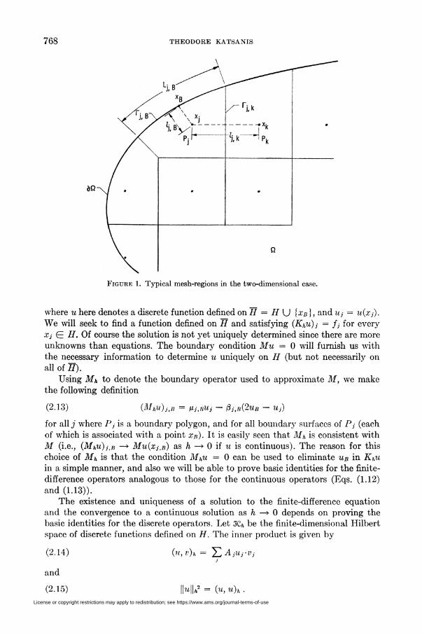
Tj,k = Pj H Pk- Fig. 1 illustrates mesh-points and corresponding mesh-regions
for two dimensions. This concept of mesh-regions is based on the suggestions of
MacNeal [5]. We will always use the notation ^, to indicate a sum over all points,
Xj, in H, and ^* to indicate a sum over points, xk, which are connected to some
one point, x¡.
SYMMETRIC POSITIVE DIFFERENTIAL EQUATIONS 767
The desired finite-difference equation can now be obtained by a suitable ap-
proximation to Eq. (2.3). We use the symbol = to indicate the discrete approxima-
tion that will be used for each expression. First
f o.. _!_ r a Ui + Uk(2.4) J ßu = Lj,kßj,k 2
where u¡ = u(x¡) and ßj,k is the value of ß for P¡ at the center of T¡,k. (Note that
ßjtk = —ßk.j.) The approximation to the next term of Eq. (2.3) requires approxi-
mating u with Uj first, and then applying Green's theorem before approximating a.
With this we obtain
(2.5) / (V-a)u= (V-a)Uj= ßuj. J Pj J Pj J BPj
The final approximation is then
(2.6) / ßuj = Lj,kßj,kUj. Ti.k
Equations (2.4) and (2.6) take care of the integration over the interface between
any Pj and Pk. Now we need to make an approximation for the boundary sides.
It will be convenient to be able to subdivide Pj D du into more than one piece.
We will label each piece Tj,b and we will use the convention that ^2b will mean a
summation over the B for just one j. We use Ij,b to denote the distance from x¡
to xb, where xb is located at the "center" of Tj¡B and Lj,B is used for the "area"
of Tj,B- Also ßj,s = ß(xß). This notation is indicated for the two-dimensional case
in Fig. 1. The desired approximations are now given by
(2.7) J ßu = Lj,Bßj,BUB, Ti.B
(2.8) / ßuj = Lj,Bßj,BUj.
Finally the remaining terms in equation (2.3) are approximated by
(2.9) I Gu = AjGjUj, J Pi
(2.10) / f^Ajfj,J Pi
where Gj = G(x¡) and/,- = f(x¡). Also we can approximate ¡Ku by
(2.11) / Ku = Aj(Khu)j, J pj
where Kh is the finite-difference operator to be defined and which will approximate
K. Using approximations (2.4) to (2.11) in Eq. (2.3) we arrive at the following
definition of Kh,
License or copyright restrictions may apply to redistribution; see https://www.ams.org/journal-terms-of-use
768 THEODORE KATSANIS
Figure 1. Typical mesh-regions in the two-dimensional case.
where u here denotes a discrete function defined on H = H U \xB}, and u¡ = u(x¡).
We will seek to find a function defined on H and satisfying (Khu)¡ = /y for every
Xj G H- Of course the solution is not yet uniquely determined since there are more
unknowns than equations. The boundary condition Mu = 0 will furnish us with
the necessary information to determine u uniquely on H (but not necessarily on
all of H).
Using Mh to denote the boundary operator used to approximate M, we make
the following definition
(2.13) (Mhu)j,B = ßj,BUj - ßj,B(2uB - Uj)
for all j where Pj is a boundary polygon, and for all boundary surfaces of Pj (each
of which is associated with a point xB). It is easily seen that Mh is consistent with
M (i.e., (Mhu)j,B -* Mu(xj,B) as h —> 0 if u is continuous). The reason for this
choice of Mh is that the condition Mhu = 0 can be used to eliminate uB in Khu
in a simple manner, and also we will be able to prove basic identities for the finite-
difference operators analogous to those for the continuous operators (Eqs. (1.12)
and (1.13)).
The existence and uniqueness of a solution to the finite-difference equation
and the convergence to a continuous solution as h —* 0 depends on proving the
basic identities for the discrete operators. Let 5Ch be the finite-dimensional Hubert
space of discrete functions defined on H. The inner product is given by
(2.14) (u, v)k = J^AjUj-Vj j
and
License or copyright restrictions may apply to redistribution; see https://www.ams.org/journal-terms-of-use
SYMMETRIC POSITIVE DIFFERENTIAL EQUATIONS 769
Also a "boundary" inner product is given by
(2.16) (u,v)Bh=J2 X Lj,llUj,B-Vj,B j B
for Pj a boundary mesh region, and
(2.17) \\u\\2Bh=(u,u)Bh.
The discrete adjoint operators K* and Mh* are defined in the obvious way,
(2.18) Aj(Kh*u)j = - X Lj,kßj,kUk - X Lj,Bßj,B(2uB - My) + Aßj*Uj, k U
(2.19) (Mh*u)j,B = U*j,BUj + ßj,B(2uB - My) .
We can now give the "first identity" for the discrete operators.
Lemma 2.2. If K is symmetric positive, then
(2.20) (v, Khu)n + (v, Mhu)Bh = (Kh*v, u)h + (Mh*v, u)Bh
for any functions u, v defined on H.
Proof. Using the definitions, Eqs. (2.12) and (2.18), we have
(v,Khu)h — (Kh*v,u)h = X IL Lj,kVj-ßj,kuk y L k
+ HLj,BVj-ßj,B(2uB — My) + Aji'j-GjUj u
+ £ Lj,Bßj,B(2vB — Vj)-Uj — AjGj*Vj-Uj . B -I
By rearrangement, since ßj,k = —ßk,j, and since ßj,k is symmetric we have
S X) Lj,kßj,kVk-Uj = — X X Lj.kVj-ßj,kUk j k y à-
and we see that all terms cancel with the exception of the boundary terms, so that
(v,Khu)h — (Kh*v, u)h
j H
On the other hand, using Eqs. (2.13) and (2.19),
(Mk*v, u)B. - (v, Mhu)Bh = X H LjtB(ßXßVj-Uj + ßj,B(2vB — v,)-u¡) ] B
- J2 ÜLj.B&j-ßj.BUj - Vj-ßj,B(2uB - My)) j B
which is the same as the right side of (2.21). Hence the "first identity" for the dif-
ference operators is proved.
The discrete operators have been defined so that Kh + Kh* = G + G* and
Mh + Mh* = ß + m*. By letting v = u in (2.20) we can prove the discrete "second
identity" as for the continuous case.
Lemma 2.3. // K is symmetric positive, then
(2.22) (u, Khu)h + (u, Mhu)Bh = (u, Gu)h + (u, ßu)Bh.
License or copyright restrictions may apply to redistribution; see https://www.ams.org/journal-terms-of-use
770 THEODORE KATSANIS
Using Eq. (2.13) and Mhu = 0 we can eliminate ub from Eq. (2.12) so that
the equation Khu = f can be reduced to
(2.23) X Lj,kßj,kUk + X Lj,Bßj,BUj + AjGjUj = Ajf¡, Vj . k B
If we consider the case when Í2 is two dimensional and rectangular, and the Pj are
all equal rectangles, we can compare (2.23) with the finite-difference equation ob-
tained by Chu [2]. The equation obtained by Chu is the same as (2.23) for interior
rectangles, but is different for boundary rectangles.
Let A be the rN X rN matrix of coefficients of (2.23). Letting (u, v) = X/j ui'vi>
the ordinary vector inner product, we have
(2.24) (u, Au) = (m, Khu)h + (u, Mhu)Bh.
Hence, by the "second identity" (2.22), A has positive definite symmetric part
which shows that A is nonsingular. We can also obtain an a priori bound forj|M||A
just as in the continuous case.
Lemma 2.4. Suppose u is a solution to KhU = /, Mhu = 0, where K is symmetric
positive and M is semiadmissible. Then
(2.25) ||«|U á (lAo)ll/ll» •
// in addition, (ß + ß*) is positive definite on dfi, then
(2-26) \\u\\bk á Q¿y7"211/11* .
These bounds are obtained from the "second identity."
It is possible to show that the solution of the finite-difference equation (2.23)
converges strongly to a continuously differentiable solution of equation (1.5), under
the proper hypotheses. For simplicity we prove convergence only for the case when
Í2 is two dimensional (m = 2). Extension to regions in higher dimensions, with the
same rate of convergence, follows directly. To allow the type of comparison we
wish to make we will define operators mapping 5C into Kh and vice versa. Let
rh: K —> Kh be the projection defined by
(2.27) (rhu)j = u(xj) for all x¡ G H .
In the other direction, let ph: Kh —» K be an injection mapping defined by
(2.28) PhUh(x) = (uh)j, for all x G Pj -
We immediately have the following relations,
(2.29) nph = / ,
(2.30) |b,M„|| = ||m*||„ for all uh G 3d .
We can now state our basic convergence theorem for two-dimensional regions.
Theorem 2.1. Suppose that u G C2(S2) satisfies
Ku = / on ü C Ä2,
Mu = 0 on dQ,,
where K is symmetric positive, and ß + ß* is positive definite on du. For any given
License or copyright restrictions may apply to redistribution; see https://www.ams.org/journal-terms-of-use
SYMMETRIC POSITIVE DIFFERENTIAL EQUATIONS 771
h > 0, let Hh be a set of associated mesh-points such that the maximum distance between
connected nodes is less than h and also that Lj,k, Lj.b and \x — x¡\ for x G P¡ are all
less than h. It is assumed that the mesh is sufficiently regular so that h2/A y for each Pj
is bounded independently of h by a constant Ki > 0, which is possible for sufficiently
nice regions. Also it is assumed that a uniform rectangular mesh is used for all Pj any
point of which is at a dislance greater than Kihfrom dû, where Ki is a positive constant.
It is assumed that a G C2(Ü).
Let Uh G 3C>, be the unique solution to
Khuh = rhf on Hh , Mhuh = 0 .
Then \\phuh — u\\ = 0(h") ash —> 0/or any positive v < 1/2.
Chu [2] proved convergence of his finite-difference scheme, where Q is a rectangle
or a region with four corners, but the rate of convergence was not established.
Proof. Define wh = uh — rhu. Let X<j be the smallest eigenvalue of (G + G*)/2
in Ü. Using the "second identity" (2.22), we have
\\wh\\h2 á (1/Xg)[(m>a, KhWh)h + (wh, Mhwh)Bh]
Using the Cauchy-Schwartz inequality, we have
(2.31) IKIU2 ^ (l/\a)(\\wh\\h\\KhWh\\h + \\wh\\Bh\\MhWh\\Bh) .
We will show that \\Khwh\\h = 0(hV2) and \\MhWh\\Bh = 0(h), as h -> 0. We shall
need the following lemma.
Lemma 2.5. Let g be a function defined on a finite region P C R2, and suppose
that g satisfies a Lipschitz condition, i.e., there is a constant K¡ > 0 such that
\d(x) ~ $(y)\ = Kz\x — y\, for all x, y G P. Then, if A<> is the area of P and
\x — xq\ g h in P,
aJ,g(x0) - ~r I g(x)\ g Kih.
We proceed now with the proof of the theorem. Let Í2i denote that portion of
ß consisting of those Pj which are rectangular, and let 02 denote the rest of the P¡.
From the hypothesis we see that the area of 02 is less than the length of 30 times
Kih. We have now that
(2.32) ||K»w»||i = L / (Ku(xj)- (Khrhu)j)2+ E / (Ku(x,) - (Khrhu)j)2, jSjt •> Pj jGjt J Pi
where
J<= {¿IP/CO,}, ¿-1,2.
To simplify notation we will use Wy for u(x¡) and uB for u(xB). We now obtain a
suitable bound for \Ku(xf) — (Kh.rh.u)j\
\Ku(xj) — (Khrhu)j\
Consider the first term in the last expression above
2V- (au) (xj) - ¿Z^ßjAuj + uk) - 2 T.^PùbUb k Aj b Aj
+ (V-a)u(xj) - Yi,~t^ßi,kUj - X)- k Aj b Aj
License or copyright restrictions may apply to redistribution; see https://www.ams.org/journal-terms-of-use
772 THEODORE KATSANIS
2V- (aw) (Xj) - £ ^ /3y,4(My + Uk) - 2 £ ^ ft,!,«* t ^-3 IS Aj I
2V-(aM)(zy) / V-(cm)
+ T X / ßj,k(2uj,k - (uj + uk)) Aj\ k JTjik
By Lemma 2.5, since a and u G C2(fi) imply that their derivatives satisfy a Lip-
schitz condition,
(2.35) = 0(h) .2V-(«u)(xj)--~j V-(au) i Pj I
We consider now the case when j G J\, so that P¡ is a rectangle with Xj at
the center.
7 72 My = My.fc - "y My,* + J^ u' (£1) ,
7 V fc_ „,//
«"(«•) , 2 "'• ' (4)2
where the derivatives are directional derivatives in the direction xk — x¡. Hence,
if |m"| < Kz in 0, we have
\2Uj,k- (Uj + Uk)\ < (K3/i)h2
This means that
(2.36) / ßj.k(2Uj,k - (My + uk)) Ú Lj,k\\ßj,k\\ \2uj,k - (uj + uk)\= 0(h3)
when j G Ji.
We now examine a Taylor series expansion for /3m about the point xjik =
(xj + xk)/2.
ß(Xj,k — tz)u(xj,k — tz) = (ßu)jik — t
where 2 is a unit vector orthogonal to Xj — xk, t is a scalar parameter, g(%) =
(gÁ£i), gÁíi), • • •> gAZr)), gi is the ¿th component of the vector (d2/dt2)(ßu), and £t
is a point on the straight line between xjik + (Ljtk/2)z and x¡,k — (L¡,k/2)z. Using
(2.37) we obtain the following bound,
License or copyright restrictions may apply to redistribution; see https://www.ams.org/journal-terms-of-use
SYMMETRIC POSITIVE DIFFERENTIAL EQUATIONS 773
(2.38) f
Now, using (2.35), (2.36) and (2.38) in (2.34) we obtain
2V- (au) (xj) — £ ~jr ßj.k(uj + Uk)(2.39) Aj = 0(h)
for all j G Ji, since h2/A¡ ^ Ki and the boundary terms are not present.
Consider now the second term on the right of (2.33) :
(V-a)u(xj) v"* Lj,k
+ AylV-'ry,, 08 - ßilk)uj + S/ 03 - /33.,s)My
By Lemma 2.5
(2.41) (V-a)u(xj) -~ (V-a)w = 0(A) . Ay
Next, since u satisfies a Lipschitz condition, \x — xy| < /i for all x G •?>•> and
since 11V-a 11 is uniformly bounded in 0, we have
(2.42) dipAj (V-a)(u — Uj) = 0(h) .
Finally, since ßjik and ßj,B are each evaluated at the midpoint of Ty^ or Ty.ß,
respectively, we can use a Taylor series analysis, as in deriving equation (2.38),
to obtain
(2.43) Aj X / 03 - ßj.k)uj + Z / 08 - ßj,B)uj * r;,fc B ri.B
Combining (2.41), (2.42), and (2.43) in (2.40) we obtain
'a)u(Xj) - E^
(2.44) Aj ßj.kUj ZLj,B 0 0(h)
Note that (2.44) holds for all j, not just îorj G Ji-
We can now substitute (2.39) and (2.44) in (2.33) to obtain
(2.45) \Ku(xj) — (Khrhu)j\ = 0(h) for all/ G </i.
We cannot obtain as good a bound for \Ku(xj) — (Khrhu)j\ when j G Ji,
although (2.44) holds, since Tj,k is not in general bisected by the line between x¡
and xk. However, we can show that \Ku(x¡) — (Khrhu)j\ is uniformly bounded for
j G Ji, which is adequate since the area of O2 is of order h. The two inequalities
which must be re-examined are (2.36) and (2.38). We now have, since u and (/3m)
satisfy Lipschitz conditions, that
774 THEODORE KATSANIS
/ /3m - (ßu)j,H = O(A2) .
Using this, with the other results which still hold, we see that \Ku(x¡) — (Khrhu)j\
is uniformly bounded for j G Ji, as h —» 0. Using this, together with (2.45) in
(2.32) we obtain
(2.49) \\KhWh\\h = 0(h>12) .
The next step is to show that \\MhWh\\Bh = 0(h). We have
\\Mhwh\\B = \\Mhrhu\\Bll
since MhUh = 0. Now
However, using the fact that ßj,BUß = ßj.ßUß,
Ißj.BUj — ßj,ß(2uB — Uj)\ = 0(h)
since m is differentiable, and ||jli|| and ||/3|| are uniformly bounded. This shows
that
IIM^mHb, = 0(h2) ,
since £y,B Ljjs is simply the length of dû. This proves that
(2.50) \\MhWh\\Bh = 0(h) .
(2.51) |K||Ä2 = \\wh\\hO(híl2) + |K||bäO(ä) .
From Lemma 2.4, ||w>a||/sa must be bounded, since
IKIK S \\uh\\Bh+ \\rhu\\Bk
- ^ , si/ülK/llfr + lk*wlU4 (,X(jAM;
which is certainly uniformly bounded as h —> 0. Likewise \\wh\\h is bounded. So
from (2.51) we have
(2.52) |K||„ = 0(/V'<) .
However, if we use (2.52) in (2.51) we get ||io*||j> = 0(h3li), or by repeating this
procedure enough times,
SYMMETRIC POSITIVE DIFFERENTIAL EQUATIONS 775
(2.53) IW|a = 0(h") , for any positive v < 1/2 .
Finally, we establish the convergence rate for \\phuh — u\\. We have
(2.54) \\phUh — u\\ ^ \\wh\\h + \\phrhu — u\\ .
The last term can be estimated by
(2.55) \\phrhu - «||2 = Z / (My - m)2 = 0(h2) . i jpj
Using (2.53) and (2.55) in (2.54) we get
(2.56) \\phuh - «|| = 0(/V) + 0(h) = 0(h") , for any positive v < 1/2 .
This completes the proof of Theorem 2.1.
This finite-difference method can be applied to the Tricomi equation ([1], [3]).
It is worthwhile noting that the solution obtained by the finite-difference solution
of the symmetric positive form of the Tricomi equation consists of derivatives of
the stream function, which corresponds to velocities in the physical problem. Hence,
even though we have a convergence rate which is less than 0(h112), it is essentially
equivalent to a convergence rate of 0(h312) if the original second-order equation
were solved directly for the stream function.
If a rectangular mesh is used, we can partition the matrix A so as to be block
tridiagonal. The matrix equation can then be solved by the block tridiagonal algo-
rithm ([6] and [4, p. 196]). Schecter [6] shows that this algorithm is valid for any
matrix with definite symmetric part. We have already shown that A has positive
definite symmetric part. Schecter [6], also suggests an alternate procedure for re-
ducing the computer storage requirements in solving the matrix equation.
An alternate method of solution may be possible in some cases. A may be de-
composed as A = D + S where D is Hermitian and S is skew symmetric. If the
smallest eigenvalue, Xb, of D is larger than the spectral radius, p(S), of S, then
IID^aSU < 1. In this case we can use a simple iterative method. Let w(0) be arbitrary,
and define u(i) recursively by DuU) = — Suii~~1) + /. In this case lim,._w m(í) = u.
In general, though, the eigenvalues of D will not be sufficiently large for this simple
method to work. However, the original finite difference equations can be modified
in some cases by the addition of a "viscosity" term, so as to obtain a convergent
iterative procedure for the solution of the matrix equation. This will be discussed
further in the next section.
We can consider the discrete analogue of a weak solution. Let Vk be the set
of discrete functions, vh, defined on H and satisfying Mh*vh = 0. For a discrete
weak solution, uh, we would then require that
(2.57) (Kh*vh, uh)h = (vh, r,J)h for all v E Vh.
From the "first identity" (2.20) we have then
(2.58) (vh, rhf)h = (vh, Khuh)h + (vh, Mhuh)Bh for all »£7»,
We see from this that (KhUh)j = f j for all P¡ which are not on the boundary, by
choosing (vh)j = 1, and (vh)k = 0 for k ^ j. Because of the discrete nature of the
equations we are not assured of uk satisfying the boundary conditions. However,
License or copyright restrictions may apply to redistribution; see https://www.ams.org/journal-terms-of-use
776 THEODORE KATSANIS
conversely, if uh satisfies Khuh = Thf and Mhuh = 0 we see immediately that (2.57)
must be satisfied.
Chu [2] has shown weak convergence of his finite-difference solution to a weak
solution of a symmetric positive equation and Cea [7] has investigated generally
the question of weak or strong convergence of approximate solutions to weak solu-
tions of elliptic equations. Using these ideas, we can prove weak convergence of
our finite-difference solutions to weak solutions of symmetric positive equations.
Theorem 2.2. For any h > 0, let Hh be a set of mesh points satisfying the require-
ments of Theorem 2.1. It is assumed that a G C2(Ü). Let «a be the unique solution to
Khuh = rhf, MhUh = 0.
If {A¿}?=i is a positive sequence converging to zero, then {phiUhi}'i=i has a sub-
sequence which converges weakly in H to a weak solution, u, of Eq. (1.5), that is
(K*v, u) = (v, f) for all v e.V. Furthermore, if u is a unique weak solution, then {ph^hf} t=i converges weakly to u.
Proof. First we note that ||phuh\| is bounded, since ||phuh11 = ||wA||Ä (l/^G)\\nf\\h,
by Lemma 2.4. Hence, there is a subsequence of {phiUiH} that converges weakly to
some m G 3C. (See Theorem 4.41-B, Taylor [8].) For convenience of notation we will
suppress the subscripts on the h.
We have, for all v G V,
(2 59) ' (Kh*ThV> M*)* ~~ (K*v> T>hU^\
Ú (\\Kh*rhv - rhK*v\\h + \\phrhK*v - K*v\\)\\phuh\\ .
But \\phrhK*v — K*v\\ —> 0, and in Theorem 2.1 we can substitute K* for K in
equation (2.49) to show that \\Kh*rhv — rhK*v\\ —> 0 (since Khwh = rhKu — Khrhu).
Since IIpaMaH is bounded,
lim | (Kh*rhv, uh)h — (K*v, phuh) | = 0 . A-.0
However, since K*v G K, we know that limA^0 (K*v, phUlt) = (K*v, u).
We have shown, then, that
(2.60) lim (Kh*rhv, uh)h = (K*v, u) for all v G V .
The discrete "first identity," Eq. (2.20), gives
(2.61) (K,*rhv, uh)h + (M*rhv, uh)Bh = (rhv, r^f)h.
Hence
(2.62) \(Kh*rhv, uh)h - (rhv, r¡J)*| 11^*^11^1^11*,.
By Lemma 2.4 ||ma||ba á H^WHa/OVX,,)1'2 which is bounded. Also, the proof of
equation (2.50) shows that limÄ_0 ||M*rAw||B/i = 0, for all v G V, so that
(2.63) lim | (Kh*rhv, uh)h — (rhv, rhf)h\ = 0 . A->0
Further, it is obvious that
(2.64) lim (mi, rhf)h = (v, f) . A-.0
License or copyright restrictions may apply to redistribution; see https://www.ams.org/journal-terms-of-use
SYMMETRIC POSITIVE DIFFERENTIAL EQUATIONS 777
Combining (2.60), (2.63) and (2.64) gives
(K*v,u) = (v,f) for all y G V ,
which completes the proof of the theorem.
3. Special Finite-Difference Scheme for Iterative Solution of Matrix Equation.
As pointed out in Section 2, the matrix equation Au = / can be solved by an
iterative procedure if the eigenvalues of the diagonal coefficient matrix are suffi-
ciently large compared to the eigenvalues of the off-diagonal coefficient matrix.
Following the idea of Chu [2] we modify the finite-difference equation by adding
a "viscosity" term which will have a diminishing effect on the finite-difference
equations as h —» 0, and yet will assure the convergence of an iterative method.
Unfortunately, the method is not applicable to every arrangement of mesh-points.
In fact there are rather severe restrictions which must be met. The first require-
ment is that the difference in areas of adjacent mesh-regions be sufficiently small.
This cannot be readily done along an irregular boundary, however, unless the
boundary is modified. A problem arises if the boundary is modified. The boundary
condition is given by Mu = (ß — ß)u = 0 on dû. We need to extend M to be de-
fined in a neighborhood of the boundary. It is possible to extend M continuously
in a neighborhood of the boundary. However, if the direction of the boundary
changes, ß changes drastically, and we have no assurance that ß will be positive
definite. The second requirement then is that M can be extended continuously
over a neighborhood of the boundary, in such a way that ß will have positive
definite symmetric part along the approximating boundary.
Let uh be an approximation to û. ûh will have to meet several requirements to
be specified later. Hh will denote a set of mesh-points associated with ûh and with
maximum distance h between connected nodes, and Hh will denote Hh U {xB}.
The discrete inner product is given by
(3.1) (uh,Vh) = \y,Aj(uh)j-(vh)j i
with the Aj being the area of Pj C ûh. Similarly, the "boundary" inner product
is changed so that the lengths, Lj,B, are the lengths along dûh.
We define now two new finite-difference operators, Kh and Mh, by
(3.2) (K„u) j = (Khu) j + £ a ^=^ + X ° ^^ , k tj.k B lj,B
_ aA. (3.3) (Mhu)j,B = (Mhu)j,B - 7—r— («y - uB) ,
Lij,Blj,B
where a is a positive number which must satisfy requirements to be specified later.
It will be useful to prove a slightly different version of the "second identity."
Lemma 3.1. If K is symmetric positive, then
(3.4) (uh, Khuh)h + (uh, MhUh)Bh = (uh, Guh)h + (uh, ßUh) Bh + X 7~^ (ui — uk) a.k) tj,k
where Xo'.*) indicates a sum over every (j, k) pair where x¡ is connected to xk.
Proof. Using the "second identity" for Kh and Mh, Eq. (2.22), we have
License or copyright restrictions may apply to redistribution; see https://www.ams.org/journal-terms-of-use
778 THEODORE KATSANIS
+ 1 E f-* My (My — Uk) j k tj,k
+ E I 1-l Uj- (Uj — UB) ; B tj.B
- Z I I—l Uj- (Uj — UB) . j B tj,B
The last two terms cancel. For the other term we have
Z Z T1 Uj- (uj — Uk) = Z T^ (u> ~ Uk^ 3 k tj,k (j,k) tj.k
which completes the proof.
Lemma 3.1 immediately assures the existence and uniqueness of a solution for
the special finite-difference scheme. Using MhUh = 0 to eliminate uB from KhUh =
Thf, we obtain
•5) Z ( Li.kßi.k -~I)Uk + [AjGj+ 1^/+ Z Lj,Bßj,B Uj = Ajfj k \ tj,k / \ k tj.k B /
for all Xj G Hh.
Let A be the matrix of coefficients of (3.5).
Lemma 3.2. If K is symmetric positive, then Khuh = rhf, Mhuh = 0 has a unique
solution on Hh-
(m, Au) = (uh, Khuh)h + (uh, MhUh)Bh
By Lemma 3.1 A has positive definite symmetric part, and hence is nonsingular.
Thus (3.5) defines M;, uniquely on Hh.
Also it will be noted that the "second identity" of Lemma 3.1 will give the
same a priori bounds for ||wä||* and ||m*||bä as given by (2.25) and (2.26).
We will now show that the special finite-difference scheme converges to a smooth
solution, under a number of hypotheses given in the theorem. The theorem also
includes all the hypotheses needed to assure convergence of the iterative matrix
solution. Though quite a number of requirements are given, there are only two
essential restrictions, namely, that the areas Aj must be nearly uniform, and that
M can be specified on a modified boundary in such a way that ß remains positive
definite.
Theorem 3.1. Suppose that u G C2(û) satisfies Ku = / on Û, Mu = 0 on dû,
where K is symmetric positive. For any h > 0, let ûh be an approximation to Û, and
let Hh be a corresponding set of mesh points with maximum distance h between con-
nected nodes, and also with Lj,k, L¡,b, and \x — Xj\ for x G Pj all less than h. It is
assumed that the following hypotheses are satisfied:
(i) There exists Ki > 0, independent ofh, such that for every P ¡we have h2/A¡ < K\.
(ii) There exists Ki > 0, independent of h, such that all Pj with any point at a
distance greater than Kih from dû are equal rectangles.
(iii) There exists K% > 0, independent of h, such that for all x G dûh, the distance
from x to dû is less than K3h.
License or copyright restrictions may apply to redistribution; see https://www.ams.org/journal-terms-of-use
SYMMETRIC positive differential equations 779
(iv) There exists Ki > 0, such that M can be extended so as to satisfy a uniform
Lipschitz condition at all points at a distance less than Kifrom dû.
(v) ûh is such that ß = M + ß has positive definite symmetric part on dûh.
(vi) Let W be the set of points that are a distance less than Ki from dû. Then a, G,
and f are all extended to be defined on û U W with a G O2 (fi U W) and G positive
definite on Û U W. (vii) There exists K$ > 0, independent of h, such that all points, x¡, associated
with a boundary polygon, Pj, are in the polygon, and at a sufficient distance, ljiB,
from any boundary node, xb, of Pj so that Aj g KsLj,bIj,b-
(viii) Either ûh C. û or else u can be extended so that u G C2(üh).
(ix) er > nKipB + d, where d > 0 and pB is the supremum of the spectral radius
of n-a(x) for x G ΠU W, where n is any unit vector and v is the maximum number
of nodes connected to any one node.
(x) \Aj/Ak — 1| < d\0(h')2/(ri2o2h), for all connected nodes, x, and xk, where Xe
is the smallest eigenvalue of G in ûh, and h' = min(/,y,i).
(xi) The length of dûh is uniformly bounded.
Let Uh be the unique solution to Khuh = rhf, Mhuh = 0; then
\\uh — rhu\\ = 0(h") as h —> 0 , for any positive v < 1/2 .
Proof. Letting wh = Uh — rhu, and using the "second identity," (3.4), we see
that the inequality (2.31) is still valid for Kh and Mh,
(3.6) IHI,2 ^ (l/\G)(\\wh\\h\\KhWh\\h + \\wh\\Bh\\MhWh\\Bh)
We have
(3.7) ||XaWa||a ^ \\rhKu - Khrhu\\h + \\Khrhu - Khrhu\\h .
In checking the proof of Theorem 2.1 we see that rhKu — KhThU is the same as
KhWh (Theorem 2.1), hence the bound of (2.49) holds for this term;
(3.8) \\rhKu - Khrhu\\h = 0(h><2) .
For the other term we have
(3.9) I (Kh - k„Km||2 = Z Ajo{ Z ^V^ + Z ^=^y y \ k lj,k B tj,B /
Let Ji denote the set of subscripts for those P¡ which are equal rectangles and
let J2 denote the rest of the subscripts. When j G J\ we have only the term
Z* (ui ~ Uk)/lj,k to consider. Because of the rectangular arrangement of points
we can use a Taylor series analysis to show that
y^ My — Uk
k Ij.k = 0(h)
(¿V
780 THEODORE KATSANIS
On the other hand, when j G Ji we cannot do as well. However, we note that both
(wy — uk)/lj,k and (My — UB)/lj,k are uniformly bounded since u has a bounded
derivative. Also, by hypothesis (ii), Z>'£¿2 Aj = 0(h), so that
(3.11) Z Ajo{y: V^ + Z ^f^A* - o(A). yGj2 \ it £y,i b tj.B /
It is assumed, of course, that the number of nodes connected to any one node is
bounded as h —» 0.
(3.12) ||(Kh - Kh)rhu\\h = 0(h>12) .
Taking this together with (3.8) in (3.7) finally
(3.13) \\KhWh\\h = 0(h}>2) .
It is necessary now to obtain a bound for \\MhWh\\Bh. Since Mhwh = —MhrhU,
we have
We have
We can establish a bound, since
\ßj.B — ßj,B(2uB — My) I S \ßj,B(Uj — Mß)|
+ \(ßi,B - ßj,B)UB\ + \ßi,ß(Uj - UB)\ .
The first and last term on the right are of order A, since u is differentiable and
||ju|| and ||/3|| are bounded. By hypothesis (iv) M satisfies a Lipschitz condition,
and so does u. Since the distance from xB to dû is less than K3h by (iii) and Mu = 0
on dû, we see that \(p¡,b — ßi,B)uB\ = 0(A). Since, by (xi), Zi Z¿* L¡,B is uni-
formly bounded, we have
(3.15) ||M,rÄM||Bft = 0(h) .
Also, by using (vii)
(3.16) || (Mh - M„Km||b2 ¿II Lj.bKiV (My - mb)2 = 0(h2) . i B
This shows that
(3.17) \\Mwh\Uh = 0(h) .
We check now to see that \\wh\\h and ||m>ä||bä are bounded. We have, using the
a priori bound for \\uh\\h,
(3.18) HlUá (lAo)IM|Ä+ ||r*«||fc
which must be bounded since / and u are. In the same manner, ||m'ä||ba must be
bounded. Using this fact together with (3.13) and (3.17) in (3.6) we have
(3.19) |K||A = OOV'*) .
SYMMETRIC POSITIVE DIFFERENTIAL EQUATIONS 781
Using now (3.19) in (3.6) we get \\wh\\h = 0(A3'8) and by repeating the process as
many times as needed we get
(3.20) \\wh\\h = 0(h>) for any positive v < 1/2 .
This completes the proof of Theorem 3.1.
For the iterative solution of the matrix equation Au = / we will split A into a
block diagonal part D, and off diagonal part B. (We will suppress the subscript h
on the finite-difference solution uh.) Thus, from (3.5), the jth block of D is an
r X r matrix,
and a typical block element of B is
Bj,k = Ljtkßj,k — ~¡ I tj.k
and A = D + B. The iterative method is given by
M(¡+i) = -D~lBu^ + D-f
where m(0) is arbitrary. The hypotheses of Theorem 3.1 assure the convergence of
M(i) to U.
Theorem 3.2. For any h > 0, let ûh and Hh satisfy the hypotheses of Theorem
3.1. Let «(0) be an arbitrary vector defined on Hh, and let {m(í)}¿_o be a sequence de-
fined recursively by
Then lim,--,*, m(í) = m, where Au = f.
Proof. By the contraction mapping theorem it is sufficient to show that
||Z>_1ß|| < 1 for some matrix norm. Let v be an arbitrary vector defined on Hh,
and let w = D~lBv. Since Dw = Bv, we have (w, Dw) = (w, Bv), or
Z Wj-[AjGj + Z T^ 1 + Z Lj.Bßj.B )wj j \ k tj,k B /
(3.21) â 1 Z Z »rOr1-1 - Lj,kßj,k)wj ¿ j k \ tj.k /
+ T Z Z vk ( ^—L I - Lj,kßj,k )vk. ¿ j k \ l].k /
This last inequality follows from the fact that
(w, Hv) Ú \(w, Hw) + K», Hv)
for any positive definite Hermitian matrix. We see that (<rAj)/(lj,k)I — Ljtkßj,k is
positive definite, since
(3.22) oAj/lj,k 2: Lj,kp(ßj,k)
by (i) and (ix). By rearranging the terms of (3.21) so as to have all the w terms
on the left and all the v terms to the right, we obtain
License or copyright restrictions may apply to redistribution; see https://www.ams.org/journal-terms-of-use
782 THEODORE KATSANIS.
Z Wj-[AjGj + Z Lj.Bßj.B )wj + -w Z Z wy ( 4-^- / + Ly.tjSy.t )wy (3.23) ' V 7i 7 y * V ''* 7
¿xEI vi'VTà"I + £/.Wy.* K -« y t \ &¿,t / The last expression was obtained by interchanging j and fc, since
fit* = -ft.y •
We can write (3.23) in the following form.
(3.24) Z Wj\AjGj + Z Lj.Bßj.B )wj + — Z Z wy(-y-2- J + Li,kß,,k )wj
j \ b / ¿ y a \ íy.fc /
^ i Z Z »r (-y^ / + Lj^jXj + }ZZr(ii- A,)»/ « y * \ tj.k / ¿ j k ij.k
or
where X, Y, and Z are matrices defined by (3.24).
We have already shown that Y is positive definite (using (3.22)) ; hence we can
define a norm by
(3.26) II^Hk2 = <w, Fw>.
We will show that D~XB is a strict contraction in the Y norm. First we will need
some inequalities. We have
(3.28) (w, Yv>)£ (WA')IMI»*-
Also (w, Yw) can be bounded below by using (i) and (ix) :
(3.29) (v, Yv) ^ (d/2h)\\v\\h2.
Finally, we have
(3.30) (v, Zv) ^ A(r,<r/2h')\\v\\h2
where A = max \Ak/A¡ — 1|, for all connected nodes, x¡ and xk. From the defini-
tion (3.26), and using (3.27) and (3.28) we have
(3.31) (w, Xw) + (w, Yw) > (1 + XGA7r,<r)||w||y2.
On the other hand from (3.29) and (3.30)
(3.32) (v, Yv) + (v, Zv) í [l + ?f ( f, )] y y2.
Substituting (3.31) and (3.32) in (3.25) we have
¿-r d \h'J)\\v\\y2
+ \oh' /r\(jV 1 + \oh'/no l License or copyright restrictions may apply to redistribution; see https://www.ams.org/journal-terms-of-use
SYMMETRIC POSITIVE DIFFERENTIAL EQUATIONS 783
Since w = D~1Bv, and v is arbitrary, we see that ||D_1ß||r < 1 since
dXoh' / h'\
by hypothesis (x). This completes the proof of Theorem 3.2.
Of course, if ûh can be selected so that all the A y are equal, then hypothesis (x)
is satisfied, and
(3.35) ll^^<(l+(xÍM))^-
In the special case where all the Pj are equal rectangles, n = 4, so that
(3.36) ^B\\T<(1+0^,/4tr))l/t.
4. Concluding Remarks. The Tricomi equation can be expressed in symmetric
positive form. In [3] a Tricomi equation with a known analytical solution was
solved numerically as an illustration of the numerical results which can be ob-
tained. There was strong convergence to the analytical solution, but pointwise
divergence. However, smoothing of the solution produced satisfactory numerical
results.
5. Acknowledgement. I would like to express my appreciation to Professor
Milton Lees for his guidance in this work.
National Aeronautics and Space Administration
Lewis Research Center
Cleveland, Ohio 44135
1. K. O. Friedrichs, "Symmetric positive linear differential equations," Comm. Pure Appl. Math., v. 11, 1958, pp. 333-418. MR 20 #7147.
2. C. K. Chtj, Type-Insensitive Finite Difference Schemes, Ph.D. Thesis, New York Uni- versity, 1958.
3. T. Katsanis, Numerical Techniques for the Solution of Symmetric Positive Linear Differen- tial Equations, Ph.D. Thesis, Case Institute of Technology, 1967.
4. R. S. Varga, Matrix Iterative Analysis, Prentice-Hall, Princeton, N. J., 1962. MR 28 #1725.
5. R. H. MacNeal, "An asymmetrical finite difference network," Quart. Appl. Math., v. 11, 1953, pp. 295-310. MR 15, 257.
6. S. Schecter, "Quasi-tridiagonal matrices and type-insensitive difference equations," Quart. Appl. Math., v. 18, 1960/61, pp. 285-295. MR 22 #5133.
7. J. Cea, "Approximation variationelle des problèmes aux limites," Ann. Inst. Fourier (Grenoble), v. 14, 1964, fase. 2, pp. 345-444. MR 30 #5037.
8. A. E. Taylor, Introduction to Functional Analysis, Chapman & Hall, London; Wiley, New York, 1958. MR 20 #5411.
License or copyright restrictions may apply to redistribution; see https://www.ams.org/journal-terms-of-use