Numerical solution of the helmholtz equation for the superellipsoid via the galerkin method

Communications in Numerical Analysis 2013 (2013) 1-12

Available online at www.ispacs.com/cna

Volume 2013, Year 2013 Article ID cna-00178, 12 Pages

doi:10.5899/2013/cna-00178

Research Article

Numerical solution of the helmholtz equation for thesuperellipsoid via the galerkin method

Yajni Warnapala1∗, Hy Dinh1

(1) Roger Williams University, Department of Mathematics, One Old Ferry Road, Bristol, RI 02809

Copyright 2013 c⃝ Yajni Warnapala and Hy Dinh. This is an open access article distributed under the Creative Commons Attribution License,which permits unrestricted use, distribution, and reproduction in any medium, provided the original work is properly cited.

AbstractThe objective of this work was to find the numerical solution of the Dirichlet problem for the Helmholtz equation fora smooth superellipsoid. The superellipsoid is a shape that is controlled by two parameters. There are some numericalissues in this type of an analysis; any integration method is affected by the wave number k, because of the oscillatorybehavior of the fundamental solution. In this case we could only obtain good numerical results for super ellipsoidsthat were more shaped like super cones, which is a narrow range of super ellipsoids. The formula for these shapeswas: x = cos(x)sin(y)n,y = sin(x)sin(y)n,z = cos(y) where n varied from 0.5 to 4. The Helmholtz equation, which isthe modified wave equation, is used in many scattering problems. This project was funded by NASA RI Space Grantfor testing of the Dirichlet boundary condition for the shape of the superellipsoid. One practical value of all thesecomputations can be getting a shape for the engine nacelles in a ray tracing the space shuttle. We are researchingthe feasibility of obtaining good convergence results for the superellipsoid surface. It was our view that smaller andlighter wave numbers would reduce computational costs associated with obtaining Galerkin coefficients. In addition,we hoped to significantly reduce the number of terms in the infinite series needed to modify the original integral equa-tion, all of which were achieved in the analysis of the superellipsoid in a finite range. We used the Green’s theorem tosolve the integral equation for the boundary of the surface. Previously, multiple surfaces were used to test this method,such as the sphere, ellipsoid, and perturbation of the sphere, pseudosphere and the oval of Cassini Lin and Warnapala[9], Warnapala and Morgan [10].

Keywords: Helmholtz Equation, Galerkin Method, Superellipsoid Mathematics Subject Classifications (2000), 45B05, 65R10

1 Introduction

The main objective of this paper is to solve a boundary value problem for the Helmholtz equation. The Helmholtzequation is given by

∆u+ k2u = 0, Im k ≥ 0,

where k is the wave number. Boundary value problems have being used for solving the Helmholtz equation, butthis approach is less popular than the finite element method and the finite difference method. To overcome thenon-uniqueness problem arising in integral equations for the exterior boundary-value problems for the Helmholtz’sequation, Jones [5] suggested adding a series of outgoing waves to the free-space fundamental solution. Jost used this

∗Corresponding author. Email address: [email protected], Tel. 401-254-3097.

Communications in Numerical Analysishttp://www.ispacs.com/journals/cna/2013/cna-00178/ Page 2 of 12

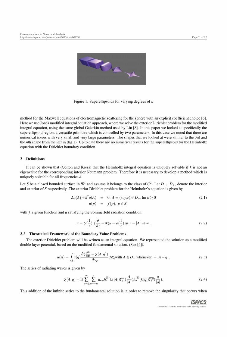
Figure 1: Superellipsoids for varying degrees of n

method for the Maxwell equations of electromagnetic scattering for the sphere with an explicit coefficient choice [6].Here we use Jones modified integral equation approach, where we solve the exterior Dirichlet problem for the modifiedintegral equation, using the same global Galerkin method used by Lin [8]. In this paper we looked at specifically thesuperellipsoid region, a versatile primitive which is controlled by two parameters. In this case we noted that there arenumerical issues with very small and very large parameters. The shapes that we looked at were similar to the 3rd andthe 4th shape from the left in (fig.1). Up to date there are no numerical results for the superellipsoid for the Helmholtzequation with the Dirichlet boundary condition.

2 Definitions

It can be shown that (Colton and Kress) that the Helmholtz integral equation is uniquely solvable if k is not aneigenvalue for the corresponding interior Neumann problem. Therefore it is necessary to develop a method which isuniquely solvable for all frequencies k.

Let S be a closed bounded surface in ℜ3 and assume it belongs to the class of C2. Let D−, D+, denote the interiorand exterior of S respectively. The exterior Dirichlet problem for the Helmholtz’s equation is given by

∆u(A)+ k2u(A) = 0, A = (x,y,z) ∈ D+, Im k ≥ 0 (2.1)u(p) = f (p), p ∈ S,

with f a given function and u satisfying the Sommerfeld radiation condition:

u = O(1r),(

∂∂ r

− ik)u = o(1r) as r = |A| → ∞. (2.2)

2.1 Theoretical Framework of the Boundary Value ProblemsThe exterior Dirichlet problem will be written as an integral equation. We represented the solution as a modified

double layer potential, based on the modified fundamental solution. (See [4]).

u(A) =∫

Su(q)

∂ ( eikr

4πr +χ(A,q))∂νq

dσqwith A ∈ D+ whenever = |A−q| . (2.3)

The series of radiating waves is given by

χ(A,q) = ik∞

∑n=0

n

∑m=−n

anmh(1)n (k |A|)Y mn (

A|A|

)h(1)n (k |q|)Y mn (

q|q|

). (2.4)

This addition of the infinite series to the fundamental solution is in order to remove the singularity that occurs when

International Scientific Publications and Consulting Services


A = q.

Here h(1)n denote the spherical Hankel function of the first kind and of order n, Y mn , n = −m, ...m are the linearly

independent spherical harmonics of order m given by Y mn (ϕ ,θ) = (

12π

(m+ 12 )(m−n)!(m+n)!

)12 pm

n (cosθ)eimϕ .

As in [4] here we assume that D− (superellipsoid) to be a connected domain containing the origin and we choose aball B of radius R and center at the origin such that B ⊂ D−. On the coefficients anm we imposed the condition thatthe series χ(p,q) is uniformly convergent in p and in q in any region |p| , |q| ≥ R+ ε , ε > 0, and that the series canbe two times differentiated term by term with respect to any of the variables with the resulting series being uniformlyconvergent. We also assumed that the series χ is a solution to the Helmholtz equation satisfying the Sommerfeldradiation condition for |p| , |q|> R. By letting A tend to a point p ∈ S, we obtain the following integral equation basedon the Fredholm equations of the second kind

−2πµ(p)+∫

Sµ(q)

∂Ψ(p,q)∂νq

dσq =−4π f (p), p ∈ S (2.5)

where

Ψ =−eikrqp

r−4πχ(p,q).

We denote the above integral equations by

−2πµ +Kµ =−4π f , (2.6)

where in the Dirichlet case

Kµ(p) =∫

Sµ(q)

∂∂νq

(−eikrqp

r−4πχ(p,q))dσq.

By the assumptions on the series χ(p,q) the kernel ∂ χ(p,q)∂νq

is continuous on S×S, and hence K is compact from C(S)

to C(S) and L2(S) to L2(S).

Kleinman and Roach [7] gave an explicit form of the coefficient anm that minimizes the upper bound on the spectralradius (see [6]). If B is the exterior of a sphere radius R with center at the origin then the optimal coefficient for theDirichlet problem was given by

anm =−12(

jn(kR)

h(1)n (kR)+

j′n(kR)

h(1)′

n (kR)) for n = 0,1,2 ... and m =−n, ... n.

This choice of the coefficient minimizes the condition number, and (2.6) is uniquely solvable for the superellipsoid.

This coefficient was given for spherical regions. Also the coefficient choice of anm =−12(

jn(kR)

h(1)n (kR)) was also consid-

ered but did not give good convergence results.



3 Smoothness of the integral operator K

Smoothness results of the double layer operator was proven by Lin [8]. We know that the series χ can be differ-entiated term by term with respect to any of the variables and that the resulting series is uniformly convergent. So thesecond derivative of the series is continuous on ℜ3\B where B = {x : |x| ≤ R}. Furthermore the series χ is a solutionto the Helmholtz equation satisfying the Sommerfeld radiation condition for |x| , |y| > R, when B = {x : |x| ≤ R} iscontained in D.

By (Theorem 3.5 [3]) any two times continuously differentiable solution of the Helmholtz’s equation is analytic,and analytic functions are infinitely differentiable. So the series χ(p,q) is infinitely differentiable with respectto any of the variables p,q. Furthermore it is easy to see that if µ is bounded and integrable and S ∈ Cl then∫

S χ(p,q)µ(q)dσq ∈Cl(S) and∫

S∂ χ(p,q)

∂νqµ(q)dσq ∈Cl(S).

4 The Framework of the Galerkin Method

The variable of integration in (2.6) was changed, converting it to a new integral equation defined on the unit sphere.The Galerkin method was applied to this new equation,using spherical polynomials to define the approximating sub-spaces. m : U →1−1

onto S, where m is at least differentiable.

By changing the variable of integration on (2.6) we obtained the new equation over U,

−2πµ̂ + K̂µ̂ =−4π f̂ , f̂ ∈C(U). (4.7)

The notation “ˆ” denotes the change of variable from S to U. The operator (−2π + K̂)−1 exists and is bounded onC(U) and L2(U). Let X = L2(U),α = −2π, and let an approximating subspace of spherical polynomials of degree≤ N be denoted by XN . The dimension of XN is dN = (N + 1)2 : and we let {h1, ...hd} denote the basis of sphericalharmonics Galerkin’s method for solving (4.7) for the Dirichlet boundary conditions is given by

(−2π +PNK̂)µ̂N =−4πPN f̂ . (4.8)

The solution is given by

µ̂N =d

∑j=1

α jh j

−2παi(hi,hi)+d

∑j=1

α j(K̂h j,hi) =−4π( f̂ ,hi), i = 1, ... d. (4.9)

The convergence of µN to µ in L2(S) is straightforward We know from previous literature that PN µ̂ → µ̂ for allµ̂ ∈ L2(U). From standard results it follows that

∥∥∥K̂ −PNK̂∥∥∥→ 0 and we can obtain the desired convergence.

(Also see [2]).Using the smoothness results of the integral operator K from section III, and following the same proofas in [1], we can prove the following theorems.

Theorem 4.1. Assume that f ∈ Cl,λ (S), S ∈ Cl+1,λ (S ∈ C2 for l = 0) and that the mapping m satisfies (4.7) forsome l ≥ 0. Then for all sufficiently large N, the inverses (−2π + PNK̂)−1 exist and are uniformly bounded and∥µ −µN∥ ≤

cNl+λ ′ where 0 < λ ′

< λ is arbitrary. The constant c depends on l,µ, and λ ′.

Convergence in C(U). To prove uniform convergence of µ̂N to µ̂ is slightly more difficult. The main problem is thatthere are µ̂ in C(U) for which PN µ̂ does not converge to µ̂. Convergence for all µ̂ would imply uniform boundednessof ∥PN∥.



Theorem 4.2. Assume that S ∈C2 and that m satisfies (4.7) with l = 0. Then considering K̂ as an operator on C(U),∥∥∥K̂ −PNK̂∥∥∥→ 0 as N → ∞. (4.10)

This implies the existence and uniform boundedness on C(U) of (−2π + PNK̂)−1 for all sufficiently large N. Let(−2π + K̂)µ̂ = −4π f̂ and (−2π +PNK̂)µ̂N = −4πPN f̂ . If f ∈ C0,λ (S), λ > 1

2 , then µ̂N converges uniformly to µ̂.

Moreover, if S ∈Cl+1,λ (S ∈C2, for l = 0) and f ∈Cl,λ (S), l +λ > 12 , then ∥µ −µN∥∞ ≤ C

Nl+λ ′− 12

with 0 < λ ′ < λ .

The constant c depends on f , l,λ ′.

4.1 The approximation of true solutions for the Dirichlet problemGiven µN an approximate solution of (2.6), we defined the approximate solution uN of (2.1) using the integral

(2.3).

uN(A) =∫

SµN(q)

∂∂υq

(eikrqA

4πrqA+χ(A,q))dσq,A ∈ D+. (4.11)

To show the convergence of uN(A), we used the following lemma.

Lemma 4.1.

Asup∈ K

∫S

∣∣∣∣ ∂∂νq

(eikrqA

4πrqA+χ(A,q))

∣∣∣∣dσq < ∞, (4.12)

where K is any compact subset of D, from Warnapala and Morgan [10].

4.2 Implementation of the Galerkin Method for the Dirichlet ProblemThe coefficients (K̂h j,hi) are fourfold integrals with a singular integrand. Because the Galerkin coefficients

(K̂h j,hi) depends only on the surface S, we calculated them separately for N ≤ Nmax. The following derivation wasdone for the Dirichlet problem. To decrease the effect of the singularity in computing K̂h j(p̂) in the Dirichlet case,we used the identity ∫

S− ∂

∂νq

1rqp

dσq = 2π, p ∈ S where rqp = |p−q| ,

to write ∫S− ∂

∂νq

1rqp

dσq = 2π, p ∈ S where rqp = |p−q| ,∫

U−(h j(q̂)−h j(p̂)

∂̂∂νq

1rqp

|J(q̂)|dσq̂.

The integrands are bounded at q̂ = p̂, where J(q̂) is the Jacobian.

5 Numerical Examples/Experimental Surfaces

In this section, several numerical examples are presented. The true solutions is given by

u1(x,y,z) =eikr

r.

The parametric equation for the superellipsoid is given by f (x,y) = (cos(x)sin(y)n, sin(x)sin(y)n,cos(y)) where nvaried from 0.5 to 4. The surface area of the superellipsoid has no closed form, thus one cannot give a specific

formula but the volume is given by8(Γ(1+ 1

n ))3

Γ(1+ 1n )

. For analysis it is important to realize that the superellipsoid is

simply connected and is of infinite extent.



Figure 2: The superellipsoid for n = 4

In our tables INN are the interior nodes for calculating K̂h j, EXN are the exterior nodes needed for calculating(K̂h j,hi) and NINT are the nodes for calculating uN . N denotes the degree of the approximate spherical harmonics,recall that the number d of basis functions equals to (N + 1)2. In most cases we only added a few terms from theseries. According to Jones [5] this is sufficient to remove the corresponding interior Dirichlet eigenvalues and obtainunique solutions at the same time.

The following Numerical results were obtained for the Dirichlet problem.



Figure 3: The superellipsoid for n = 3

Figure 4: The superellipsoid for n = 0.5



Table 1

k = 1, n = 3, N = 7, INN = 32, EXN = 16, true solution u1

point absolute error

5,6,7 2.86D−0610,11,13 2.003D−0623,22,45 1.323D−0723,43,56 3.143D−07

In all the examples we used the coefficient anm.

Table 2

k = 1, n = 4, N = 7, INN = 32, EXN = 16, true solution u1


5,6,7 7.829D−0610,11,12 4.500D−0621,22,23 2.494D−0634,12,32 1.070D−06

When we made the k value smaller, we obtained the following Table 3(a).

Table 3(a)

k = 0.01, n = 3, N = 7, INN = 32, EXN = 16,2nd boundary condition true solution u1


5,6,7 7.723D−0510,11,12 2.229D−0520,21,22 6.194D−0623,43,12 1.353D−06

As you can see from the above Table 3(a) the results were mostly worse compared to the Table 1. Now wedecreased the n value and made the k value an eigenvalue of the corresponding interior Neumann problem, andobtained Table 3(b).

Table 3(b)

k = 4.493409, n = 1.4, N = 7, INN = 32, EXN = 16,number of terms 10, true solution u1


10,11,12 3.703D−0514,12,16 6.715D−0523,21,23 3.328D−0545,32,34 5.078D−05



From Table 3(b) it is evident that our method is successful as we get good convergence results for the eigenvalueof the interior Neumann problem. We also added more than five terms and still obtained good results. But as moreterms and increasing of integration nodes, increases the CPU time considerably (this will be discussed later moreextensively), we added only a few terms, only five in other cases of superellipsoid. In the next tables we changed then values.

Table 4

k = 0.001, n = 3, N = 7, INN = 32, EXN = 16, true solution u1


5,6,7 9.351D−0810,11,12 8.440D−0820,24,36 3.548D−0812,43,23 3.504D−08

From Table 1, 2, 3(a), 3(b) and Table 4, we see that for the points away from the boundary there is much greateraccuracy than for points near the boundary. This is because the integrand is more singular at points near the boundary.

Table 5

k = 0.01, n = 1.4, N = 7, INN = 32, EXN = 16, true solution u1


1,2,3 2.372D−065,6,7 9.680D−07

10,11,12 5.299D−0720,21,22 2.805D−07

From Table 5 we see that to obtain similar accuracy as in the previous tables we might need to decrease the nvalue. This is due to the following fact: the superellipsoidal shape looks more spherical when the n value decreases.

Remark 5.1. We picked EXN < INN, because the integrand of (hi, K̂h j) is smoother than the integrand of K̂h j. Wealso picked EXN ≥ (N +1).

More numerical data for varying values of n.



Table 6

k = 0.01, n = 2, N = 7, INN = 32, EXN = 16, true solution u1


1,2,3 9.271D−0610,11,12 1.646D−0620,21,23 8.486D−0734,23,54 4.632D−07

Table 7



1,2,3 9.971D−065,6,7 3.171D−06

10,11,12 1.735D−0620,21,22 8.94D−07

Table 8



1,2,3 2.789D−065,6,7 7.376D−07

10,11,12 4.031D−0723,34,32 1.480D−07

When n is changed, we obtained new shapes of superellipsoids. When we increased the nodes we obtained betterresults for relatively smaller n values.



Figure 5: Further the points are from the boundary better the convergence results

The (Fig.5) shows that further the points are from the boundary the better the convergence results are for thisproblem, which is the expected result.

Remark 5.2. Few terms from the infinite series were added in all our numerical experiments. This is because innumerical calculations it is inefficient to add the full series. So we allow only a finite number of the coefficients anmto be different from zero. According to Jones [5], this is sufficient to ensure uniqueness for the modified integralequations in a finite range of wave numbers k. In practical applications, one is usually concerned with a finite rangeof k so this is not a serious draw back. In order to use a large amount of nodes we need a considerably high amountof CPU time. From the above examples, we see that the error is effected by the boundary S, INN, EXN, boundarydata and k and n. As the value of the n decreases the ellipsoidal nature of the superellipsoid for the Dirichlet problemincreases and the rate of convergence decreases. If we want to obtain more accuracy, we must increase the number ofintegration nodes for calculating the Galerkin coefficients (K̂h j,hi). The cost of calculating the Galerkin coefficientsis high. Some of the increased cost comes from the complex number calculations, which is an intrinsic property ofthe Helmholtz equation. Furthermore any integration method is affected by k, due to the oscillatory behavior of the

fundamental solutioneikr

r. Also the CPU time depends on the number of terms added from the series.

In order to eliminate more interior Neumann eigenvalues we need a more powerful computer which would decreasethe CPU time considerably. We also see that for the shapes of superellipsoid with small n values the convergenceresults are extremely good, even though the coefficient choice that was used was originally designed for sphericalregions.

Acknowledgements

We would like to thank Dr. Rutherford and Mrs. Kennedy for their technical support in getting this paper ready. Theauthor is grateful to the anonymous referees for their comments which substantially improved the quality of this paper.



References

[1] K. E. Atkinson, The numerical solution of the Laplace’s equation in three dimensions, SIAM J. Numer. Anal, 19(1982) 263-274.http://dx.doi.org/10.1137/0719017

[2] K. E. Atkinson, The Numerical Solution of Integral Equations of the Second Kind, Cambridge University Press,(1998).

[3] David Colton, Rainer Kress, Integral equation methods in scattering theory, (1983).

[4] C. Criado, N. Alamo, Thomas rotation and Foucault pendulum under a simple unifying geometrical point of view,Int. J. Non-Linear Mech, 44 (2009) 923-927.http://dx.doi.org/10.1016/j.ijnonlinmec.2009.06.008

[5] D. S. Jones, Integral equations for the exterior acoustic problem, Q. J. Mech. Appl. Math, 27 (1974) 129-142.http://dx.doi.org/10.1093/qjmam/27.1.129

[6] G. Jost, Integral equations with Modified Fundamental Solution in Time-Harmonic Electromagnetic Scattering,IMA J. Appl. Math, 40 (1988) 129-143.http://dx.doi.org/10.1093/imamat/40.2.129

[7] R. E. Kleinman, G. F. Roach, On modified Green functions in exterior problems for the Helmholtz equation, Proc.R. Soc. Lond. A, 383 (1982) 313-333.http://dx.doi.org/10.1098/rspa.1982.0133

[8] T. C. Lin, The numerical solution of Helmholtz equation using integral equations, Ph.D. thesis, University ofIowa, Iowa City, Iowa, (1982),

[9] T. C. Lin, Y. Warnapala-Yehiya, The Numerical Solution of the Exterior Dirichlet Problem for Helmholtz’s Equa-tion via Modified Green’s Functions Approach, Comput. Math. Appl, 44 (2002) 1229-1248.http://dx.doi.org/10.1016/S0898-1221(02)00229-8

[10] Y. Warnapala, E. Morgan, The Numerical Solution of the Exterior Dirichlet Problem for Helmholtz’s Equationvia Modified Green’s Functions Approach for the Oval of Cassini, Far East J. Appl. Math, 34 (2009) 1-20.


Date post:	11-Feb-2022
Category:	Documents
Upload:	others
View:	2 times
Download:	0 times

Numerical solution of the helmholtz equation for the superellipsoid via the galerkin method

Documents