Abstract— A numerical method based on Legendre wavelets

is proposed for fractional partial differential equations.

Legendre wavelets operational matrices of fractional order

integration and fractional order differentiation are derived. By

using these matrices, each term of the problem was converted

into matrix form. Lastly, the equation was transformed into a

Sylvester equation. The error estimation of the Legendre

wavelets method is given in Theorem 5.1. Three numerical

examples are shown to demonstrate the validity and

applicability of the method.

Index Terms— Fractional partial differential equation,

Legendre wavelets, Operational matrix, Sylvester equation,

Error analysis

I. INTRODUCTION

N science and engineering, many dynamical systems can

be described by fractional-order equations [1-3]. These

dynamical systems generally originates in the fields of

electrode-electrolyte [4], dielectric polarization [5],

electromagnetic waves [6], viscoelastic systems [7] etc.

Various materials and processes have been found to be

described using fractional calculus. Anomalous diffusion has

been discussed in various physical fields [8-10]. The features

of anomalous diffusion include history dependence,

long-range correlation and heavy tail characteristics. These

features can be accommodated well by using fractional

calculus. In order to model these phenomena, fractional

derivatives and fractional partial differential equations were

proposed. Nowadays, fractional partial differential equations

have been employed as a powerful tool in complex

anomalous diffusion modelling.

Apart from modelling aspects of these fractional partial

differential equations, the numerical solution techniques are

rather more significant aspects. Various numerical methods

and approaches are available to solve linear and nonlinear

fractional partial differential equations. Some analytic

Manuscript received January 16, 2016; revised June 22, 2016.

Hao Song is with the School of Aeronautic Science and Engineering,

Beihang University, Beijing, P.R.China (e-mail: buaasonghao@163.com).

Mingxu Yi (Corresponding author) is with the School of Aeronautic

Science and Engineering, Beihang University, Beijing, P.R.China (e-mail:

yimingxu88@163.com).

Jun Huang is with the School of Aeronautic Science and Engineering,

Beihang University, Beijing, P.R.China

Yalin Pan is with the School of Aeronautic Science and Engineering,

Beihang University, Beijing, P.R.China

methods are proposed. However, numerical methods are in

demand since it is difficult to obtain analytic solutions for

each and every fractional partial differential equation

originating from real life problems. Until now, to the best of

the author’s knowledge, the main approach for solving

fractional partial equations were the finite difference method

[11, 12], Laplace transform method [13], and generalized

differential transform method [14]. These approximations are

valuable for researchers and scientists.

This research considered a class of fractional partial

equations:

( , )u u

f x yx y

. (1)

such that

(0, ) ( ,0) 0u y u x . (2)

where ( , )u x y x and ( , )u x y y are fractional

derivatives, ( , )f x y is the known continuous function,

( , )u x y is the unknown function, and 0 , 1 .

II. LEGENDRE WAVELETS

Legendre wavelets ( )nm x are expressed as follows [15]

1/2

2ˆ ˆ2 1 1 1

ˆ2 (2 ), ;( ) 2 2 2

0, .

k

k

m k knm

m n nP x n x

x

otherwise

（3）

where 1,2, ,k ˆ 2 1n n , 11,2, ,2kn ,

0,1, , 1m M is the degree of the Legendre polynomials

and M is a fixed positive integer; ( )mP x are Legendre

polynomials of degree m .

For any function, 2( ) [0,1)f x L may be given by the

Legendre wavelets as

1 0

( ) ( )nm nm

n m

f x c x

. (4)

where ( ), ( )nm nmc f x x , and , is the inner product of

( )f x and ( )nm x .

If the infinite series in Equation (4) is truncated, then 12 1

1 0

( ) ( ) ( ).

k MT

nm nm

n m

f x c x C x

(5)

where C and ( )x are 1ˆ 2km M column vectors

1 1 1

10 11 1 1 20 21

2 1 2 0 2 1 2 1

[ , , , , , , ,

, , , , , ] .k k k

M

T

M M

C c c c c c

c c c c

(6)

Numerical Solutions of Fractional Partial

Differential Equations by Using Legendre

Wavelets

Hao Song, Mingxu Yi*, Jun Huang, and Yalin Pan

I

Engineering Letters, 24:3, EL_24_3_17

(Advance online publication: 27 August 2016)

______________________________________________________________________________________

1 1 1

10 11 1 1 20 21

2 1 2 0 2 1 2 1

( ) [ , , , , , , ,

, , , , , ] .k k k

M

T

M M

x

(7)

For simplicity, Equation (5) is rewritten as ˆ

1

( ) ( ) ( ).m

T

i i

i

f x c x C x

(8)

where i nmc c ,

i nm . The index i is determined by the rel

-ation ( 1) 1i M n m .

Therefore, the vectors can also be written as

1

1 2 1

ˆ2 (2 1) 1

[ , , , , , ,

, , , , ] .k

M M

T

M mM

C c c c c

c c c

(9)

1

1 2 1

ˆ2 (2 1) 1

( ) [ , , , , , ,

, , , , ] .k

M M

T

M mM

x

(10)

Similarly, the function ( , )u x y over [0,1) [0,1) can be

expressed as follows ˆ ˆ

1 1

( , ) ( ) ( ) ( ) ( ).m m

T

ij i j

i j

u x y u x y x U y

(11)

where [ ]ijU u and ( ), ( , ), ( )ij i ju x u x y y .

Theorem 2.1[16] Any function ( )f x , defined over [0,1] , is with

bounded second derivative, say ( )f x M , can be expressed

as the sum of Legendre wavelets, and the series converges

uniformly to the function ( )f x .That is

1 0

( ) ( ).nm nm

n m

f x c x

where ( ), ( )nm nmc f x x , and , is the inner product of

( )f x and ( )nm x .

Theorem 2.2[17]

If a continuous function ( , )u x y defined over

[0,1) [0,1) has bounded mixed fourth partial

derivative4

2 2

( , )u x yM

x y

, then the Legendre wavelets

expansion of ( , )u x y converges uniformly to it.

III. OPERATIONAL MATRICES OF INTEGRATION AND

DIFFERENTIATION FOR LEGENDRE WAVELETS

3.1 Fractional Calculus

Definition 1. The Riemann-Liouville fractional integral

operator of order 0 of a function is defined as [13]

1

0

1( ) ( ) ( ) , 0.

( )

x

J f x x f d

(12)

0 ( ) ( ).J f x f x (13)

Definition 2. The fractional differential operator in Caputo

sense is defined as

( )

10

( ), ;

( )1 ( )

, 0 1 .( ) ( )

r

r

rx

r

d f xr N

dxD f x

fd r r

r x

(14)

The Caputo fractional derivative of order is also given

by ( ) ( )r rD f x J D f x , where rD is the usual integer

differential operator of order r . The relation between the

Caputo operator and Riemann-Liouville operator is given as

follows:

( ) ( ).D J f x f x (15)

1( )

0

( ) ( ) (0 ) , 0.!

krk

k

xJ D f x f x f x

k

(16)

3.2 Fractional Order Operational Matrix of Integration and

Differentiation for Legendre Wavelets.

This section simply presents the operational matrix of

fractional integration of Legendre wavelets [15].

Firstly, the basis set of block pulse functions is

considered. These functions, defined over [0,1) , are given as

follows [18]

1, ( 1) ;( )

0, .i

ih x i hb x

otherwise

(17)

Note: ˆ0,1,2, , 1i m and is a positive integer value for

m̂ and 1

ˆh

m .

Let ˆ0 1 1( ) [ ( ), ( ), , ( )]T

mB x b x b x b x . Accordingly, suppose

( ) ( ).J B x F B x (18)

where F is the fractional integration block pulse operationa

l matrix [18], where

ˆ1 2 1

ˆ1 2

ˆ 3

1

0 11

.0 0 1( 2)

0 0 0 1

m

m

mF h

Here, 1 1 1( 1) 2 ( 1)k k k k , ˆ1,2, , 1k m .

There is a relationship between the Legendre wavelets and

block pulse functions [19]

( ) ( ).x B x (19)

where ˆ0 1 1[ ( ), ( ), , ]mx x ,ˆ

i

ix

m , ˆ0,1, , 1i m .

Legendre wavelets fractional integration operator J satisfies

( ) ( ).J x P x (20)

where P is the Legendre wavelets fractional integration

operational matrix . Equation (18) and Equation (19) result in

( ) ( ) ( ) ( ).J x J B x J B x F B x (21)

Using Equation (20) and Equation (21),

( ) ( ) ( ).P x P B x F B x (22)

Then, matrix P is as follows 1.P F (23)

The fractional derivative of order in the Caputo sense of

the vector ( )x can be expressed as

( ) ( ).D x Q x (24)

where Q is the ˆ ˆm m Legendre wavelets operational matrix

of fractional differentiation. Due to the relationship in

fractional calculus, Q P I , matrix Q can easily be

acquired by inverting matrix P .

The fractional order integration and differentiation of the

function t are selected to verify the effectiveness of matrix

P and Q . The fractional order integration and

differentiation of ( )u t t are obtained as follows:

1(2)( )

( 2)J u t t

and 1-(2)( )

(2- )D u t t

.

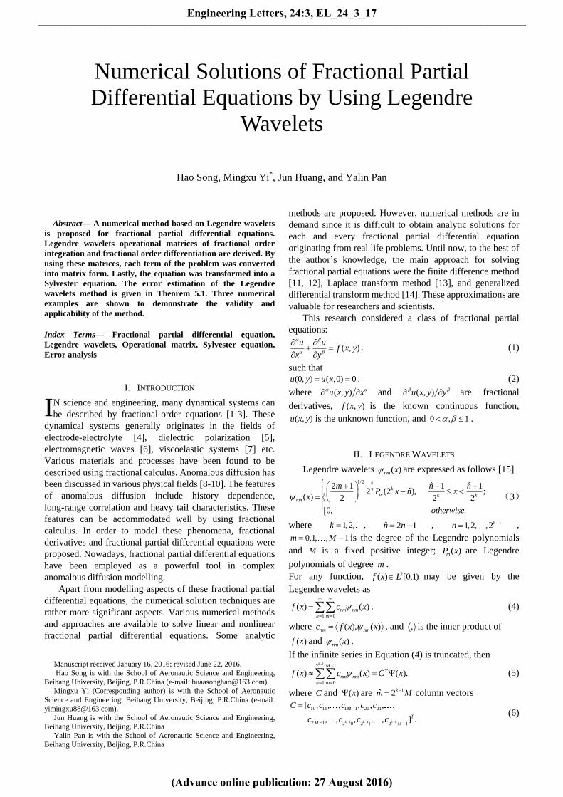
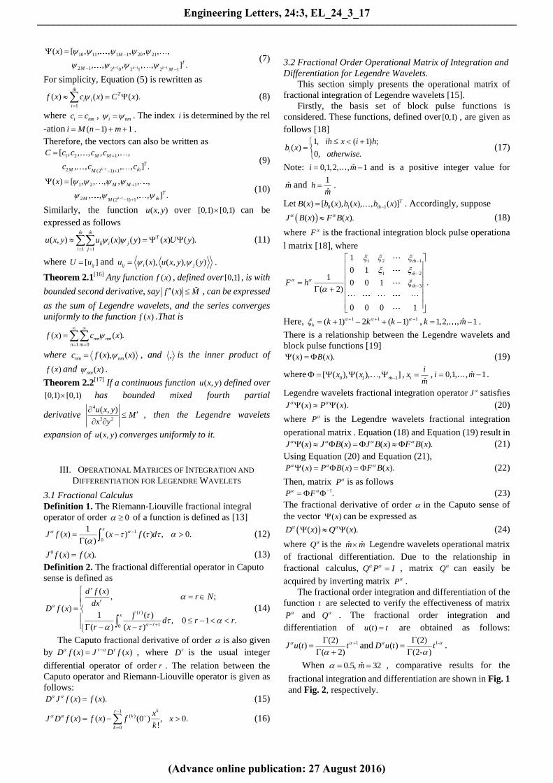
When ˆ0.5, 32m , comparative results for the

fractional integration and differentiation are shown in Fig. 1

and Fig. 2, respectively.

Engineering Letters, 24:3, EL_24_3_17

(Advance online publication: 27 August 2016)

______________________________________________________________________________________

Fig. 1. 1/2 order integration of ( )u t t .

Fig. 2. 1/2 order differentiation of ( )u t t .

IV. SOLUTION OF THE FRACTIONAL PARTIAL DIFFERENTIAL

EQUATION

Consider the fractional partial differential equation

Equation (1) in section 1. If it is assumed the function

( , )u x y in terms of Legendre series, it can be written as

Equation (11).

Then the following can be obtained:

( ( ) ( )) ( )( )

[ ( )] ( ) ( )[ ] ( ).

TT

T T T

u x U y xU y

x x x

Q x U y x Q U y

(25)

( ( ) ( ))

( ( ))( ) ( ) ( ).

T

T T

u x U y

y y

yx U x UQ y

y

(26)

The function ( , )f x y of Equation (1) may also be written as

( , ) ( ) ( ).Tf x y x F y (27)

where ˆ ˆ,[ ]i j m mF f .

Substituting Equation (25), Equation (26) and Equation (27)

into Equation (1), then

( )[ ] ( ) ( ) ( )

( ) ( ).

T T T

T

x Q U y x UQ y

x F y

(28)

Dispersing Equation (28) by points ( , )i jx y ,

ˆ1,2, ,i m and ˆ1,2, ,j m , then

[ ] .TQ U UQ F (29)

Equation (28) is a Sylvester equation. The Sylvester equation

can be solved easily using Matlab2011a.

V. ERROR ANALYSIS

In this part, error analysis of the method is employed. Let

ˆ ( , )mu x y

x

be the following approximation

of( , )u x y

x

,

ˆ ˆˆ

1 1

( , )( ) ( )

m mm

ij i j

i j

u x yu x y

x

.

Then ˆ

ˆ ˆ1 1

( , ) ( , )( ) ( )m

ij i j

i m j m

u x y u x yu x y

x x

.

Theorem 5.1 Let the function ˆ ( , )mu x y

x

obtained using

Legendre wavelets be the approximation of( , )u x y

x

, and

( , )u x y has bounded mixed fractional partial

derivative4

2 2

( , ) ˆu x yM

x y

, then

1/ 2

ˆ

4

ˆ ˆ( , ) ( , )

2

m

k

E

u x y u x y M N

x x

,

wher 1/2

1 12

0 0( ) ( )

Eu x,y u x,y dxdy ,

( , )( ), , ( )ij i j

u x yu x y

x

, and N̂ is a constant.

Proof.

The orthonormality of the series ( )i x , defined on [0,1) ,

implies1

0( )[ ( )]Tx x dx I , where I is the identify matrix,

then 2

ˆ

21 1

ˆ

0 0

21 1

0 0ˆ ˆ1 1

1 1 1 1

0 0 0 0ˆ ˆ ˆ ˆ1 1 1 1

( , ) ( , )

( , ) ( , )

( ) ( )

= ( ) ( ) ( ) ( )

m

E

m

ij i j

i m j m

ij i j i j i j

i m j m i m j m

u x y u x y

x x

u x y u x ydxdy

x x

u x y dxdy

u u x y dxdy x y dx

1 12 2 2

0 0ˆ ˆ1 1

2

ˆ ˆ1 1

( ) ( )

.

ij i j

i m j m

ij

i m j m

dy

u x dx y dy

u

The Legendre wavelets coefficients of function ( , )u x y are

defined by 1 1

0 0

1/21

/2

0

( , )( ) ( )

( , ) 2 1ˆ2 (2 ) ( ) .

2nk

ij i j

k k

m jI

u x yu x y dxdy

x

u x y mP x n y dxdy

x

Let ˆ2k x n t .By changing ˆ2k x n t and1

2kdx dt , then

Engineering Letters, 24:3, EL_24_3_17

(Advance online publication: 27 August 2016)

______________________________________________________________________________________

1/21 1

/2

0 1

1/2

1

1 1

1 10 1

1/2

3 1

11

11

ˆ2 12 ( ) , ( )

2 2

1

2 (2 1)

ˆ( ) , ( ( ) ( ))

2

1

2 (2 1)

ˆ( ) , (

2

ij

k

j mk

k

j m mk

k

j mk

u

m n ty u y P t dtdy

t

m

n ty u y d P t P t dy

t

m

n ty u y P

t

1

1 10

1/2

3 1

11 1

2 2

10 1

1/2

5 1

21

2

21

( ) ( ))

1=

2 (2 1)

ˆ ( ) ( ) ( ) ( )( ) ,

2 2 3 2 1

1

2 (2 1)

ˆ ( ) ( )( ) ,

2 2 3

m

k

m m m mj k

k

m m mj k

t P t dtdy

m

P t P t P t P tn ty u y d dy

t m m

m

P t P t Pn ty u y

t m

1

2

0

( ) ( ).

2 1

mt P tdtdy

m

Now,

let2 2( ) (2 1) ( ) 2(2 1) ( ) (2 3) ( )m m m mt m P t m P t m P t ,

then 1/2

5 1

21 1

20 1

1 1

2 (2 1) (2 1)(2 3)

ˆ( ) , ( ) .

2

ij k

j mk

um m m

n ty u y t dtdy

t

By solving this equation, 4

1 1

2 21 1

ˆ ˆ( , ) , ( ) ( ) .

2 2ij m mk k

n t n su A k m u t s dtds

t s

where 5 1 2 2

1 1( , ) .

2 (2 1) (2 1) (2 3)kA k m

m m m

Therefore 4

1 1

2 21 1

ˆ ˆ( , ) , ( ) ( ) .

2 2ij m mk k

n t n su A k m u t s dtds

t s

Furthermore, the above equation reveals 1

1

2 3( ) 24 .

2 3m

mt dt

m

Thus, 2

5 2 5 4

ˆ24 (2 3)( , )

2 3

ˆ1 1 12.

2 (2 1) (2 3)(2 1) (2 ) (2 3)

ij

k

M mu A k m

m

M

m m m n m

Namely, 2

2

10 8

ˆ144.

(2 ) (2 3)ij

Mu

n m

Therefore,

1 1

1 1

2

ˆ

22

10 8ˆ ˆ ˆ ˆ

2 2

10 8 10 8ˆ ˆ 2 2

22 1 2 1

10 8

2 2

( , ) ( , )

ˆ144

(2 ) (2 3)

ˆ ˆ144 144

(2 ) (2 5) (2 ) (2 5)

ˆ144

(2 ) (2 5)

k k

p p

p p

m

E

ij

i m j m i m j m

k ki m j m i M j M

M M

k

i M j M

u x y u x y

x x

Mu

n m

M M

M M

M

M

1 1

2 22 2

1 10 8 1 81 1

ˆ ˆ ˆ1442 .

(2 ) (2 5) 2

M p k

p

p kM p k

M M NM

M

where N̂ is a constant.

Next, 2

2

ˆ

8

ˆ ˆ( , ) ( , )

2

m

k

E

u x y u x y M N

x x

.

Thus

1/ 2

ˆ

4

ˆ ˆ( , ) ( , )

2

m

k

E

u x y u x y M N

x x

.

From this theorem, it is evident

ˆ( , ) ( , )0m

E

u x y u x y

x x

when k .

VI. NUMERICAL EXAMPLES

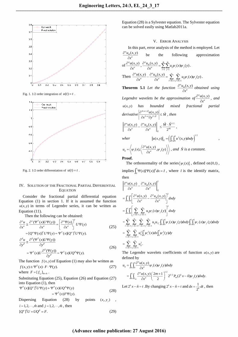
Example 1. Consider the nonhomogeneous partial

differential equation 1/5 1/5

1/5 1/5+ ( , ), , 0.

u uf x y x y

x y

Such that (0, ) ( ,0) 0u t u x and4/5 4/55( )

( , )4 (4 / 5)

x y xyf x y

. The

numerical results for ˆ 8m , ˆ =16m , ˆ =32m are shown in Fig. 3,

Fig. 4, Fig. 5. The exact solution is xy , shown in Fig. 6. Fig.

3-6 illustrate the numerical solutions are in very good

coincidence with the exact solution.

Fig. 3. Numerical solution of ˆ 8m .

Engineering Letters, 24:3, EL_24_3_17

(Advance online publication: 27 August 2016)

______________________________________________________________________________________

Fig. 4. Numerical solution of ˆ 16m .

Fig. 5. Numerical solution of ˆ 32m .

Fig. 6. Exact solution for Example 1.

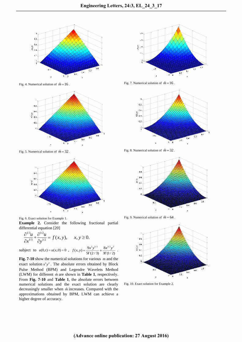
Example 2. Consider the following fractional partial

differential equation [20] 1/3 1/2

1/3 1/2+ ( , ), , 0.

u uf x y x y

x y

subject to (0, ) ( ,0) 0u t u x , 2 5/3 3/2 29 8

( , )5 (2 / 3) 3 (1/ 2)

x y x yf x y

.

Fig. 7-10 show the numerical solutions for various m and the

exact solution 2 2x y . The absolute errors obtained by Block

Pulse Method (BPM) and Legendre Wavelets Method

(LWM) for different m̂ are shown in Table 1, respectively.

From Fig. 7-10 and Table 1, the absolute errors between

numerical solutions and the exact solution are clearly

decreasingly smaller when m̂ increases. Compared with the

approximations obtained by BPM, LWM can achieve a

higher degree of accuracy.

Fig. 7. Numerical solution of ˆ 16m .

Fig. 8. Numerical solution of ˆ 32m .

Fig. 9. Numerical solution of ˆ 64m .

Fig. 10. Exact solution for Example 2.

Engineering Letters, 24:3, EL_24_3_17

(Advance online publication: 27 August 2016)

______________________________________________________________________________________

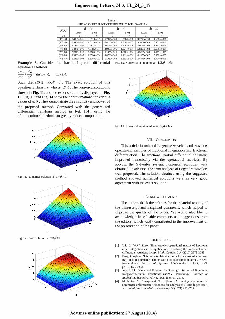
TABLE 1

THE ABSOLUTE ERROR OF DIFFERENT m FOR EXAMPLE 2

( , )x y ˆ 8m ˆ 16m ˆ 32m

LWM BPM LWM BPM LWM BPM

(0,0) 0 0 0 0 0 0

(1/8,1/8) 7.4931e-006 3.0719e-005 5.2376e-008 6.3969e-006 3.2276e-010 1.6065e-006

(2/8,2/8) 3.3456e-006 1.0113e-004 6.4260e-007 2.5382e-005 5.3431e-009 6.4515e-006

(3/8,3/8) 2.1453e-005 2.2617e-004 3.6551e-007 5.7263e-005 7.0156e-009 1.4572e-005

(4/8,4/8) 5.4356e-005 4.0185e-004 4.0276e-006 1.0214e-004 5.8820e-008 2.5983e-005

(5/8,5/8) 7.2573e-005 6.2905e-004 6.1355e-006 1.6009e-004 6.3285e-008 4.0692e-005

(6/8,6/8) 9.3462e-005 9.0799e-004 8.8762e-006 2.3113e-004 4.1455e-007 5.8709e-005

(7/8,7/8) 1.2653e-004 1.2388e-003 1.1992e-005 3.1532e-004 2.4376e-006 8.0040e-005

Example 3. Consider the fractional partial differential

equation as follows

+ sin( ), , 0.u u

x y x yx y

Such that (0, ) ( ,0) 0u t u x . The exact solution of this

equation is sin sinx y when = =1 . The numerical solution is

shown in Fig. 11, and the exact solution is displayed in Fig.

12, Fig. 13 and Fig. 14 show the approximations for various

values of , . They demonstrate the simplicity and power of

the proposed method. Compared with the generalized

differential transform method in Ref. [14], using the

aforementioned method can greatly reduce computation.

Fig. 11. Numerical solution of = =1 .

Fig. 12. Exact solution of = =1 .

Fig. 13. Numerical solution of =1/2, =1/3 .

Fig. 14. Numerical solution of =3/7, =3/5 .

VII. CONCLUSION

This article introduced Legendre wavelets and wavelets

operational matrices of fractional integration and fractional

differentiation. The fractional partial differential equations

improved numerically via the operational matrices. By

solving the Sylvester system, numerical solutions were

obtained. In addition, the error analysis of Legendre wavelets

was proposed. The solution obtained using the suggested

method showed numerical solutions were in very good

agreement with the exact solution.

ACKNOWLEDGMENTS

The authors thank the referees for their careful reading of

the manuscript and insightful comments, which helped to

improve the quality of the paper. We would also like to

acknowledge the valuable comments and suggestions from

the editors, which vastly contributed to the improvement of

the presentation of the paper.

REFERENCES

[1] Y.L. Li, W.W. Zhao, “Haar wavelet operational matrix of fractional

order integration and its applications in solving the fractional order

differential equations”, Appl. Math. Comput, 216 (2010) 2276-2285.

[2] Feng, Qinghua, “Interval oscillation criteria for a class of nonlinear

fractional differential equations with nonlinear damping term”, IAENG

International Journal of Applied Mathematics, vol.43, no.3,

pp154-159, 2013.

[3] Asgari, M, “Numerical Solution for Solving a System of Fractional

Integro-differential Equations”, IAENG International Journal of

Applied Mathematics, vol.45, no.2, pp85-91, 2015.

[4] M. Ichise, Y. Nagayanagi, T. Kojima, “An analog simulation of

noninteger order transfer functions for analysis of electrode process”,

Journal of Electroanalytical Chemistry, 33(1971) 253- 265.

Engineering Letters, 24:3, EL_24_3_17

(Advance online publication: 27 August 2016)

______________________________________________________________________________________

[5] H.H. Sun, A.A. Abdlwahad, B. Onaral, “Linear approximation of

transfer function with a pole of fractional order”, IEEE Transactions on

Automatic Control, 29(1984) 441-444.

[6] Borhani A, Pätzold M, “On the spatial configuration of scatterers for

given delay-angle distributions”, Engineering Letters, vol.22, no.1,

pp34-38, 2014.

[7] R.C. Koeller, “Application of fractional calculus to the theory of

viscoelasticity”, Journal of Applied Mechanics, 51 (1984) 299-307.

[8] Wang Y, Song W, Guo Q, et al. “Correction Mechanism Analysis for a

Class of Spin-stabilized Projectile with Fixed Canards”, Engineering

Letters, vol.23, no.4, pp269-276, 2015.

[9] W. Chen, “A speculative study of 2/3-order fractional Laplacian

modeling of turbulence: Some thoughts and conjectures”, Chaos, 16

(2006) 023126.

[10] H.G. Sun, W. Chen, H. Sheng, Y.Q. Chen, “On mean square

displacement behaviors of anomalous diffusions with variable and

random order”, Physics Letter A, 374 (2010) 906-910.

[11] P. Zhuang, F. Liu, V. Anh, I. Turner. “Numerical methods for the

variable-order fractional advection-diffusion equation with a nonlinear

source term”, SIAM J. Numer. Anal, 47 (2009) 1760- 1781.

[12] C. Chen, F. Liu, V. Anh, I. Turner, “Numerical schemes with high

spatial accuracy for a variable-order anomalous subdiffusion

equation”, SIAM J. Sci. Comput, 34 (4) (2010) 1740-1760.

[13] I. Podlubny, Fractional Differential Equations, Academic press, 1999.

[14] Zaid Odibat, Shaher Momani, “A generalized differential transform

method for linear partial differential equations of fractional order”,

Applied Mathematics Letters, 21 (2008) 194-199.

[15] H. Jafari, S.A. Yousefi, “Application of Legendre wavelets for solving

fractional differential equations”, Computers and Mathematics with

Application, 62(3) (2011) 1038-1045.

[16] N. Liu, E.B. Lin, “Legendre wavelet method for numerical solutions of

partial differential equations”, Numerical Methods for Partial

Differential Equations, 26 (2010) 81-94.

[17] M.H. Heydari, M.R. Hooshmandasl, F. Mohammadi, “Legendre

wavelets method for solving fractional partial differential equations

with Dirichlet boundary conditions”, Applied Methematics and

Computation, 234 (2014) 267-276.

[18] Y.L. Li, N. Sun, “Numerical solution of fractional differential

equations using the generalized block pulse operational matrix”,

Comput. Math. Appl, 62 (2011) 1046 -1054.

[19] M. ur Rehman, R. Ali Khan, “The Legendre wavelet method for

solving fractional differential equations”, Commun. Nonlinear Sci.

Numer. Simulat, 16 (2011) 4163-4173.

[20] M.X. Yi, J. Huang, J.X. Wei, “Block pulse operational matrix method

for solving fractional partial differential equation”, Applied

Methematics and Computation, 221 (2013) 121-131.

Engineering Letters, 24:3, EL_24_3_17

(Advance online publication: 27 August 2016)

______________________________________________________________________________________