Scholars' Mine Scholars' Mine

Masters Theses Student Theses and Dissertations

1970

Numerical solutions of the torsional oscillations of a shaft-Numerical solutions of the torsional oscillations of a shaft-

flywheel system flywheel system

Mahendrakumar Ramkrishna Patel

Follow this and additional works at: https://scholarsmine.mst.edu/masters_theses

Part of the Mechanical Engineering Commons

Department: Department:

Recommended Citation Recommended Citation Patel, Mahendrakumar Ramkrishna, "Numerical solutions of the torsional oscillations of a shaft-flywheel system" (1970). Masters Theses. 5497. https://scholarsmine.mst.edu/masters_theses/5497

This thesis is brought to you by Scholars' Mine, a service of the Missouri S&T Library and Learning Resources. This work is protected by U. S. Copyright Law. Unauthorized use including reproduction for redistribution requires the permission of the copyright holder. For more information, please contact scholarsmine@mst.edu.

NUMERICAL SOLUTIONS OF THE TORSIONAL

OSCILLATIONS OF A SHAFT-FLYWHEEL SYSTEM

By

MAHENDRAKUMAR RAMKRISHNA PATEL, (1947)-

A

THESIS

submitted to the faculty of

UNIVERSITY OF MISSOURI - ROLLA

in partial fulfillment of the requirements for the

Degree of

MASTER OF SCIENCE IN MECHANICAL ENGINEERING

Rolla , Missouri

1970

A'pproved by

~~~~£e ... .; (advis or )

T2518 86 p ages c .l

ii

ABSTRACT

The application of the finite-difference technique, the Fourier transform,

and the Laplace transform for the solution of a system governed by the one-

dimensional wave equation is examined. A specific example consisting of a

continuous shaft-flywheel system acted upon by an exciting torque applied at a

specific section of the shaft is studied.

The exact solution to this example is obtained using the classical method

of superposition of modes, and is used as a reference to evaluate the accuracy

(in terms of the rms error) and relative efficiency (based on computer time) of

three approximate solution methods.

A sinusoidal excitation was applied to study the steady state response

wheareas for the case of transient response, the aperiodic excitation applied

was a half cycle sine pulse of the same amplitude and duration equal to half the

period of the steady state excitation case.

No damping in the system was considered. The natural frequencies of

the system resulted in singularities of the system transfer function thus,

making the integrand in the inverse Fourier integral non-analytic. Special

considerations are required for the numerical quadrature of such an integral.

The numerical evaluation. of the inverse Fourier integral considered here was

unsuccessful using Simpson's rule as an integral scheme.

The finite-difference and the Laplace transform solutions were ob-

-4 -1 tainable with rms errors less than 10 and 10 , respectively. Computing

time for the finite-difference solution was found to be a function of the

iii

accuracy desired. For the Laplace transform solution, computing time

remained constant for the solutions obtained over an interval of the same time

values.

iv

ACKNOWLEDGEMENT

The author wishes to express sincere appreciation to his advisor, Dr.

Clark R. Barker for his guidance and helpful suggestions which contributed greatly

to this research.

The author is deeply grateful to the Engineering Mechanics Department

for the financial support provided in the form of a Research Assistantship.

Thanks are also due to Miss Barbara Burbank and Mrs. Judith Hausman

for their excellent cooperation in typing this thesis.

TABLE OF CONTENTS

ABSTRACT •••••••

ACKNOWLEDGEMENT.

LIST OF ILLUSTRATIONS .

• • • • • • • • • • • • • • • • 0 • • • • • •

• • • • • • • • • • • 0 0 0 • • • •

LIST OF TABLES.

NOMENCLATURE

I. INTRODUCTION •

. . . . .

. . . . . . . . II. EXACT SOLUTION BY SUPERPOSITION OF MODES.

A. Homogeneous Solutions. . . . .

1. Separation of Variables

2. Natural Frequencies . .

3. Eigenfunctions . . ...

4. Orthogonality Conditions ..

B. Non-homogeneous Solutions ...

1. Periodic Excitation. . .

2. Aperiodic Excitation .

III. FINITE-DIFFERENCE SOLUTION

A. Basic Approach. . ..... .

B. The Finite-Difference Problem

1. Associated Difference Equation

2. Boundary Conditions and Jump Condition .

C. Solution of the Difference Problem

1. J:>erlodic Excitation. . • . . . • • . .

0 . . .

. . . .

. . . .

. . . . .

. . . . .

v

Page

ii

iv

viii

ix

X

1

6

6

6

7

12

13

15

17

18

25

25

27

27

28

29

29

2. Aperiodic Excitation . . . .

IV. FOURIER TRANSFORM SOL UTI ON . .

A. Introduction. • . • . . . . . . . .

1. Fourier Transform Pair Definition •

2. Basic Approach.

B. Response Transform.

1. Reformulation of the Problem .

2. System Transfer Function .

3. Excitation Transform •••.

C. Inversion of Response Transform . •

V. LAPLACE TRANSFORM SOLUTION

A. Introduction. . . • . .

B. Response Transform.

1. System Transfer Function •

2. Excitation Transform . • • .

C. Inversion of Response Transform .

1. Conventional Methods . • . .

2. Numerical Inversion Technique.

a. Numerical Quadrature .

b. Legendre Polynomials . . .

c. Application of Quadrature Formula •

D. Solution •• . . . . . . . . E. Limitations of the Method .

vi

Page

29

37

37

37

38

. • . . 41

. . . . 41

. . . .

43

44

45

52

52

53

53

55

56

56

57

57

59

60

61

65

vii

Page

VI. CONCLUSION ••••••••••••••• o •••••••• o • o •. 69

VII. BIDLIOGRAPHY. 73

vm. VITA •• o • • • • • • • • • • • 0 • • 75

viii

LIST OF ILLUSTRATIONS

Figure Page

1. The Shaft-Flywheel System • . . . . . . . . . . 2

2. Exciting Torque m(t) •••• . . . . . 4

3. Graphical Solution of the Frequency Equation 11

4. Aperiodic Excitation- Superposition of Two Sine Waves. . . 18

5. Exact Solution by Superposition of Modes, Periodic Excitation 21

6. Exact Solution by Superposition of Modes, Aperiodic Excitation. • 22

7. Example of a Non-analytic Integrand ••• 50

8. L-Transform Solution for x = 6. 0, As = 1. 0 •• 66

9. L-Transform Solution for x = 6.0, As= 1.1 66

10. L -Transform Solution for x = 6. 0, As = 1. 2 • • . . . 67

11. L-Transform Solution for x = 0.0, As= 1.2 67

12. L-Transform Solution for ~6.0, As= 1.2 68

13. RMS Errors for the F-Difference Solutions. . . . . . 70

14. Computing Time for the F-Difference Solutions 70

15. Summary of RMS Errors and Computing Time for the F-Difference and L-Transform Solutionil • • • • • • • • • • • • • • • • • • • • • 71

LIST OF TABLES

Table

I. Shaft-Flywheel System Data •

IT. Constants in the Frequency Equation f(/f)=O • . . . . . III. Poles and Zeroes of K(jf) • ••••••••••••

IV. First Ten Roots of the Frequency Equation and Corresponding N atu.ral Frequencies • • • • • • • • • • • • • • • . • • • • •

V. Comparison of Shaft Displacements (Periodic Excitation) -Supe rpo si tion of. Mode.s • • • • • • • • • • • • • • • • • • • • . . . .

VI. Effect of Grid Size and Precision on the Accuracy of F-Difference Solution •••••••• . . . . . . . . . . . . . . . . . . .

VII. F-Difference Solution, Periodic Excitation, At = 0. 005

VIII. F-Difference Solution, Aperiodic Excitation, At= 0. 005.

IX. Shaft Displacements at x = 6. O--F-Transform Solution

X. Shaft Displacements at x = 6. 0--L-Transform Solution . . . .

ix

Page

5

10

10

12

24

31

33

35

47

62

e

i

c

F(w)

F(s)

f (t) n

GJ

I

lmR(w)

M

M(w), M(s)

m(t)

R(w), R(s)

ReR(w)

r (x, t)

s

X

NOMENCLATURE

= 2. 71828182846

=J-1

= 3.14159265359

=space coordinate of the section where excitation is applied, inches

= Fourier transform of f(t)

= Laplace transform of f(t)

= principal coordinate associated with w n

=torsional stiffness of the shaft, lb-i~ /rad

=mass moment of inertia per unit length of the shaft, lb-in-sec2 /in

= mass moment of inertia of the left flywheel, lb-in -sec2

=mass moment of inertia of the right flywheel, lb-in:-sec2

=imaginary part of R(w)

= stiffness of the spring acting on the left flywheel, lb-in/rad

= stiffness of the spring acting on the right flywheel, lb-in/rad

=length of the shaft, inches

=amplitude of excitation, lb-in

= excitation transform

=system excitation

= response transform

=real part of R(w)

= system response

= Laplace transform variable ·

t

t p

V (x) n

X

9(x, t)

=time, sec

=half period of the sinusoidal excitation, sec

= eigenfunction associated with w n

= space coordinate, inches

xi

= time and space grid sizes for the finite-difference solution

=Dirac delta function

= shaft displacement, rad

= ae <x. t> at

= o2e<x. t> 2 at

=nth natural frequency, rad/sec

CHAPTER I

INTRODUCTION

1

Many of the systems of practical importance in engineering design

problems are governed by the one-dimensional wave equation. The application

of the existing analytical techniques to obtain the solution is limited to the

simplest of these problems. Because of the complicated form, for most of the

problems, the exact analysis becomes very tedious, if not impossible. In

some cases, the system functions are known only as tabulated values and

hence the question of exact analysis, obviously, remains out of consideration.

The Fourier transform and the Laplace transform methods are best

suited for textbook exercises. These methods become unworkable for the

analytical treatment of most of the practical problems because of the com­

plications inherent in their inversion formulas.

The numerical methods have, therefore, become more popular since

the advent of high-speed, large-scale digital computers. The Fourier transform

and the Laplace transform methods can now be employed, using the numerical

inversion techniques, to obtain the system response. A thorough discussion of

the numerical application of the Fourier transform method is given by Barker

[1 ]*· Numerical inversion of the Laplace transform is only a recent development.

The pioneering work in this field has been done by Bellman, Kalaba and Lockett

[2]. Due to the development of the high-speed digital computers, the long known

*Numbers in brackets designate references.

2

finite-difference methods have become the subject of intensive investigations in

recent years. Due to the simplicity in application, their numerical stability,

accuracy and computational efficiency, the finite-difference methods are the most

preferred.

Yet another numerical technique is the lumped parameter model

approximation. Rocke [3 J has used this approach to obtain an approximate solu­

tion for longitudinal vibrations of bars - a system governed by the one­

dimensional wave equation.

Besides these, there exist a number of other numerical methods that

can be used with advantage to solve a particular problem. The proper choice of

the method for solving a given problem is very important, In this analysis, we

shall consider the first three methods only. To illustrate the application of

these methods we will consider a numerical example.

Consider the system shown in Fig. 1.

·Fig. 1 The Shaft-F1ywbeel System

3

I is the mass moment of inertia per unit length of the shaft and has the

units of lb. in. sec. 2 /in. GJ is the torsional stiffness of the shaft in lb. in. 2 /rad

units. Rigid flywheels of mass moment of inertia IL and IR are located at the

ends x = 0 and x = L of the shaft, respectively. Acting on these flywheels are the

torsional springs KL and KR, respectively. The constants IL, IR and KL' KR

2 have units, respectively, of lb. in. sec. and lb. in. /rad. This uniform elastic

shaft-flywheel system is initially at rest when the torque m(t) is applied at an

arbitrary section x = c of the shaft.

Two cases are considered.

1. The torque m(t) is periodic (Fig. 2a)

2. The torque m(t) is aperiodic (Fig. 2b).

The torque m(t) constitutes the excitation and the desired response is the

rotation 8(x, t) of the shaft.

Governing Equations:

The governing equation of motion for this system is

I8tt - GJBxx = m(t)6(x - c). (1.1)

The boundary conditions at the ends x = 0 and x = L are:

(1.2)

(1.3)

Since the system is initially at rest when. the torque m(t) is applied, the initial

conditions are:

8(x, 0) = et(x, 0) = o. (1.4)

4

The exciting torque m(t) is assumed to be sinusoidal so that, for the periodic case,

m(t) = M sin w t, e

and for the aperiodic case,

m(t) =

M sin w t, t s: t e P

0, t > t • p

These two forms of m(t) are shown below.

m(t)

M

-M

m~~ t p

(a)

t

(b)

t

Fig. 2 Exciting Torque m(t). (a) Periodic, (b) Aperiodic

Units of M and tare lb. -in. and sec., respectively.

(1. 5)

(1. 6)

The solutions were obtained using the following numerical values for

the system constants.

TABLE I

SHAFT-FLYWHEEL SYSTEM DATA

I= 0.05lb. in. 2/. sec. m. GJ = 500.0 lb. . 2 m. /rad.

IL = 0.5 lb. in. 2

KL = 50.0 lb. in. /rad. sec.

IR = 1. 0 lb". in. 2

KR = 100.0 lb. in. /rad. sec.

5

M=25.0lb. in.

t = 1. 0 sec. p

L = 16.0 in.

c = 6. 0 in.

The analytical solution is obtained by the superposition of modes in

Chapter II. The approximate numerical solutions, using the methods of finite-

differences, the Fourier transform and the Laplace transform are obtained in the

subsequent chapters. Comparison of these methods is given in Chapter VI.

The numerical calculations were performed on the UMR IBM System/360

model 50. Unless otherwise stated, fourteen significant figures* were used for

all calculations.

* This refers to the double precision arithmetic and thus, is true only for a single stage of arithmetic operation. The final answer obtained through a series of such arithmetic operations will have less than fourteen figures of significance due to numerical :round-off. Computations with seven significant figures in a similar way refer1' to the single precision arithmetic and not to the accuracy of the final re suits.

6

CHAPTER II

EXACT SOLUTION BY SUPERPOSITION OF MODES

Although the system shown in Fig. 1 is used as a specific example for

this analysis, the reader should recognize that the analysis holds for other

systems governed by the one-dimensional wave equation with similar boundary

conditions and within applicable constant a 2 , Eq. (2.1). Some of these other

systems of practical importance in engineering design problems are, longi-

tudinal vibrations of bars, transverse vibrations of strings, and accoustical

I oscillations in ducts. To emphasize this fact, we will use r in place of B to

denote the system response. Eqs. (1.1) through (1.4) are thus rewritten as:

2 m(t) r - a r = J:. (x-c) tt XX I v ' (2 .1)

2 GJ a = --1

(2. 2)

(2. 3)

r (x, 0) == rt(x, 0) = 0. (2. 4)

A. Homogeneous Solutions:

1. Separation of Variables:

Let us first consider the homogeneous equation

(2. 5)

Using a standard separation of variable solution of the form,

r (x, t) = V (x) f(t) (2. 6)

7

ib. Eq. (2. 5), two uncoupled, ordinary differential equations can be obtained:

2 (.c.~

V"(x) + -·- V(x) = 0 2

a

• • 2 f (t) + (.c..l f (t) = 0 '

(2. 7)

(2. 8)

primes and dots denote total differentiation with respect to x and t, respectively.

w 2 is the separation constant, dependent on the boundary conditions (2. 2) and

(2. 3).

General solutions of these equations are given by:

V(x) = C cosl'l x + D sin f£... x a a (2. 9)

f(t) = A cos wt + B sincut. (2 .10)

The arbitrary constants A, Band C, D depend on the initial conditions and the

boundary conditions, respectively. From the initial conditions (2. 4) it can

be shown that it must be true that

A = B = 0 for all modes

so that f(t) = 0 for free oscillations. The response is thus due to the forcing

function, m(t), only. However, as we shall see in Sec. B, f(t) in the case of

forced oscillations has a different form of solution than that of Eq. (2.10). We

also note that, because of the linearity of Eq. (2.1), the total response of the

system with a forcing function and initial conditions, both non zero, can be

obtained by the principle of superposition.

2. Natural Frequencies:

By differentiating twice Eq. (2.10), we get:

.. 2 f (t) = -~.1 f (t) • (2 .11)

8

With this and Eq. (2.6), from the boundary conditions (2.2) and (2.3) we get,

2 GJ V' (0) = (KL - IL w ) V (0) (2 .12)

(2 .13)

These are the restrictions on the spatial function (2. 9). Substitution of this

spacial function yields:

(I w2 - K ) C + GJ ~ D = 0 L L a

(2 .14)

2 w w . w J [(LW - KR) cos - L + GJ - sm - L C

-R a a a

+[(I w2 -K ) Sin~ L - GJ W cos~ L]D = 0. R R a a a

(2 .15)

The trivial solution C = D = 0 is of no interest. A non-trivial solution

requires that the determinant of the coefficient matrix be zero. Thus, for a

non-trivial solution,

2 w w.w 2 .w w w (L w - K ) cos - L + GJ - sm - L (LW - K ) sm - L - GJ- cos - L -R R a a a ·~ R a a a

On simplifying this, we obtain the frequency equation

w {J=-L a

(2 .16)

(2.17)

= o.

9

Solution of Frequency Equation:

The roots of the frequency Eq. (2 .16) can be obtained numerically or

graphically. We will use Newton's method [4] to obtain the roots numerically,

using the iterative formula

subscript i denotes the iteration number. The derivative f' can easily be

obtained by differentiating the expression (2.16):

For the first iteration, an initial approximation to the root f3 is required.

The iterations may not converge to the required root if the initial approximation

is not sufficiently close to the true value. The convergence is faster if the

approximation is close to the root. Hence, let us first examine the frequency

equation by writing it in the transcendental form:

tan~= K~) /3, (2 .18)

10

Since, physically, w represents the natural frequencies of the system, we need

to look at only the positive values of f!J. From the trancendental Eq. (2.18), we

observe that

(n-1) 1T :=; f1n. :=; (2n-1) ~' K < 0, n = 1, 2, ••• , co

1T . (2n-1) 2 ~ f1n s n1r, K > 0, n = 1, 2, ••• , co.

The root {3 = 0 must be excluded since the system is constrained and

hence, has no rigid body motion. The constants, a1 , a 2 , a3 , b1 and b2 for the

shaft-flywheel system data of Table I are:

TABLE II

CONSTANTS IN THE FREQUENCY EQUATION f({3) = 0

762.94 4882.81 5000.00

b1

1831.05

b2

4687.50

The poles p1 , p2 , p3 , p4 and the zeroes z1 , z 2 of K({J) are tabulated below.

p1

1.1313

TABLE III

POLES AND ZEROES OF K(f!J)

p2

-1.1313

P3

2. 2628

p4

-2.2628 1.6 -1.6

Functions f1 = tan fJ and f2 = K({J) {3 are plotted against {3 in Fig. 3 from which it

can easily be seen that,

f I f 1 2 1

Fig. 3 Graphical Solution of the Frequency Equation

11

(n-2)rr < {Jn < (2n-3)~, n=3, 4, ••• , =.

Also, note that, for large values of n,

fJ ~ (n-2) ff • n

12

Having obtained the values of {Jn, the natural frequencies '%. can be calculated

using the relation (2 .17).

The first 10 values of p and w are given in Table IV.

TABLE IV

FffiST TEN ROOTS OF THE FREQUENCY EQUATION

AND CORRESPONDING NATURAL FREQUENCIES

n {Jn w n pn w n n

1 1.2492 7.8075 6 12.7567 79.7296

2 1. 9953 12.4706 7 15.8604 99.1277

3 3.8526 24.0787 8 18.9766 118.6043

4 6.6596 41.6227 9 22.1002 138.1260

5 9.6779 60.4870 10 25.2281 157.6758

3. Eigenfunctions:

From the above discussion, we know there are infinitely many natural

frequencies Wn· Corresponding to each distinct "'n• there exists a distinct

eigenfunction Vn (x).

Substituting D, ln the spatial function (2. 9), in terms of C from Eq.

(2 .14) and setting the nQrmallzation constant c in the resulting expression to

unity, we obtain the eigenfunction

w w V (X) = cos _!! X - R sin ~ X

n a a '

aiLwn R = R(W ) = -=----

n GJ

4. Orthogonality Conditions:

13

(2.19)

Let m and n denote two distinct modes corresponding to the two distinct

natural frequencies~ w and w , respectively. Since the form of solution (2. 6) m n

has to satisfy Eq. (2. 5), on substitution, we obtain:

2 II

-w IV (x) = GJV (x) m m m

(2.20)

2 II

-w IV (x) = GJV (x). n n n

(2. 21)

Multiply Eqs. (2. 20) and (2. 21) by V (x) and V (x), respectively, and substract. n m

Integrate the resulting expression over 0 to L. Use Green's formula [51

L" " I I L J(v (x)V (x)- V (x)V (x)}dx = [V (x)V (x)- V (x)V (x)] 0 n m m n n m m n 0

to integrate the expression on the right hand side. We then obtain:

2 2 L I I

I(w - w >JV (x) V (x) dx = GJ(V (L) V (L) ... V (L)·V (L) m n 0 m n n m m n

I I

-V (O)V (O)+V (O)V(O)}. n m m n

(2. 22)

From Eq. (2.12) for the mth and nth mode, we get:

I 2 GJ V (L) = (L w - KR) V (L) m ~ m m

GJV '(L) = tLw2 - KR) v (L). n ,-R n n

14

Multiply these equations by V (L) and V (L), respectively, and substract: n m

I I 2 2 GJ(V (L) V (L) - V (L) V (L)} = IRV (L) V (L)(w - w ). (2. 23)

n m m n m n nm

In a similar way from condition (2.13), we obtain:

I I 2 2 GJ{V (O)V (0)-V (O)V(0)1=-ILV (O)V(O)(w -w ). n m m n·· m n n m (2. 24)

Substitution of Eqs. (2. 23) and (2. 24) in the right hand side of Eq. (2. 22) gives the

first orthogonality condition:

L Ij'V (x)V (x) dx +LV (L)V (L) +I V (0) V (0) = 0, m f n. (2.25)

0 m n ~m n -r.m n

Second orthogonality condition:

Multiply Eq. (2.20) by V (x) and integrate over 0 to L: n

2 L I L L I I

Jw Jv (x) V (x) dx = - GJ{[V (x) V (x)] - Jv (x) v (x) dx}. (2. 2 6) m 0 m n m n 0 0 m n

Again, from the conditions (2.12) and (2.13) for the mth mode, we get:

I 2 GJV (0) V (0) = - (ILw - KL) V (0) V (0). m n m m n

Substituting these in Eq. (2. 26) and simplifying, we obtain:

L I I

GJ j'v (x) V (x) dx + KRV (L) V (L) + KLV (0) V (0) 0 m n m n m n

2 L =w (IJV (x)V (x) dx +LV (L)V (L) + ILV (O)V (0)}. m 0 m n ~ m n m n

In view of the first orthogonality condition (2. 25), the right hand side of this

15

equation vanishes for m f: n, giving:

L GJ J V '(x) V '(x) dx + KRV (L) V (L) + KLV (O)V (0) = 0, m f: n (2.27) m n m n m n

0

which is the second orthogonality conditon.

B. Non-homogeneous Solutions:

As shown in Sec. A-3, there are infinitely many eigenfunctions V (x) n

each associated with the corresponding natural frequencies w • There also n

exist corresponding principal coordinates f (t). In view of the orthogonality of n

the eigenfunctions V (x), the total solution becomes, n

r (x, t) = ~ V (x) f (t) n=1 n n

Rewriting the non-homogeneous Eq. (2.1) as:

Ir t - GJ r = m(t) 6 (x - c), t XX

and substituting for r from Eq. (2. 28), we obtain:

co

I ~ V f.· · - GJ ~ V '.f = m(t) 6 (x - c). n=1 n n n=1 n n

(2. 28)

(2. 29)

Multiplying this equation by V (x) and integrating over 0 to L, we obtain m

L ~ L I J !; V (x) V (x) dx f" (t) - GJ J

1 n m n n= 0 0

=m(t) V (c). m

co

~ V "(x) V (x) dx f (t) n=1 n . m n

This follows from the definition of the Dirac delta function, i.e. ,

L J m(t) V m (x) 6 (x - c) dx = m(t) Vm(c).

0

(2. 30)

16

Substituting Eq. (2. 28) into the boundary condition (2. 2) and multiplying

by V (0), we get: n

' -GJ n~ Vn (O)Vm(O)fn(t) + IL n~ Vn(O)Vm(O)f~- (t)

+ KL 'r. V (0) V (0) f (t) = 0. n=:t n m n

Similarly, from the boundary condition (2.3), we obtain:

' GJ I; V (L)V (L)f (t) + L I: V (L) V (L)f' -· (t) l n m n J:t 1 n m n

n= n=

+KR I: V (L)V (L)f (t) = O. 1 n m n

n=

(2. 31)

(2. 32)

The second integration on the left hand side of Eq. (2.30) can be integrated by

parts:

L " I ' L ' I

J V (x) V (x) dx = V (L) V (L) - V (0) V (0) - J V (x) V (x) dx. 0 n m n m n m 0 m n

Using this identity and adding Eqs. (2.30), (2.31) and (2.32), we obtain:

co L !; (IJ V V dx + IRV (L) V (L) + !LV (0) V (0)] r . (t)

n=1 0 m n m n m n n

L

+ (GJJ V 1V 1dx + KRV (L)V (L) + KLV (O)V (O)]f (t) = m(t}V (c). Omn m n m n n m

In view of the orthogonality conditions (2.25) and (2.27), this equation uncouples

for n = m, giving: ......

M f (t) + K f' · (t) = m(t) V (c), nn nn n (2. 33)

17

L 2 2 2 M = IJV (x) dx + LV (L) + ILV (0) n 0 n ~ n n

LI 2 R I 2 = -(1 + R - _, + -R(1 + R ) + I 2 ~ 2 L n

L I 2 2 2 K = GJf[V (x)] dx + IL V (L) + KLV (0) n 0 n -~ n n

GJ{3 2 K 2 =--!!((1+R)D +R1+_!1(1+R)+K

2L ~"~n 2 L

sin 2{3. 2 + 4L n (GJ{3n (R - 1) - 4L KRR}

1. Periodic Excitation:

Eq. (2. 33) is a second order. ordinary differential equation in fn (t) and

can be solved either by Laplace transform or, by the convolution integral as:

V (c) t fn (t) = qn M J sin ~ ft - '7') m('T) dT,

n n 0

For periodic excitation from Eq. (1. 5), we get

m(T') = M sin w T', giving e

M V (c) t

fn (t) = K .:_ J0sin ~ (t - T') sin weT' dr.

n n

Carrying out the integration, this reduces to:

M V (c)

\,. (t) = n 2 (~sin wet- we sin %t). o(K -w M) -nne n

2. Aperiodic Excitation:

18

(2.34)

The aperiodic excitation, m(t), given by Eq. (1. 6) can be defined by

superimposing two sine waves as shown in Fig. 4.

t p

M

M

+

Fig. 4. Aperiodic Excitation -Superposition of Two Sine Waves

The first figure on the right band side is the periodic excitation given by Eq. (1. 5)

so that

(2. 35)

19

The second figure on the right is the same function delayed by time t , and p

hence is given by

m 2 (t) = M sin w (t - t ) 1 (t - t ) . e P P

1 (t - t ) is the unit function defined as, p

(2. 36)

Thus, the equation of the aperiodic excitation m(t) obtained by superposition of

Eqs. (2. 35) and (2. 36) is,

m(t)=M[sinw t+sinw (t-t )1(t-t )}. e e p p (2. 37)

Thus, the principal coordinate f (t) for this case can be obtained by the super-n .

position of the principal coordinates for m1 (t) and m 2 (t). The fn (t) for m 2 (t)

can be obtained from expression (2. 34) by observation:

0, t < t MV (c) p

f (t) = n 2 ( Q sin w (t - t ) - w sin q (t - t ) } , n (K -w M) -n e p e n p

~ n e n

t > t • p (2. 38)

The principal coordinates for the aperiodic excitation (2. 37) are therefore given

by:

· M V (c) f (t) = n 2 [ q (sin w t + sin w (t - t ) 1 (t - t ) } n ~(Kn- we MJ n e e P P

- w (sin q,..trt-sinq (t- t ) 1(t- t )}). e "' n p p

Thus, the response for t s;; t is the same for both cases. p

(2.39)

20

The above expression could have also been obtained using Laplace

transform. The forward Laplace transform for the half cycle sine pulse is

given by [6]

obtain:

w -t s M (S) == _;;..~---2 -(1 - e p ).

s +w e

(2. 40)

In view of the zero initial conditions, from the expression (2. 33) we

M V (c) n

Fn(s) == 2 (K -w M) n e n

2 s +w e

-t s w M -t s P e P

2 (1 + e ) - 2 2 (1 + e ). s +~

On inverting Fn (s), we find the expression for fn(t) which is the same

as expression (2. 39).

With f (t) and V (x) known, the response r(x, t) can be calculated from n n

r(x, t) == ~ V (x) f (t). n==1 n n

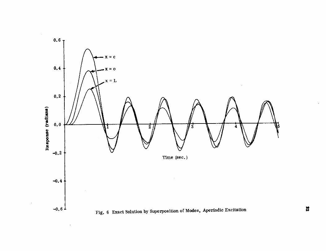
Results:

Double precision arithmetic was used for all calculations. The upper

infinite limit was replaced by forty. Thus, the exact (analytical) solution was

obtained by superpositioning of the first forty modes. Figs. 5 and 6 show the

response of sections x == 0, x == c, and x = L for the cases of periodic and

aperiodic excitation, respectively. The corresponding tabulated values can be

found from Tables VTI and Vm, respectively.

To check the accuracy of these results,asolution using the first thirty

modes was obtained. Solutions using the first forty and the first thirty modes,

' ~

... ,~'\ o.sl ·~·

1\.- x=c

0.4l ~~X=O x=L

0.2

lo.oi/U \t /2 l\ ~ \~ I ! -o.2

Time (sec.)

-o.4

-o.6 Fig. 5 Exact Solution by Superposition of Modes, Periodic Excitation

~ ...

0.6

0.4

0.2

-• § ~ e o.o G) ., s= 8. Ill

! -o.2 .

Time (sec.)

-o.4

-0.6 Fig. 6 Exact Solution by Superposition of Modes, Aperiodic Excitation =

23

for the case of periodic excitation are given in Table V. The high degree of

accuracy of the results with the first forty modes is obvious. It also justifies

the use of this solution as a basis of comparison of the approximate solutions to

be obtained in the subsequent chapters.

24

TABLE V

COMPARISON OF SHAFT I~ISPLACEMENTS

(PERIODIC EXCITATION) -SUPERPOSITION OF MODES+

Time X == 0. 0 X == 6. 0 X= 16.0

40 modes 30 modes 40 modes 30 modes 40 modes 30 modes

0.0 0.0 0.0 o.o 0.0 o.o o.o

0.2 0.04748 0.04748 0.13647 0.13607 o. 01100 0. 01100 0.4 0.28414 0.28414 0.42191 0.42126 0.14142 0.14142 0.6 o. 37800 0.37800 o. 52769 0.52705 0.25322 0.25322 0.8 0.18312 0.18312 0.25976 0.25936 0.09331 0.09331 1.0 0.11357 0.11357 0.11481 0.11481 0.09044 0.09044

1.2 -0.18762 -<>.18762 -0.26299 -0.26259 -0.09385 -0.09383 1.4 -0.14793 -0.14792 -0.29398 -0.29334 -0.07490 -0.07490 1.6 -0.27553 -0.27553 -0.41736 -0.41672 -0.13564 -0.13564 1.8 -0.27763 -0.27763 -0.37245 -0.37205 -0.18818 -0.18818 2.0 -0.01114 -0.01114 -0.00545 -0.00545 -0.01243 -0.01243

2.2 0.27229 o. 27229 o. 37379 o. 37339 0.19099 0.19099 2.4 0.30405 0.30405 0.42866 0.42802 0.15507 0.15507 2.6 0.15356 0.15356 0.28842 0.28778 0.07458 0.07458 2.8 0. 15572 0.15572 0.25152 0. 25112 0.07748 0.07748 3.0 0.11321 0.11321 0.12529 0.12529 0.08408 0.08408

3.2 -0.15909 -0.15909 -0.25251 -0.25211 -0.07124 -0.07124 3.4 -0.37091 -0.37091 -0.53432 -0.53367 -0.25009 -0.25009 3.6 -0.30822 -0.30822 -0.43174 -0.43110 -0.16176 -0.16176 3.8 -0.05870 -0.05870 -0.13222 -0.13183 -0.01239 -0.01239 4.0 0.02920 0.02920 0.01836 0.01836 0.01430 0.01430

4.2 0.05206 0.05205 o. 12720 0.12670 0.01946 0.01946 4.4 0.26247 0.26246 0.40148 0.40083 0.12310 0.12310 4.6 0.37091 0.37091 o. 53836 o. 53772 0.24510 0.24510 4.8 0.19889 0.19889 0.28224 0.28185 0.11414 0.11414 5.0 -0.09799 -0.09799 -0.12610 -0.12610 -0.08837 -0.08837

+Units of time and displacement are second and radian, respectively.

,CHAPTER W

FINITE-DIFFERENCE SOL UTI ON

Numerical finite-difference methods have been in use for a long time.

But, in recent years, due to the development of high-speed digital computers,

they have become more popular. The accuracy and computational efficiency of

these methods should be evident from the results of our one-dimensional

problem. Theoretically, two- and three-dimensional problems could be treated

in an analogous fashion although, in practice, the three-dimensional case

presents a formidable problem even for present-day large-scale computers.

A. Basic Approach:

A space and time mesh is established with mesh sizes ~ and At,

respectively. 'rhe derivatives are approximated by differences. Thus, the

differential equation is approximated by a difference equation.

Following the notations of Smith [ 7], r .. is used to denote the response. lJ

The first subscript refers to the variable x and the second to the variable t.

i = 1 refers to x = 0 and j = 1 refers to t = 0. Thus, r .. denotes the response lJ

of the ith node from the left end of the shaft after j-1 number of time increments.

Subscripts of c and L are used to denote the sections at x = c and x = L, respec-

tively.

The method can be applied to the problem directly with the non-homogeneous

Eq. (1.1). However, in order to simplify the analysis, the non-homogeneous

Eq. (1.1) is rewritten in terms of the homogeneous equation

GJ rxx =I rtt

and the jump condition

(3.1)

26

(3.2)

with the continuity requirement

- + r(c, t) = r(c , t) = r(c, t). (3. 3)

+ c-is the section of the shaft just to the left of c and c is the section just to the

right of c. The left hand side of Eq. (3.2) thus represents the shaft internal

torque at the section x =c.

Difference Formulas:

The finite-difference formulas [7], [8], [9] used in this chapter are all

of second order and are listed below for reference.

Central-difference formulas for second-order derivatives:

r. 1 . - 2r .. + r. 1 . 1+ ,] y 1- ,J

(rij)xx = i)lx..)2

r .. 1 -2r .. +r .. 1 - 1,]+ 1] 1,]-

(r .. )tt- 2 1J (At)

Forward-difference formula for first order derivative:

-r. 2 . + 4r. 1 . - 3r .. ) - 1+ .J 1+ • ] 1,]

(rij x- 2Ax

Backward-difference formula for first order derivative:

3r .. - 4r. 1 . + r. 2 . - 1] 1-,] 1-,J

(r .. ) - 2A .... 1J X IJoh

From the last two formulas:

-r3 . + 4r2 . - 3r1. - ] ] ] (r1j)x- 2Ax

(3. 4)

(3. 5)

(3. 6)

(3. 7)

(3. 6a)

3 r -. - 4r - . + r - . ( ) - _£1 c -1. ] c -2. J r- -

C j X 2_Ax

(r +.) = C J X

-r + + 4r + - 3r + c +2, j c +1' i c j

2Ax

3rL. -4rL 1. +rL 2. - J - .J - ,]

(rLj)x- 2Ax

B. The Finite-Difference Problem:

1. Associated Difference Equation:

27

(3. 7a)

(3. 6b)

(3. 7b)

Using the finite-difference formulas of the previous section, the given

boundary-value problem is reduced to the simpler problem of solving the

associated difference equation with corresponding boundary conditions.

Substitution of formulas (3.4) and (3. 5) in Eq. (3.1) yields the associated difference

equation from which, solving for r .. 1 , we obtain: 1, ]+

2 2 r. . +1 = 2 (1 - X ) r .. + X (r. +1 . + r. 1 . ) - r. . 1 , 1,] 1] 1 ,] 1- ,] 1,]-

,2 = GJ(At)2 2 At 2 1\ - 2- = a (Ax) •

I(Ax)

(3. 8)

The accuracy of the solution depends on the value of A. For A> 1, the solution

is unstable. For A :!!;; 1, the solution is stable and the accuracy increases as A

* approaches the value 1. For A= 1, the solution is "exact" except for the round-

off. In fact, if Ax= aAt, then any solution of the differential Eq. (3.1) satisfies

** the associated difference equation and conversely, regardless of mesh size [8] •

* For proof of convergence and stability, see Smith [7].

** See the results of Table VI.

28

Letting .O.x = a,At, Eq. (3.8) reduces to,

r .. l=r.l.+r.1.-r. "1" 1,J+ 1+ ,J 1- ,J 1,J-(3. 9)

2. Boundary Conditions and Jump Condition:

With formula (3.6a), from boundary condition (2.2), we get, forx = 0:

ri, j+1 = -P 1 r3j + 4P 1r2j - P 2r1j - r1, j-1'

p = GJ(At)2

1 2AxiL '

(3 .10)

Similarly, with formulas (3. 7a) and (3. 6b) from the jump condition (3. 2), for

x = c, we obtain:

2 1 r . = P3m. + 3- (r 1 . + r +1 . ) - -6 (r 2 . + r -'-'2 . ) ' CJ J c- , J c , J c- , J c-,-, , J

m. = m(t) evaluated at t = (j-1)4t, J

(3 .11)

and for x = L, from boundary condition (2. 3), with formula (3. 7b), we get:

(3.12)

The given boundary value problem is thus reformulated in terms of the

29

difference equations (3.9) to (3.12).

c. Solution of the Difference Problem:

From Eq. (3. 9) it can be seen that, to generate the solution corresponding

to time j+1, we require the values of r in the previous two rows j and j-1.

Therefore, to start the solution, we need the two starting rows corresponding to

j=1 (t = 0) and j=2 (t =At). From the initial conditions (2. 4), we have:

ril=o, for all i and

ri2=o, i~c, since, the excitation is applied at the section x = c only. The

value of rc2 can be calculated from Eq. (3.11). In fact, since for j=2, rc2 is the

only non-zero quantity,

The first two rows being known, the third row can be generated, using Eq. (3.10)

for i=2, 3, .•• , L-1. The boundary values at i=1 and i=L are then obtained

from the formulas (3.10) and (3.12), respectively.

1. Periodic Excitation:

The periodic excitation is applied at the section x =c. The response at

this section can be obtained by using the formula (3. 11). Thus, for the case of

the periodic excitation, the value of r . must be recalculated at all the time CJ

increments j.

2. Aperiodic Excitation:

As the excitation is non-zero for time t =' t only, recalculation of r . is p CJ

required only for those values of j that correspond tot :s: t • Fort> t , this p p

recalculation is not required, since the excitation fort> t is zero. The p

30

response at t = t forms an initial value problem fort >t . The values of r p p ij

corresponding to j = t and j = t - At are used to obtain the free response for p p

timet >t . p

Results:

In Table VI, the response at x = c, obtained by using different mesh sizes,

is given for the case of periodic excitation. The last row gives the computer

time in seconds. Note that the computing time for a given mesh size is

approximately the same for the case of single precision (seven significant

digits) and double precision (fourteen significant digits) arithmetic but, the

results are far more accurate for the latter case. The accuracy increases as

the grid is made finer. However, the computer time increases at a faster rate.

The results for the case of periodic and aperiodic excitation obtained by

using ~t = o. 005 are given in Tables VII and vm, respectively. Since the

response for both cases is identical for t 5: t , the results for the aperiodic p

case fort 5: t are not tabulated. These results were obtained with~= aA t. p

Time

0.0

·o.1 0.2 0.3 0.4 0.5

0.6 0.7 0.8 0.9 1.0

1.1 1.2 1.3 1.4 1.5

1.6 1.7 1.8 1.9 2.0

2.1 2.2 2.3 2.4

.2. 5

TABLE VI

EFFECT OF GRID SIZE AND PRECISION ON THE ACCURACY

Exact

0.0

0. 03829 0.13647 0. 26232 0.42191 0.52568

0.52769 0.44957 0.25976 0.05442

-0.11481

-0.24154 -0.26299 -0.26700 -0.29398 -0.33464

-0.41736 -0.43909 -0.37245 -0.23199 -0.00545

0.20769 0.37379 0.45800 0.42866 0. 36662

+ OF F-DIFFERENCE SOLUTION

F- Diff.

:At=0.001 at=o. oo1* at=o. oo5

0.0 0.0 0.0

0.03895 0.03895 0.03899 0.13772 0.13765 0.13771 0. 26403 0.26379 0.26399 0. 42392 0.42286 0.42393 0.52779 0.52513 0.52767

0. 52971 0.52521 0. 52974 0. 45128 0.44602 0.45131 0.26100 0.25631 0.26095 0.05508 0.05266 0.05525

-0.11481 -0.11328 -0.11495

-0.24219 -0.23691 -0.24227 -0.26423 -0.25698 -0.26414 -0.26872 -0.26289 -0.26876 -0.29598 -0.29425 -0.29583 -0.33676 -0.33939 -0.33704

-0.41938 -0.42399 -0.41919 -0.44078 -0.44324 -0.44017 -0.37370 -0.37142 -0.37426 -0.23264 -0.22568 -0.23265 -0.00544 0.00313 -0.00532

0.20832 0.21366 0.20783 0.37505 0.37332 0.37555 0.45971 0.45032 0.45963 0.43067 0.41766 0.43061 0.36876 0. 35828 0:36919

-At=O. 01

0.0

0.03914 0.13767 0. 26378 0.42397 0. 52749

0.52992 0.45121 0. 26074 0.05585

-0.11554

-0.24243 -0.26377 -0.26917 -0.29528 -0.33764

-0.41849 -0.43878 -0.37631 -0.23142 -0.00465

0.20500 0.37728 0. 45981 0.42968 0.37056

* with seven significant figures

+Units of time and displacement are second and radian, respectively.

31

32

TABLE VI (continued)

F- Diff. Time Exact

At=o. oo1 At==O. 001* At==O. 005 At==0.01

2.6 0. 28842 0.29041 0. 28791 0.28970 0.28857 2.7 0.24570 0.24742 0.25390 0.24774 0.24849 2.8 0.25152 0.25277 o. 26344 0.25308 0. 25282 2.9 0.20966 0.21029 0.21787 0.20941 0.20817 3.0 0.12529 0.12529 0.12437 0.12524 0.12654

3.1 -0.03484 -0.03549 -0.04493 -0.03533 -0.03665 3.2 -0.25251 -0.25374 -0.26618 -0.25308 -0.25229 3.3 -0.41759 -0.41929 -0.42684 -0.41923 -0.41878 3.4 -0. 53432 -0.53634 -0.53328 -0.53681 -0.53756 3.5 -0.54209 -0.54419 -0.53034 -0.54361 -0.54180

3.6 -0.43174 -0.43378 -0.41553 -0.43446 -0.43762 3.7 -0.29416 -0.29588 -0.28182 -0.29612 -0.29510 3.8 -0.13222 -0.13344 -0.13115 -0.13282 -0.13039 3.9 -0.02347 -0.02414 -0.03562 -0.02469 -0.02862 4.0 0.01836 0.01839 -0.02009 0.01905 0.02237

4.1 0. 06783 0.06848 0.05425 0.06842 0.06865 4.2 0.12710 0.12833 0.12620 0.12806 0.12518 4.3 0.25062 0.25239 0.26373 0.25368 0.25767 4.4 0.40148 0.40345 0.41970 0.40207 0.39956 4.5 0.50052 0.50261 0. 51382 0.50204 0.50093

4.6 0.53836 0.54040 0.53834 0.54160 0.54357 4.7 0. 45205 0.45375 0.43767 0. 45285 0.45067 4.8 0. 28224 0.28353 o. 26212 0.28396 o. 28636 4.9 0.08214 0. 08281 0. 06587 0.08323 0. 08343 5.0 -0.12610 -0.12613 -0.12792 -0.12637 -0.12704

208** 185 28 21.3

**Computer time in seconds.

33

TABLE VII

F-DIFFERENCE SOLUTION, PERIODIC EXCITATION, At= 0.005+

X= 0 ~ = c X,= L Time

Exact F-Diff. Exact F-Diff. Exact F-Diff.

0.0 0.0 0.0 0.0 0.0 o.o 0.0

0.1 o. 00151 o. 00149 0. 03829 0.03899 0.00000 -0.00000 0.2 0.04748 0.04750 0.13647 0.13771 0.01100 0.01099 0.3 0.16529 0.16531 0.26232 0.26399 0.06364 0.06363 0.4 0.28414 0.28406 o. 42191 0.42393 0.14142 0.14140

0.5 0.36471 0.36471 0. 52568 0.52767 0.22002 0.22006

0.6 o. 37800 0.37798 o. 52769 0.52974 0.25322 0.25321

0.7 0. 30241 o. 30241 0.44957 0.45131 0.19935 0.19934

0.8 0.18312 0.18324 0.25976 0.26095 o. 09331 o. 09335

0.9 0.02814 0.02810 o. 05442 0. 05525 -0.01894 -0.01898

1.0 -0.11357 -0.11357 -0.11481 -0.11495 -0.09044 -0.09036

1.1 -0.17877 -0.17882 -o.24154 -0.24227 -o.10325 -o.10324

1.2 -0.18762 -0.18769 -o.26299 -0.26414 -0.09383 -0.09398

1.3 -0.15502 -0.15488 -0.26700 -0.26876 -0.07761 -0.07761

1.4 -0.14793 -0.14805 -0.29398 -0.29583 -0.07490 -0.07494

1.5 -0.20820 -0.20820 -0.33464 -0.33704 -0.09896 -0.09886

1.6 -0.27553 -0.27542 -0.41736 -0.41919 -0.13564 -0.13548

1,7 -0.31505 -0.31509 -0.43909 -0.44017 -0.18042 -0.18055

1.8 -0.27763 -0.27735 -0.37245 -0.37426 -0.18818 -0.18819

1.9 -0.15770 -0.15787 -0.23199 -0.23265 -0.12513 -o.12516

2.0 -0.01114 -0.01139 -0.00545 -0.00532 -0.01243 -0.01246

2.1 0.14952 0.14966 0.20769 0.20783 0.11549 0.11556

2.2 0.27229 0. 27205 o. 37379 0.37555 0.19099 0.19084

2.3 0.32189 0.32215 0.45800 0.45963 0.19220 0.19221

2.4 0.30405 0.30427 o. 42866 0.43061 0.15507 0.15515

2.5 0.22125 0. 22091 0.36662 o. 36919 0.10340 0.10348

+Units of time and displacement are second and radian, respectively.

34

TABLE VII (continued)

x •o X.= C X =L Time

Exact F-Diff. Exact F-Diff. Exact F-Diff.

2.6 0.15356 0.15373 0.28842 0.28970 0.07458 0.07480

2.7 0.13952 0.13943 0.24570 0.24774 o. 07158 0.07131

2.8 0.15572 0.15568 0. 25152 O.Z5308 0.07748 o. 07729

2.9 0.17281 0.17292 0.20966 0.20941 o. 09368 o. 09373

3.0 0.11321 0.11277 0.12529 0.12524 0.08408 0.08401

3.1 -0. 01415 -0.01399 -0.03484 -0.03533 0.02754 0.02783

3.2 -0.15909 -0.15887 -0.25251 -0.25308 -0.07124 -0~ 07127

3.3 -0.29925 -0.29914 -o. 41759 -0.41923 -0.18724 -0.18741

3.4 -0.37091 -0.37064 -0.53432 -0.53681 -0.25009 -0.24983

3.5 -o. 37234 -o. 37284 -o. 54209 -0.54361 -0.23504 -o.23517

3.6 -0.30822 -o.30828 -0.43174 -0.43446 -0.16176 -0.16175

3.7 -0.17700 -0.17700 -0.29416 -0.29612 -0.06916 -0.06920

3.8 -0.05870 -o.05881 -o.13222 -o.13282 -0.01239 -0.01279

3.9 0.01294 o. 01355 -o. 02347 -0.02469 o. 01120 0. 01143

4.0 o. 02920 0.02880 01 01Er3:'6 0.01905 0. 01430 0.01456

4.1 o. 01365 o. 01358 0.06783 0.06842 0.00630 0.00648

4.2 0.05206 o. 05264 0.12710 0.12806 0.01946 0.01953

4.3 0~ 14495 0.14455 04 25062 0.25368 0.05547 0.05502

4.4 0. 26247 o. 26267 o. 40148 0.40207 0.12310 0.12312

4.5 0.35880 0.35845 0.50052 0.50204 0.20727 0.20731

4.6 0. 37091 0.37034 o. 53836 0.54160 o. 24510 0.24508

4.7 0.31682 o. 31761 o. 45205 0.45285 0.21376 0.21395

4.8 0.19889 0.19892 o. 28224 0.28396 0.11414 0.11387

4.9 0. 03925 o. 03945 0.08214 0.08323 -o. 00932 -0.00909

5.0 -0.09799 -0.09783 -0.12610 -0.12637 -0.08837 -0.08809

35

TABLE VIII

F-DIFFERENCE SOLUTION, APERIODIC EXCITATION, At= 0. 005 +

x=O X. = c x=L Time

Exact F-Diff. Exact F-Diff. Exact F-Diff.

1.1 -0.17726 -0.17739 -0.20324 -0.20334 -0.10325 -o.10324 1.2 -0.14014 -0.14030 -0.12652 -0.12655 -0.08283 -0.08305 1.3 0.01027 0.01041 -0.00468 -0.00488 -0.01397 -0.01402 1.4 0.13622 0.13603 0.12792 0.12820 0.06651 0.06644 1.5 0.15651 0.15654 0.19104 0.19074 0.12106 0.12122

1.6 0.10246 0.10264 0.11033 0.11049 0.11758 0.11782 1.7 -0.01264 -o. 01264 o. 01048 0.01121 0.01893 0.01885 1.8 -0. 09452 -0.09408 -0.11269 -0.11327 -0.09487 -0.09485 1.9 -0.12957 -0.12979 -0.17757 -0.17745 -0.14408 -0.14418 2.0 -0.12471 -0.12508 -0.12025 -0.12019 -0.10287 -0.10289

2.1 -0.02925 -0.02922 -0.03384 -0.03457 0.01224 o. 01230 2.2 0.08466 0.08436 0.11080 0.11124 o. 09715 0.09687 2.3 0.16687 0.16729 0.19100 0.19093 0.11459 0.11462 2.4 0.15613 0.15635 0.13468 0.13496 o. 08016 0. 08027 2.5 0.01305 0. 01277 o. 03198 0.03240 0.00444 0.00465

2.6 -0.12197 -0.12169 -0.12894 -0.12966 -0.06105 -0.06066 2.7 -0.17553 -0.17569 -0.19339 -0.19277 -0.10885 -0.10922

2.8 -0.12191 -0.12180 -0.12093 -0.12109 -0.11070 -0.11099

2.9 o. 01511 0. 01503 -0.02232 -0.02307 -0.03146 -0.03151

3.0 0.10207 0.10136 0.11984 0.11996 o. 07165 o. 07153

3.1 0.13537 0.13564 0.17285 0.17235 0.14303 0.14344

3.2 0.11320 0.11332 0.12128 0.12232 0.11974 0.11966

3.3 0.02264 0.02308 0.04041 0.04069 0.00496 0.00482

3.4 -0.06686 -0.06636 -0.10565 -0.10618 -0.09502 -0.09469

3.5 -0.15110 -0.15193 -0.17546 -0.17465 -0.13164 -0.13170

+Units of time and displacement are second and radian, respectively.

36

TABLE VITI(continued)

X= 0 X= C X=L

Time Exact F-Diff. Exact F-Diff. Exact F-Diff.

3.6 -0.15465 -0.15467 -0.14332 -0.14459 -0.08718 -0.08703

3.7 -0.03749 -o. 03762 -0.04846 -0.04857 0.00242 0. 00210

3.8 o. 09702 0.09682 0.11929 0.12003 o. 06510 0.06448

3.9 0.18575 0.18646 0.18619 0.18515 0.10487 0.10514

4.0 0.14241 0.14175 0.14365 0.14465 0. 09838 0.09864

4.1 -0.00050 -9~00037 0. 03299 0.03290 0.03384 o. 03437

4.2 -0.10703 -0.10623 -0.12541 -0.12555 -0.05178 -0.05168

4.3 -0.15430 -0.15456 -0.16696 -0.16540 -0.13177 -0.13242

4.4 -0.10844 -0.10808 -0.13283 -0.13435 -0.12699 -0.12687

4.5 -0.01354 -0.01444 -0.04156 -0.04201 -0.02777 -0.02788

4.6 o. 06269 o. 06198 0.10662 0.10688 o. 08333 0.08333

4.7 0.13982 0.14063 0.15790 0.15707 0.14460 0.14476

4.8 0.14019 0.14025 0.15002 0.15145 0.10175 0.10118

4.9 0. 05219 0. 05298 o. 05867 0.05868 0.00187 o. 00236

5.0 -0.06879 -0.06892 -0.10774 -0.10755 -0.07407 -0.07350

37

CHAPTER IV

FOURIER TRANSFORM SOLUTION

A. Introduction:

In recent years, due to the development of high-speed digital computers,

the Fourier transform method is being used as a powerful mathematical tool. The

numerical application of this method plays a crucial role in a stochastic approach

to the dynamic structural analysis, [10], [11]. In the field of spectroscopy, a

substantial amount of work.has been done in recent years, using Fourier trans-

* form as a convenient tool [12].

There exists a direct analogy between the analysis of system response

by Fourier series methods for periodic excitation and the Fourier transform

method for aperiodic excitation. In the following analysis, the numerical

application of the Fourier transform method is examined for the case of

aperiodic excitation.

1. Fourier Transform Pair Definition:

Fourier [13] extended the Fourier series representation into Fourier's

integral formula

•• 1 f(x) = -J[ Jf(t) cos y(x - t) dt]dy.

"o -=

Although several alternate forms of this formula are possible, the most

commonly accepted form proposed by Cauchy is the exponential form:

*It has been pointed out that under certain conditions, the induction decay signal obtained in a pulsed nmr experiment and the cw-nmr spectrum constitute a Fourier transform pair.

38

CCI CD

f(x) =z;sc J f(t) e -iwtdt] eiwxdw. -co -CD

The direct Fourier transform and the inverse Fourier transform are

defined by Eqs. (4.1) and (4. 2), respectively.

011

'F [f(t~ = F(w) = J f(t) e -iwtdt (4.1) -co

CCI

'F" -1[F(w)] = f(t) = ~ JF<w> eiwtdw. -41

(4. 2)

Eqs. (4.1) and (4. 2) form a transform pair which permits a trans forma-

tion of the variable t into a function of the new variable w, thus replacing the

problem posed in the time domain by a problem posed in the frequency domain;

often leading to a simplification. For F(w) to exist, the function f(t) must satisfy

the following Dirichlet conditions [14]:

(1) f(t) has, at most, a finite number of discontinuities.

(2) f(t) has, at most, a finite number of maxima and minima. 011

(3) The integral Jl f(t) I dt is finite. -CXI

However, this question of the existence of the Fourier transform seldom arises

for most of the practical transient vibration problems.

2. Basic Approach:

The application of the Fourier transform method requires the following

three steps:

(1) Obtain the system transfer function H(w).

The system transfer function is a complete description of the system

39

* and it predicts the system response for any type of excitation. It is

usually a complex function of the real variable w.

(2) Obtain the excitation transform M(w).

This is also usually a complex function of w. If the excitation is of

simple form, describable analytically, the transform can be determined

exactly using the definition (4.1); otherwise, M(w) has to be computed

numerically using the (approximate) numerical quadrature methods based

on the Newton-Cotes type formulas. For derivation and discussion of

these methods see Ref. [ 1].

(3) Form the response transform,

R(W) = H(W)M(W) (4.3)

and perform the inversion integration (4. 2) to obtain r(t).

The response transform can be inverted either analytically using

formula (4. 2) or, in the case of complicated analytical integrations,

numerically as stated in the previous step. Although the above

expression for R(w) is "exact" for the problem considered here, it

should be pointed out that, for non-zero initial conditions an extra term

must be added to the right hand side, as shown by Aseltine [15].

Some Results:

For the case of aperiodic excitation (applied at timet= 0), the response

r(t) is non-zero only for a finite length of time. Therefore,

* . . input Transfer function usually sign.1fies tp t' see Eq. (4. 3). ou u

r(t) = dr(t) = o dt

at t = ± 1:10.

Hence, after integrating by parts, we get:

.. J dR(W) e -iwtdt = :iw R(w)

,, dt --.. 2 J d R(W) e -iwtdt = -w2R(w),

-co dt2

40

(4. 4)

(4. 5)

(4. 6)

where R(w) is the direct Fourier transform of r(t), defined in Eq. (4.1).

To find the response r(t), we have to invert the response transform R(w).

Substituting Eq. (4. 3) in terms of real and imaginary components, into the

inverse formula (4. 2), we obtain:

011

r(t) = ..!.. J [Re R(w) cos wt - ImR(w) sin wt] dw

211.-

.. i J +- (ImR(W) cos wt + ReR(W) sin wt]dw.

2'1r- . (4. 7)

As shown by Barker [l.J, for real r(t), this expression reduces to:

.. r(t) =;. J[ReH(w)ReM(w)- ImH(w) lmM(w)] cos wt dw

·o

co

- ~ J [Re H(w) ImM(w) + ImH(w) Re M(w)] sin wt dw.

0

(4. 8)

If there is no damping in the system, H(w) is real and Eq. (4. 8) further

reduces to

co

r(t) = ; J [Re R(W) COB wt - I mR(W) Bin wt] dw. (4. 9)

'0

.41

B. Response Transform:

1. Reformulation of the Problem:

Since m(t) is a concentrated torque acting at the location x = c, the

system can be analyzed by cutting the shaft at the applied torque. As in the

previous chapter, the non-homogeneous Eq. (2.1) is decomposed into the

homogeneous Eq. (3.1) and the jump condition (3. 2), with the continuity

requirement (3. 3). For this case, the jump condition is further decomposed

into

GJ r (c, t) = m.(t) X 1

(4.10)

+ GJ r (c ,t) = m.(t)- m(t), X 1

(4.11)

m. (t) being the shaft internal torque at x =c. Thus, the boundary conditions 1

for the region 0 ~x ~ c become:

(4. 12)

GJ r (c- , t) = m (t) X i

(4.10)

+ and for the region c ~:X~ L, they are:

+ GJ r (c ,t) = m.(t)- m(t) X 1

(4.11)

(4. 13)

Using the definition (4.1) and the results (4. 5) and (4. 6), the problem

in the time domain is now transformed into a problem in the frequency

domain. The transformed equation of motion is,

2 d R~,w) +()!.~ R(x,w) = 0,

dx

(4.14)

w a=-. a

The solution to this equation is given by:

R(x, W) = A(W) sin~ + B(W) cos QX

42

(4.15)

where, the arbitrary functions A and B of w are to be obtained from the boundary

conditions.

Let us first consider the solution for the region 0 :s;: x s c.

Boundary conditions (4.12) and (4.10) on transformation, become:

dR(O, W) = _, R(O ) dx ""L ' W

dR(c; w> = M_i<_w_> dx GJ

From these and from Eq. (4.15) we obtain:

~L A=-- B,

«

Mi(W) B = - ----=:...-------

GJ(~L cos a c + 01 sin a c)

so that for 0 s x s c,

Mi (W) O..L sin ax - a cos ax) R(x, W)= GJ( XL cos ac +o: sin a c)

(4.16)

(4.17)

(4.18)

In a similar way, for the region c s x s L, from the transformed boundary

conditions

dR(o +. w> = Mi (w) - M(w)

dx GJ (4.19)

43

dR(L, w) dx = AR R(L, w), (4.20)

we obtain:

- . 1 . + . 1 (M. (W) - M(W) 1 A - cos a c ', ~ GJ B sm ~c '

Mi~) - M(w) (ct cos aL - AR sincr L ~

B = aGJ(>..R cosa(L-c) +a sina(L-c)J

so that, for this region,

Mi(w) - M(w) a cos a (L- x) - XR sin a (L- x)

R(x, W) = aGJ 'An cos «X (L -c) +ex sin~ (L - c) (4.21)

The unknown M.(W) can be determined by requiring Eqs. (4.18) and (4.21) 1

to agree on the expression for the response transform at x =c. Thus,

(a sin ac +XL cos ac)li:x cos a (L -c) - XR sin a (L -c)] Mi(W) = 2 M(W)

C¥~L + XR) cos Let + (01 - XRXL) sin Let

2. System Transfer Function:

Substituting for M.(W) in Eq. (4.18) and dividing by M(w) yields the 1

transfer function for the portion of the shaft between x = 0 and x =c. Calling

this expression HL (x, w), we get:

[0! cos ex (L-c) - XR sin a (L-c) ]~L sin ax-a cos ocx) W) = •

QGJfc¥~L + XR) cos l..tlt + (r:l -XL AR) sin Loc]

A similar substitution of M.(W) into Eq. (4.21) yields the transfer 1

(4.22)

44

function for the remainder of the shaft in the region c s; x s: L. Denoting this

transfer function by HR (x, W), we obtain:

(a cos 01 c - >..L sin oc c){XRsin (L-x)cx -a cos (L-x) a] W) = 2 •

~J~~L + >..R) cos La + tt - )..L )..R) sin La] (4. 23)

From these expressions, the transfer function for any location x of the

shaft can be obtained.

3. Excitation Transform:

After the system transfer function has been found, the next step in

applying the Fourier transform method to a specific problem is to determine the

excitation transform.

For the excitation given by Eq. (1. 6), from the definition (4.1), we

obtain:

t P -iwt

Mt.J) = J M sin wet e dt 0

-iwt t = _ Me (iw sin w t - w cos w t) I P

2 2 e e e 0 we -w

= Mw

e (e -iwtp + 1 ).

2 2 w -w e

Hence,

MWe Re M(W) = --2----2~ (cos wtp + 1),

w -w e

(4.24)

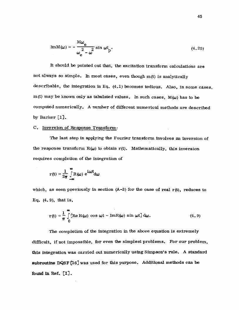
45

Mwe ImM(w) = - 2 2 sin wt .

w -w P e

(4. 25)

It should be pointed out that, the excitation transform calculations are

not always so simple. In most cases, even though m(t) is analytically

describable, the integration in Eq. (4.1) becomes tedious. Also, in some cases,

m(t) may be known only as tabulated values. In such cases, M(W) bas to be

computed numerically. A number of different numerical methods are described

by Barker [1].

C. Inversion of Response Transform:

The last step in applying the Fourier transform involves an inversion of

the response transform R(W) to obtain r(t). Mathematically, this inversion

requires completion of the integration of

1 • iwt r(t) = 2 JR(W) e dw " ..

which, as seen previously in section (A-3) for the case of real r(t), reduces to

Eq. (4. 9), that is,

CID

r(t) = !. J (Re R(w) cos wt - ImR(w) sin wt] dw. 1T 0

(4. 9)

The completion of the integration in the above equation is extremely

difficult, if not impossible, for even the simplest problems. For our problem,

this integration was carried out numerically using Simpson's rule. A standard

subroutine DQSF 1:16] was used for this purpose. Additional methods can be

found in Ref. (IJ.

46

The added complication due to the infinite upper limit on the range of

integration is not a very serious problem since, for most cases, the integration

converges for a sufficiently large value of a,t.,(denoted by w ) . However, the max

choice of wmax plays a very impo~tant role as far as the accuracy of the results

is concerned and requires careful consideration.

The inversion formula (4. 9) can now be rewritten as:

1 r(t) = ,

Wmax

J 0

[ Re R(w) cos wt- ImR(w) sin w t] dw. (4. 26)

The integration step size H is equally important. A smaller step size

gives a more accurate solution but requires more computer time. In the results

given in Table JX, computer times required for the step sizes of H = 0. 5,

H = o. 25, and H = 0.1 with w = 100 were 32 seconds, 45 seconds and 87 max

seconds, respectively. However, these results show no definite pattern,

contrary to the fact that the accuracy should increase as the step size is made

smaller.

The explanation for this indefinite pattern lies in the behavior of the

system transfer function H(x, w ).. The denominator of the system transfer

function is dependent only on the system constants and thus, is a characteristic

of the given system [see Eqs. (4.22) and (4.23)] • The zeroes of this

characteristic function were calculated and it was observed that these zeroes

correspond to the natural frequencies of the system. The first four zeroes

(poles of the system transfer function) of the denomipator in the system transfer

function are:

TABLE IX

SHAFT DISPLACEMENTS AT x = 6. 0 -- F-TRANSFORM SOLUTION+

"'max= 200 Wma.x = 100

Time Exact H =0.1 H =0.1 H = 0. 25

0.0 0.0 -0.22210 -0.22179 -0.16994

0.1 o. 03829 -0.21326 -0.21300 -0.10312 0.2 0.13647 o. 02691 o. 02695 o. 08113 0.3 0.26232 0.35320 0.35309 0.34623 0.4 0.42191 o. 64264 0.64251 0.57940 0.5 0.52568 0.79208 o. 79194 0.67463

0.6 0.52769 0. 64264 0.64251 o. 57940 0.7 0.44957 0.35321 0.35309 0.34624 0.8 0.25976 o. 02691 o. 02695 0. 08113 0.9 0. 05442 -0.21326 -0.21300 -0.10212 1.0 -0.11481 -0.22210 -0.22179 -0.16194

1.1 -0.20324 -0.11246 -0.11229 -0.10768 1.2 -0.12652 o. 09298 0. 09283 0. 02371 1.3 -0.00468 0.24811 0.24775 0.12791 1.4 0.12792 0.23322 o. 23296 0.17015 1.5 0.19104 0.11666 0.11662 0.10459

+ Units of time and displacement are second and radian, respectively.

H = 0.5

-0.03644

o. 05435 0.15140 0. 31198 0.48104 0. 54617

!

0.48104 0.31198 1

0.15140 0.05435

-0.03644

-0.09682 -0.10550 -0.05895 0.06650 0.11701

~ -:J

Time Exact

1.6 0.11033 1.7 0. 01048 1.8 -0.11269 1.9 -0.17757 2.0 -0.12025

2.1 -0.03384 2.2 0.11080 2.3 0.19100 2.4 0.13468 2.5 0.03198

TABLE IX (continued)

Wmax = 200

H =0.1 H =0.1

-0.10760 -0.10747 -0.25881 -0.25867 -0.22806 -0.22795 -0.11494 -0.11478 0.10603 0.10618

0.23779 0.23779 0.22375 0.22349 0.11844 0.11807

-0.09552 -0.09569 -0.23286 -0.23272

CA.max = 100

H = 0. 25

-0.04756 -0.15386 -0.18178 -0.10232

0.03756

0.12658 0.15699 0.09068

-0.03280 -0.12621

H = 0. 5

0.05743 -0.02833 -0.11211 -0.09008 -0.03460

-0.02054 0.02032 0. 04071 0.06141 0. 04794

I

~ (Xi

49

w1 = 7. 8075, w2 = 12.4706, w3 = 24.0787 and w4 = 41.6227.

As can be seen from Table IV, these are equal to the first four fre-

quencies. It was also observed that for higher values of n, the nth pole of

H (x, w) was equal to the nth natural frequency. Thus, the poles of the system

transfer function H (x, w) (as stated earlier, these depend on the system

parameters only ) correspond to different modes of oscillation.

Sufficient number of modes must be considered in order to obtain a

fairly accurate solution. Solutions for w = 100 and w = 200 with H = 0.1 max max

are shown in Table IX. Comparison of these results indicates that increasing

w from 100 to 200 has only a small effect on the solution. The value of max

w = 100 was therefore used to obtain solutions with other step sizes , H. max

Since the poles of the system transfer function correspond to the natural

frequencies of the system, in the absence of damping these frequencies result

in singularities of the integrand of the inverse Fourier integral. Therefore, this

integration cannot be performed numerically using the standard numerical

quadrature techniques.

Let the function g~l), as shown in Fig. 7, contain the singularities w= c.t•1

and w = w in the interval [ 0, w ] of the integral 2 max

wmax

T = J g~) dw. 0

This integral represents the area under the curve. To compute this area

numerically, the interval [ O,wmax] is divided into N number of equal subintervals

of step size H = w /N. Elemental areas dA. are computed using the ordinates max 1

g ( H(i + 1/2)}. The ap~roximate v8lue ofT is then obtained by summing up all the

g(w)

dA.

iH~ H 1+­nH

...----(n+l) H

Fig. 7 Example of a Non-analytic Integrand

elemental areas dAi:

N T = ~ ciA1.

i=l

50

""'max w

A typical step size H near the singularity w = w1 is shown in Fig. 7. An

ideal location of this step size requires that the net area under the curve spanned

by this step size be zero. The choice of an ideal step size obviously depends on

the function g(W). The behavior of the function g(w) is, in general, different in

the vicinity of different singularities. A step size H which is ideal across one

singularity will not, therefore, be ideal across some other singularity. No single

step size ideal for the entire interval [0, w J could therefore be obtained. A max

more sophisticated approach is required to treat ·such problems. No rigorous

51

attempt was, therefore, made to accurately compute the inverse Fourier integral

numerically.

The application of the Fourier transform method presents no such problem

in the case of damped systems as shown by Barker [1] who has used this method

in obtaining results for which the rms error was less than 1%.

52

CHAPTER V

LAPLACE TRANSFORM SOLUTION

A. Introduction:

Laplace transform method is similar to the Fourier transform method

discussed in the previous chapter. This will be obvious from the basic approach

of obtaining the response transform described in the next section.

The definition of the Laplace integral, co

F(s) = J f(t)e -st dt (5.1)

0

is, in fact, a simple modification of the Fourier integral (4.1). The function

f(t) is now defined to be zero for negative t, and the integral in Eq. (4.1) is

multiplied by a "converging factor" e-at, a > 0 so that the integrand approaches

zero fast enough to allow many integrals like

IX)

J -at -iw t f(t)e e dt ; a , w real

0

-at to converge when they do not converge in the absence of thee factor. A

simple example of such a function f(t) is the unit step function, which is common

in many practical problems [17] •

Defining the complex variable,

s =a + iw

the integral in Eq. (5.1) converges in the half plane Re(s) > k, k > 0 and the

Laplace transform is thereby defined in this region. The proof of convergence

is given by LePage [17].

53

B. Response Transform:

1. System Transfer Function

As previously stated in this chapter, the approach to obtain the response

transform is the same as that for the Fourier transform method. Taking the

Laplace transform of both sides of the governing homogeneous Eq. (3.1), we get:

d2 ao ao 2 GJ- J r(x, t)e-st dt =I J a r(x2 t) e -stdt

dx2 ot 0 0

or, denoting the Laplace transform of r(x, t), given by co

-st L[ r(x, t) ] = J r(x, t) e dt,

0

by R(x, s)

2 2 GJ d R(x, s) = I [s R(x, s) - s r(x, 0) - rt(x, 0)] •

dx2

This transformed governing equation, because of the zero inital conditions (2.4),

reduces to:

2 2 2 d R(x, s) - b s R (x, s) = 0, dx2

(5. 2)

The solution to this equation is given by:

bsx -bsx R(x, s) = Ae + Be (5.3)

From Eqs. (4.12) and (4.10), for the region 0 s: x s: c, we obtain the

transformed boundary conditions

GJ Rx(O, s) = ).L R(O, s)

GJ R (c-, s) = M. (s) , X 1

(5.4)

(5. 5)

54

and Mi(s) is the Laplace transform of the shaft internal (resistive) torque mi(t)

at x =c.

From these boundary conditions, substituting the general solution (5.3),

we obtain:

A=

B=

). = GJbs

so that for 0 ~ x ~ c,

(5. 6)

In a similar way, boundary conditions (4.11) and (4.13) are transformed

to:

+ GJ R (c , s) = M.(s)- M(s)

X 1

GJ Rx(L, s) = -). RR(L, s) ,

2 >n = JRs + KR

(5. 7)

(5. 8)

where M(s) is the Laplace transform of the excitation function m(t). From

Eqs. (5. 6), (5. 7), and {5. 8), we obtain:

(X+). )e2bsL.(M.(S)- M(S)} A= R 1

'[" L bsc bs(2L-c)J A \1\ -.R)e - (). +). R)e

55

(A -L) (M.(s) - M(s)} B= ·~ 1

A [<A -X )ebsc _ <A +X )ebs(2L-c)] R R

Hence, for the region c ::; x::; L, we get:

bs(2L-x) ·· bsx (X +~)e · · · + (X -~)e

R(x, s) = X[(A-~)ebsc _ (X +~"R)ebs(2L-c)J

[M.(s) -M(s)}. 1

(5. 9)

The unknown M. (s) can be determined, as in the case of the Fourier 1

transform method, by requiring Eqs. (5.6) and (5.9) to agree on the expression

for the response transform at x =c. Thus,

J bs(2L-c) bsc [(X-X )e -bsc -(X-X )ebsc [(X+XR)e +(X -~)e J

L L

Substituting this expression for M.(s) into Eqs. (5. 6) and (5. 9), after 1

dividing by M(s), we obtain the following expressions for the system transfer

functions HL (x, s) and ~ (x, s) for the regions 0 ::; x ::; c and c ::; x ::; L, respec­

tively:

(5.10)

H (x, s) = 2bsL R 2)[(X+X )(X+X )e - (X-L )(X-X )]

R L "R L

bsc -bsc bsx bs(2L-x) [(X+X )e +(A-X )e ][ (A-'L )e +(X +X )e ]

L L 'R L

(5.11)

2. Excitation Transform

Having determined the system transfer function H(x, s), we need the exci-

tation transform M(s) to determine the response transform

R(x, s) = H(x, s) M(s) • (5.12)

56

As discussed in Sec. E, there exist several restrictions on the nature of

the response transform R(x, s) that can be accurately inverted numerically. Only

the case of the periodic excitation will, therefore, be considered.

The Laplace transform of the sinusoidal excitation

m(t) = M sinw t e

is given by (from the table of Laplace transform pairs) :

we M M(s) = 2 2 •

s +w e

(5 .13)

Using Eqs. (5.10), (5.12), and (5.13), the response transform at any

location of the shaft can be determined. The next step is to invert this

response transform in order to obtain the response r(x, t) at a particular location.

However, let us recall that the Laplace transform in the case of a complicated or

tabulated excitation form will have to be computed numerically.

C. Inversion of Response Transform:

1. Conventional Methods

The simplest of the conventional methods is based upon the availability

of a table of Laplace transforms and inverses. As might be expected, this

approach fails, in general, for most of the complicated problems encountered

in practice. If however, F(s) is known as a function of a complex variable

over various regions of the s-plane, we can use the complex inversion formula

1 f (t) ::: 21T i

st J F(s) e ds

c

where c is a carefully chosen contour. Using the classical techniques of con-

tour shifting and residue evaluation, we can also obtain important information

57

concerning the asymptotic behavior of f(t) as t-+ oo. In a number of cases, when

we possess an explicit analytic representation of F(s), the behavior of F(s) as

s -+ 0 or s -+ =can be determined using the Tauberian theory [2]. The draw-

back to the last two approaches is that knowledge of F(s) is required in the

complex plane whereas in many applications we possess information concerning

F(s) only on the positive part of the real axis.* The best known inversion for-

mula,

f(t) =lim k -+=

(-l)k k!

k k +1 (";-) t

F(JL) t

due to Post and Widder [18] is not recommended when the derivatives are to

be computed numerically, the numerical differentiation being a very inaccurate

procedure.

With these considerations in mind, the numerical inversion technique

developed by Bellman, Kalaba and Lockett [2] was employed to obtain the

response r(x, t). ** This technique is briefly described below.

2. Numerical In version Technique

This technique is based on numerical quadrature and tre quadrature for-

mula is developed in connection with the Legendre polynomials.

a. Numerical Quadrature

The essential and completely classical idea on which this numerical

in version technique is based is that of replacing an integral by a finite sum.

*This is, of course, not true for the problem considered here.

**Several recently developed techniques to numerically invert the Laplace

transform are described in Refs. (19], (20].

58

This quite simple and reasonable approximation procedure reduces the solution

of the linear integral equation,

CCI

J -st f(t)e dt == F(s)

0

to that of the solution of a system of linear algebraic equations.

Consider an approximate expression of the type

q N

J g(x) dx =:: ~

p j==1

In order to make immediate use of classical results available for ortho-

gonal polynomials [21], let us make p = -1 and q == 1 through a suitable change

of variable;

_ p + q- 2x y- p-q

so that the above approximate relation becomes:

1 N

J g(y) dy 2! 1; W. g(y.) j=1 J J

-1

(5.14)

where w. andY. are adjustable parameters. The weighting functions w. are J J J

introduced to provide additional degrees of freedom so that as few values of

g(y) have to be evaluated as possible. To choose the parameters w. andy .• the J J

procedure inaugurated by Gauss is followed which requires that the approximation

(5.14) be "exact" for any polynomial of degree less than or equal to 2N- 1. A

detailed discussion of this procedure and the Gaussian criterian is given by

Ralston [22]. For the discussion of this procedure in connection with the

Legendre. polynomials, see Ref. [2l

59

b. Legendre Polynomials -Connection with Numerical Quadrature:

In order to satisfy the above mentioned Gaussian criterion, the poly-

nomials p n (y) of degree n must satisfy the following orthogonality conditions:

1 m J Y P n (y)dy = 0 , m = 0, 1~ ••• , n - 1

-1

1 n J Y Pn (y)dy = 1.

-1

The proof of existence and uniqueness of these polynomials is given in Refs.

[2], [22].

One family of such polynomials is that of the famous Legendre poly-

nomials*, defined by,

1 p n(Y) = n

2 nl

with the corresponding orthogonality conditions:

1

S P (y)P (y)dy = 0, m ~ n m n

-1

1 S 2 ...;2;;..,__

p (y)dy = n + 1 n

-1

It has been shown [2] that if Yj and wj in Eq. (5.14) are chosen

according to the Gaussian criterian stated in the previous subsection, then

Y J• = 1 2 N are the zeroes of PN(y) and ' ' ' ... , ' j

*For procjf, see Refs. [2], [22].

60

w = j

1 PN(y)dy s

-1 (y-y.)PN' (y.) J J

, j=1, 2, ••• , N.

Shifted Legendre Polynomials:

In order to simplify the computations, we will use quadrature formulas

over the interval [ 0, 1] • The Legendre polynomials designed for the interval

[-1,1] are, therefore, replaced by the shifted Legendre polynomials

* PN (y)=PN(1 -2y).

The resulting approximation is then:

0

1 N J g(z) dz = I;

j=1

z= 1 +y

2

w g(z.) j J

*

(5.15)

z are now the zeroes of the shifted Legendre polynomials pN· (z) and the w. are j . J

a new set of weights. Tables of these parameters are given in Appendix Two

of Ref. [2].

c. Application of Quadrature Formula

Let us start with the response transform, 00

-st R(s) = J e r(t) dt.

0

Introducing a new variable of integration

-t z=e

the above expression becomes

1 s -1 J z r(-log z) dz = B.{s) •

0

(5.16)

61

Writing g(z) = r(-log z), we may consider that we begin with the integral equation

1

f s-1 z g(z) dz = F(s) .

0

Applying the quadrature formula (5.l5), we obtain the approximate relation:

N ~

j=1 (5 .1 7)

Letting s assume N distinct values (excluding any poles of F(s)). says = it.s.

i = 1, 2, ••. , N, we obtain a linear system of N equations inN unlmowns g(z.), J

j=1, 2, ••• , N:

N i.As .

~ wJ. zJ. g(zJ.) = F (1.A s - 1), i = 1, 2, .•. , N. j=1

(5.18)

The solution of this system of linear equations yields the response r(t) at

time t = -log z., j = 1, 2, .•. , N. J

D. Solution:

Before going into the discussion of the results, let us note a few important

points. The most important of these is the question of stability. Mathematically,

the Laplace inverse is an unbounded operator. In other words, arbitrary small

changes in F(s) can produce large changes in the value of f(t). The instability

of the numerical method of the previous section manifests itself in the behavior

of the matrix [wjzj i.As]; i, j = 1, 2, ••. , N, which is ill-conditioned. The

ill-conditioning rapidly worsens as N increases [2]. The stability also depends

on the value of b,s. The solution is unstable for very small or very large values

of As, but becomes more and more stable as Af3 approaches unity. Both these

facts are illustrated through the results obtained for x = c, given in Table X.

Time N

2.1830 3 0.6931 0.1196

2.6674 4 1.1086 0.4005 0.0720

3.0595 5 1.4664 0.6931 0.2624 0.0480

3.3883 6 1.7755 0.9658 0.4791 0.1856 0.0343

+

TABLE X

+ SHAFT DISPLACE:MENTS AT x = 6. 0 ... _ L-TRANSFORM SOLUTION

~IJ Exact

0.5 1.0 1.2 1.5 2.0

0.3476 -o. 256 E-1 -o.105E 0 -0.166 E 0 -0.322E 0 -o. 976E 0 0.4583 0.102 E 0 0.214E 0 0.253E 0 0.311 E 0 0.416E 0 0.0547 0. 260 E 0 0.161 E 0 0.139E 0 0.115E 0 0. 892 E-1

0. 2529 0. 595E-2 -o.344E-1 -0.871 E-1 -o.246E 0 -o.846E 0 -0.2473 -o.l17E 0 -o. 542 E-1 -0.175E-1 0.399E-1 O.llSE 0 0. 4227 0. 483 E 0 0. 410E 0 0.386E 0 0.363E 0 0.349E 0 0.0198 -0. 574E-1 0.326E-2 0.171 E-1 0.277E-1 0. 322 E-1

0.0404 0.136 E-1 0.840E-1 0.166 E 0 0.547E 0 O. 512 E 1 -0.3135 -o.106E 0 -o.106E 0 -o. 240 E 0 -o.439E 0 -o.107E 1 0.4583 0.111 E 0 0.317E 0 0.356 E 0 0.411 E 0 0.515E 0 0.2128 0. 548 E 0 0.297E 0 0. 271 E 0 0.246E 0 0.219E 0 0.0087 -o. 239E 0 -o.287 E-1 -0.129E-1 -o.l18E-3 O. 952 E-2

-o. 5252 0. 353 E-2 0.974E-1 0.215E 0 0.610E 0 -o.808E 0 -o. 3930 0.181 E-1 -o.167E 0 -o. 250E 0 -o.384E 0 -o.152E 0 -0.0623 -0.361 E 0 -o.465E-1 0~ 885 E-2 0.570E-1 0.241 E-1 0. 5135 0. 989 E 0 0.536E 0 0. 497 E 0 0.476E 0 0.483 E 0 0.1197 -0.436E 0 0. 876E-1 0.114E 0 O.l25E 0 0.123 E 0 o. 0044 O. 453 E 0 0.255E-1 O. 935 E-2 0.371 E-2 0. 432 E-2

Units of time and displacement are second and radian, respectively.

3.0

-0.103 E 2 0. 733 E 0 0. 607E-1

0.247E 2 -0. 627E 0 0.382E 0 0.278E-1

0.237E 3 -0. 646E 1 0.690E 0 0.203E 0 0.131E-1

-0.359E 4 0.771E 2

-0.162E 1 0. 559E 0 0.114E 0 0. 652E-2

CD ~

I

Time N Exact 0.5

3.6792 7 -o. 3388 -o. 523 E-2 2.0461 0.1012 0. 902 E-1 1.2138 -o. 2628 -o.460E 0 0.6931 0.4583 0. 634E 0 0.3525 0.3417 0. 993 E-1 0.1384 0.0720 0.349E 0 0.0258 0.0024 -o.218E 0

3.9193 8 -o. 0141 -0.713 E-2 2.2861 0.4546 0. 785E-1 1.4387 -o. 3038 -0.206 E 0 o. 8958 0.0624 -o.278 E 0 0.5247 0.5355 0.121 E 1 0.2708 0.2235 -0. 754E 0 0.1072 0.0440 O.ll7E 1 0.0201 o. 0015 -0.906 E 0

4.1402 9 0.0887 -o. 418 E-2 2.5012 0.3659 0.196E-1 1. 6434 -o. 4380 0.172 E 0 1.0851 -o. 2289 -o.122 E 1 0.6931 0.4583 0. 242 E 1 0.4123 0.4407 -o. 280 E 1 0.2148 0.1543 0.456E 1 0.0855 0.0280 -0.481E 1 0.0160 0.0009 0. 383 E 1

TABLE X (continued)

As

1.0 1.2

0.370E-1 0. 692 E-1 0.105E-1 -6.896E-2

-0.326E 0 -o.315E 0 0.432E 0 0.425E 0 0.364E 0 0.369E 0 0. 642 E-1 0. 606 E-1 0.547E-2 0. 775E-2

-o.236E-1 -0.470 E-1 0.136E 0 0.155 E 0

-0.370E 0 -0.384E 0 0. 929E-1 0.103 E 0 0.537E 0 0. 529E 0 0.223E 0 0. 229E 0 0.496E-1 0.453 E-1

-o.193E-2 0. 808 E-3

-o.614E-l -0.966 E-1 0.180E 0 0.206E 0

-o.255E 0 -0.275E 0 -0.226E 0 -0.210E 0 0.055E 0 0. 442 E 0 0.430 E 0 0.441 E 0 0,158 E 0 0.149E 0 0.252 E-1 0. 321 E-1 0.371 E-2 -0. 786E-3

1.5

-0.254E 0 0.121E·O

-0.363 E 0 0.445E 0 0.359E 0 0. 660E-1 0.483 E-2

-0.275E 0 0.238 E 0

-0.413 E 0 O.l15E 0 0. 523 E 0 0.233 E 0 0.434 E-1 0.191 E-2

O. 740E 0 -o. 981 E-1 -0.179E 0 -0.243 E 0 0.455E 0 0.435E 0 0.153E 0 0.302 E-1 0.287E-3

2,0

-o.160E 2 0.214E 1

-0.617 E 0 0.490E 0 0.347 E 0 0. 705 E-1 0.286E-2

0.149E 2 -0.166E 1 -0.205E 0 0. 865E-1 0. 529E 0 O. 231 E 0 0.440 E-1 0.165E-2

0. 898E 2 -0.108 E 2 0.939E 0

-0.393E 0 0.483 E 0 0.428E 0 0.155E 0 0.291 E-1 0. 829 E-3

3.0

0.372 E 5 -o. 748 E 3 1

O.ll6E 2 I 0.163E 0 I

0,366E 0 0. 681 E-1 0.345E-2 I

I

-0.490E 6 1

0. 947E 4 -0.134E 3 ; 0.271 E 1 I

0.435 E 0 0.238 E 0 0.430E-1 0.191 E-2

0, 740E 7 -0.139E 6 0.178E 4

-0.293 E 2 0.127E 1 0.386 E 0 0.160E 0 0.282 E-1 i

0,111 E-2 I

~ (.¢

;,-:·"')'.

,, lJ· ~

~'l'ime N Exact ,. '

4.3392 10 0.3158 2.6961 0.2462 1 .. 8307 -o.3424 1.2612 -0.2634 0.8543 0.1454 0.5544 0.5383 0.3331 0.3096 0.1747 0.1077 0.0699 0.0186 0.0131 0.0006

·TABLE X (continued)

AiJ

0.5 1.0 1.2

0. 821 E-3 -o. 639E-1 -o.168E 0 -0.497 E-1 o:147E o 0.238E 0 0. 510 E 0 -o. 661 E-1 -o.144E 0

-o.193 E 1 -o.426E 0 •0.357 E 0 0.360E 1 0.231 E 0 0.171E 0

-0.591 E 1 0.488E 0 0. 540 E 0 0.106E 2 0.366E 0 0. 323 E 0

-0.135E 2 0. 699E-1 0.106E 0 0.147E 2 0.490E-1 0. 210 E-1

-0.115E 2 -o.185E-1 -9. 250E-3

1.5 2.0

0. 760E 0 -G.337E 3 -0.811 E-1 0. 398 E 2 -o. 623 E-1 -0.393 E 1 -o.376E 0 0. 760 E-1 0.175E 0 0.102E 0 0. 539E 0 0. 556E 0 0.322 E 0 0.317 E 0 0.106E 0 0.108E 0 0.207E-1 0.196E-1

-o.448E-4 O. 510E-3

3.0

-0.107E 9 0.197E 7

-0.235E 5 0.324E 3

-0.661 E 1 0.801 E 0 0.300E 0 0.111 E 0 0.191 E-1 0. 697E-3

I I

'

en fll:o.

65

The system of equations (5.18) was solved using Graussian elimination. For

this purpose, a standard IBM-8SP subroutine DGLG [16] was used.

The next important question is: given all the solutions for different

values of As, which is closest to the true solution? This can be determined by

plotting the results obtained for a given value of As for different values of N.

The value of As which gives a continuous smooth curve corresponds to the

closest solution. Figs. 8, 9, and 10 show the response obtained for x = c using

different values of A s. Obviously, the solution corresponding to A s = 1. 2 is the

closest to the exact. solution. The reasons for plotting the response only up

to t = 2. 0 seconds are given in the following section.

E. Limitations of the Method:

This method has been found very suitable and quite accurate for smooth,

continuous, non-oscillating functions f (t). However, if the function f(t) has high

frequency components, solution by this method starts deviating from the true

solution as t increases. This can be seen in Figs. 8 - 12. This also explains

why these results are only plotted up tot= 2. 0 seconds, as well as the exclusion

of the aperiodic case. The system of equations (5.18) cannot be defined ifF(s)

is defined differently for different domains of t. Thus, for the case of the

half-cycle sine pulse of Fig. 2(a), the method cannot be applied since

F(s) =

=

2 2 s +w e

' t ~ t p

~ -tpS --.:::~~ (1 - e · ), t > t • 2 2 p s +w e

Though the roots of p; (z) are more or less uniformly distributed over

0.6

0.4

i' 0.2

:a c:a J:, CI)

i C'll ~ -0.2

-0.4

-0.6

0.6

0.4

m o.2 §

•..-I

~ -Q) 0

§ ~ ~ -0.2

-0.4

-0.6

Legend -exact + N=5 X N=6 o N=7 o N=B 0 N=9 ll. N=10

Time (sees)

Fig. 8 L-Transform Solution for x = 6. 0, As= 1. 0

Fig. 9 L-Transform Solution for x = 6. 0, ll.s = 1.1

66

6

)(

0

Q) fl.l

~

0.6

0.4

~ -0~2

-0.4

-0.6

0.6

0.4

- 0.2 fl.l a

•.-I

at .!:!. 0 Q)

~ 8. ~ -0.2 ~

-0.4

-o. 6

67

/ A'

tl

·'

Fig.lO L-Transform Solution for x = 6.0, As= 1.2

Time (sees) A

;fig. 11 L-Transform Solution for x = 0. 0, As= 1. 2

0.6

0.4

j 0.2 .~

~ Q) tQ a

0

tQ Q) -0 2 p:j •

-o.4

-0.6

68

D

Fig. 12 L-Transfor:m. Solution for x = 16. 0, As= 1.2

[0, 1], unfortunately, the logarithms do not possess the same equidistribution

property over [O,co]. The t. values tend to bunch around t = 0 and to furnish 1

meager information for large t. iFor example, increasing N from five to ten

has the effect of replacing the upper bound 3. 060 by 4. 33 92. The fact, that the

solution becomes more and more unstable as N increases, restricts the choice

of larger N, and hence, restricts the solution of f(t) to a smaller range. For-

tunately, the multiplicative and shifting properties of the Laplace transform make

it possible to find the solution f(t) within any interval of interest, thus making the

last limitation only trivial. Description of the application of these properties

and a detailed analysis of various other methods for numerically inverting the

Laplace transform, together with many other useful references can be found

1n Ref. (2]. * *Some recently developed techniques are described in Refs. [19], [20] •

CHAPTER VI

CONCLUSION

69

Analyses in previous chapters have established that all three numerical

techniques, under certain restrictions as described for each case in the respec­

tive chapters, yield quite satisfactory results. Apart from these restrictions,

the choice of a particular method depends largely on the type of problem. For

example, the finite-difference method will not be the first choice if response

for large values oft and only at a particular section x of the shaft is required.

The Fourier transform method is limited to the case of the aperiodic

excitation only. The response transform in the case of undamped continuous

systems involved siqgularities corresponding to the natural frequencies of the

system. This requires special consideration for the numerical quadrature of

the inverse Fourier integral. Except for this complication, the Fourier trans­

form method is best suited for the aperiodic solution if only the response of

a particular section x for a given value of t is required. But, if the response

for several values of x and tis required, this method becomes expensive in

terms of computer time since each value of x and t requires a complete recal-

culation.

Even though the Laplace transform method is applicable to the case of

periodic as well as aperiodic excitation, the numerical inversion technique used

for this problem is restricted only to the case of the periodic excitation. Because

of its multiplicative and shifting properties, the Laplace transform method can

be used with advantage, whenever, for a given value of x, the solution during

a particular time interval is desired. As illustrated in Fig.. 15, the computing

M 0 .-1

~ 1'-1 0 1'-1 1'-1

J:£1 .4

~ p:;

.3

.2

.1

0

. 0 Q) Ul -a 135 .....

E-t

.s 90 ..... a s 0 45 u

0

0

0

.6t=0.01

At=0.005

At=0.001

1 2 3 4 5

Time (sec.)

Fig. 13 RMS Errors for the F-Difference Solutions (periodic)

At=O. 001

At=0.005

t=O. 01

1 2 3 4 5

Time (sec.)

Fig. 14 Computing Time for the F-Difference Solutions (periodic) *with seven significant figures

70

~ j::l;l

~

0.1

0.01

0.001

0.0001

0.00001

F-Difference L-Transform ~ --- ~

~ <I I t> I ~ f.. I-

I-

~

:­: i­i­i­i-

1-

~ 1: ~ ~

-

-

~ -f.. <D

~ .§ ~

J.t bO 0

::- ~ :E !: ~ ::I i- 00 ~ -- )1 0 ~ ~ C) ~

~

At= o. 01 0.005 0.001 0.001* As=1.0 1.1 1.2 1.3

100

80

60

40

20

0

. C) <D s

~ ~ :d ::s

~ 8

Fig. 15 Summary of RMS Errors and Computing Time for the F-Difference and the L-Transform Solutions (periodic)

*with seven significant figures

.... ,_.

72

time is independent of As. But the accuracy (and also the stability) depends

on the value of A.s. Unfortunately, no knowledge of the optimum value of f.s

can be obtained analytically. A few trial solutions are, therefore, required

to be able to choose a proper value of As.

The finite-difference method requires the minimum amount of mathe­

matical formulation. The results are exact except for the numerical round-

off [ 8] ~·and hence, precision is of utmost importance. For a given step-size

A t, the double precision arithmetic requires slightly more computer time than

the single precision arithmetic. But the results obtained by the double precision

arithmetic are better than those obtained in single precision arithmetic with

half the step size which requires almost twice the amount of computation. These

facts are illustrated graphically in Figs. 13, 14, and 15.

In Fig. 15 are shown the rms errors and the computing times of different

solutions obtained for the case of the periodic excitation. The finite difference

solution with At= 0. 01 required the minimum amount of computing time. It

also gave very accurate results. The results for the Laplace transform solutions

are seen to be less accurate. However, it must be pointed out that the comparison

shown in Fig. 15 does not represent a general case. The same method which can

be very efficient under one set of problem parameters may not be equally efficient

under some other set of problem parameters.

A comparison of a general nature is, thus, not possible. The choice of

the method to solve a particular problem depends on the nature of the problem

itself. The limitations and the advantages of each of these approximate methods

should, of course, be kept in mind while choo~ing it for a particular application.

73

CHAPTER Vll

BIBLIOGRAPHY

1. Barker, C. R. , "The Fouri~r Transform Used as a Numerical Technique for the Solution of Transient Vibration Problems", Ph.D. dissertation, Univer­sity of Ulinois, Urbana, Ulinois, 1967.

2. Bellman, R. E., Kalaba, R. E., and Lockett, J. A., "Numerical Inversion of the Laplace Transform", American Elsevier Publishing Company, Inc. , New York, 1966.

3. Rocke,· R. D. , "Comparison of Lumped Parameter Models Commonly Used to Describe Continuous Systems", NASA Symposium on Transient Loads and Response of Space Vehicles, NASA-La.ngely Research Center, November 7-8, 1967.

4. Conte, S. D. , "Elementary Numerical Analysis", McGraw- Hill, Inc. , New York, 1965, pp. 30-35.

5. Berg, P. W., and McGregor, J. L., "Elementary Partial Differential Equations", Holden-Day, Inc. , 1966, pp. 63-73.

6. Tse, F. s. , Morse, I. E. , and Hinkle, R. T. , "Mechanical Vibrations", Allyn and Bacon, Inc., Boston, 1963, pp. 295-296.

7. Smith, G. D. , "Numerical Solution of Partial Differential Equations", Oxford University Press, London, 1965, pp. 6-8, 111-114.

8. Milne, W. E. , "Numerical Solution of Differential Equations", John Wiley & Sons, Inc., New York, 1953, pp. 124-125.

9. Levy, H., and Lessman, F., "Finite Difference Equations", The Macmillan Company, New York, 1961, pp. 75-88.

10. Shinozuka, M., and Yang, J. N., "Numerical Fourier Transform in Random Vibration", Journal of the Engineering Mechanics Division, Proceedings of the American Society of Civil Engineers, June 1969, pp. 731-746.

11. Liou, M. , "Numerical Technique of Fourier Transforms with Applications", Proceedings, 2nd Allerton Conference on Circuit and System Theory, 1964,

pp. 114-134.

12. Farrar, T. C. , "Pulsed and Fourier Transform NMR Spectroscopy", Analytical Chemistry, Vo. 42, No. 4, April1970, pp. 109A-112A.

74

13. Fourier, J., "Analytical Theory of Heat", Dover Publications, Inc., New York, 1955.

14. Sneddon, I. N. , 11Fourier Transforms", McGraw-Hill, Inc., New York, 1951.

15. Aseltine, J. A., "Transform Method in Linear System Analysis", McGraw­Hill, Inc., New York, 1958.

16. "System/360 Scientific Subroutine Package, (360A-CM-03X) Version m, Programmer's Manual", ffiM Corporation, New York, 1968, pp. 291-292, 121-124.

17. LePage, W. R. , "Complex Variables and the Laplace Transform for Engineers", McGraw-Hill, Inc., New York, 1961, pp. 8-10,289-297.

18. Widder, D. V., "The Laplace Transform", Princeton University Press, Princeton, New Jersey, 1941.

19. Wing, 0., "An Efficient Method of Numerical Inversion of Laplace Trans­forms", ffiM Research Note NC F 28, July 1966.

20. Dubner, H. , and Abate, J. , "Numerical Inversion of Laplace Transforms by Relating Them to the Finite Fourier Cosine Transform", Assn. for Com­puting Mach. Journal, 15: 115-23, January 1968.

21. Szero, G., "Orthogonal Polynomials", Amer. Math. Soc., Providence, Rhode Island, 1939.

22. Ralston, A., "A First Course in Numerical Analysis", McGraw-Hill, Inc., New York, 1965, pp. 85-103.

CHAPTER Vill

VITA

75

Mahendrakumar Ramkrishna Patel was born on February 6, 1947, in

Amaraoti, India. He graduated from S. G.S. High School, Pachora, India, in

1963. He was awarded the Government of India National Scholarship for the

years from 1965 to 1968. In June, 1968, he received the Bachelor of Engineering

(Mechanical) degree from the Gujarat University, Ahmedabad, India. He joined

the University of Missouri- Rolla in September, 1968. He is planning to

continue his graduate work towards a Doctor of Philosophy degree in Mechanical

Engineering at the same school.