Numerical Solutions to PDEs Lecture Notes #6 Stability of Lax-Wendroff and Crank-Nicolson; Boundary Conditions Peter Blomgren, 〈[email protected]〉 Department of Mathematics and Statistics Dynamical Systems Group Computational Sciences Research Center San Diego State University San Diego, CA 92182-7720 http://terminus.sdsu.edu/ Spring 2018 Peter Blomgren, 〈[email protected]〉 Stability of LW and CN; Boundary Conditions — (1/27)
Transcript
Numerical Solutions to PDEs
Lecture Notes #6Stability of Lax-Wendroff and Crank-Nicolson;
2 Stabilitythe Lax-Wendroff Schemethe Crank-Nicolson SchemeSummary: Lax-Wendroff vs. Crank-Nicolson
3 NotationDifference Notation and the Difference Calculus
4 Boundary Conditions, Take #1Examples of Numerical Boundary Conditions
5 Propagating Crank-NicolsonSolving Tridiagonal SystemsThe Thomas Algorithm Math 541
Peter Blomgren, 〈[email protected]〉 Stability of LW and CN; Boundary Conditions — (2/27)
Recap Last Time
Last Time
We introduced the concept of order of accuracy, whichessentially is the measure of how fast a finite difference schemeconverges to the solution of the PDE, as we refine the grid.
The order of accuracy is identified (using Taylor expansions) as
O (kp + hq) ≡ order-(p, q), or with k = Λ(h), O (hρ) ≡ order-ρ
Two new schemes were introduced: The Lax-Wendroff (explicit)and Crank-Nicolson (implicit) schemes, both are order-(2,2).
We introduced quite a bit of technology: the concept of symbols
(“fingerprints”) of the schemes and PDEs, and congruence to zeromodulo a symbol, so that in the end the analysis comes down to amechanical Taylor expansion and identification of terms.
Peter Blomgren, 〈[email protected]〉 Stability of LW and CN; Boundary Conditions — (3/27)
StabilityNotation
Boundary Conditions, Take #1Propagating Crank-Nicolson
the Lax-Wendroff Schemethe Crank-Nicolson SchemeSummary: Lax-Wendroff vs. Crank-Nicolson
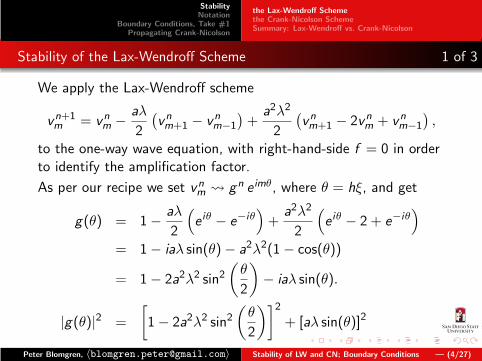
Stability of the Lax-Wendroff Scheme 1 of 3
We apply the Lax-Wendroff scheme
vn+1m = vnm −
aλ
2
(vnm+1 − vnm−1
)+
a2λ2
2
(vnm+1 − 2vnm + vnm−1
),
to the one-way wave equation, with right-hand-side f = 0 in orderto identify the amplification factor.
Peter Blomgren, 〈[email protected]〉 Stability of LW and CN; Boundary Conditions — (4/27)
StabilityNotation
Boundary Conditions, Take #1Propagating Crank-Nicolson
the Lax-Wendroff Schemethe Crank-Nicolson SchemeSummary: Lax-Wendroff vs. Crank-Nicolson
Stability of the Lax-Wendroff Scheme 1 of 3
We apply the Lax-Wendroff scheme
vn+1m = vnm −
aλ
2
(vnm+1 − vnm−1
)+
a2λ2
2
(vnm+1 − 2vnm + vnm−1
),
to the one-way wave equation, with right-hand-side f = 0 in orderto identify the amplification factor.
As per our recipe we set vnm gn e imθ, where θ = hξ, and get
g(θ) = 1−aλ
2
(
e iθ − e−iθ)
+a2λ2
2
(
e iθ − 2 + e−iθ)
= 1− iaλ sin(θ)− a2λ2(1− cos(θ))
= 1− 2a2λ2 sin2(θ
2
)
− iaλ sin(θ).
|g(θ)|2 =
[
1− 2a2λ2 sin2(θ
2
)]2
+ [aλ sin(θ)]2
Peter Blomgren, 〈[email protected]〉 Stability of LW and CN; Boundary Conditions — (4/27)
StabilityNotation
Boundary Conditions, Take #1Propagating Crank-Nicolson
the Lax-Wendroff Schemethe Crank-Nicolson SchemeSummary: Lax-Wendroff vs. Crank-Nicolson
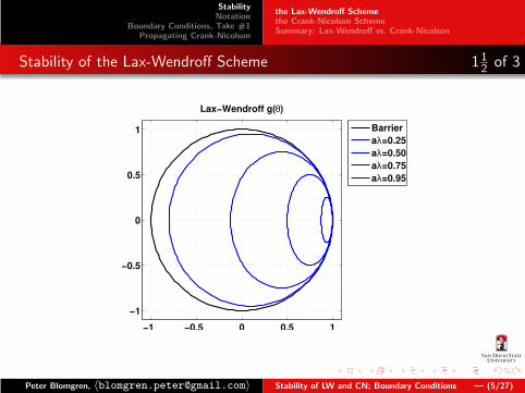
Stability of the Lax-Wendroff Scheme 112 of 3
−1 −0.5 0 0.5 1
−1
−0.5
0
0.5
1
Lax−Wendroff g(θ)
Barrier
aλ=0.25
aλ=0.50
aλ=0.75
aλ=0.95
Peter Blomgren, 〈[email protected]〉 Stability of LW and CN; Boundary Conditions — (5/27)
StabilityNotation
Boundary Conditions, Take #1Propagating Crank-Nicolson
the Lax-Wendroff Schemethe Crank-Nicolson SchemeSummary: Lax-Wendroff vs. Crank-Nicolson
Stability of the Lax-Wendroff Scheme 2 of 3
|g(θ)|2 =
[
1− 2a2λ2 sin2(θ
2
)]2
+ [aλ sin(θ)]2
=
[
1− 2a2λ2 sin2(θ
2
)]2
+
[
2aλ sin
(θ
2
)
cos
(θ
2
)]2
= 1− 4a2λ2 sin2(θ
2
)
+ 4a4λ4 sin4(θ
2
)
+4a2λ2 sin2(θ
2
)
cos2(θ
2
)
= 1− 4a2λ2 sin2(θ
2
)[
1− cos2(θ
2
)]
+ 4a4λ4 sin4(θ
2
)
= 1− 4a2λ2 sin4(θ
2
)
+ 4a4λ4 sin4(θ
2
)
= 1− 4a2λ2[1− a2λ2
]sin4
(θ
2
)
Peter Blomgren, 〈[email protected]〉 Stability of LW and CN; Boundary Conditions — (6/27)
StabilityNotation
Boundary Conditions, Take #1Propagating Crank-Nicolson
the Lax-Wendroff Schemethe Crank-Nicolson SchemeSummary: Lax-Wendroff vs. Crank-Nicolson
Stability of the Lax-Wendroff Scheme 3 of 3
|g(θ)|2 = 1− 4a2λ2[1− a2λ2
]sin4
(θ
2
)
︸ ︷︷ ︸
γ(θ)
In order for |g(θ)| ≤ 1, we must have that 0 ≤ γ(θ) ≤ 2. Thisgives us the condition |aλ| ≤ 1. �
At this point we know
Lax-Wendroff
Mode ExplicitOrder of Accuracy (2,2)Stability Criterion |aλ| ≤ 1 (CFL)
Peter Blomgren, 〈[email protected]〉 Stability of LW and CN; Boundary Conditions — (7/27)
StabilityNotation
Boundary Conditions, Take #1Propagating Crank-Nicolson
the Lax-Wendroff Schemethe Crank-Nicolson SchemeSummary: Lax-Wendroff vs. Crank-Nicolson
Stability of the Crank-Nicolson Scheme 1 of 2
After the excitement of verifying the stability for the Lax-Wendroffscheme, we now attack the Crank-Nicolson scheme
vn+1m − vnm
k+ a
vn+1m+1 − vn+1
m−1 + vnm+1 − vnm−1
4h= 0,
with the same toolbox.
The usual vnm gn e imθ, gives us
g − 1
k+ a
g(e iθ − e−iθ) + (e iθ − e−iθ)
4h= 0,
so that
g − 1 + iaλ(g + 1) sin(θ)
2= 0.
Peter Blomgren, 〈[email protected]〉 Stability of LW and CN; Boundary Conditions — (8/27)
StabilityNotation
Boundary Conditions, Take #1Propagating Crank-Nicolson
the Lax-Wendroff Schemethe Crank-Nicolson SchemeSummary: Lax-Wendroff vs. Crank-Nicolson
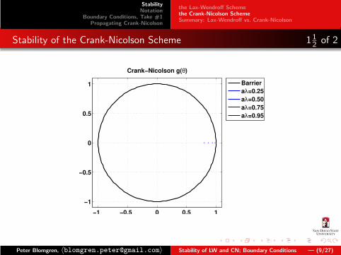
Stability of the Crank-Nicolson Scheme 112 of 2
−1 −0.5 0 0.5 1
−1
−0.5
0
0.5
1
Crank−Nicolson g(θ)
Barrier
aλ=0.25
aλ=0.50
aλ=0.75
aλ=0.95
Peter Blomgren, 〈[email protected]〉 Stability of LW and CN; Boundary Conditions — (9/27)
StabilityNotation
Boundary Conditions, Take #1Propagating Crank-Nicolson
the Lax-Wendroff Schemethe Crank-Nicolson SchemeSummary: Lax-Wendroff vs. Crank-Nicolson
Stability of the Crank-Nicolson Scheme 2 of 2
We write
g − 1 + iaλ(g + 1) sin(θ)
2= 0,
as
g
[
1 +iaλ
2sin(θ)
]
−
[
1−iaλ
2sin(θ)
]
= 0.
Finally,
g(θ) =1− iaλ
2 sin(θ)
1 + iaλ2 sin(θ)
, |g(θ)|2 =1+ a2λ2
4 sin2(θ)
1+ a2λ2
4 sin2(θ)= 1.
Peter Blomgren, 〈[email protected]〉 Stability of LW and CN; Boundary Conditions — (10/27)
StabilityNotation
Boundary Conditions, Take #1Propagating Crank-Nicolson
the Lax-Wendroff Schemethe Crank-Nicolson SchemeSummary: Lax-Wendroff vs. Crank-Nicolson
Stability of the Crank-Nicolson Scheme 2 of 2
We write
g − 1 + iaλ(g + 1) sin(θ)
2= 0,
as
g
[
1 +iaλ
2sin(θ)
]
−
[
1−iaλ
2sin(θ)
]
= 0.
Finally,
g(θ) =1− iaλ
2 sin(θ)
1 + iaλ2 sin(θ)
, |g(θ)|2 =1+ a2λ2
4 sin2(θ)
1+ a2λ2
4 sin2(θ)= 1.
Hence,
Property: Unconditional Stability of Crank-Nicolson
The Crank-Nicolson scheme is stable for any value of aλ, we saythat it is unconditionally stable.
Peter Blomgren, 〈[email protected]〉 Stability of LW and CN; Boundary Conditions — (10/27)
StabilityNotation
Boundary Conditions, Take #1Propagating Crank-Nicolson
the Lax-Wendroff Schemethe Crank-Nicolson SchemeSummary: Lax-Wendroff vs. Crank-Nicolson
The Lax-Wendroff scheme is easier to propagate (since it isexplicit), but if the speed a is large, the stability criterion mayimpose a severe time-step restriction, recall k = h/|a|.
The fact that the Crank-Nicolson scheme is unconditionally stablemakes it (and variants) extremely useful; the only down-side is thatfor each time-step we must solve a linear system Av̄n+1 = b̄n(v̄
n).
Peter Blomgren, 〈[email protected]〉 Stability of LW and CN; Boundary Conditions — (11/27)
StabilityNotation
Boundary Conditions, Take #1Propagating Crank-Nicolson
Difference Notation and the Difference Calculus
Difference Notation and the Difference Calculus
We introduce the following notation
δ+vm =vm+1 − vm
h︸ ︷︷ ︸
Forward Difference
, δ−vm =vm − vm−1
h︸ ︷︷ ︸
Backward Difference
δ0vm =1
2(δ+ + δ−)vm =
vm+1 − vm−1
2h︸ ︷︷ ︸
Central Difference
.
Further, we can define the second difference operatorδ2 = δ+δ− ≡ δ+−δ−
h:
δ2vm =vm+1 − 2vm + vm−1
h2.
We can define the corresponding time-differences δt+, δt−, δt0,and δ2t ...
Peter Blomgren, 〈[email protected]〉 Stability of LW and CN; Boundary Conditions — (12/27)
StabilityNotation
Boundary Conditions, Take #1Propagating Crank-Nicolson
Difference Notation and the Difference Calculus
What’s The Use??? — Deriving Higher-Order Approximations
Consider the Taylor expansion of the central difference operator
δ0u =du
dx+
h2
6
d3u
dx3+O
(h4)=
[
1 +h2
6δ2]du
dx+O
(h4)
where, in the second equality we have used
δ2u =d2u
dx2+O
(h2).
Now, formally (symbolically)
du
dx=
[
1 +h2
6δ2]−1
δ0u +O(h4).
The inverse operator [◦]−1 is (almost) always eliminated byoperating on both sides with the operator [◦] itself...
Peter Blomgren, 〈[email protected]〉 Stability of LW and CN; Boundary Conditions — (13/27)
StabilityNotation
Boundary Conditions, Take #1Propagating Crank-Nicolson
Difference Notation and the Difference Calculus
Example: A Fourth Order Approximation to ux = f
Applying what we have developed to the equation
du
dx= f ,
we get
[
1 +h2
6δ2]−1
δ0vm = fm (1)
δ0vm =
[
1 +h2
6δ2]
fm (2)
vm+1 − vm−1
2h= fm +
1
6[fm+1 − 2fm + fm−1] (3)
=1
6[fm+1 + 4fm + fm−1] .
If/When the right-hand-side is simply fm, we only have a second orderapproximation...
Peter Blomgren, 〈[email protected]〉 Stability of LW and CN; Boundary Conditions — (14/27)
StabilityNotation
Boundary Conditions, Take #1Propagating Crank-Nicolson
Difference Notation and the Difference Calculus
Example: Another Possibility — 4th Order Scheme
We can go a slightly different route:
δ0u =du
dx+
h2
6
d3u
dx3+O
(h4)=
du
dx+
h2
6δ2δ0u +O
(h4),
so that
[
1−h2
6δ2]
δ0u =du
dx+O
(h4).
From which we get the fourth order scheme
−vm+2 + 8vm+1 − 8vm−1 + vm−2
12h= fm.
Clearly, this notation may come in handy...
Peter Blomgren, 〈[email protected]〉 Stability of LW and CN; Boundary Conditions — (15/27)
StabilityNotation
Boundary Conditions, Take #1Propagating Crank-Nicolson
Examples of Numerical Boundary Conditions
Boundary Conditions — Physical
We have seen that when we solve IVPsin finite physical domains, we need physi-cal boundary conditions at the boundarieswhere characteristics enter the domain.— This corresponds to a physical process,such as keeping a temperature constant (orvarying in time), regulating the flow of waterthrough the turbines in a dam, the absorp-tion of sound in the ceiling and walls of yoursubterranean media room...
Clearly, a numerical scheme must accurately capture these physicalboundary conditions.
Peter Blomgren, 〈[email protected]〉 Stability of LW and CN; Boundary Conditions — (16/27)
StabilityNotation
Boundary Conditions, Take #1Propagating Crank-Nicolson
Examples of Numerical Boundary Conditions
Boundary Conditions — (Additional) Numerical
Further, many numerical schemes also require additional boundaryconditions, called numerical boundary conditions in order for thesolution to be well defined (unique).
Numerical boundary conditions often arise for reasons similar tothe ones that impose the need for additional numerical initialconditions (for multi-step schemes) and/or to make a finitecomputational domain “act” infinite.
Dealing with boundary conditions, physical and/or numerical ismany times the most difficult part of simulating a PDE.
Peter Blomgren, 〈[email protected]〉 Stability of LW and CN; Boundary Conditions — (17/27)
StabilityNotation
Boundary Conditions, Take #1Propagating Crank-Nicolson
Examples of Numerical Boundary Conditions
Boundary Conditions
For our discussion we use the Lax-Wendroff scheme
vn+1m = vnm −
aλ
2
(vnm+1 − vnm−1
)+
a2λ2
2
(vnm+1 − 2vnm + vnm−1
),
applied to the equation
ut + aux = 0, 0 ≤ x ≤ 1, t ≥ 0.
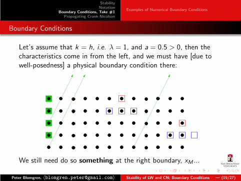
But, we run into problems at the boundaries, some points are“missing:”
Peter Blomgren, 〈[email protected]〉 Stability of LW and CN; Boundary Conditions — (18/27)
StabilityNotation
Boundary Conditions, Take #1Propagating Crank-Nicolson
Examples of Numerical Boundary Conditions
Boundary Conditions
Let’s assume that k = h, i.e. λ = 1, and a = 0.5 > 0, then thecharacteristics come in from the left, and we must have [due towell-posedness] a physical boundary condition there:
We still need do so something at the right boundary, xM ...
Peter Blomgren, 〈[email protected]〉 Stability of LW and CN; Boundary Conditions — (19/27)
StabilityNotation
Boundary Conditions, Take #1Propagating Crank-Nicolson
Examples of Numerical Boundary Conditions
Examples of Numerical Boundary Conditions
Here are some possibilities:
vn+1M = vn+1
M−1 (1)
vn+1M = 2vn+1
M−1 − vn+1M−2 (2)
vn+1M = vn
M−1 (3)
vn+1M = 2vn
M−1 − vn−1M−2 (4)
Formulas (1) and (2) are simple extrapolations of interior grid points tothe boundary. Formulas (3) and (4) are referred to asquasi-characteristic extrapolation, since the extrapolation uses points“near” the characteristics. Usually, but not always, it is better to useone-sided difference formulas at the boundaries, i.e.
vn+1M = vn
M − aλ(vnM − vn
M−1). (5)
Peter Blomgren, 〈[email protected]〉 Stability of LW and CN; Boundary Conditions — (20/27)
StabilityNotation
Boundary Conditions, Take #1Propagating Crank-Nicolson
Examples of Numerical Boundary Conditions
Problems that Can Occur Accuracy & Stability
The decision on what to do at the boundary may seem like a smallone... We’re only talking about what to do at one point, and quitepossibly we may have thousands or billions of interior points...
However, any error we introduce at the boundary willeventually affect the entire solution:
If we have a 4th order scheme (in the interior), but use a sloppy1st order one-sided difference at the boundary, then the overallscheme is only 1st order.
In addition, the boundary condition will affect the stability ofthe scheme!
We will re-visit these issues again (and again), in more detail; fornow, we ponder the table on the next slide.
Peter Blomgren, 〈[email protected]〉 Stability of LW and CN; Boundary Conditions — (21/27)
StabilityNotation
Boundary Conditions, Take #1Propagating Crank-Nicolson
The effect of incorrect boundary conditions are usually oscillations in thesolution. These oscillations may be observed away from the boundary,which makes it hard to correctly diagnose the cause of the problem.
Usually, if you suspect that an unstable numerical boundary condition iscausing instability, the easiest way to pinpoint the problem is to changethe boundary condition and observe the solution.
We will return to the analysis of boundary conditions, but we need more(mathematical) tools before we do so.
Peter Blomgren, 〈[email protected]〉 Stability of LW and CN; Boundary Conditions — (22/27)
StabilityNotation
Boundary Conditions, Take #1Propagating Crank-Nicolson
Solving Tridiagonal SystemsThe Thomas Algorithm Math 541
Propagating Crank-Nicolson: Solving Tridiagonal Systems 1 of 3
We now return to the issue of propagating the Crank-Nicolsonscheme
vn+1m − vnm
k+ a
vn+1m+1 − vn+1
m−1 + vnm+1 − vnm−1
4h= 0.
We rewrite this so we have all the unknown terms to the left, andthe known terms to the right
−[ a
4h
]
vn+1m−1+
[1
k
]
vn+1m +
[ a
4h
]
vn+1m+1 =
a
4hvnm−1 +
1
kvnm −
a
4hvnm+1
︸ ︷︷ ︸
bnm
,
where if the x-grid is given by x0, x1, . . . , xM , the index m runsfrom 1 to (M − 1), and we apply appropriate boundary conditionsat x0 and xM .
Peter Blomgren, 〈[email protected]〉 Stability of LW and CN; Boundary Conditions — (23/27)
StabilityNotation
Boundary Conditions, Take #1Propagating Crank-Nicolson
Solving Tridiagonal SystemsThe Thomas Algorithm Math 541
Propagating Crank-Nicolson: Solving Tridiagonal Systems 2 of 3
This gives rise to a tri-diagonal system
1 0−α β α
. . .. . .
. . .
−α β α0 −1 1
v0v1...
vM−1
vM
n+1
=
b0b1...
bM−1
0
n
where α = a/4h, β = 1/k ; bn0 = ϕ(tn+1) is the specification of thephysical boundary condition at (tn+1, x0); the last row−vM−1 + vM = 0 corresponds to (BC-1 on slide 20); and bn1through bnM−1 are computed according to the previous slide.
Peter Blomgren, 〈[email protected]〉 Stability of LW and CN; Boundary Conditions — (24/27)
StabilityNotation
Boundary Conditions, Take #1Propagating Crank-Nicolson
Solving Tridiagonal SystemsThe Thomas Algorithm Math 541
Propagating Crank-Nicolson: Solving Tridiagonal Systems 3 of 3
A tri-diagonal system like this can be solved on O (M) operations,which should be compared with the more general requirementO(M3
)for a full matrix. The Thomas Algorithm is discussed in
Math 541, and is also presented in Strikwerda.
A matlab implementation (without error checking, for brevity) ispresented on the next slide.
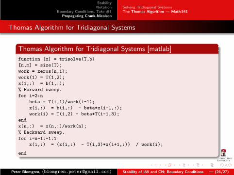
In order for the algorithm to work, the tridiagonal matrix T “mustbe in compact form: the sub-diagonal elements in the firstcolumn, the diagonal in the second column, and thesuper-diagonal in the third column. [...] Note that T(1,1)and T(n,3) are never accessed, i.e. the sub-diagonal entriesstart on the second row, and the super-diagonal elementsend on the (n-1)st row.”
Peter Blomgren, 〈[email protected]〉 Stability of LW and CN; Boundary Conditions — (25/27)
StabilityNotation
Boundary Conditions, Take #1Propagating Crank-Nicolson
Solving Tridiagonal SystemsThe Thomas Algorithm Math 541
Thomas Algorithm for Tridiagonal Systems
Thomas Algorithm for Tridiagonal Systems [matlab]
function [x] = trisolve(T,b)
[n,m] = size(T);
work = zeros(n,1);
work(1) = T(1,2);
x(1,:) = b(1,:);
% Forward sweep.
for i=2:n
beta = T(i,1)/work(i-1);
x(i,:) = b(i,:) - beta*x(i-1,:);
work(i) = T(i,2) - beta*T(i-1,3);
end
x(n,:) = x(n,:)/work(n);
% Backward sweep.
for i=n-1:-1:1
x(i,:) = (x(i,:) - T(i,3)*x(i+1,:)) / work(i);
end
Peter Blomgren, 〈[email protected]〉 Stability of LW and CN; Boundary Conditions — (26/27)
StabilityNotation
Boundary Conditions, Take #1Propagating Crank-Nicolson
Solving Tridiagonal SystemsThe Thomas Algorithm Math 541
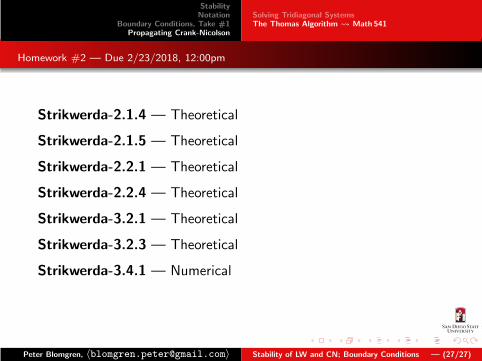
Homework #2 — Due 2/23/2018, 12:00pm
Strikwerda-2.1.4 — Theoretical
Strikwerda-2.1.5 — Theoretical
Strikwerda-2.2.1 — Theoretical
Strikwerda-2.2.4 — Theoretical
Strikwerda-3.2.1 — Theoretical
Strikwerda-3.2.3 — Theoretical
Strikwerda-3.4.1 — Numerical
Peter Blomgren, 〈[email protected]〉 Stability of LW and CN; Boundary Conditions — (27/27)