Numerical study of bubble break-up in bubbly flows using a deterministic Euler–Lagrange framework Y.M. Lau, W. Bai, N.G. Deen n , J.A.M. Kuipers Multiphase Reactors Group, Department of Chemical Engineering and Chemistry, Eindhoven University of Technology, P.O. Box 513, 5600 MB, Eindhoven, The Netherlands HIGHLIGHTS A simulation framework for hetero- geneous bubbly flow is presented. A Lagrangian breakup model is pro- posed. The daughter size distribution does not influence the bubble size distribution (BSD). The critical Weber number and superficial gas velocity significantly affect the BSD. GRAPHICAL ABSTRACT article info Article history: Received 26 July 2013 Received in revised form 26 November 2013 Accepted 23 December 2013 Available online 2 January 2014 Keywords: Euler–Lagrange model Bubble columns Coalescence Break-up Daughter size distribution abstract In this work we present a numerical model to predict the bubble size distribution in turbulent bubbly flows. The continuous phase is described by the volume-averaged Navier–Stokes equations, which are solved on an Eulerian grid, whereas the dispersed or bubble phase is treated in a Lagrangian manner, where each individual bubble is tracked throughout the computational domain. Collisions between bubbles are described by means of a hard-sphere model. Coalescence of bubbles is modeled via a stochastic inter-particle encounter model. A break-up model is implemented with a break-up constraint on the basis of a critical Weber value augmented with a model for the daughter size distribution. A numerical parameter study is performed of the bubble break-up model implemented in the deterministic Euler–Lagrange framework and its effect on the bubble size distribution (BSD) is reported. A square bubble column operated at a superficial gas velocity of 2 cm/s is chosen as a simulation base case to evaluate the parameters. The parameters that are varied are the values of the critical Weber number (We crit ), the daughter size distribution (β) and the superficial gas velocity (v sup ). Changes in the values of We crit and v sup have a significant impact on the overall BSD, while a different shaped β did not show a significant difference. & 2014 Elsevier Ltd. All rights reserved. 1. Introduction In turbulent bubbly flows, coalescence and break-up of bubbles determine the bubble size distribution and the corresponding interfacial area. Hence, these phenomena play a crucial role in mass and heat transfer operations in bubbly flows. To predict the bubble size distribution in industrial bubbly flows, the population balance equation (PBE) embedded in the Euler–Euler model is often used. Traditionally the Euler–Euler model treats the dis- persed gas phase as a separate continuum with averaged proper- ties, i.e. mean bubble diameter. The disadvantage is that the information regarding individual bubbles is not available. To retain the bubble size distribution a PBE is employed. The PBE handles the evolution of the size distribution of the dispersed phase Contents lists available at ScienceDirect journal homepage: www.elsevier.com/locate/ces Chemical Engineering Science 0009-2509/$ - see front matter & 2014 Elsevier Ltd. All rights reserved. http://dx.doi.org/10.1016/j.ces.2013.12.034 n Corresponding author. E-mail address: [email protected](N.G. Deen). Chemical Engineering Science 108 (2014) 9–22
Transcript
Numerical study of bubble break-up in bubbly flows usinga deterministic Euler–Lagrange framework
Y.M. Lau, W. Bai, N.G. Deen n, J.A.M. KuipersMultiphase Reactors Group, Department of Chemical Engineering and Chemistry, Eindhoven University of Technology, P.O. Box 513, 5600 MB, Eindhoven,The Netherlands
H I G H L I G H T S
� A simulation framework for hetero-geneous bubbly flow is presented.
� A Lagrangian breakup model is pro-posed.
� The daughter size distribution doesnot influence the bubble sizedistribution (BSD).
� The critical Weber number andsuperficial gas velocity significantlyaffect the BSD.
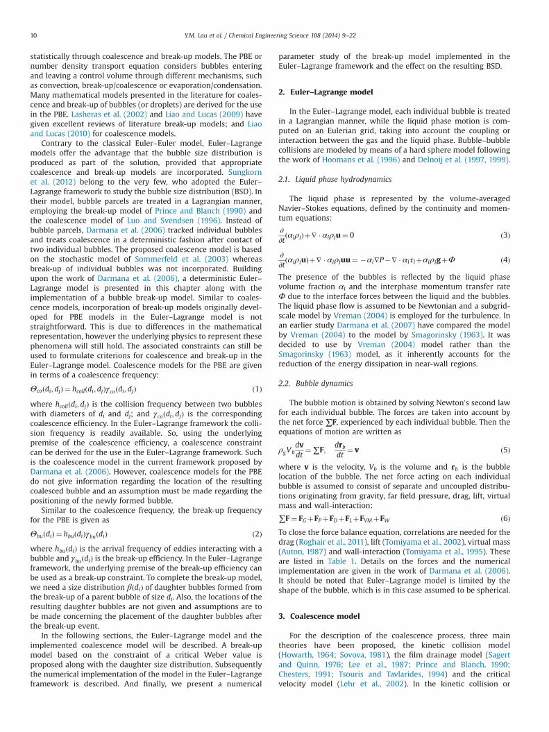
G R A P H I C A L A B S T R A C T
a r t i c l e i n f o
Article history:Received 26 July 2013Received in revised form26 November 2013Accepted 23 December 2013Available online 2 January 2014
Keywords:Euler–Lagrange modelBubble columnsCoalescenceBreak-upDaughter size distribution
a b s t r a c t
In this work we present a numerical model to predict the bubble size distribution in turbulent bubblyflows. The continuous phase is described by the volume-averaged Navier–Stokes equations, which aresolved on an Eulerian grid, whereas the dispersed or bubble phase is treated in a Lagrangian manner,where each individual bubble is tracked throughout the computational domain. Collisions betweenbubbles are described by means of a hard-sphere model. Coalescence of bubbles is modeled via astochastic inter-particle encounter model. A break-up model is implemented with a break-up constrainton the basis of a critical Weber value augmented with a model for the daughter size distribution.A numerical parameter study is performed of the bubble break-up model implemented in thedeterministic Euler–Lagrange framework and its effect on the bubble size distribution (BSD) is reported.A square bubble column operated at a superficial gas velocity of 2 cm/s is chosen as a simulation basecase to evaluate the parameters. The parameters that are varied are the values of the critical Webernumber (Wecrit), the daughter size distribution (β) and the superficial gas velocity (vsup). Changes in thevalues of Wecrit and vsup have a significant impact on the overall BSD, while a different shaped β did notshow a significant difference.
& 2014 Elsevier Ltd. All rights reserved.
1. Introduction
In turbulent bubbly flows, coalescence and break-up of bubblesdetermine the bubble size distribution and the correspondinginterfacial area. Hence, these phenomena play a crucial role in
mass and heat transfer operations in bubbly flows. To predict thebubble size distribution in industrial bubbly flows, the populationbalance equation (PBE) embedded in the Euler–Euler model isoften used. Traditionally the Euler–Euler model treats the dis-persed gas phase as a separate continuum with averaged proper-ties, i.e. mean bubble diameter. The disadvantage is that theinformation regarding individual bubbles is not available. To retainthe bubble size distribution a PBE is employed. The PBE handlesthe evolution of the size distribution of the dispersed phase
Contents lists available at ScienceDirect
journal homepage: www.elsevier.com/locate/ces
Chemical Engineering Science
0009-2509/$ - see front matter & 2014 Elsevier Ltd. All rights reserved.http://dx.doi.org/10.1016/j.ces.2013.12.034
n Corresponding author.E-mail address: [email protected] (N.G. Deen).
statistically through coalescence and break-up models. The PBE ornumber density transport equation considers bubbles enteringand leaving a control volume through different mechanisms, suchas convection, break-up/coalescence or evaporation/condensation.Many mathematical models presented in the literature for coales-cence and break-up of bubbles (or droplets) are derived for the usein the PBE. Lasheras et al. (2002) and Liao and Lucas (2009) havegiven excellent reviews of literature break-up models; and Liaoand Lucas (2010) for coalescence models.
Contrary to the classical Euler–Euler model, Euler–Lagrangemodels offer the advantage that the bubble size distribution isproduced as part of the solution, provided that appropriatecoalescence and break-up models are incorporated. Sungkornet al. (2012) belong to the very few, who adopted the Euler–Lagrange framework to study the bubble size distribution (BSD). Intheir model, bubble parcels are treated in a Lagrangian manner,employing the break-up model of Prince and Blanch (1990) andthe coalescence model of Luo and Svendsen (1996). Instead ofbubble parcels, Darmana et al. (2006) tracked individual bubblesand treats coalescence in a deterministic fashion after contact oftwo individual bubbles. The proposed coalescence model is basedon the stochastic model of Sommerfeld et al. (2003) whereasbreak-up of individual bubbles was not incorporated. Buildingupon the work of Darmana et al. (2006), a deterministic Euler–Lagrange model is presented in this chapter along with theimplementation of a bubble break-up model. Similar to coales-cence models, incorporation of break-up models originally devel-oped for PBE models in the Euler–Lagrange model is notstraightforward. This is due to differences in the mathematicalrepresentation, however the underlying physics to represent thesephenomena will still hold. The associated constraints can still beused to formulate criterions for coalescence and break-up in theEuler–Lagrange model. Coalescence models for the PBE are givenin terms of a coalescence frequency:
Θcoðdi; djÞ ¼ hcollðdi; djÞγcoðdi; djÞ ð1Þ
where hcollðdi; djÞ is the collision frequency between two bubbleswith diameters of di and dj; and γcoðdi; djÞ is the correspondingcoalescence efficiency. In the Euler–Lagrange framework the colli-sion frequency is readily available. So, using the underlyingpremise of the coalescence efficiency, a coalescence constraintcan be derived for the use in the Euler–Lagrange framework. Suchis the coalescence model in the current framework proposed byDarmana et al. (2006). However, coalescence models for the PBEdo not give information regarding the location of the resultingcoalesced bubble and an assumption must be made regarding thepositioning of the newly formed bubble.
Similar to the coalescence frequency, the break-up frequencyfor the PBE is given as
ΘbuðdiÞ ¼ hbuðdiÞγbuðdiÞ ð2Þwhere hbuðdiÞ is the arrival frequency of eddies interacting with abubble and γbuðdiÞ is the break-up efficiency. In the Euler–Lagrangeframework, the underlying premise of the break-up efficiency canbe used as a break-up constraint. To complete the break-up model,we need a size distribution βðdiÞ of daughter bubbles formed fromthe break-up of a parent bubble of size di. Also, the locations of theresulting daughter bubbles are not given and assumptions are tobe made concerning the placement of the daughter bubbles afterthe break-up event.
In the following sections, the Euler–Lagrange model and theimplemented coalescence model will be described. A break-upmodel based on the constraint of a critical Weber value isproposed along with the daughter size distribution. Subsequentlythe numerical implementation of the model in the Euler–Lagrangeframework is described. And finally, we present a numerical
parameter study of the break-up model implemented in theEuler–Lagrange framework and the effect on the resulting BSD.
2. Euler–Lagrange model
In the Euler–Lagrange model, each individual bubble is treatedin a Lagrangian manner, while the liquid phase motion is com-puted on an Eulerian grid, taking into account the coupling orinteraction between the gas and the liquid phase. Bubble–bubblecollisions are modeled by means of a hard sphere model followingthe work of Hoomans et al. (1996) and Delnoij et al. (1997, 1999).
2.1. Liquid phase hydrodynamics
The liquid phase is represented by the volume-averagedNavier–Stokes equations, defined by the continuity and momen-tum equations:
∂∂tðαlρlÞþ∇ � αlρlu¼ 0 ð3Þ
∂∂tðαlρluÞþ∇ � αlρluu¼ �αl∇P�∇ � αlτlþαlρlgþΦ ð4Þ
The presence of the bubbles is reflected by the liquid phasevolume fraction αl and the interphase momentum transfer rateΦ due to the interface forces between the liquid and the bubbles.The liquid phase flow is assumed to be Newtonian and a subgrid-scale model by Vreman (2004) is employed for the turbulence. Inan earlier study Darmana et al. (2007) have compared the modelby Vreman (2004) to the model by Smagorinsky (1963). It wasdecided to use by Vreman (2004) model rather than theSmagorinsky (1963) model, as it inherently accounts for thereduction of the energy dissipation in near-wall regions.
2.2. Bubble dynamics
The bubble motion is obtained by solving Newton0s second lawfor each individual bubble. The forces are taken into account bythe net force ∑F, experienced by each individual bubble. Then theequations of motion are written as
ρgVbdvdt
¼∑F;drbdt
¼ v ð5Þ
where v is the velocity, Vb is the volume and rb is the bubblelocation of the bubble. The net force acting on each individualbubble is assumed to consist of separate and uncoupled distribu-tions originating from gravity, far field pressure, drag, lift, virtualmass and wall-interaction:
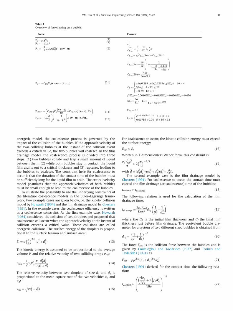
∑F¼ FGþFPþFDþFLþFVMþFW ð6ÞTo close the force balance equation, correlations are needed for thedrag (Roghair et al., 2011), lift (Tomiyama et al., 2002), virtual mass(Auton, 1987) and wall-interaction (Tomiyama et al., 1995). Theseare listed in Table 1. Details on the forces and the numericalimplementation are given in the work of Darmana et al. (2006).It should be noted that Euler–Lagrange model is limited by theshape of the bubble, which is in this case assumed to be spherical.
3. Coalescence model
For the description of the coalescence process, three maintheories have been proposed, the kinetic collision model(Howarth, 1964; Sovova, 1981), the film drainage model (Sagertand Quinn, 1976; Lee et al., 1987; Prince and Blanch, 1990;Chesters, 1991; Tsouris and Tavlarides, 1994) and the criticalvelocity model (Lehr et al., 2002). In the kinetic collision or
Y.M. Lau et al. / Chemical Engineering Science 108 (2014) 9–2210
energetic model, the coalescence process is governed by theimpact of the collision of the bubbles. If the approach velocity ofthe two colliding bubbles at the instant of the collision eventexceeds a critical value, the two bubbles will coalesce. In the filmdrainage model, the coalescence process is divided into threesteps: (1) two bubbles collide and trap a small amount of liquidbetween them; (2) while both bubbles stay in contact, the liquidfilm drains out to a critical thickness and (3) ruptures, leading tothe bubbles to coalesce. The constraint here for coalescence tooccur is that the duration of the contact time of the bubbles mustbe sufficiently long for the liquid film to drain. The critical velocitymodel postulates that the approach velocities of both bubblesmust be small enough to lead to the coalescence of the bubbles.
To illustrate the possibility to use the underlying constraints ofthe literature coalescence models in the Euler–Lagrange frame-work, two example cases are given below, i.e. the kinetic collisionmodel by Howarth (1964) and the film drainage model by Chesters(1991). In the example cases the coalescence efficiency is writtenas a coalescence constraint. As the first example case, Howarth(1964) considered the collision of two droplets and proposed thatcoalescence will occur when the approach velocity at the instant ofcollision exceeds a critical value. These collisions are calledenergetic collisions. The surface energy of the droplets is propor-tional to the surface tension and surface area:
Es ¼ s π6
� �2=3ðd21þd22Þ ð13Þ
The kinetic energy is assumed to be proportional to the averagevolume V and the relative velocity of two colliding drops vrel:
Ekin ¼12ρgv
2relπ6
d31d32
d31þd32ð14Þ
The relative velocity between two droplets of size d1 and d2 isproportional to the mean-square root of the two velocities v1 andv2:
For coalescence to occur, the kinetic collision energy must exceedthe surface energy:
Ekin4Es ð16ÞWritten in a dimensionless Weber form, this constraint is
ρgv2relds 42
π6
� ��1=3ð17Þ
with d ¼ ðd31d32Þ=ððd21þd22Þðd31þd32ÞÞ.The second example case is the film drainage model by
Chesters (1991). For coalescence to occur, the contact time mustexceed the film drainage (or coalescence) time of the bubbles:
tcontactZtdrainage ð18Þ
The following relation is used for the calculation of the filmdrainage time:
tdrainage ¼3μcFcoll8πs2 deq
1
θ2f
� 1
θ20
!ð19Þ
where the θ0 is the initial film thickness and θf the final filmthickness just before film drainage. The equivalent bubble dia-meter for a system of two different sized bubbles is obtained from
deq ¼ 1d1
þ 1d2
� ��1
ð20Þ
The force Fcoll is the collision force between the bubbles and isgiven by Coulaloglou and Tavlarides (1977) and Tsouris andTavlarides (1994) as
Fcoll � ρlɛ2=3ðd1þd2Þ2=3d2eq ð21Þ
Chesters (1991) derived for the contact time the following rela-tion:
Y.M. Lau et al. / Chemical Engineering Science 108 (2014) 9–22 11
Since the collision frequency is readily available in the Euler–Lagrange model, the coalescence constraints of the example cases,Eqs. (16) and (18) can be evaluated for each bubble–bubbleencounter. In this work we use the film drainage model asimplemented by Darmana et al. (2006). For the drainage timethe relation of Prince and Blanch (1990) is used:
tdrainage ¼
ffiffiffiffiffiffiffiffiffiffiffiffid3eqρl
128s
sln
θ0
θf
!ð23Þ
According to Sommerfeld et al. (2003), the contact time betweentwo bubbles is calculated by assuming that it is proportional to adeformation distance divided by the normal component of thecollision velocity:
tcontact ¼Ccodeq
2jvN1 �vN2 j
ð24Þ
where the coalescence constant (Cco) represents the deformationdistance normalized by the effective bubble diameter. The criteriafor the occurrence of coalescence or collision (and bounce off) aredetermined by the ratio of the contact time and the film drainagetime tcontact=tdrainage. Written in a dimensionless Weber form, thisconstraint is
We¼ ρlðvN1 �vN2 Þ2deq
s r2 � 4Cco
lnθ0
θf
!0BBBB@
1CCCCA
2
ð25Þ
4. Break-up model
Break-up mechanisms can be classified into four main cate-gories regarding the governing physical process: turbulent fluc-tuation and collision; viscous shear stress; shearing off processand interfacial instability. From these mechanisms, bubble break-up due to turbulent pressure fluctuation along the surface or bycollision with eddies has been investigated most extensively. Thismechanism is assumed to be the dominant break-up mechanismin our case involving turbulent bubbly flows.
Concerning the break-up criteria itself, four different criteriahave been reported in the literature. The associated critical valuesinvolve the turbulent kinetic energy of the bubble (Coulaloglouand Tavlarides, 1977; Chatzi et al., 1989; Chatzi and Kiparissides,1992), the velocity fluctuation around the bubble surface(Narsimhan and Gupta, 1979; Alopaeus et al., 2002), the turbulentkinetic energy of the impacting eddy (Lee et al., 1987; Prince andBlanch, 1990; Tsouris and Tavlarides, 1994; Luo and Svendsen,1996; Martínez-Bazán et al., 1999) and the inertial force of theimpacting eddy (Lehr et al., 2002). According to these models, ifeach one of the mentioned energies or forces exceeds the criticalvalue, the bubble breaks up. In the following section, we will showthat the above-mentioned models can be written in terms of acritical Weber number. This critical Weber number can subse-quently be used as a break-up constraint for an individual bubble.
4.1. Break-up constraint
4.1.1. Literature models for break-up criteriaHinze (1955) is one of the first to establish a break-up theory by
introducing a dimensionless ratio between the inertial force(which causes deformation) and the surface tension (which tendsto restore the bubble sphericity). In turbulent flows the deforma-tion is induced by inertia and the dimensionless number is known
as the Weber number:
We¼ ρδu2ðdÞds ð26Þ
where ρl is the density of the continuous phase and δu2ðdÞ is themean square velocity difference over a distance equal to thebubble diameter. Assuming isotropic turbulence (Kolmogorov,1949; Batchelor, 1951), the Weber number can also be written as
We¼ c1ρɛ2=3d5=3
s ð27Þ
In this subsection, the break-up constraints of selected literaturemodels are described and it is shown that all constraints can bewritten in the form of a dimensionless Weber number.
Coulaloglou and Tavlarides (1977) derived their break-upmodel for droplets, but many researchers have applied it as wellfor the break-up of bubbles. In their model, the basic premise isthat an oscillating bubble will break-up if the turbulent kineticenergy transmitted to the bubble by the turbulent eddies exceedsthe bubble surface energy. The bubble surface energy is given as
Es ¼ c2sd2 ð28Þ
With the assumption that the kinetic energy distribution of thedroplet is the same as that of the eddies, the mean turbulentkinetic energy is given as
Et ¼ c3ρd3u2ðdÞ ¼ c4ρɛ2=3d
11=3 ð29Þ
Therefore, the break-up of a droplet occurs if its turbulent kineticenergy Et exceeds the droplet surface energy Es:
Wecrit ¼ρɛ2=3d5=3
s Zc2c4
ð30Þ
Originally the density chosen in the above formulation was thedispersed phase density (Coulaloglou and Tavlarides, 1977), whichin the case of bubbly flow corresponds to the gas density.However, Lasheras et al. (2002) pointed out that the density ofthe continuous phase should be used, which is the liquid phase forbubbly flow.
Narsimhan and Gupta (1979) derived a break-up model fordroplets in liquid–liquid dispersions. They postulated that for theoccurrence of break-up, the kinetic energy 1=2u2
λ of the eddy with
a length scale λ arriving at the droplet surface must exceed theminimum increase of the surface energy for binary break-up,1=2u2
λZ1=2u2min respectively. The arriving eddies cause the droplet
to oscillate and break-up. Hence, the minimum increase of thesurface energy for binary break-up is provided by the kineticenergy of the oscillation of the droplet:
12ρπ6d3
� �� �u2min ¼ ð21=3�1Þsπd2 ð31Þ
This leads to the following break-up constraint:
Wecrit ¼ρu2
λds Z12ð21=3�1Þ ¼ 3:12 ð32Þ
As the break-up constraint, most statistical models employ thecriterion of the turbulent kinetic energy of the impacting eddyexceeding a critical value. Prince and Blanch (1990) used a criticalWeber value of 2.3 for air bubbles in water for the formulation oftheir break-up model. Another popular model was proposedwithout any model parameters by Luo and Svendsen (1996). Theydefined the increase in surface energy during break-up as thecritical value using the daughter size distribution for the
Y.M. Lau et al. / Chemical Engineering Science 108 (2014) 9–2212
formulation of the break-up constraint:
Wecrit ¼ρlɛ
2=3d5=3
s Z12cf
c5λd
� �11=3 ð33Þ
with cf ¼ f 2=3bv þð1� f bvÞ2=3 and the volumetric break-up fractionf bv ¼ V1=V0.
Martínez-Bazán et al. (1999) developed a model for the break-up of an air bubble in a fully developed turbulent water flow. Theypostulated that when the turbulent stresses from the velocityfluctuations exceed the surface restoring pressure of the bubble,the bubble will deform and eventually break-up. The surfacerestoring pressure of a bubble with a size d is
τsðdÞ ¼ 6sd
ð34Þ
The average deformation force per unit surface produced by theturbulent stresses resulting from the velocity fluctuations existingin the liquid between two points separated by a distance d can beestimated as
τtðdÞ ¼12c6ρðɛdÞ2=3 ð35Þ
The equality of both stresses defines the critical bubble diameterdb;crit, such that bubbles with dbodb;crit are stable and will neverbreak. Thus for break-up to occur, the following must be valid:
Wecrit ¼ρɛ2=3d5=3
s Z12c6
ð36Þ
Lehr et al. (2002) proposed to use the interfacial force of thesmallest daughter bubble as the critical value for inertial force ofthe impacting turbulent eddy:
Wecrit ¼ρluλdsmallest daughter
s Z4 ð37Þ
Using the assumption that only eddies with length scales smallerthan the bubble diameter can induce break-up, the followingrelation is obtained:
dsmallest daughterrλrd ð38Þ
where λ is the length scale of the eddy and d is the parent bubblediameter. This model has the same advantage as the model by Luoand Svendsen (1996) that the daughter bubble distribution isincorporated in the break-up constraint.
As shown in the above relations, on the basis of literaturebreak-up models, a break-up constraint can be established in theform of the dimensionless Weber number. Many of these modelsrequire experiments to acquire the critical value. Some of the
experimentally acquired critical Weber values for specific systemsare given in Table 1.
4.1.2. Break-up constraint in the Euler–Lagrange frameworkFollowing a similar derivation as Martínez-Bazán et al. (1999), a
break-up constraint is established for the Euler–Lagrange frame-work. Hence the basic premise of the break-up model is that forthe bubble to break, its surface has to deform, and this deforma-tion energy is provided by the turbulent stresses produced by thesurrounding liquid. The minimum energy necessary to deform aspherical bubble of size d is its surface energy:
Es ¼ sπd2 ð39Þwhere s is the surface tension. To account for non-sphericalbubble shapes in the determination of the critical Weber number,the surface area of the non-spherical bubble must be incorporated.Using the aspect ratio Eb and the Eötvos number (Eö), the surfaceenergy of a bubble with an equivalent bubble diameter d can bewritten as
Es ¼ sπd2 � ζ�1 ð40Þwith
ζ ¼ 1þ2Epb3E2=3pb
!�1=p
ð41Þ
where p¼1.6075 and Eb ¼ f ðE €oÞ. The surface area correction factorζ is valid for E €ov €oso40 and Morton r10�6. In Fig. 1 ζ is given asa function of the Eötvös number and the aspect ratio Eb. Details ofthe underlying derivation are given in the appendix. For sphericalbubbles ζ becomes 1.
If viscous forces can be neglected in comparison with thesurface tension forces (which means the Ohnesorge number
ðμg=ffiffiffiffiffiffiffiffiffiffiffiρgsd
qÞ must be very small, Oho10�2), the confinement
stress or surface restoring pressure is
τsðdÞ ¼EsVb
¼ 6Esπd3
¼ 6sd� ζ ð42Þ
Assuming that the size of the bubble is within the inertialsubrange, the average deformation stress, which results fromvelocity fluctuations existing in the liquid between two pointsseparated by a characteristic distance, can be estimated as
τt ¼12ρlδu2ðdÞ ð43Þ
where ρ is the density of the continuous (liquid) phase and δu2ðdÞis the average value of the square of the velocity differences over acharacteristic distance d. When τt4τs, the bubble deforms and
0 0.1 0.2 0.3 0.4 0.5 0.6 0.7 0.8 0.9 10.65
0.7
0.75
0.8
0.85
0.9
0.95
1
Aspect ratio E [−]
ζ [−
]
ζ [−
]
0 5 10 15 20 25 30 35 400.65
0.7
0.75
0.8
0.85
0.9
0.95
1
Eotvos [−]
Fig. 1. The surface correction factor ζ as a function of (a) the Eötvös number and (b) the aspect ratio Eb.
Y.M. Lau et al. / Chemical Engineering Science 108 (2014) 9–22 13
eventually breaks up. The equality τtðdÞ ¼ τsðdÞ, defines a criticalWeber number, such that the bubble is just stable and does notbreak up:
ρlδu2ðdÞds ¼ 12 � ζ ð44Þ
Hence, the criterion for bubble break-up is defined as
WeZ12ζ ð45Þ
4.2. Daughter size distribution
Most break-up models reported in the literature assume binarybreak-up and the size of daughter bubbles is determined by the break-up volume fraction fbv. For a few models, the fbv is directly linked tothe break-up constraint, such as in the break-up model by Luo andSvendsen (1996). The break-up fraction is a random variable, eitherbased on empirical observations or acquired from a statistical dis-tribution (uniform, normal and beta). By categorizing the daughtersize distributions on the basis of their shape, the following daughtersize distributions can be distinguished (also see Fig. 2):
� Uniform distribution (Narsimhan and Gupta, 1979; Prince andBlanch, 1990): The parent bubble can break up in daughterbubbles of any size with an equal probability.
f bv ¼ Υ ð46Þwhere Υ is a random value between 0 and 1.
� Bell-shape or normal distribution (Martínez-Bazán et al., 1999;Lee et al., 1987): Daughter bubbles with equal size have thehighest probability to occur, while one large and one smalldaughter bubble have less probability.
f bvðΥ Þ ¼ Γð4ÞΓð2ÞΓð2ÞΥ ð1�Υ Þ ð47Þ
where Γ is the gamma function.� U-shape (Luo and Svendsen, 1996; Tsouris and Tavlarides,
1994): The probability that a small daughter bubblebreaks off from the parent bubble is the highest and equal sizebreak-up has the lowest probability.
f bvðΥ Þ ¼ Γð1ÞΓð0:5ÞΓð0:5ÞΥ
�1=2ð1�Υ Þ�1=2 ð48Þ
� M-shape (Lehr et al., 2002): Neither equal size break-up nor asmall daughter bubble break off has a high probability, butbreak-up values in between these two extremes have thehighest probability.
f bvðΥ Þ ¼ Γð4ÞΓð2ÞΓð2ÞΥ ð1�Υ Þ ð49Þ
Nambiar et al. (1992) noted that of the above-mentioneddaughter size distributions, only the U-shape distribution is the
most representative of the underlying physical phenomena. Itstands to reason binary equal size break-up requires more energythan binary unequal size break-up. This was also supported by theexperiments of Hesketh et al. (1987).
Due to the Lagrangian nature of the model, where each locationof each individual bubble is known, information on the placementof the daughter bubbles is required. To the best of the authors0
knowledge, no literature studies were performed regarding thelocations of the daughter bubbles after a break-up event. There isalso no relevant (video nor image) data available, which can beused to inspect the physical meaning of break-up locations. Hence,assumptions are to be made in the Euler–Lagrange frameworkregarding the placement of the two newly formed bubbles after abreak-up event. For the placement of the resulting daughterbubbles the following is assumed. The centroid of the largestdaughter bubble is placed on the same location as that of theparent bubble ðx0; y0; z0Þ. The smallest daughter bubble is placedrandomly around the centroid of the parent bubble at ðx1; y1; z1Þwith a center-to-center line distance between the two daughterbubbles (1 and 2) of
with k¼1.1 to avoid immediate coalescence in a subsequentsimulation time step. These assumptions are necessary since thereis no literature nor relevant experimental data (video nor image)available that can be used to describe the physical meaning ofbreak-up locations.
5. Numerical implementation
The Euler–Lagrange model is an in-house developed codewritten in C. A brief summary of the model is given here, whilefor more details the reader is referred to Darmana et al. (2006).This section mainly describes the numerical implementation ofcoalescence, break-up and interphase coupling. The coupledordinary-differential equations of the individual bubbles aresolved first. The liquid phase equations are solved using a modifiedversion of the SIMPLE algorithm. The two-way coupling betweenthe phases is treated in a linear implicit fashion.
5.1. Liquid phase flow field
The liquid phase flow field is calculated by solving the volume-averaged Navier–Stokes equations (Eqs. (3) and (4)) on an Euleriangrid using a fixed time stepΔtl. The equations are closed using thesubgrid scale model by Vreman (2004) for turbulence modeling.
relative daughter volume [−]
Pro
babi
lity
[−]
relative daughter volume [−]
Pro
babi
lity
[−]
relative daughter volume [−]
Pro
babi
lity
[−]
relative daughter volume [−]
Pro
babi
lity
[−]
Fig. 2. Shapes of probable daughter bubble size distribution. (a) Uniform, (b) bell-shape, (c) U-shape and (d) M-shape.
Y.M. Lau et al. / Chemical Engineering Science 108 (2014) 9–2214
5.2. Bubble dynamics
The equations for the displacement (Eq. (5)) of the individualbubbles are solved using explicit time advancing. The time step isΔtb, which is a fixed fraction of Δtl. Solving the equation duringthe bubble time step involves interpolation of the liquid velocityand local void fraction (for the drag force, virtual mass force andwall force calculations), pressure gradient (for the pressure force),and vorticity (for the lift force) to the bubble location. Theinterpolation is performed via the interphase coupling kernel,which is described in a later section. Within each bubble time step,the velocity of the bubbles is assumed to change only due tobinary collisions between bubbles.
5.3. Collision/coalescence
Subsequently, after the calculation of the bubble velocityduring the bubble time step, bubbles are moved by taking intoaccount the interactions between bubbles or between bubbles andconfining walls. Utilizing the hard-sphere model by Hoomans et al.(1996), movement of the bubbles is event-based. Bubble–wallinteractions are treated as perfect elastic collisions, while for abubble–bubble collision event, depending on the coalescenceconstraint either coalescence or a collision takes place.
As illustrated in Fig. 3, when the contact time is less than thefilm drainage time (tcontactotdrainage) coalescence will not occurand the bubbles will bounce off each other. Momentum isexchanged and while the tangential component of the bubblevelocity does not change, the normal component is changedaccording to the following relation:
vn
1 ¼ 2m1v1þm2v2
m1þm2�v1 and vn
2 ¼ 2m1v1þm2v2
m1þm2�v2 ð51Þ
In the other case as shown in Fig. 4, if tcontactZtdrainage, coalescencewill occur and the properties of the newly formed bubble arecalculated according to
Vn ¼ V1þV2; rn ¼ r1m1þr2m2
mnand vn ¼ v1m1þv2m2
mnð52Þ
5.4. Break-up
During the bubble time step, before the evaluation of theequation of motion, each individual bubble is evaluated on thebasis of the break-up criteria. This corresponds to a evaluationfrequency of hbu ¼ 1=Δtb. If We4Wecrit, the bubble break-upevent takes place (see Fig. 5). Following literature models, binarybreak-up is assumed and the parent bubble breaks up into twodaughter bubbles. For the calculation of the break-up fraction fbv,either one of the earlier presented daughter size distribution canbe selected (Table 2).
As mentioned before, assumptions are to be made regardingthe locations of the daughter bubbles. The daughter bubble with
the largest volume is placed at the original position of the parentbubble. Around this daughter bubble, the daughter bubble withthe smallest volume is placed randomly with a specified distancebetween the center lines of the two bubbles. Positioning is done insuch a way that no overlap with the surrounding bubbles results.The properties of the newly formed daughter bubbles are given inTable 3.
5.5. Interphase coupling
As mentioned earlier, the bubbles and the liquid phase arecoupled through the liquid volume fraction αl and the interphasemomentum transfer rate Φ. Since both phases are defined indifferent reference frames (i.e. Lagrangian and Eulerian), a map-ping technique is employed to correlate the two reference frames.This technique maps the Lagrangian bubble quantities to theEulerian grid, which are required as closure for the liquid phaseequations, and vice versa. For example, in order to evaluate theinterphase momentum transfer rate from the liquid to a specificbubble, all the liquid phase quantities (i.e. pressure and velocitycomponents) have to be available at the center of mass position ofthe bubble. Using a mapping technique, these local liquid proper-ties are calculated from the values of the volume averaged liquidproperties at the grid nodes surrounding the bubble underconsideration.
The mapping technique depends on two parameters: thetemplate function and the mapping window. These parametersare schematically illustrated in Fig. 6. The template function isconstructed around the center of mass of the bubble b. In anycomputational cell j the integral of this function,
RΩjωðbÞ dΩ
represents the influence of bubble b on cell j, but also the influenceof the Eulerian value in cell j on bubble b. The integral is evaluatedas follows:ZΩj
ωðbÞ dΩ¼ZΩj;z
ZΩj;y
ZΩj;x
ωðx�xbÞωðy�ybÞωðz�zbÞ dx dy dz ð53Þ
where ωðxi�xb;iÞ is the template function that is identical for eachof the three coordinate directions.
v1T v1 v *1
Tv*1v2 v2
T v *2T v*2
v2Nv1
N v *2Nv *1
N
Fig. 3. Collision and bounce off. (a) Before collision and (b) after collision.
v1T v1
v1T
v*1v2 v2
T
v2Nv1
N v *1N
*
Fig. 4. Collision and coalescence. (a) Before coalescence and (b) after coalescence.
surface restoring
deformation stressdaughter bubbles
parent bubble
(x ,y ,z )0 0 0
(x ,y ,z )1 1 1
Fig. 5. Illustration of the daughter bubble locations after break-up. (a) Beforebreak-up and (b) after break-up.
Y.M. Lau et al. / Chemical Engineering Science 108 (2014) 9–22 15
Peskin (1977) proposed Gaussian functions, while Kitagawaet al. (2001) use a sine-wave function. In the present study aclipped fourth-order polynomial function following the work ofDeen et al. (2004) is used:
ωðxi�xb;iÞ ¼1516
ðxi�xb;iÞ4n5 �2
ðxi�xb;iÞ2n3 þ1
n
" #; �nrðxi�xb;iÞrn
ð54Þ
with 2n the width of the mapping window. The Eulerian quantityΨ ðjÞ of cell j is calculated from the Lagrangian quantity ψ ðbÞ ofbubble b using the Lagrange to Euler mapping:
Ψ ðjÞ ¼ 1Vcell
∑8bAB
ψ ðbÞZΩj
ωðbÞ dΩ ð55Þ
Vice versa, the Lagrangian quantity ψ ðbÞ of bubble b is calculated fromthe Eulerian quantity Ψ ðjÞ cell j using the Euler to Lagrange mapping:
ψ ðbÞ ¼ ∑8 jAC
Ψ ðjÞZΩj
ωðbÞ dΩ ð56Þ
6. Simulation domain
Simulations are performed for a square bubble column set-up forthe air–water system. The column has a square cross-section (W�D)of 0.15�0.15 m2 and a height (L) of 0.45 m. Air was introduced intothe system through the bottom of the column via gas injection points.The gas inlet consists of 7�7 points, which are positioned in thecenter of the bottom plane of the column with a square pitch of6.25 mm. The diameter of bubbles entering the column is set to 4 mmas has been experimentally observed by Deen et al. (2001). The gasinlet points and the simulation domain are illustrated in Fig. 7 withthe imposed boundary conditions according to the flag matrixconcept by Kuipers et al. (1993). The definitions of the flags are listedin Table 4. For computations an equidistant numerical grid of30�30�90 and a fixed time step for the flow solver of1.0�10�3 s are used. Earlier simulations performed by Darmanaet al. (2005) and present simulations using grids ranging from20�20�60 to 40�40�120 reveal that this configuration gives agrid and time step independent solution. The simulated time is set to120 s, of which the first 20 s are discarded due to start-up effects.
A snapshot of the resulting bubble sizes in the simulated squarebubble column is shown in Fig. 8. This involves a simulation withcoalescence and break-up at a superficial gas velocity of 2 cm/s.
7. Results and discussion
Several simulations were performed with different parametervalues to study their effect on the resulting BSD. The parameters,which are varied, are:
In order to evaluate the effect of each parameter, one simulation ischosen as the basis for comparison. In the base case we used a
Table 2List of selected critical Weber values.
System Author Critical Weber number Remarks
Turbulent pipeflows
Walter and Blanch (1986)and Hesketh et al. (1987)
Wecrit ¼ 5:9ðμl=μg Þ1=6,Wecrit ¼ 1:1ðρl=ρgÞ1=3
The conditions within pipe flow are not simple. First, turbulence is not the only cause ofdeformation due to the existence of a large mean-velocity gradient near the wall. Second,turbulence is not homogeneous. By using a scaling derived from the theory by Hinze(1955), some break-up criteria can be derived.
Microgravityconditions
Risso and Fabre (1998) Wecrit � 2:7–2:8 The break-up process of a single bubble is analyzed using a turbulent axisymmetric jetdischarged into a closed tube. With the set-up a turbulent zone is obtained, where thefluctuations are large compared to the mean velocity (intense turbulence in the absence ofa significant mean motion). Experiments are conducted under microgravity conditions toexclude buoyancy effects.
Balancing drag andbuoyancy
Senhaji (1993) Wecrit � 0:25 Air bubbles in a uniform turbulent down flow were studied. In the experiment the meanliquid velocity (0.3 m/s) was chosen such that the drag force exerted on the bubblebalances the buoyancy force. The turbulence was generated by an upstream oscillatinggrid.
Turbulent upwardjet
Sevik and Park (1973) Wecrit � 2:5 The phenomenon of bubbles injected in the axis of a turbulent upward jet was studied. Itwas suggested that in the jet experiment, turbulence is not the single cause of bubblebreak-up.
Accelerationinduced bubblebreak-up
Kolev (2007) Wecrit � 12 According to the author, this is the most frequently used value for the hydrodynamicstability in two-phase literature.
Table 3Properties of the daughter bubbles, respectively 1 and 2, resulting from a break-upevent of the parent bubble 0.
Daughter bubble 1 2Volume V1 ¼ f bvV0 V2 ¼ ð1� f bvÞV0
Fig. 6. Illustration of one-dimensional Lagrangian and Eulerian two-way couplingusing a template window function.
Y.M. Lau et al. / Chemical Engineering Science 108 (2014) 9–2216
superficial gas velocity of 2 cm/s, a break-up constraint Wecrit ¼ 1and the U-shape daughter size distribution. In all other simula-tions we varied only one parameter as compared to the base case.
7.1. Effect of critical Weber value
Fig. 9 shows the overall BSDs, which were obtained from thecomplete bubble column volume. Simulations were performedwith different critical Weber values as break-up criteria at asuperficial gas velocity of 2 cm/s. Note that in the simulation withWecrit ¼1 there is no bubble break-up. The large peaks at 4 mmoriginate from the inlet bubble diameter. These are the bubblesthat did not coalesced into larger bubbles or broken up to smallerbubbles. All other peaks for bubble diameters 44 mm belong tocoalesced bubbles, corresponding to a multitude of the inletbubble volume. For example the peak at 5.04 mm is the result ofthe coalescence of two equal-sized bubbles with a diameter of4 mm. The following peak at 5.74 mm results from the coalescenceof a bubble with a diameter of 4 mm and a bubble with a diameterof 5.04 mm. The next peak at 6.30 mm is from the coalescence oftwo equal-sized bubbles with a diameter of 5.04 mm. This phe-nomenon keeps on repeating for the following peaks. A decreaseof Wecrit results in all peaks to widen, since there is more break-upof bubbles 44 mm. As can be seen from the plot, the number ofbubbles o4 mm increases due to lowering the Wecrit. The meanbubble diameter and the standard deviation are listed in Table 5.The standard deviation appears not to depend on Wecrit.
To illustrate the average coalescence and break-up rates, across-sectional plane is given in Fig. 10. The coalescence rate isvery high near the bubble inlet region. In this lower region, thenumber of bubbles is high and collisions are more likely to occurthan in the higher regions of the column.
The bubble break-up rate is the highest at the bubble inlet andat the top of the bubble column. Since the incoming bubblesexperience large turbulent stresses, probability for break-up isvery high at the bubble inlet. At the top of the bubble column theliquid flow is forced to exit and enter the column through thepressure outlets in the slits (see Fig. 8). The change of liquid flowdirection causes bubbles to experience large shear stresses.
Fig. 11 shows the change of the BSD as a function of height. Thecolumn is divided into 5 sections along the height and for eachsection the BSD is calculated. At the lower sections, there are moresmall bubbles dbr4 mm than large bubbles db44 mm. In the
Table 4Definition of the flag boundary conditions.
Fig. 8. Euler–Lagrange simulation with coalescence and break-up (Wecrit ¼ 12ζ) at a superficial gas velocity of 2 cm/s: (a) three-dimensional snapshot, (b) time-averagedvelocity magnitude and (c) time-averaged velocity vectors of the liquid flow field across the center plane of the bubble column.
vertical plane
4
53
3
5
4
53
3
5
2
1
3
53
4
35
53
4
35
3
3
3
3
4
1
4
horizontal plane (slit region)
NX
NY
NZ
gas inlet points
horizontal plane (boffom plate)
Fig. 7. Schematic overview of the numerical configuration of the simulated squarebubble column.
Y.M. Lau et al. / Chemical Engineering Science 108 (2014) 9–22 17
higher sections of the column, there is a decrease of small bubblesand an increase of large bubbles. At the exit section of the column,the peak of the inlet bubble diameter has disappeared.
7.2. Effect of daughter bubble size distribution
Fig. 12 illustrates the effect of using different PDFs for thedaughter size distribution (see Fig. 2). The large peak, which hasthe same value for all PDF shapes, corresponds to the inlet bubblediameter of 4 mm and the smaller peak at 5 mm is the result ofcoalescence of two inlet bubbles. As expected, the bell-shape PDFhas the least small bubbles and the most bubbles with diametersbetween 2 mm and 4 mm. This is due to its low probability ofgenerating small daughter bubbles and high probability for equalvolume break-up. Compared with the bell-shape PDF, the uniformshape PDF has more small bubbles and less bubbles with dia-meters between 2 mm and 4 mm. The M-shape PDF lies withinthese two results. The U-shape PDF has the largest amount ofsmall bubbles and also the lowest amount of bubbles withdiameters between 2 mm and 4 mm. All these trends are in linewith the shape of the daughter PDFs.
7.3. Effect of superficial gas velocity
Fig. 13 shows the overall BSD of simulations for differentsuperficial gas velocity, respectively 1, 2 and 3 cm/s. The criticalWeber value of the break-up model was set to 1 and an U-shapeddaughter size distribution was used. For each of the velocities, thepeak of the inlet bubble size is quite high, as well as the harmonicpeaks belonging to the coalescence of inlet bubbles. By increasingthe vsup from 1 to 2 cm/s the overall BSD tends to smooth out. Anincrease of the amount of bubbles with diameters less than theinlet bubble size shows that there is an increase of bubble break-ups. Increasing the vsup from 2 to 3 cm/s shows an increase of theamount of bubbles with diameters o1:8 mm and a decrease ofthe amount of bubbles with diameters 41:8 mm. This could bedue to the increased local gas hold-up, where the distancebetween neighboring bubbles is very small. The bubble numberdensity increases, because of the increased superficial gas velocity.The increased number density leads to less free space for daughterbubbles to be placed after a break-up event. Only small daughter
Table 5The mean and standard deviation of the bubble diameter for the simulations with asuperficial gas velocity of 2 cm/s and a critical Weber value range of 1, 2, 3, 4, 12ζand 1.
Fig. 9. Effect of critical Weber value (1, 2, 3, 4 and 12ζ) on the overall BSD of thesimulations with a superficial gas velocity of 2 cm/s.
Fig. 10. Coalescence and break-up rates at a cross-sectional plane of the simulation with a superficial gas velocity of 2 cm/s and a critical Weber value of 1. The break-up rateis given in log scale. (a) Coalescence and (b) break-up.
Y.M. Lau et al. / Chemical Engineering Science 108 (2014) 9–2218
bubbles can be placed in the available space in order to avoidoverlap with neighboring bubbles. The used U-shaped daughtersize distribution also contributes to the large amount of smallbubbles.
The integral gas hold-up and the number of bubbles are given inTables 6 and 7. These tables also show the corresponding values ofsimulations without coalescence and break-up and only coalescence.As expected, the simulation without coalescence and break-upmodeling has the largest integral gas hold-up and the simulationwith only coalescence has the lowest integral gas hold-up. If there isno coalescence and break-up, all bubbles have the same size and havesimilar residence time within the column. Due to coalescence ofbubbles, larger bubbles exit the column faster and have a shorterresidence time. In between these two values lie the integral gas hold-up of the simulation with coalescence and break-up. The differencebetween the simulations without coalescence and break-up and onlycoalescence is also reflected in the number of bubbles residing in thecolumn. Due to coalescence, the number of bubbles is reduced. For thesimulation with coalescence and break-up, it as expected that thenumber of bubbles would be very large due to the break-up of bubblesinto a large number of smaller bubbles.
8. Conclusions
A complete coalescence and break-up model has been formu-lated and implemented in the Euler–Lagrange framework. Thebreak-up model consists of a break-up constraint and a daughtersize distribution. The break-up constraint is derived on the basis ofthe underlying concepts of literature break-up models for thePopulation Balance Equation (PBE). The constraints of the PBEbreak-up models can be written in terms of a dimensionlessWeber number. Hence, as a constraint for the deterministicEuler–Lagrange framework, an individual bubble breaks up ifWe4Wecrit. The critical value depends on the bubble aspect ratioEb and the Eö number.
0
0.02
0.04
0.06
0.08
0.1
0.12
0 2 4 6 8 10
Num
ber D
ensi
ty F
unct
ion
[-]
db [mm]
height
height
height= 0-0.09 mheight=0.09-0.18 mheight=0.18-0.27 mheight=0.27-0.36 mheight=0.36-0.45 m
Fig. 11. Evolution of the local BSD across different height sections of the simulationwith a superficial gas velocity of 2 cm/s and a critical Weber value of 1.
db [mm]
0
0.01
0.02
0.03
0.04
0.05
0.06
0.07
0.08
0 2 4 6 8 10
Num
ber D
ensi
ty F
unct
ion
[-]
uniformM-shape
bell-shapeU-shape
Fig. 12. Effect of different daughter bubble size distributions on the overall BSD ofthe simulations with a superficial gas velocity of 2 cm/s and a critical Webervalue of 1.
0
0.05
0.1
0.15
0.2
0.25
0 2 4 6 8 10
Num
ber D
ensi
ty F
unct
ion
[-]
D [mm]
v =1.0v =2.0v =3.0
Fig. 13. Effect of superficial gas velocity on the overall BSD of the simulations witha critical Weber value of 1 and a U-shape daughter bubble size distribution.
Table 6Integral gas hold-up values of the simulations with superficial gasvelocities of 1, 2 and 3 cm/s, with and without coalescence andbreak-up modeling. For the break-up model a critical Weber valueof 1 and a U-shaped daughter size distribution are used.
vsup ðcm=sÞ Integral gas hold-up αg
No coalescence andno break-up
Onlycoales-cence
Coalescenceand break-up
1 2.04 1.73 1.962 4.34 3.65 4.303 7.40 5.68 6.54
Table 7Number of bubbles of the simulations with superficial gas velocitiesof 1, 2 and 3 cm/s, with and without coalescence and break-upmodeling. For the break-up model a critical Weber value of 1 and aU-shaped daughter size distribution are used.
Y.M. Lau et al. / Chemical Engineering Science 108 (2014) 9–22 19
Daughter size distribution in the literature studies can becategorized according to their shapes. From these shapes, the U-shape distribution seems to be more representative of the under-lying physical concepts of bubble break-up. Since the energyrequirement for binary equal size break-up is larger than unequalsize break-up, it is easier for a small daughter bubble to beseparated from the large parent bubble.
Both the break-up constraint and the daughter size distributionare implemented in the deterministic Euler–Lagrange framework.With this Euler–Lagrange model, the BSD of turbulent bubblyflows can be investigated. The BSD is a direct result of thecoalescence and break-up of the individual bubbles within thesimulation.
A numerical study of the parameters of the break-up model inan Euler–Lagrange model is presented here for the bubbly flow ina square column. Changes were made in values of the criticalWeber number Wecrit, the daughter size distribution β and thesuperficial gas velocity vsup.
A decrease of Wecrit shows a significant change in the overallBSD with many more small bubbles due to break-up. Increasedbreak-ups tends to smoothen the BSD.
Changing the shape of the daughter size distribution results insome minor changes of the overall BSD, which inherits features ofthe chosen shape. For example, the difference between the U-shape and Bell-shape daughter distributions is that with the Bell-shape there are more smaller bubbles.
Increasing the superficial gas velocity from 1 to 2 cm/s and from2 to 3 cm/s shows a smoother overall BSD. For the latter, the overallBSD has a more profound increase in the amount of small bubbles.This can be caused by the increase of local gas hold-up in the column,which results in less space to place daughter bubbles after a break-upevent. Only small bubbles can be placed in the available space.
Nomenclature
A area, (m2)B; c1…6; k; p model parameters (dimensionless)C model coefficient (dimensionless)D depth (m)d diameter (m)Eb bubble aspect ratio (dz=dx) (dimensionless)E energy (kg m2 s2)F force (N)fbv volumetric break-up fraction (dimensionless)g gravitational acceleration (m2/s)H height (m)hbu arrival frequency of eddies (1/s)hcoll collision frequency between two bubbles (m3/s)L length (m)m mass (kg)min minimumN number of bubblesn normal vector (dimensionless)n mapping window size (m)P pressure (N/m2)r location (m)r radius (m)S perimeter (m)t time (s)u,u liquid velocity (m/s)v,v bubble/gas/droplet velocity (m/s)V volume (m3)W,w width (m)x; y; z x, y, z coordinates (m)Δr displacement (m)
Δt time step (s)Δx grid size (m)
Greek letters
α phase fraction (dimensionless)β daughter size distribution (dimensionless)ɛ turbulent dissipation rate (m2/s3)λ eddy length scale (m)μ viscosity (Pa s)Ω mapping domain (m3)ω template function (dimensionless)Φ source term of momentum exchange (N/m3)Ψ Eulerian quantity (dimensionless)ψ Lagrangian quantity (dimensionless)ρ density (kg/m3)s surface tension coefficient (N/m)τ stress tensor (N/m2)Γ gamma function (dimensionless)γbu break-up efficiency (dimensionless)γco coalescence efficiency (dimensionless)Θbu break-up frequency (1/s)Θco coalescence frequency (m3/s)θ film thickness (m)Υ random value (dimensionless)ζ correction factor (dimensionless)
Subscripts and superscripts
0,1,2 initial, first, secondb bubblebu break-upco coalescencecoll collisioncrit criticalD dragd distortedeq equivalentf finalG gravityg gas phasei,j indiceskin kineticL liftl liquid phasemax maximummin minimumN normal directionP pressurerel relatives surfacestd standard deviationT tangential directiont turbulentVM virtual massW wallxy; z in x, y, z direction
Abbreviations
BSD bubble size distributionPBE population balance equationPDF probability density functionSIMPLE semi-implicit method for pressure linked equations
Dimensionless numbers
Eö Eötvös number gzd2ρl=s
Y.M. Lau et al. / Chemical Engineering Science 108 (2014) 9–2220
Mo Morton number gzμ4l Δρ=ðρ2
l s3Þ
Oh Ohnesorge number ðμg=ffiffiffiffiffiffiffiffiffiffiffiρgsd
qÞ
Re Reynolds number ρv d=μl
We Weber number ρlδu2ðdÞd=s
Acknowledgments
This project is part of the Industrial Partnership Program“Fundamentals of Heterogeneous Bubbly Flow”, which is fundedby FOM, AkzoNobel, DSM, Shell and TataSteel.
Appendix A. Derivation of the break-up constraint
The derivation of ζ in Section 4.1.2 is given here. ζ is a correctionfactor for the surface area of a bubble (calculated using deq) toaccount for the actual Eötvös number/aspect ratio Eb. Consider anellipsoidal bubble with different radii rxaryarz , ryZrx anddz ¼ ð1þBÞrz (see Fig. A1). To relate each of the radii to the equivalentdiameter the aspect ratio and volume of the bubble are used. Thebubble aspect ratio Eb is defined as the maximum vertical dimensiondivided by the maximum horizontal dimension:
Eb ¼ð1þBÞ2C
� rzrx
ð57Þ
The volume of an ellipsoidal bubble is equal to the sum of the volumeof the upper half and the lower half of the hemisphere of the bubble:
12� 43π � rxryrzþ
12� 43π � rxryBrz ¼
43πD3eq
8ð58Þ
4 � ð1þBÞ � rxryrz ¼D3eq ð59Þ
From Eq. (57)
rz ¼2EbC1þB
� rx ð60Þ
Substitution in Eq. (59) gives
4 � ð1þBÞ � rx � ðC � rxÞ � 2EbC1þB
� rx� �
¼D3eq ð61Þ
-rx ¼12� E�1=3
b � C�2=3 � Deq ð62Þ
-ry ¼12� E�1=3
b � C1=3 � Deq ð63Þ
-rz ¼1
1þB� E2=3b � C1=3 � Deq ð64Þ
Following the work of Klamkin (1971), an approximate equation tocalculate the surface area of an ellipsoidal bubble is
A¼ 4πrpxr
pyþrpxr
pz þrpyr
pz
3
� �1=p
ð65Þ
with p¼1.6075. Substitution of Eqs. (62)–(64) in Eq. (65) results in
Aupper ¼ πD2eq
�12
� �p
� E�2=3pb � C�1=3pþ 1
1þB
� �p
� E1=3pb � C�1=3pþ 11þB
� �p
� E1=3pb � C2=3p
3
0BB@
1CCA
1=p
ð66ÞMultiplying both the denominator and enumerator withE2=3pb � C1=3p � ð1þBÞp:
Aupper ¼ πD2eq �
ð12 Þp � ð1þBÞpþEpbþEpb � Cp
3 � E2=3pb � C1=3p � ð1þBÞp
!1=p
ð67Þ
Similar to the upper surface area Aupper, the lower surface areaAlower is derived with jBj � rz . The absolute of jBj is to account for�1oBo0 (cap regime).
Alower ¼ πD2eq �
ð12 Þp � ð1þBÞpþjBjp � EpbþjBjp � Epb � Cp
3 � E2=3pb � C1=3p � ð1þBÞp
!1=p
ð68Þ
The total surface area is
A¼ AupperþAlower ð69Þ
A¼ πD2eq �
ð12 Þp � ð1þBÞpþEpbþEpb � Cp
3 � E2=3pb � C1=3p � ð1þBÞp
!1=p
þπD2eq
� ð12 Þp � ð1þBÞpþjBjp � EpbþjBjp � Epb � Cp
3 � E2=3pb � C1=3p � ð1þBÞp
!1=p
ð70Þ
-1<B<0 B=0 B=10<B<1 B>1
B.
y=
C>1
Fig. A1. Various bubble shapes in a two-dimensional plane (Tomiyama, 2004).
Y.M. Lau et al. / Chemical Engineering Science 108 (2014) 9–22 21
The surface area can be written as
A¼ πD2eq � ζ�1 ð71Þ
with:
ζ ¼ ð12 Þp � ð1þBÞpþEpbþEpb � Cp
3 � E2=3pb � C1=3p � ð1þBÞp
!1=p0@
þ ð12 Þp � ð1þBÞpþjBjp � EpbþjBjp � Epb � Cp
3 � E2=3pb � C1=3p � ð1þBÞp
!ð1=pÞ1A�1
ð72Þ
The surface correction factor can be simplified with C¼1 andB¼ 1-Eb ¼ rz=rx and rz ¼ Eb � ry ¼ Eb � rx:
ζ ¼ 1þ2Epb3E2=3pb
!�1=p
ð73Þ
For a spherical bubble, C¼1 and Eb¼1 and B¼ 1-1¼ rz=rx andrz ¼ ry ¼ rx
ζ ¼ 1 ð74Þ
References
Alopaeus, V., Koskinen, J., Keskinen, K.I., Majander, J., 2002. Simulation of thepopulation balances for liquid–liquid systems in a non-ideal stirred tank. Part 2– parameter fitting and the use of the multiblock model for dense dispersions.Chem. Eng. Sci. 57, 1815–1825.
Auton, T.R., 1987. The lift force on a spherical body in rotational flow. J. Fluid Mech.197, 241–257.
Batchelor, G.K., 1951. Proc. Cambridge Phil. Soc. 47, 359.Chatzi, E., Garrielides, A.D., Kiparissides, C., 1989. Generalized model for prediction
of the steady-state drop size distributions in batch stirred vessels. Ind. Eng.Chem. Res. 28, 1704–1711.
Chatzi, E., Kiparissides, C., 1992. Dynamic simulation of bimodal drop sizedistributions in low-coalescence batch dispersion systems. Chem. Eng. Sci. 47,445–456.
Chesters, A.K., 1991. The modeling of coalescence processes in fluid–liquid disper-sions: a review of current understanding. Chem. Eng. Res. Des.: Trans. Inst.Chem. Eng. Part A 69, 259–270.
Darmana, D., Deen, N.G., Kuipers, J.A.M., 2005. Detailed modelling of hydrody-namics, mass transfer and chemical reactions in a bubble column using adiscrete bubble model. Chem. Eng. Sci. 12, 3383–3404.
Darmana, D., Deen, N.G., Kuipers, J.A.M., 2006. Parallelization of an Euler–Lagrangemodel using mixed domain decomposition and a mirror domain technique:application to dispersed gas–liquid two-phase flow. J. Comput. Phys. 220 (1),216–248.
Darmana, D., Henket, R.L.B., Deen, N.G., Kuipers, J.A.M., 2007. Detailed modelling ofhydrodynamics, mass transfer and chemical reactions in a bubble column usinga discrete bubble model: chemisorption of CO2 into NaOH solution, numericaland experimental study. Chem. Eng. Sci. 62, 2556–2575.
Deen, N.G., Solberg, T., Hjertager, B.H., 2001. Large Eddy simulation of the gas–liquid flow in a square cross-sectioned bubble column. Chem. Eng. Sci. 56,6341–6349.
Deen, N.G., van Sint Annaland, M., Kuipers, J.A.M., 2004. Multi-scale modeling ofdispersed gas–liquid two-phase flow. Chem. Eng. Sci. 59, 1853–1861.
Delnoij, E., Lammers, F.A., Kuipers, J.A.M., van Swaaij, W.P.M., 1997. Dynamicsimulation of dispersed gas–liquid two-phase flow using a discrete bubblemodel. Chem. Eng. Sci. 52 (9), 1429–1458.
Delnoij, E., Kuipers, J.A.M., van Swaaij, W.P.M., 1999. A three-dimensionalCFD model for gas–liquid bubble columns. Chem. Eng. Sci. 54 (13–14),2217–2226.
Hesketh, R.P., Etchells, A.W., Russell, T.W.F., 1987. Bubble size in horizontalpipelines. AIChE J. 33, 663.
Hinze, J.O., 1955. Fundamentals of hydrodynamic mechanism of splitting indispersion processes. AIChE J. 1 (3), 289–295.
Hoomans, B.P.B., Kuipers, J.A.M., Briels, W.J., Van Swaaij, W.P.M., 1996. Discreteparticle simulation of bubbles and slug formation in a two-dimensional gas-fluidized bed: a hard-sphere approach. Chem. Eng. Sci. 51 (1), 99–118.
Howarth, W.J., 1964. Coalescence of drops in a turbulent flowfield. Chem. Eng. Sci.19, 33–38.
Kitagawa, A., Murai, Y., Yamamoto, F., 2001. Two-way coupling of Eulerian–Lagrangian model for dispersed multiphase flows using filtering functions.Int. J. Multiph. Flow 27 (12), 2129–2153.
Klamkin, M.S., 1971. Elementary approximations to the area of N-dimensionalellipsoids. Am. Math. Mon. 78 (3), 280–283.
Kolmogorov, A.N., 1949. On the breakage of drops in a turbulent flow. Dokl. Akad.Navk. SSSR 66, 825–828.
Kuipers, J.A.M., van Duin, K.J., van Beckum, F.P.H., van Swaaij, W.P.M., 1993.Computer simulation of the hydrodynamics of a two dimensional gas-fluidized bed. Comp. Chem. Eng. 17, 839.
Lasheras, J.C., Eastwood, C., Martínez-Bazán, C., Montañés, J.L., 2002. A review ofstatistical models for the break-up of an immiscible fluid immersed into a fullydeveloped turbulent flow. Int. J. Multiph. Flow 28, 247–278.
Lee, C.H., Erickson, L.E., Glasgow, L.A., 1987. Dynamics of bubble size distribution inturbulent gas–liquid dispersions. Chem. Eng. Commun. 61, 181–195.
Lehr, F., Millies, M., Mewes, D., 2002. Bubble size distributions and flow fields inbubble columns. AIChE J. 48 (11), 2426–2443.
Liao, Y.X., Lucas, D., 2009. A literature review of theoretical models for dropand bubble breakup in turbulent dispersions. Chem. Eng. Sci. 64,3389–3406.
Liao, Y.X., Lucas, D., 2010. A literature review on mechanisms and models for thecoalescence process of fluid particles. Chem. Eng. Sci. 65, 2851–2864.
Luo, H., Svendsen, H.F., 1996. Theoretical model for drop and bubble breakup inturbulent dispersions. AIChE J. 42 (5), 1225–1233.
Martínez-Bazán, C., Montañés, J.L., Lasheras, J.C., 1999. On the break up of an airbubble injected into fully developed turbulent flow. Part 1. Breakup frequency.J. Fluid Mech. 401, 157–182.
Nambiar, D.K.R., Kumar, R., Das, T.R., Gandhi, K.S., 1992. A new model for thebreakage frequency of drops in turbulent stirred dispersions. Chem. Eng. Sci. 47(12), 2989–3002.
Narsimhan, G., Gupta, J.P., 1979. A model for transitional breakage probability ofdroplets in agitated lean liquid–liquid dispersions. Chem. Eng. Sci. 34, 257–265.
Peskin, C.S., 1977. Numerical analysis of blood flow in the heart. J. Comput. Phys. 25,220–252.
Prince, M.J., Blanch, H.W., 1990. Bubble coalescence and break-up in air-spargedbubble columns. AIChE J. 36, 1485–1499.
Risso, F., Fabre, J., 1998. Oscillations and breakup of a bubble immersed in aturbulent field. J. Fluid Mech. 372, 323–355.
Roghair, I., Lau, Y.M., Deen, N.G., Baltussen, M., Slagter, M., Van Sint Annaland,M., Kuipers, J.A.M., 2011. On the drag force of bubbles in bubble swarms forintermediate and high Reynolds numbers. Chem. Eng. Sci. 66 (14),3204–3211.
Sagert, N.H., Quinn, M.J., 1976. The coalescence of H2S and CO2 bubbles in water.Can. J. Chem. Eng. 54, 392–398.
Senhaji, R., 1993. Qualification globale du fractionnement d0une phase disperseé defaible viscosité en fonction des proprié tié s turbulentes de l’é coulementexterne. (thesis), Ecole Centrale de Nantes.
Sevik, M., Park, S.H., 1973. The splitting of drops and bubbles by turbulent fluidflow. J. Fluids Eng. 95, 53–60.
Smagorinsky, J., 1963. General circulation experiment with the primitive equations.Mon. Weather Rev. 91, 99–165.
Sommerfeld, M., Bourloutski, E., Bröder, D., 2003. Euler/Lagrange calculations ofbubbly flows with consideration of bubble coalescence. Can. J. Chem. Eng. 81(3–4), 508–518.
Sovova, H., 1981. Breakage and coalescence of drops in a batch stirred vessel – IIcomparison of model and experiments. Chem. Eng. Sci. 36, 1567–1573.
Sungkorn, R., Derksen, J.J., Khinast, J.G., 2012. Euler–Lagrange modeling of a gas–liquid stirred reactor with consideration of bubble breakage and coalescence.AIChE J. 58, 1356–1370.
Tsouris, C., Tavlarides, L.L., 1994. Breakage and coalescence models for drops inturbulent dispersions. AIChE J. 40, 395–406.
Tomiyama, A., Matsuoka, T., Fukuda, T., Sakaguchi, T., 1995. A simple numericalmethod for solving an incompressible two-fluid model in a general curvilinearcoordinate system. In: Seizawa, A., Fukano, T., Bataille, J. (Eds.), Advances inMultiphase Flow. Society of Petroleum Engineers, Inc., Elsevier, Amsterdam,pp. 241–252.
Tomiyama, A., Tamai, H., Zun, I., Hosokawa, S., 2002. Transverse migration of singlebubbles in simple shear flows. Chem. Eng. Sci. 57, 1849–1858.
Tomiyama, A., 2004. Drag, lift and virtual mass forces acting on a single bubble. In:3rd International Symposium on Two-Phase Flow Modelling and Experimenta-tion Pisa, September 22–24.
Vreman, A.W., 2004. An Eddy-viscosity subgrid-scale model for turbulent shearflow: algebraic theory and applications. Phys. Fluids 16, 10.
Walter, J.F., Blanch, H.W., 1986. Bubble break-up in gas–liquid bioreactors – break-up in turbulent flows. Chem. Eng. J. Biochem. Eng. J. 32 (1), B7–B17.
Y.M. Lau et al. / Chemical Engineering Science 108 (2014) 9–2222