Cryogenics 57 (2013) 181–188

Contents lists available at ScienceDirect

Cryogenics

journal homepage: www.elsevier .com/locate /cryogenics

Numerical study of emergency cold helium relief into tunnel usinga simplified 3D model

0011-2275/$ - see front matter � 2013 Elsevier Ltd. All rights reserved.http://dx.doi.org/10.1016/j.cryogenics.2013.07.006

⇑ Corresponding author. Address: 11 Second Street, Dover, NH 03820, USA. Tel.:+1 603 862 2156.

E-mail address: ziemowitzima@gmail.com (Z. (M) Malecha).

Ziemowit (M) Malecha a,b,⇑, Maciej Chorowski a, Jarosław Polinski a

a Wroclaw University of Technology, Institute of Aviation, Processing and Power Machines Engineering, Wybrzeze Wyspianskiego 27, 50-370 Wroclaw, Polandb University of New Hampshire, Program in Integrated Applied Mathematics, Durham, NH 03824, USA

a r t i c l e i n f o a b s t r a c t

Article history:Received 30 March 2013Received in revised form 3 July 2013Accepted 31 July 2013Available online 8 August 2013

Keywords:Cold heliumAirMixtureFlow patternEmergency relief

Helium–air mixture formation and its propagation along tunnels is an important issue for the safe oper-ation of cryogenic machines, including superconducting accelerators or free electron lasers. This paperproposes the use of a simplified 3D numerical model for the simulation of mixture parameters, such astemperature and helium content. This model has been validated through experimental results obtainedin the laboratory, with a circular tunnel representing the LHC tunnel, scaled at 1:13. The exemplaryanalysis of helium flow to a rectangular tunnel is presented in this paper. The mixture flow patterns,as well as chosen parameters, are also presented and discussed.

� 2013 Elsevier Ltd. All rights reserved.

1. Introduction

Cryogenic systems of particle physics accelerators, thermonu-clear reactors, free electron lasers and other large scale scientificinstruments may contain significant amounts of high density he-lium, mostly located in underground tunnels, caverns and confinedspaces. For instance, the helium inventory of the Large HadronCollider at CERN exceeds 100 tons, the cryogenic system of ITERtokamak will contain about 20 tons, and machines: XFEL freeelectron laser, FAIR accelerator complex and ESS spallation source,will be filled with several tons of liquid helium.

Even though the cryogenic systems are characterized by veryhigh reliability, performed risk analysis studies for the LargeHadron Collider, free electron laser XFEL, tokamak ITER and otherhelium cryogenic systems, have demonstrated that some failuresleading to helium discharge to the atmosphere cannot beprevented by design and these consequences must be taken intoaccount when exploiting the machines [6–8]. The categorizationof cryogenic system failures have been presented in [6,9] and themethodology of modeling the helium outflow to the atmospherehave been proposed and verified in [3,5]. It has been estimated thathelium relief from the helium cryogenic system, caused e.g. by therupture of the inner helium vessel and vacuum space degradation,may be of the order of 1 kg/s, while the most critical incidents may

be characterized by the helium relief of the order of several tenskg/s of expelled helium [8]. The total amount of helium ventedto the tunnel in a single incident may be of the order of several tonsof cryogen, initially filling non-sectorized cryostats, headers ortransfer lines.

Helium discharge to the atmosphere can create physiologicalhazards, such as cold damage to living tissue and asphyxiation.Oxygen content depletion is a result of mixing the discharged he-lium with atmospheric air. Numerous safety oriented helium reliefexperiments, which were performed in different laboratories[2,4,20,21], have shown that stratification of the oxygen deficientlayer may be observed depending on the atmospheric air and he-lium flow parameters. The helium–air mixture is characterizedby temperature drop and creates danger of tissue frostbite as wellas the freezing of constructional materials below their embitter-ment temperature. Thus, a proficient understanding of thehelium–air mixture dynamics as well as the accompanying ther-modynamic phenomena following helium relief into a confinedspace, especially into tunnels, is necessary for the safe operationof large scale helium cryogenic systems.

The process of air–helium mixture formation has been experi-mentally investigated in a dedicated test rig representing theLHC tunnel in the scale 1:13 [10,11]. The collected experimentaldata made possible the categorization of the helium–air mixtureflow patterns, with respect to the dimensionless Bakke number.The description of helium–air mixture formation was based on tur-bulent jet physics. This approach made possible estimation of thehelium–air mixture properties, such as temperature and oxygen

182 Ziemowit (M) Malecha et al. / Cryogenics 57 (2013) 181–188

concentration, especially significant in safety analysis. It predictedthat the helium would reach layer stratification, even though mod-eling of the distribution of the mixture parameters was notpossible.

This paper proposes a numerical approach towards modeling ofthe mixture flow in a tunnel. The experimental results published in[10,11] were used in validation and fine tuning of this presentednumerical model. The satisfactory results of this paper make possi-ble generalization of the proposed approach towards modeling ofhelium propagation along tunnels.

2. Mathematical model

In our work, the mixing process of helium and air was modeledby solving the convection–diffusion equation for concentration c:

@c@tþ u � rc ¼ Dr2c ð1Þ

where u = (u, v, w) is the fluid velocity and D is the mass diffusioncoefficient. Concentration c = 1 means pure phase 1 (helium) andc = 0 means pure phase 2 (air). Any value between 0 and 1 relatesto the mixture of a certain concentration c of the first fluid withinthe second fluid.

From Eq. (1), it can be deduced that mixing is more efficient ifthe interface area between two fluids is larger and also if the con-centration gradients between two mixing fluids are higher. A largerinterface area results in a larger area for mass transfer, and higherconcentration gradients accelerate the diffusion process.

The considered flow and mixing process in this work is domi-nated by advection forces rather than diffusion. Strong stretchingand folding of the fluid elements significantly increase interfacearea between mixing fluids [17]. Although in the vicinity of the ri-gid walls velocity tends to zero and advection is less important,mixing can still be significant there because of the eruption ofthe boundary layer phenomenon. This occurrence can be provokedby vortex structure in the bulk flow and leads to the abrupt ejec-tion of the fluid from the near wall regions to the interior of theflow [16].

The velocity field was calculated by solving incompressible Na-vier–Stokes equations [1]:

@ðquÞ@tþr � ðquuÞ ¼ �rpþ lr2uþ F ð2Þ

where q and l are the density and dynamics viscosity of the mix-ture, p is the pressure and F is the force related to gravity arisingfrom density variability of the mixture. Eq. (2) along with continuityequation:

r � ðquÞ ¼ 0 ð3Þ

constitutes a closed system.Although Eqs. (2) and (3) describe the incompressible flow, they

are valid for flows with spatially varying density and viscosity.Moreover, for flows with Mach number lower than 0.25 the com-pressibility effects are of minor importance and incompressibilityassumption is commonly utilized.

The employed mathematical model was inspired by the two-MixingFluids Foam solver implemented in OpenFOAM (Open SourceField Operation and Manipulation) [19]. OpenFOAM is an open-source numerical library for solving partial differential equations(PDEs) in arbitrary 3D geometries, based on the Finite VolumeMethod (http://www.openfoam.com/) and which has been usedeffectively in a variety of challenging applications [18].

The difference between the twoMixingFluidsFoam solver and ourmodel is in the consideration of mixing fluids as not just constantdensity fluids, but ideal gases. Ideal gases are characterized bytheir physical and thermodynamic properties, such as: density q,

viscosity l, specific heat Cv and individual gas constant R. Theproperties of the mixture at any point in the domain were calcu-lated as follows:

l ¼ c � l1 þ ð1� cÞ � l2 ð4Þ

q ¼ c � q1 þ ð1� cÞ � q2 ð5Þ

Cv ¼ c � Cv1 þ ð1� cÞ � Cv2 ð6Þ

R ¼ c � R1 þ ð1� cÞ � R2 ð7Þ

Densities q1 and q2 were calculated from ideal gas equation:

q1 ¼p

TR1ð8Þ

q2 ¼p

TR2ð9Þ

where T is temperature of the mixture. The evolution of the temper-ature field T was modeled by the convection–diffusion equation:

Cvq@T@tþ u � rT

� �¼ kr2T ð10Þ

where k = c � k1 + (1 – c) � k2 is the thermal conductivity of themixture.

The above equations were solved using OpenFOAM.The main difficulty in solving the Navier–Stokes Eq. (2) is the

non-linear termr � (puu). In the employed numerical scheme, thisterm was discretized semi-explicitly,r � (uu), where u = qu, is thevelocity flux calculated using the solution from the previous timestep. As a result, the non-linear PDE (2) was transformed into a lin-ear algebraic system of equations. The diffusion term of Eqs. 1, 2,and 10 was discretized implicitly which allowed for the uncondi-tioned stability of the diffusion process and gave a tridiagonal con-tribution to the resulting system of algebraic linear equations.Finally, the discretization of all the terms of Eqs. 1, 2, and 10 re-sulted in the sparse asymmetric and time-dependent matrix,which was solved using the Preconditioned Bi-Conjugate Gradient(PBiCG) method with the Diagonal Incomplete-LU (DILU) precondi-tioner [12]. The residual tolerance was set to 1e-6 and was satisfiedin every time step. To ensure numerical stability, the Courant num-ber was monitored in every time step and was dynamically ad-justed to fulfill the CFL stability condition.

Navier–Stokes Eqs. (2) and (3) were solved using the PISO (Pres-sure Implicit Splitting Operator) algorithm, which is one of themethods implemented in OpenFOAM existing solvers [13–15]. Likethe widely-used SIMPLE (Semi-Implicit Method for Pressure LinkedEquations) algorithm, PISO schemes belong to the family of pres-sure correction methods. However, the PISO method requires lesscomputational effort, as conservation of mass is satisfied withinpredictor–corrector steps, thereby no inner iteration is needed.

3. Results

3.1. Comparison of the numerical results with the experimentmeasurements

In order to validate the proposed numerical model, calculationswere performed and compared with the experimental results ob-tained from a dedicated test rig representing the LHC tunnel in ascale of 1:13 – see detail description in [10]. The rig allowed he-lium to be discharged to the tunnel model with a mass flow rateof up to 3 g/s, and with a simulation of tunnel ventilation up to2 m/s of air velocity. A measurement module, equipped with 10oxygen sensors and 12 T-type thermocouple temperature sensors,was installed 5D and 10D downstream to the helium discharge

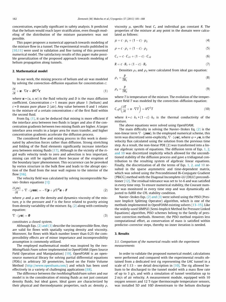
Fig. 1. Computational domain, D = 0.292 m, L = 15D, l = 5D. Temperature of theejected helium THel = 119 K, temperature of the ventilation air Tair = 292.5 K, initialpressure in the channel p0 = 0.1 MPa.

Ziemowit (M) Malecha et al. / Cryogenics 57 (2013) 181–188 183

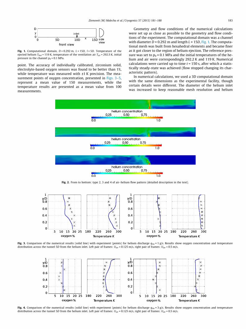
point. The accuracy of individually calibrated, zirconium solid,electrolyte-based oxygen sensors was found to be better than 1%,while temperature was measured with ±1 K precision. The mea-surement points of oxygen concentration, presented in Figs. 3–5,represent a mean value of 150 measurements, while thetemperature results are presented as a mean value from 100measurements.

Fig. 2. From to bottom: type 2, 3 and 4 of air–helium

Fig. 3. Comparison of the numerical results (solid line) with experiment (points) for hdistribution across the tunnel 5D from the helium inlet. Left pair of frames: Uair = 0.125

Fig. 4. Comparison of the numerical results (solid line) with experiment (points) for hdistribution across the tunnel 5D from the helium inlet. Left pair of frames: Uair = 0.125

Geometry and flow conditions of the numerical calculationswere set up as close as possible to the geometry and flow condi-tions of the experiment. The computational domain was a channelwith diameter D = 0.292 m and length L = 15D, Fig. 1. The computa-tional mesh was built from hexahedral elements and became fineras it got closer to the region of helium ejection. The reference pres-sure was set to p0 = 0.1 MPa and the initial temperatures of the he-lium and air were correspondingly 292.2 K and 119 K. Numericalcalculations were carried up to time t = 150 s, after which a statis-tically steady-state was achieved (flow stopped changing its char-acteristic pattern).

In numerical calculations, we used a 3D computational domainwith the same dimensions as the experimental facility, thoughcertain details were different. The diameter of the helium inletwas increased to keep reasonable mesh resolution and helium

flow pattern (detailed description in the text).

elium discharge qHe = 1 g/s. Results show oxygen concentration and temperaturem/s, right pair of frames: Uair = 0.5 m/s.

elium discharge qHe = 3 g/s. Results show oxygen concentration and temperaturem/s, right pair of frames: Uair = 0.5 m/s.

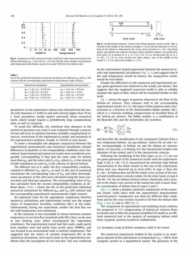
Fig. 5. Comparison of the numerical results (solid line) with experiment (points) forhelium discharge qHe = 3 g/s and Uair = 0.5 m/s. Results show oxygen concentrationand temperature distribution across the tunnel 10D from the helium inlet.

Table 1List of the performed individual numerical calculations for different qHe and Uair (leftcolumn) and the corresponding experimental measurements (right column).

Numerical calculations Experimental measurements

1. qHe = 1 g/s, Uair = 0.125 m/s qHe = 1 g/s, Uair = 0.5 m/s2. qHe = 1 g/s, Uair = 0.5 m/s qHe = 1 g/s, Uair = 2 m/s3. qHe = 3 g/s, Uair = 0.125 m/s qHe = 3 g/s, Uair = 0.5 m/s4. qHe = 3 g/s, Uair = 0.125 m/s qHe = 3 g/s, Uair = 2 m/s

Fig. 6. Computational domain. Tunnel with helium pipeline system inside. Pipe islocated in the middle of the tunnel at height y = 2.4 m and has diameter d = 0.3 m.Inlet of the helium is indicated by the arrow and is located at x = 4 m. Two blackpoints and dashed line indicate locations where detailed analysis was performed.First point (A) is located at (x, y, z) = (12.3, 3.9, 1.5) m, second point (B) at (x, y,z) = (0.1, 1.7, 1.5) m. Cross-section was taken along x axis, in the middle of thetunnel (z = 1.5 m) and at the height y = 1.7 m.

184 Ziemowit (M) Malecha et al. / Cryogenics 57 (2013) 181–188

parameters. In the experiment, helium was released from the noz-zle with diameter d = 0.003 m and with velocity higher than 70 m/s. Such parameters would require extremely dense numericalmesh, which would require a prohibitively long computationaltime, as well as resources.

To avoid this difficulty, the substitute inlet diameter in thenumerical geometry was used. It was evaluated through a processof trial-and-error to optimize between available computational re-sources, restrictions of the mathematical model, and proximity tothe experimental conditions. Finally, d = 0.0143 m was chosen.

To make a meaningful and adequate comparison between theexperimental measurements and numerical calculations, despitedifferences in diameter d, two comparability conditions were con-sidered. Experimental and numerical results were considered com-parable (corresponding) if they had the same value for heliummass flow qHe and the same ratio Uair/UHe, where Uair is the velocityof inlet ventilation air and UHe is the velocity of ejected helium.

The different size in d, under the first comparability condition,resulted in different UHe and Uair as well. In the case of numericalcalculations the corresponding value of UHe and other thermody-namic parameters at the inlet were calculated using the mass con-servation and ideal gas equations. The corresponding value of UHe

was calculated from the second comparability condition, as de-fined above. Table 1 shows the list of the performed individualnumerical calculations for different qHe and Uair (left column) andthe corresponding experimental measurements (right column).

An important issue for the appropriate comparison betweennumerical calculations and experimental results was the properchoice of temperature boundary conditions (BCs) at the walls.Unfortunately, during the experiment, neither the heat flux northe wall temperature was monitored.

In this situation, it was reasonable to choose between constanttemperature or zero heat flux (insulated walls) BCs (they can be seenas two limiting cases which encompassed the experimentconditions). The experimental tunnel had thin walls, made partlyfrom stainless steel and partly from acrylic glass (PMMA), andwas located in an environment with a constant temperature. Thissuggested that the choice of constant temperature BCs in thenumerical calculations, were much closer to the experimental con-ditions than the assumption of zero heat flux. This was confirmed

by the achievement of good agreement between the numerical re-sults and experimental calculations (Figs. 2–5) and suggests that ifthe wall temperature would be known, the comparative resultswould be even better.

Despite the differences in the numerical and experimental set-ups, good agreement was achieved in the results (see below). Thissuggests that the employed numerical model is able to reliablysimulate the types of flow, which will be examined further in thiswork.

Fig. 2. shows the types of patterns observed in the flow of thehelium–air mixture. They compare well to the correspondingexperimental results. In [10], the types of flow patterns were char-acterized as a function of the dimensionless Bakke number (Ba0),which is a criterion enabling categorization of stratified flows ofthe helium-air mixture. The Bakke number is a combination ofthe Reynolds (Re) and the Archimedes (Ar) numbers:

Ba0 ¼ Re2

ArUair

UHe¼

UairDvair

� �2

gD3qHe�qcvair qair

Uair

UHeð11Þ

and describes the stratification of one component (helium) from atwo component (helium�air) gas mixture . Indices He, air and c re-fer, correspondingly, to helium, air and the helium–air mixture,where v is viscosity, q is density, D is the characteristic length scale(diameter of the tunnel) and U is the characteristic velocity.

Following the numbering of the flow types, as in [10], we cansee good agreement of the numerical results with the experiment.Type 2 (for 2 6 Ba0 < 4) is characterized by relatively high heliumconcentration in the whole tunnel (in the case of the experiment,dense mist was observed up to level 0.9D). In type 3, flow (for4 6 Ba0 < 8) helium does not fill the whole cross-section of the tun-nel and stratification is clearly visible. On the other hand, in type 4(for Ba0 < 8), the air-helium mixture moves chaotically and is pres-ent in the whole cross-section of the tunnel but with a much smal-ler concentration of helium than in types 2 and 3.

Figs. 3–5 show a detailed, pointwise comparison of the numer-ical results (solid lines) with the experimental measurements(asterisk points). Comparison was done for different flow condi-tions and for the cross-section, located at 5D from the helium inlet(Figs. 3 and 4), and at 10D (Fig. 5).

The comparison of experimental and modeling result confirmsthe proposed in [10] categorization of helium-air mixture flowsin tunnels and verifies the proposed simplified 3D model as an effi-cient numerical tool in the analysis of emergency helium relieffrom cryogenic systems located in confinements.

3.2. Exemplary study of helium emergency relief to the tunnel

The numerical experiment studied in this section is an emer-gency ejection of the cold helium, at temperature THe = 100 K, fromcryogenic system to a hypothetical tunnel. The geometry of the

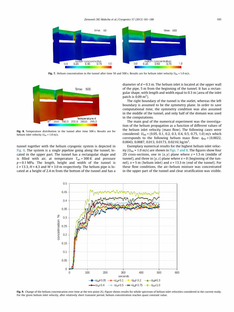
Fig. 7. Helium concentration in the tunnel after time 50 and 500 s. Results are for helium inlet velocity UHe = 1.0 m/s.

Fig. 8. Temperature distribution in the tunnel after time 500 s. Results are forhelium inlet velocity UHe = 1.0 m/s.

Ziemowit (M) Malecha et al. / Cryogenics 57 (2013) 181–188 185

tunnel together with the helium cryogenic system is depicted inFig. 6. The system is a single pipeline going along the tunnel, lo-cated in the upper part. The tunnel has a rectangular shape andis filled with air, at temperature Tair = 300 K and pressurep = 0.1 MPa. The length, height and width of the tunnel isL = 13.3, H = 4.3 and W = 3.0 m respectively. The helium pipe is lo-cated at a height of 2.4 m from the bottom of the tunnel and has a

Fig. 9. Change of the helium concentration over time at the test point (A). Figure shows rFor the given helium inlet velocity, after relatively short transient period, helium conce

diameter of d = 0.3 m. The helium inlet is located at the upper wallof the pipe, 5 m from the beginning of the tunnel. It has a rectan-gular shape, with length and width equal to 0.3 m (area of the inletpatch is 0.09 m2).

The right boundary of the tunnel is the outlet, whereas the leftboundary is assumed to be the symmetry plane. In order to savecomputational time, the symmetry condition was also assumedin the middle of the tunnel, and only half of the domain was usedin the computations.

The main goal of the numerical experiment was the investiga-tion of the helium propagation as a function of different values ofthe helium inlet velocity (mass flow). The following cases wereconsidered: UHe = (0.05, 0.1, 0.2, 0.3, 0.4, 0.5, 0.75, 1.0) m/s whichcorresponds to the following helium mass flow: qHe = (0.0022,0.0043, 0.0087, 0.013, 0.0173, 0.0216) kg/m3.

Exemplary numerical results for the highest helium inlet veloc-ity (UHe = 1.0 m/s) are shown in Figs. 7 and 8. The figures show four2D cross-sections, one in (x, y) plane where z = 1.5 m (middle oftunnel), and three in (y, z) plane where x = 0 (beginning of the tun-nel), x = 5 m (helium inlet) and x = 13.3 m (end of the tunnel). Forthese flow conditions, the air–helium mixture was concentratedin the upper part of the tunnel and clear stratification was visible.

esults for whole spectrum of helium inlet velocities considered in the current study.ntration reaches quasi constant value.

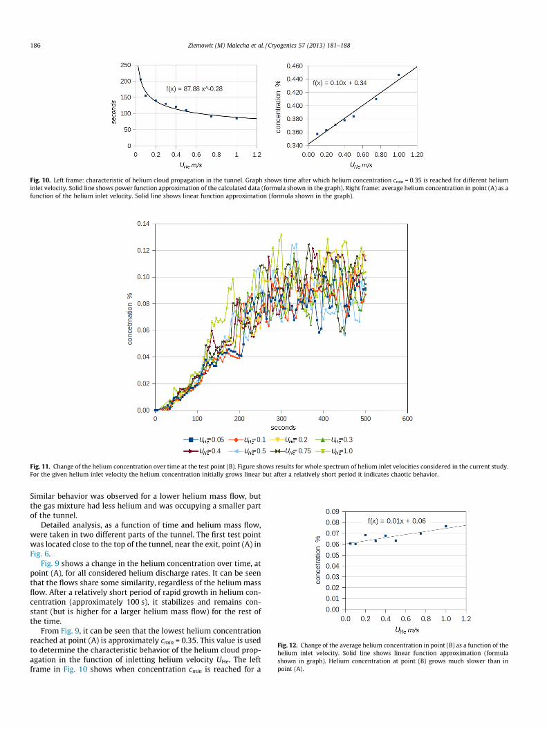
Fig. 10. Left frame: characteristic of helium cloud propagation in the tunnel. Graph shows time after which helium concentration cmin = 0.35 is reached for different heliuminlet velocity. Solid line shows power function approximation of the calculated data (formula shown in the graph). Right frame: average helium concentration in point (A) as afunction of the helium inlet velocity. Solid line shows linear function approximation (formula shown in the graph).

Fig. 11. Change of the helium concentration over time at the test point (B). Figure shows results for whole spectrum of helium inlet velocities considered in the current study.For the given helium inlet velocity the helium concentration initially grows linear but after a relatively short period it indicates chaotic behavior.

Fig. 12. Change of the average helium concentration in point (B) as a function of thehelium inlet velocity. Solid line shows linear function approximation (formulashown in graph). Helium concentration at point (B) grows much slower than inpoint (A).

186 Ziemowit (M) Malecha et al. / Cryogenics 57 (2013) 181–188

Similar behavior was observed for a lower helium mass flow, butthe gas mixture had less helium and was occupying a smaller partof the tunnel.

Detailed analysis, as a function of time and helium mass flow,were taken in two different parts of the tunnel. The first test pointwas located close to the top of the tunnel, near the exit, point (A) inFig. 6.

Fig. 9 shows a change in the helium concentration over time, atpoint (A), for all considered helium discharge rates. It can be seenthat the flows share some similarity, regardless of the helium massflow. After a relatively short period of rapid growth in helium con-centration (approximately 100 s), it stabilizes and remains con-stant (but is higher for a larger helium mass flow) for the rest ofthe time.

From Fig. 9, it can be seen that the lowest helium concentrationreached at point (A) is approximately cmin = 0.35. This value is usedto determine the characteristic behavior of the helium cloud prop-agation in the function of inletting helium velocity UHe. The leftframe in Fig. 10 shows when concentration cmin is reached for a

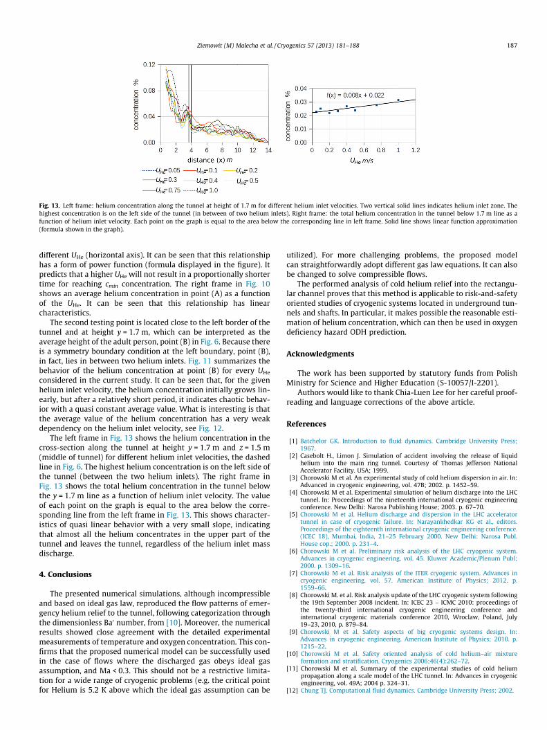
Fig. 13. Left frame: helium concentration along the tunnel at height of 1.7 m for different helium inlet velocities. Two vertical solid lines indicates helium inlet zone. Thehighest concentration is on the left side of the tunnel (in between of two helium inlets). Right frame: the total helium concentration in the tunnel below 1.7 m line as afunction of helium inlet velocity. Each point on the graph is equal to the area below the corresponding line in left frame. Solid line shows linear function approximation(formula shown in the graph).

Ziemowit (M) Malecha et al. / Cryogenics 57 (2013) 181–188 187

different UHe (horizontal axis). It can be seen that this relationshiphas a form of power function (formula displayed in the figure). Itpredicts that a higher UHe will not result in a proportionally shortertime for reaching cmin concentration. The right frame in Fig. 10shows an average helium concentration in point (A) as a functionof the UHe. It can be seen that this relationship has linearcharacteristics.

The second testing point is located close to the left border of thetunnel and at height y = 1.7 m, which can be interpreted as theaverage height of the adult person, point (B) in Fig. 6. Because thereis a symmetry boundary condition at the left boundary, point (B),in fact, lies in between two helium inlets. Fig. 11 summarizes thebehavior of the helium concentration at point (B) for every UHe

considered in the current study. It can be seen that, for the givenhelium inlet velocity, the helium concentration initially grows lin-early, but after a relatively short period, it indicates chaotic behav-ior with a quasi constant average value. What is interesting is thatthe average value of the helium concentration has a very weakdependency on the helium inlet velocity, see Fig. 12.

The left frame in Fig. 13 shows the helium concentration in thecross-section along the tunnel at height y = 1.7 m and z = 1.5 m(middle of tunnel) for different helium inlet velocities, the dashedline in Fig. 6. The highest helium concentration is on the left side ofthe tunnel (between the two helium inlets). The right frame inFig. 13 shows the total helium concentration in the tunnel belowthe y = 1.7 m line as a function of helium inlet velocity. The valueof each point on the graph is equal to the area below the corre-sponding line from the left frame in Fig. 13. This shows character-istics of quasi linear behavior with a very small slope, indicatingthat almost all the helium concentrates in the upper part of thetunnel and leaves the tunnel, regardless of the helium inlet massdischarge.

4. Conclusions

The presented numerical simulations, although incompressibleand based on ideal gas law, reproduced the flow patterns of emer-gency helium relief to the tunnel, following categorization throughthe dimensionless Ba0 number, from [10]. Moreover, the numericalresults showed close agreement with the detailed experimentalmeasurements of temperature and oxygen concentration. This con-firms that the proposed numerical model can be successfully usedin the case of flows where the discharged gas obeys ideal gasassumption, and Ma < 0.3. This should not be a restrictive limita-tion for a wide range of cryogenic problems (e.g. the critical pointfor Helium is 5.2 K above which the ideal gas assumption can be

utilized). For more challenging problems, the proposed modelcan straightforwardly adopt different gas law equations. It can alsobe changed to solve compressible flows.

The performed analysis of cold helium relief into the rectangu-lar channel proves that this method is applicable to risk-and-safetyoriented studies of cryogenic systems located in underground tun-nels and shafts. In particular, it makes possible the reasonable esti-mation of helium concentration, which can then be used in oxygendeficiency hazard ODH prediction.

Acknowledgments

The work has been supported by statutory funds from PolishMinistry for Science and Higher Education (S-10057/I-2201).

Authors would like to thank Chia-Luen Lee for her careful proof-reading and language corrections of the above article.

References

[1] Batchelor GK. Introduction to fluid dynamics. Cambridge University Press;1967.

[2] Casebolt H., Limon J. Simulation of accident involving the release of liquidhelium into the main ring tunnel. Courtesy of Thomas Jefferson NationalAccelerator Facility. USA; 1999.

[3] Chorowski M et al. An experimental study of cold helium dispersion in air. In:Advanced in cryogenic engineering, vol. 47B; 2002. p. 1452–59.

[4] Chorowski M et al. Experimental simulation of helium discharge into the LHCtunnel. In: Proceedings of the nineteenth international cryogenic engineeringconference. New Delhi: Narosa Publishing House; 2003. p. 67–70.

[5] Chorowski M et al. Helium discharge and dispersion in the LHC acceleratortunnel in case of cryogenic failure. In: Narayankhedkar KG et al., editors.Proceedings of the eighteenth international cryogenic engineering conference.(ICEC 18), Mumbai, India, 21–25 February 2000. New Delhi: Narosa Publ.House cop.; 2000. p. 231–4.

[6] Chorowski M et al. Preliminary risk analysis of the LHC cryogenic system.Advances in cryogenic engineering, vol. 45. Kluwer Academic/Plenum Publ;2000. p. 1309–16.

[7] Chorowski M et al. Risk analysis of the ITER cryogenic system. Advances incryogenic engineering, vol. 57. American Institute of Physics; 2012. p.1559–66.

[8] Chorowski M. et al. Risk analysis update of the LHC cryogenic system followingthe 19th September 2008 incident. In: ICEC 23 – ICMC 2010: proceedings ofthe twenty-third international cryogenic engineering conference andinternational cryogenic materials conference 2010, Wroclaw, Poland, July19–23, 2010, p. 879–84.

[9] Chorowski M et al. Safety aspects of big cryogenic systems design. In:Advances in cryogenic engineering. American Institute of Physics; 2010. p.1215–22.

[10] Chorowski M et al. Safety oriented analysis of cold helium–air mixtureformation and stratification. Cryogenics 2006;46(4):262–72.

[11] Chorowski M et al. Summary of the experimental studies of cold heliumpropagation along a scale model of the LHC tunnel. In: Advances in cryogenicengineering, vol. 49A; 2004 p. 324–31.

[12] Chung TJ. Computational fluid dynamics. Cambridge University Press; 2002.

188 Ziemowit (M) Malecha et al. / Cryogenics 57 (2013) 181–188

[13] Ferziger J, Peric M. Computational methods for fluiddynamics. Berlin: Springer; 1999.

[14] Issa R et al. The computation of compressible and incompressible recirculatingflows by a non-iterative implicit scheme. J Comput Phys 1986;62:66–82.

[15] Issa R. Solution of implicitly discretized fluid flow equations by operator-splitting. J Comput Phys 1986;62:40–65.

[16] Kudela H, Malecha ZM. Eruption of a boundary layer induced by a 2D vortexpatch. Fluid Dyn Res 2009;41(5):055502.

[17] Malecha K et al. Serpentine microfluidic mixer made in LTCC. Sens Actuators B2009;143:400–13.

[18] Malecha Z et al. Gpu-based simulation of 3d blood flow in abdominal aortausing OpenFOAM. Arch Mech 2011;63:137–61.

[19] OpenFOAM. The open source CFD toolbox user guide. Free SoftwareFoundation, Inc.; 2009.

[20] Rode CH et al. Injector helium spill test. Courtesy of Thomas Jefferson NationalAkccelerator Facility. USA; 1991.

[21] Soyars WM, Schiller JL. Open channel helium flow during rapture event.Advances in cryogenic engineering, vol. 47 B. New York: Melville; 2002. p.1776–83.