Abstract This paper describes the influence of geometrical parameters on the hydrofoil performance in non-cavitating and cavitating flows. The
two-phase incompressible Navier-Stokes solver is used to compute the hydrofoil performance in two operating conditions. The new hy-drofoil useful for performance improvement is obtained through the optimization design with RSM and the application of nose-drooping geometry. In the optimization design with the response surface model between hydrofoil performance and hydrofoil geometry, it is ob-served that the design concept of maximum lift-to-drag ratio is appropriate for the improvement of hydrofoil performance. The applica-tion of nose-drooping design concept results in the increase of hydrofoil performance in non-cavitating and cavitating flows.
Cavitation is usually found in the fluid flows where the lo-cal pressure drops below the vapor pressure of the liquid, causing the liquid evaporation and the generation of vapor bubbles in the low pressure region. A number of different approaches have been developed to deal with the equation of state for cavitating flows [1, 2]. Recently, the comparison analysis with various mass transfer models [3] and the appli-cation of a large eddy simulation (LES) scheme [4, 5] have become an object of attention in the field of cavitating flow. Furthermore, the unsteady dynamic characteristics of cavitat-ing flow such as the water flow over the oscillating hydrofoil [6] have been a subject of interest.
The existence of cavitation is often undesired, because it can degrade the performance of fluid machinery, produce undesirable noise, lead to the physical damage of the device, and affect structural integrity. Therefore, many researches have been carried out to account for cavitation effects and to minimize cavitation, which can be of significant help during the optimization design stage of fluid machinery [7]. From this point of view, this present study is focused on examining the effect of hydrofoil geometry on cavitating flow, and suggesting the new design concept to reduce the cavitation effect.
2. Flow solver
The governing equations are the gas-liquid two-phase Na-vier-Stokes equations with a volume fraction transport equa-tion to account for cavitating flow and are written as follows [8]:
( ) ⎟⎟⎠
⎞⎜⎜⎝
⎛−+=
∂∂
+∂∂
⎟⎟⎠
⎞⎜⎜⎝
⎛ −+
vlj
j
m
mmxup
ρρτβρ111
&&
( ) ( ) ( )
j
ij
ijim
jimim xx
puux
uut ∂
∂+
∂∂
−=∂∂
+∂∂
+∂∂ τ
ρρτ
ρˆ
(1)
( ) ( ) ⎟⎟⎠
⎞⎜⎜⎝
⎛+=
∂∂
+∂∂
+∂∂
⎟⎟⎠
⎞⎜⎜⎝
⎛+
∂∂ −+
ljl
j
l
m
ll mmux
pt ρ
ατα
τβραα 1
&&
where the mixture density, mρ is defined as
( )1 .m l l v lρ ρ α ρ α= + − (2) In Eq. (1), lρ is the liquid density, vρ is the vapor den-
sity, lα is the liquid volume fraction, β is the pseudo-compressibility parameter (here, 800β = ), τ is the pseudo-time, t is the physical time, ( ), ,jx x y z= are the Cartesian coordinates, ( ), ,ju u v w= are the Cartesian components of the velocity, p is the static pressure, and ijτ is composed of the molecular and Reynolds stresses defined as
( ),ˆ 2 /3ij m l ij kk ij ijS Sτ μ δ τ= − +
( ),2 / 3 2 / 3ij m t ij kk ij m ijS S kτ μ δ ρ δ= − −
2536 H. Sun / Journal of Mechanical Science and Technology 26 (8) (2012) 2535~2545
12
jiij
j i
uuSx x
⎛ ⎞∂∂= +⎜ ⎟⎜ ⎟∂ ∂⎝ ⎠
(3)
where ,m lμ is the laminar mixture viscosity, ,m tμ is the turbulent eddy mixture viscosity, ijδ is the Kronecker delta, and ijS is the mean strain-rate tensor. The mass transfer rates from the vapor to the liquid and from the liquid to the vapor are denoted by m+ and m− , respectively [8]. A simplified form of the Ginzburg-Landau potential [9, 10] is employed in m+ , and m− is modeled as being proportional to the liquid volume fraction and the amount by which the pressure is be-low the vapor pressure, pv.
( )2
min 0,
1/ 2dest v l v
l
C p pm
u t
ρ α
ρ−
∞ ∞
−⎡ ⎤⎣ ⎦=&
( )2 1prod v l lCm
tρ α α+
∞
−=& (4)
where destC and prodC are the empirical constants (here,
100destC = , 100prodC = ), u∞ is the mean flow velocity, and t∞ is the mean flow time scale.
In this work, the k ε− turbulence model is evaluated to take the turbulence effect into account [11]. The standard k ε− model is transformed into the k ω− formulation using the relation of 0.09 ,kε ω= and the transformed k ε− model has the transport equations of the turbulent kinetic energy, k and the specific dissipation rate, ω and is written as follows:
( ) ( )*, ,
m im j ij m m l k m t
j j j j
k u kku kt x x x x
ρ ρ τ β ρ ω μ σ μ⎡ ⎤∂ ∂ ∂ ∂ ∂
+ = − + +⎢ ⎥∂ ∂ ∂ ∂ ∂⎢ ⎥⎣ ⎦
( ) ** 2
,
m im j ij m
j m t j
uut x x
ρ ω γρ ω τ β ρ ων
∂ ∂ ∂+ = −
∂ ∂ ∂
( ), ,12m l m t m
j j j j
kx x x xω ω
ω ωμ σ μ ρ σω
⎡ ⎤∂ ∂ ∂ ∂+ + +⎢ ⎥∂ ∂ ∂ ∂⎢ ⎥⎣ ⎦
(5)
where ( ),2 / 3ij m t ij kk ijS Sτ μ δ= − , ,m tν is the turbulent mixture kinematic viscosity, and the constants of the transformed k ε− model are given below [12]:
** *
** * 2 *
1.0 , 0.856 , 0.0828 , 0.09 , 0.41
/ / .k ω
ω
σ σ β β κ
γ β β σ κ β
= = = = =
= −
The governing equations are solved with a finite volume
method. For the calculation of the residual, the convective terms are differenced using the third-order upwind differenc-ing scheme with MUSCL approach [13], and the viscous terms are differenced using second-order central difference. For temporal integration, LU-SGS scheme is adopted to effi-ciently solve the governing equations [14].
The turbulent cavitating flow over the CAV2003 hydrofoil
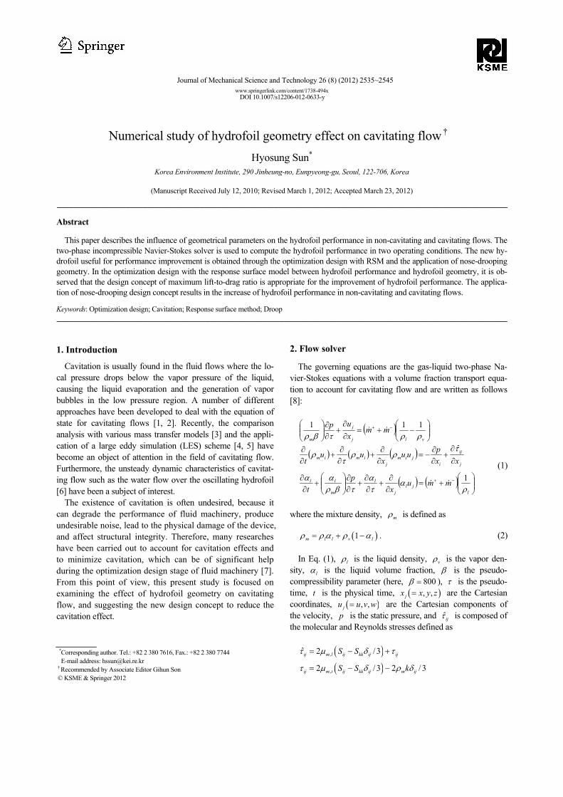
[15] operated at the angle of attack, α of 7° and the Rey-nolds number, Re of 5.9× 10⁵ is computed to validate the numerical code [16]. The grid sensitivity studies in the cavita-tion number (Eq. (6)), 3.5σ = are performed with an O-type grid system, in which the grid sizes are 65× 43, 129× 85, 257× 85, 257× 169 in streamwise and perpendicular direc-tions, respectively.
21/ 2vp p
uσ
ρ∞
∞ ∞
−= (6)
In Eq. (6), vp means the vapor pressure and , ,p uρ∞ ∞ ∞
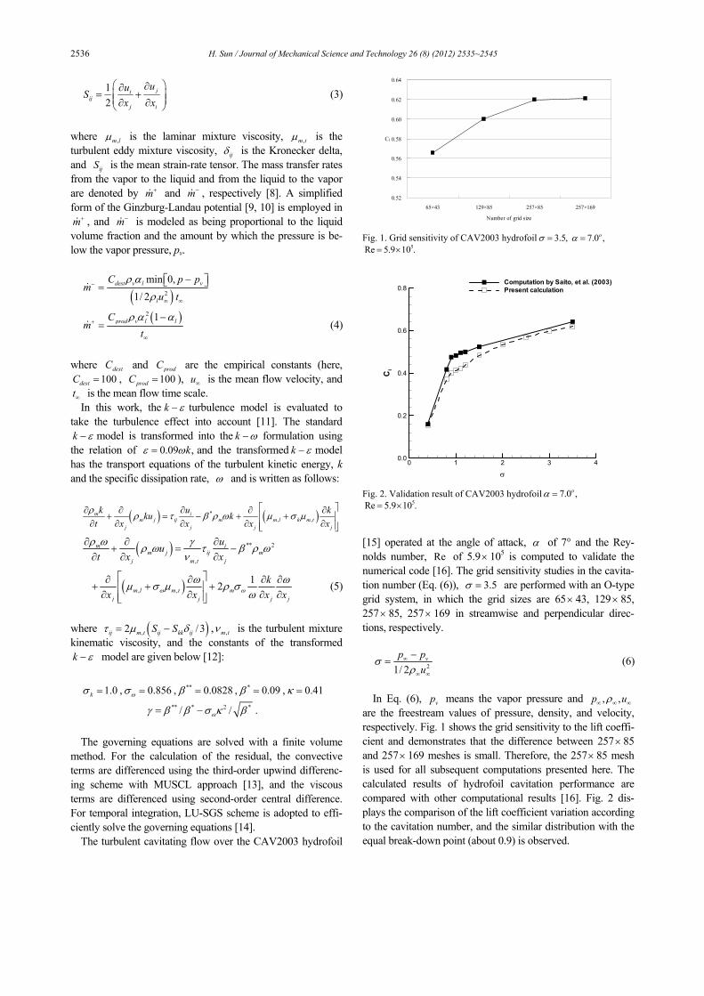
are the freestream values of pressure, density, and velocity, respectively. Fig. 1 shows the grid sensitivity to the lift coeffi-cient and demonstrates that the difference between 257× 85 and 257× 169 meshes is small. Therefore, the 257× 85 mesh is used for all subsequent computations presented here. The calculated results of hydrofoil cavitation performance are compared with other computational results [16]. Fig. 2 dis-plays the comparison of the lift coefficient variation according to the cavitation number, and the similar distribution with the equal break-down point (about 0.9) is observed.
0.8Computation by Saito, et al. (2003)Present calculation
Fig. 2. Validation result of CAV2003 hydrofoil 7.0 ,oα =
5Re 5.9 10 .= ×
H. Sun / Journal of Mechanical Science and Technology 26 (8) (2012) 2535~2545 2537
3. Results and discussion
The two approach methods are proposed to investigate the effect of a hydrofoil section on cavitating flow. One is the hydrofoil optimization design based on response surface method (hereafter, RSM), and the other is the hydrofoil design concept with the drooped leading edge which is originated to reduce the dynamic stall phenomenon of a helicopter rotor [17-19]. The turbulent non-cavitating ( )/ 2 9σ α = and cavi-tating ( )/ 2 2σ α = flows over the NACA0015 hydrofoil operated at the angle of attack, α of 9° and the Reynolds number, Re of 1.2× 10⁶ are applied to carry out the two hydrofoil design works [20]. The composite parameter,
/ 2σ α connected with the cavitation number, σ and the angle of attack, α is used to express cavitating flow property.
3.1 Optimization design with RSM
RSM is the collection of the statistical and mathematical techniques useful for developing and improving the optimiza-tion process [21], and builds a response model by calculating the data points with experimental design theory to prescribe the response of the system with independent variables. The relationship can be written in a general form as follows:
( )1 2, , ,vny F x x x ε= +L (7)
where y is the response variable, xi are the design variables, and ε represents the total error which is often assumed to have a normal distribution with zero mean.
The response surface model, F is usually assumed as a second-order polynomial, which can be written for vn design variables as follows:
( )
01
, 1, ,v
pi i ij i j s
i i j n
y c c x c x x p n≤ ≤ ≤
= + + =∑ ∑ L (8)
where ( )py is the dependent variable of the response surface model, 0 , ,i ijc c c are the regression coefficients, and sn is the number of observations. The above normal equations are expressed in a matrix form and the method of least-squares is typically used to estimate the regression coefficients in a mul-tiple linear regression model.
y Xc=r r
( ) 1T Tc X X X y−
=r r (9)
where y
r is the response vector, X is the s rcn n× matrix, rcn is the number of regression coefficients, and c
r is the vector of regression coefficients.
As a selection technique of data points, the 3-level factorial design with the D-optimal condition is applied. The 3-level factorial design is created by specifying lower bound, mid-point, and upper bound [-1, 0, 1] for each design variable.
According to the D-optimal criterion, the selected points are those that maximize the determinant, TX X . The data-points set that maximizes TX X is the set of data points that mini-mizes the maximum variance of any predicted value from the regression model, which also means the set of data points that minimizes the variance of regression coefficients.
The analysis of variance and the regression analysis are ap-plied to estimate the regression coefficients in the quadratic polynomial model, and also yield the measure of uncertainty in the coefficients. The regression model expresses the rela-tionship between responses and independent variables, which partially explains observations through fitted values. The rela-tionship between the response and the approximation model can be represented as follows:
( )ˆ
i i iy f x ε= +
( ) ( ) 20 vari iE andε ε δ= = (10)
where ( )ˆ
if x is the response surface model and the random variables, iε are the errors that create the scatter around the linear relationship. It is assumed that these errors are mutually independent and normally distributed with zero mean and variance, 2δ . The variation of the responses, iy and the fitted values, ˆiy about the mean, y can be measured in terms of total sum of squares (SSTO), regression sum of squares (SSR), and error sum of squares (SSE).
( ) ( )22
1 1 1
ˆ, ,s s sn n n
i i ii i i
SSTO y y SSR y y SSE ε= = =
= − = − =∑ ∑ ∑
SSTO SSR SSE= + (11) One of the important statistical parameters is the coefficient
of determination, 2R which provides the summary statistic that measures how well the regression equation fits the data.
2 21 , 0 1SSR SSER R
SSTO SSTO= = − ≤ ≤ (12)
In 2R = 0, the regression model explains none of the varia-
tion in response values. On the other hand, 2R = 1 means that all sn observations lie on the fitted regression line and all of the variations are explained by the linear relationship with explanatory variables. However, a large value of 2R doesn’t necessarily imply that the regression model is good one. Add-ing a variable to the model will always increase 2R , regard-less of whether the additional variable is statistically signifi-cant or not. Because 2R always increases as the new terms are added to the model, the adjusted - 2R statistic parameter,
2adjR defined below is frequently used.
( )( ) ( )2 2/ 11 1 1
/ 1s rc s
adjs s rc
SSE n n nR RSSTO n n n
⎛ ⎞− −= − = − −⎜ ⎟⎜ ⎟− −⎝ ⎠
(13)
2538 H. Sun / Journal of Mechanical Science and Technology 26 (8) (2012) 2535~2545
In general, the adjusted - 2R statistic doesn’t always in-crease as the new variables are added to the model. In fact, if the unnecessary terms are added, the value of 2
adjR often de-creases.
It is important to determine the value of each regression variable in the regression model, because the model may be effective with the inclusion of additional variables or with the deletion of the variables already in the model. The test statistic (hereafter, t-statistic) for testing the significance of any indi-vidual regression coefficient is
j
2
ct , 1, ,
ˆ rc
jj
j nCσ
= = L (14)
where 2σ is the estimation of variance and jjC is the di-agonal element of ( ) 1TX X
− corresponding to jc .
For the low cavitation design using RSM, a NACA 0015 hydrofoil geometry is modified adding the linear combination of the shape functions, kf and the weighting coefficients,
kw as follows [22]:
1
vn
base k kk
y y w f=
= + ∑
( ) ( ) ( )( )
3 ln 0.5sin ,
lne k
kk
f x e kx
π⎡ ⎤= =⎣ ⎦ (15)
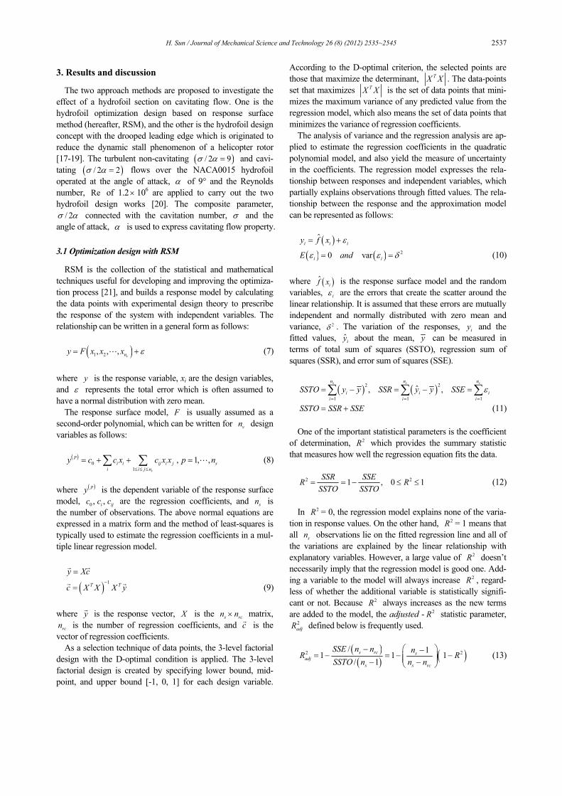
where x, y are the hydrofoil coordinates, base means the base hydrofoil, and xk represents the location of the maximum height of the base sinusoidal function. The six design variables are applied on both upper and lower sides of a NACA 0015 hydrofoil (Fig. 3). The 57 numerical simulations and the 28 regression coefficients are used to construct the quadratic re-sponse surface model.
The fitting quality about the hydrofoil lift and drag coeffi-cients in non-cavitating and cavitating flows is examined to estimate the accuracy of the response surface model (Table 1). It is observed that the hydrofoil performance depending on the change of a hydrofoil shape can be accurately predicted with the quadratic model. The t-statistic values are calculated to
estimate the importance of design variables on hydrofoil per-formance prediction in Fig. 4. The design variable of a higher t-statistic value has a more dominant effect on the response surface model. The 1x design variable for modifying the front part close to the leading edge of the hydrofoil upper sur-face is regarded as the dominant term in the hydrofoil per-formance of two operating conditions, and the t-statistic value distribution of the lift coefficient in cavitating flow shows the importance of hydrofoil lower surface variation ( 4 6x x− de-sign variables) as a countermeasure of the lift coefficient de-crease on account of the cavitation phenomenon at the hydro-foil upper surface.
Because RSM enables the designer to modify objective functions and constraints easily during the optimization proc-ess, it is needed to examine the effect of various objective functions and constraints on the designed hydrofoil shape and performance. Therefore, two kinds of design problems includ-ing hydrofoil lift and drag coefficients are applied in Table 2. According to the comparison of the hydrofoil performance by two kinds of design conditions in Table 3, the design result of Case 2 shows a higher value of the lift-to-drag ratio due to the lift coefficient increase and the drag coefficient decrease. In non-cavitating flow, the increase of the upper side and the
x / c
y/c
0 0.25 0.5 0.75 1-0.01
-0.005
0
0.005
0.01
x1x2x3x4x5x6
Fig. 3. Shape function distribution.
Table 1. Fitting quality in hydrofoil design, 69.0 , Re 1.2 10 .oα = = ×
Non-cavitating condition
( )/ 2 9σ α = Cavitating condition
( )/ 2 2σ α =
2R 2adjR 2R
2adjR
lC 1.000 1.000 1.000 1.000
dC 1.000 1.000 1.000 1.000
(a) Non-cavitating flow, / 2 9σ α =
(b) Cavitating flow, / 2 2σ α =
Fig. 4. Comparison of t-statistic values, 69.0 , Re 1.2 10 .oα = = ×
H. Sun / Journal of Mechanical Science and Technology 26 (8) (2012) 2535~2545 2539
Table 3. Comparison of hydrofoil performance 69.0 , Re 1.2 10 .oα = = ×
Non-cavitating condition
( )/ 2 9σ α = Cavitating condition
( )/ 2 2σ α =
lC dC dl CC / lC dC dl CC /
Base 0.9208 0.0407 22.6258 0.3708 0.1072 3.4578
Case 1 0.9765 0.0333 29.3263 0.3719 0.0987 3.7677
Case 2 1.0286 0.0345 29.8436 0.4282 0.1019 4.2021
Table 2. Objective function and constraint for optimization process.
(d) Pressure contour (left) and streamlines (right) of Case 2 hydrofoil
Fig. 5. Comparison of hydrofoil geometry and performance in non-cavitating flow, 6/ 2 9, 9.0 , Re 1.2 10 .oσ α α= = = ×
2540 H. Sun / Journal of Mechanical Science and Technology 26 (8) (2012) 2535~2545
decrease of the lower side in the Case 2 hydrofoil geometry (Fig. 5(a)) raise the change of the pressure distribution (Fig. 5(b)), which results in the improvement of hydrofoil perform-ance. In cavitating flow, the variation of the hydrofoil lower surface geometry (Fig. 6(a)) leads to the augmentation of hy-drofoil performance (Fig. 6(b)), which is seen in the t-statistic value distribution of cavitating flow (Fig. 4(b)). The variation of the hydrofoil upper surface (Fig. 6(a)) changes the size and shape of hydrofoil cavitation (Fig. 6(c)), which results in the decrease of the flow recirculation (Fig. 6(d)-6(e)).
3.2 Design concept with drooped leading edge
The nose-drooping airfoil geometry concept for dynamic stall control has been approached by drooping the forward portion of an airfoil at a high angle of attack so that the flow can easily pass around the leading edge. In order to investigate the effect of a nose-drooping hydrofoil on non-cavitating and cavitating flows, the computation of the non-cavitating and cavitating hydrofoil performance about several drooped hy-drofoil configurations is made with the center of rotation, xcr/c
x / c
y/c
0 0.25 0.5 0.75 1-0.1
-0.05
0
0.05
0.1
NACA 0015Case 2
x / c
-Cp
0 0.25 0.5 0.75 1-1.5
-1.0
-0.5
0.0
0.5
1.0NACA 0015Case 2
x / c
y/c
0 0.5-0.5
-0.25
0
0.25
0.5
(a) Hydrofoil geometry (b) Pressure coefficient (c) Size and shape of hydrofoil cavitation (solid lines: NACA 0015, thick solid and dash lines: Case 2)
(e) Pressure contour (left), streamlines (middle), and liquid volume fraction contour (right) of Case 2 hydrofoil Fig. 6. Comparison of hydrofoil geometry and performance in cavitating flow, 6/ 2 2, 9.0 , Re 1.2 10 .oσ α α= = = ×
H. Sun / Journal of Mechanical Science and Technology 26 (8) (2012) 2535~2545 2541
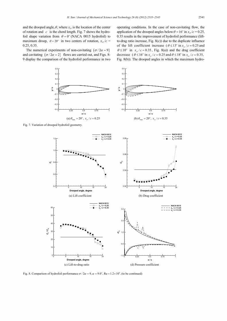
and the drooped angle, ,θ where xcr is the location of the center of rotation and c is the chord length. Fig. 7 shows the hydro-foil shape variation from 0oθ = (NACA 0015 hydrofoil) to maximum droop, 20oθ = in two centers of rotation, xcr /c = 0.25, 0.35.
The numerical experiments of non-cavitating ( )/ 2 9σ α = and cavitating ( )/ 2 2σ α = flows are carried out, and Figs. 8-9 display the comparison of the hydrofoil performance in two
operating conditions. In the case of non-cavitating flow, the application of the drooped angles below 16oθ = in xcr /c = 0.25, 0.35 results in the improvement of hydrofoil performance (lift-to-drag ratio increase, Fig. 8(c)) due to the duplicate influence of the lift coefficient increase ( 13oθ ≤ in / 0.25crx c = and
10oθ ≤ in / 0.35crx c = , Fig. 8(a)) and the drag coefficient decrease ( 16oθ ≤ in / 0.25crx c = and 18oθ ≤ in / 0.35,crx c = Fig. 8(b)). The drooped angles in which the maximum hydro-
x / c
y/c
0 0.25 0.5 0.75 1-0.4
-0.3
-0.2
-0.1
0
0.1
0.2
0.3
0.4
x / c
y/c
0 0.25 0.5 0.75 1-0.4
-0.3
-0.2
-0.1
0
0.1
0.2
0.3
0.4
(a) max 20 , / 0.25o
crx cθ = = (b) max 20 , / 0.35ocrx cθ = =
Fig. 7. Variation of drooped hydrofoil geometry.
Drooped angle, degree
Cl
0 5 10 15 200.4
0.6
0.8
1.0
1.2
NACA 0015xcr / c = 0.25xcr / c = 0.35
Drooped angle, degree
Cd
0 5 10 15 200.02
0.04
0.06
0.08
NACA 0015xcr / c = 0.25xcr / c = 0.35
(a) Lift coefficient (b) Drag coefficient
Drooped angle, degree
Cl/Cd
0 5 10 15 200
10
20
30
40
50
60
NACA 0015xcr / c = 0.25xcr / c = 0.35
x / c
-Cp
0 0.25 0.5 0.75 1-1.0
0.0
1.0
2.0
3.0
NACA 0015xcr / c = 0.25xcr / c = 0.35
(c) Lift-to-drag ratio (d) Pressure coefficient
Fig. 8. Comparison of hydrofoil performance 6/ 2 9, 9.0 , Re 1.2 10 .oσ α α= = = × (to be continued)
2542 H. Sun / Journal of Mechanical Science and Technology 26 (8) (2012) 2535~2545
foil performance can be obtained are 5o in / 0.25crx c = and 4o in / 0.35crx c = (Fig. 8(c)). The comparison analysis of the pressure distribution in the application of 5oθ = (Fig. 8(d)) shows the suction pressure reduction at the leading edge and the irregular pattern in the center of rotation due to nose-drooping effect. In cavitating flow analysis, the lift coefficient distribution indicates better characteristics in the drooped an-gles below 13oθ = (Fig. 9(a)), and the drag coefficient distri-bution exhibits lower values in the whole region (Fig. 9(b)). The augmentation of the hydrofoil lift-to-drag ratio is obtained in the drooped angles below 16oθ = (Fig. 9(c)), and the posi-
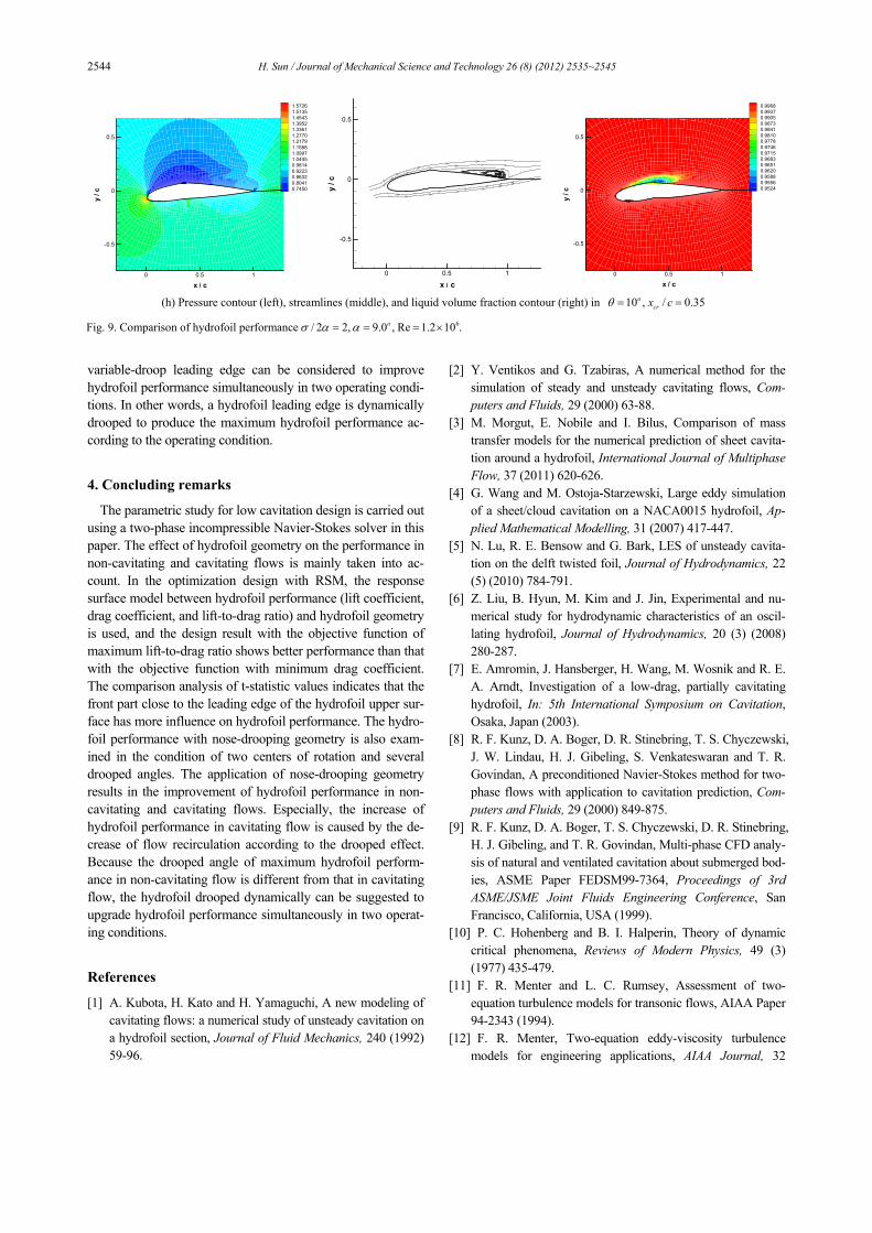
tions where the hydrofoil lift-to-drag ratio is maximum are 10o in / 0.25crx c = and 12o in / 0.35crx c = . The distribution of the pressure coefficient in the application of 10oθ = shows the formation range of sheet cavitation in the hydrofoil upper surface (Fig. 9(d)). The application of the drooped hy-drofoil gives rise to the change of the cavitation size, shape, and location (Fig. 9(e)), which results in the decrease of the flow recirculation (Fig. 9(f)-9(h)). From the above results, the nose-drooping concept exhibits the possibility of improving the hydrofoil performance in the circumstances of non-cavitating and cavitating flows, and the design concept of a
(g) Pressure contour (left), streamlines (middle), and liquid volume fraction contour (right) in 10 , / 0.25ocrx cθ = =
Fig. 9. Comparison of hydrofoil performance 6/ 2 2, 9.0 , Re 1.2 10 .oσ α α= = = × (to be continued)
2544 H. Sun / Journal of Mechanical Science and Technology 26 (8) (2012) 2535~2545
variable-droop leading edge can be considered to improve hydrofoil performance simultaneously in two operating condi-tions. In other words, a hydrofoil leading edge is dynamically drooped to produce the maximum hydrofoil performance ac-cording to the operating condition.
4. Concluding remarks
The parametric study for low cavitation design is carried out using a two-phase incompressible Navier-Stokes solver in this paper. The effect of hydrofoil geometry on the performance in non-cavitating and cavitating flows is mainly taken into ac-count. In the optimization design with RSM, the response surface model between hydrofoil performance (lift coefficient, drag coefficient, and lift-to-drag ratio) and hydrofoil geometry is used, and the design result with the objective function of maximum lift-to-drag ratio shows better performance than that with the objective function with minimum drag coefficient. The comparison analysis of t-statistic values indicates that the front part close to the leading edge of the hydrofoil upper sur-face has more influence on hydrofoil performance. The hydro-foil performance with nose-drooping geometry is also exam-ined in the condition of two centers of rotation and several drooped angles. The application of nose-drooping geometry results in the improvement of hydrofoil performance in non-cavitating and cavitating flows. Especially, the increase of hydrofoil performance in cavitating flow is caused by the de-crease of flow recirculation according to the drooped effect. Because the drooped angle of maximum hydrofoil perform-ance in non-cavitating flow is different from that in cavitating flow, the hydrofoil drooped dynamically can be suggested to upgrade hydrofoil performance simultaneously in two operat-ing conditions.
References
[1] A. Kubota, H. Kato and H. Yamaguchi, A new modeling of cavitating flows: a numerical study of unsteady cavitation on a hydrofoil section, Journal of Fluid Mechanics, 240 (1992) 59-96.
[2] Y. Ventikos and G. Tzabiras, A numerical method for the simulation of steady and unsteady cavitating flows, Com-puters and Fluids, 29 (2000) 63-88.
[3] M. Morgut, E. Nobile and I. Bilus, Comparison of mass transfer models for the numerical prediction of sheet cavita-tion around a hydrofoil, International Journal of Multiphase Flow, 37 (2011) 620-626.
[4] G. Wang and M. Ostoja-Starzewski, Large eddy simulation of a sheet/cloud cavitation on a NACA0015 hydrofoil, Ap-plied Mathematical Modelling, 31 (2007) 417-447.
[5] N. Lu, R. E. Bensow and G. Bark, LES of unsteady cavita-tion on the delft twisted foil, Journal of Hydrodynamics, 22 (5) (2010) 784-791.
[6] Z. Liu, B. Hyun, M. Kim and J. Jin, Experimental and nu-merical study for hydrodynamic characteristics of an oscil-lating hydrofoil, Journal of Hydrodynamics, 20 (3) (2008) 280-287.
[7] E. Amromin, J. Hansberger, H. Wang, M. Wosnik and R. E. A. Arndt, Investigation of a low-drag, partially cavitating hydrofoil, In: 5th International Symposium on Cavitation, Osaka, Japan (2003).
[8] R. F. Kunz, D. A. Boger, D. R. Stinebring, T. S. Chyczewski, J. W. Lindau, H. J. Gibeling, S. Venkateswaran and T. R. Govindan, A preconditioned Navier-Stokes method for two-phase flows with application to cavitation prediction, Com-puters and Fluids, 29 (2000) 849-875.
[9] R. F. Kunz, D. A. Boger, T. S. Chyczewski, D. R. Stinebring, H. J. Gibeling, and T. R. Govindan, Multi-phase CFD analy-sis of natural and ventilated cavitation about submerged bod-ies, ASME Paper FEDSM99-7364, Proceedings of 3rd ASME/JSME Joint Fluids Engineering Conference, San Francisco, California, USA (1999).
[10] P. C. Hohenberg and B. I. Halperin, Theory of dynamic critical phenomena, Reviews of Modern Physics, 49 (3) (1977) 435-479.
[11] F. R. Menter and L. C. Rumsey, Assessment of two-equation turbulence models for transonic flows, AIAA Paper 94-2343 (1994).
[12] F. R. Menter, Two-equation eddy-viscosity turbulence models for engineering applications, AIAA Journal, 32
(h) Pressure contour (left), streamlines (middle), and liquid volume fraction contour (right) in 10 , / 0.35ocrx cθ = =
Fig. 9. Comparison of hydrofoil performance 6/ 2 2, 9.0 , Re 1.2 10 .oσ α α= = = ×
H. Sun / Journal of Mechanical Science and Technology 26 (8) (2012) 2535~2545 2545
(1994) 1598-1605. [13] P. K. Sweby, High resolution TVD schemes using flux
limiters, Lectures in Applied Mathematics, 22 (1985). [14] A. Jameson and S. Yoon, Lower-upper implicit schemes
with multiple grids for the Euler equations, AIAA Journal, 25 (1987) 929-935.
[15] S. A. Kinnas, H. Sun and H. Lee, Numerical analysis of flow around the cavitating CAV2003 hydrofoil, 5th Interna-tional Symposium on Cavitation, Osaka, Japan (2003).
[16] Y. Saito, I. Nakamori and T. Ikohagi, Numerical analysis of unsteady vaporous cavitating flow around a hydrofoil, 5th International Symposium on Cavitation, Osaka, Japan (2003).
[17] Y. H. Yu, S. Lee, K. W. McAlister, C. Tung and C. M. Wang, Dynamic stall control for advanced rotorcraft appli-cation, AIAA Journal, 33 (1995) 289-295.
[18] W. Geissler and M. Trenker, Numerical investigation of dynamic stall control by a nose-drooping device, In: Ameri-can Helicopter Society Aerodynamics. Acoustics, and Test and Evaluation Technical Special Meeting, San Francisco, USA (2002).
[19] P. B. Martin, K. W. McAlister, M. S. Chandrasekhara and
W. Geissler, Dynamic stall measurements and computations for a VR-12 airfoil with a variable droop leading edge, In: American Helicopter Society 59th Annual Forum, Phoenix, USA (2003).
[20] G. S. Berntsen, M. Kjeldsen and R. E. A. Arndt, Numerical modeling of sheet and tip vortex cavitation with FLUENT 5, In: 4th International Symposium on Cavitation, Pasadena, USA (2001).
[21] R. H. Myers and D. C. Montgomery, Response Surface Methodology: Process and Product Optimization Using De-signed Experiments, John Wiley & Sons, New York, USA (1995).
[22] R. M. Hicks and P. A. Henne, Wing design by numerical optimization, Journal of Aircraft, 15 (1978) 407-412.
Hyosung Sun received his Ph.D in School of Mechanical and Aerospace Engineering from Seoul National Uni-versity of Korea. His major field of study is the aerodynamic noise, which includes mechanical noise, aerospace noise, and environmental noise.


![Theoretical Analysis of Thermodynamic Effect of Cavitation ... · tion with Kato’s model. Tani and Nagashima [6]simulated the cavitating flow around a hydrofoil with cryogenic](https://static.documents.pub/doc/80x56/61092707975b3c45cb3d0d22/theoretical-analysis-of-thermodynamic-effect-of-cavitation-tion-with-katoas.jpg)


