NUMERICAL STUDY OF THE ACOUSTIC RESPONSE OF ASINGLE ORIFICE WITH TURBULENT MEAN FLOWJonathan Tournadre and Paula Martínez-LeraSiemens Industry Software, Researchpark 1237, Interleuvenlaan 68, 3001 Leuven, Belgiumemail: jonathan.tournadre@siemens.com

Wim DesmetKU Leuven, Dept. of Mechanical Engineering, Celestijnenlaan 300B, 3001 Leuven, Belgium

This paper investigates the effect of turbulent flow on the acoustic behavior of a single orificethrough numerical simulations. Two different versions of the perturbed compressible linearizedNavier-Stokes (LNS) equations, described in literature, are compared through computations basedon a high-order finite element method. The first version considers the standard double decom-position of the field variables into steady fluid motion and harmonic perturbation. The secondone is based on a triple decomposition that also distinguishes the contribution of turbulence tothe fluctuation of the instantaneous field variables. This model requires a closure model for theintroduced stress tensor interpreted as the oscillation of the background Reynolds stresses dueto the periodic waves, which can be incorporated in the linearized equations through an eddy-viscosity model. The turbulent viscosity as well as the base flow properties are obtained froma two-equation Reynolds averaged Navier-Stokes (RANS) simulation. A detailed study on themodeling parameters is carried out at different Strouhal numbers.

1. Introduction

Acoustic liners and orifice structures are extensively applied in industry to suppress noise. In tra-ditional applications, an acoustic liner absorbs noise passively and its damping performance dependson the characteristics of both the acoustic excitation and of the mean flow. Therefore accurate predic-tion methods are needed for prediction purposes as well as a thorough understanding of the system’sacoustical properties linked to the flow conditions.

The main contributions to sound attenuation in laminar flow configurations come from visco-thermal effects, mean flow convection and interaction with entropic and vorticity modes. When soundwaves propagate within turbulent flow, turbulent mixing can result in extra acoustic attenuation dueto energy loss by turbulent absorption. This absorbing mechanism can be attributed to the turbulentstress acting on the sound wave. The purpose of the current work is to investigate the mechanismsof sound-flow and sound-turbulence interactions in low Mach number flow orifice configuration bymeans of numerical simulations. Two different versions of the perturbed compressible linearizedNavier-Stokes (LNS) equations are employed here.

A comparison between triple (turbulent) and double (quasi-laminar) decomposed set of equationshas been made in [1] on the case of a T-junction for Strouhal St number from 0 to 4. It has been

ICSV22, Florence, Italy, 12-16 July 2015 1

The 22nd International Congress of Sound and Vibration

observed that for small Strouhal numbers St < 0.5 the behavior tends to a quasi-stationary response,with turbulent and quasi-laminar perturbed LNS giving similar results on the scattering matrix for aT-joint geometry, whereas it exists a frequency range where flow turbulence affects the acoustic wavepropagation. The idea of this paper is to investigate if such conclusions are the same in case of an ori-fice under bias flow condition with a normal acoustic excitation. Such a configuration as already beensuccessfully studied [2] with a standard Linearized Navier-Stokes equations Finite Element Method(FEM) solver in frequency domain, where the method has proved to successfully predict the whistlingpotential of such orifices. The aim of this paper is to assess the impact of flow and flow turbulence onthe acoustic behavior of the orifice with a frequency domain LNS high-order FEM solver.

This paper describes the governing equations in Section 2 and the applied numerical technique inSection 3. Details on the base flow and harmonic perturbations numerical setup are given in Section 4before presenting the results from the two versions of the perturbed LNS equations.

2. The Linearized Navier-Stokes equations

The linear regime of an orifice can be simulated by the perturbed version of the full compressibleNavier-Stokes equations. In this section, we briefly discuss two approaches that differ in terms of theflow turbulence contribution to the perturbation field.

2.1 Quasi-laminar LNS equations

The traditional approach is to consider any instantaneous variable q(x, t) as the sum of a variabledescribing the steady fluid motion q(x) and a relatively smaller harmonic perturbation q(x, t). As-suming an isentropic flow and applying such variable decomposition, the linearized Navier-Stokesequations can be written as:

(1a)

(1b)

ρ∂us∂t

+∂urρus∂xr

+ (ρur + ρur)∂us∂xr

+ c2∂ρ

∂xs− ∂τsr∂xr

= 0,

∂ρ

∂t+∂(ρur + ρur)

∂xr= 0, with τsr = µ

(∂us∂xr

+∂ur∂xs− 2

3

∂uk∂xk

δrs

).

where ρ, u and p are the density, velocity and pressure fields. µ is the dynamic fluid viscosity, δ theKronecker delta function and τsr is the viscous stress tensor. In absence of temperature gradient inthe investigated case, the fluid viscosity is assumed homogeneous over the entire domain. The set ofequations Eq. (1) can be written in a more compact way using a matrix formulation to define a LNSequations operator LLNSE :

(2) LLNSE(q) = 0⇔ ∂q

∂t+∂Arq

∂xr+ Cq +

∂

∂xr

(∂Crsq

∂xs

)= 0

with q = {ρ, ρux, ρuy}T the vector of unknown harmonic perturbations in density and conservativevelocity components. The standard double decomposed LNS equations assume that the acoustic fieldis not directly interacting with the turbulent mixing but rather represent the turbulence contributionon the propagation of the acoustic waves solely through the turbulent mean flow quantities. It corre-sponds to the quasi-laminar model for the perturbation Reynolds stress, where this quantity is set tozero. Previous studies have shown that this model is accurate enough at sufficiently high frequencybut underestimates the effective acoustic damping at lower frequencies [1, 3].

2.2 Triple decomposed LNS equations

In order to model the interaction between the turbulent flow perturbations and the coherent scale,a triple decomposition of the instantaneous variables can be performed, as introduced by Reynolds

2 ICSV22, Florence, Italy, 12-16 July 2015

The 22nd International Congress of Sound and Vibration

and Hussain [4], which adds an extra term ∂(ρ(〈u′su′r〉 − u′su′r

))/∂xr to the momentum equations

compared to Eq. (1). The quantity τRsr = 〈u′su′r〉 − u′su′r = ˜u′su

′r, called the perturbation Reynolds

stress, can be interpreted as the oscillation of the background Reynolds stress introduced by the pass-ing coherent wave. This constitutes a well-known closure problem, which requires the modeling ofthis quantity in terms of the harmonic perturbations to get a closed set of equations. The model used inthe present work is referred to as quasi-static turbulent model or also Newtonian eddy model [3, 4, 5],based on the Boussinesq turbulent viscosity hypothesis, as in [1, 6]. This assumes that the transfer ofmomentum caused by turbulent eddies is modeled with an effective eddy viscosity µt in a similar wayas the momentum transfer caused by molecular diffusion. In this framework, the following relation isused:

(3) τRsr = −µt

ρ

(∂us∂xr

+∂ur∂xs− 2

3

∂uk∂xk

δsr

)The way turbulence-sound interaction is accounted for in this version of the LNS equations is

therefore by adding an extra damping effect through the eddy viscosity diffusive terms. With theprevious expression for the perturbation Reynolds stress the equations set can be written in the samematrix formulation as Eq. (2) where only the Jacobian flux matrices Ar and the matrices related tothe diffusive terms Crs are modified.

3. Finite element strategy

The matrix formulation Eq. (2) for both quasi-laminar and turbulent LNS set of equations is solvedusing a high-order FEM (p-FEM) frequency domain solver. A set of Lobatto shape functions [7] isused here for the expansion of each field variable. The harmonic perturbation quantities are assumedto be harmonic time dependent variables that can be written as q(x, t) = q(x)e+jωt, where q is acomplex quantity and ω is the angular frequency.

All walls of the physical domain are assumed impermeable and acoustically rigid. One can applywall slip boundary conditions (u′.n = 0) where the acoustic boundary layer is expected to play nosignificant role and no-slip wall boundary condition otherwise (u = 0). Non-reflecting boundaryconditions are applied on the truncated boundaries of the domain in order to avoid outgoing wavesto be artificially reflected back inside the physical domain. The approach adopted in this work isthe Perfectly Matched Layer (PML) technique. The stretching function and parameters used forthe time/space change of coordinates introduced by the PML approach have been chosen accordingto [8, 9, 10].

Following the work of Hamiche [11] on the standard Petrov-Galerkin stabilization approaches ap-plied to the Linearized Euler Equations (LEE) operator for p-FEM computations, it has been observedthat the standard Galerkin/ Least-Squares (GLS) stabilization scheme allows to improve consideratelythe accuracy of LNS equations computations as well [12, 13] and is applied here.

4. Sound-turbulence interaction at orifice with bias flow

4.1 Description of the orifice setup

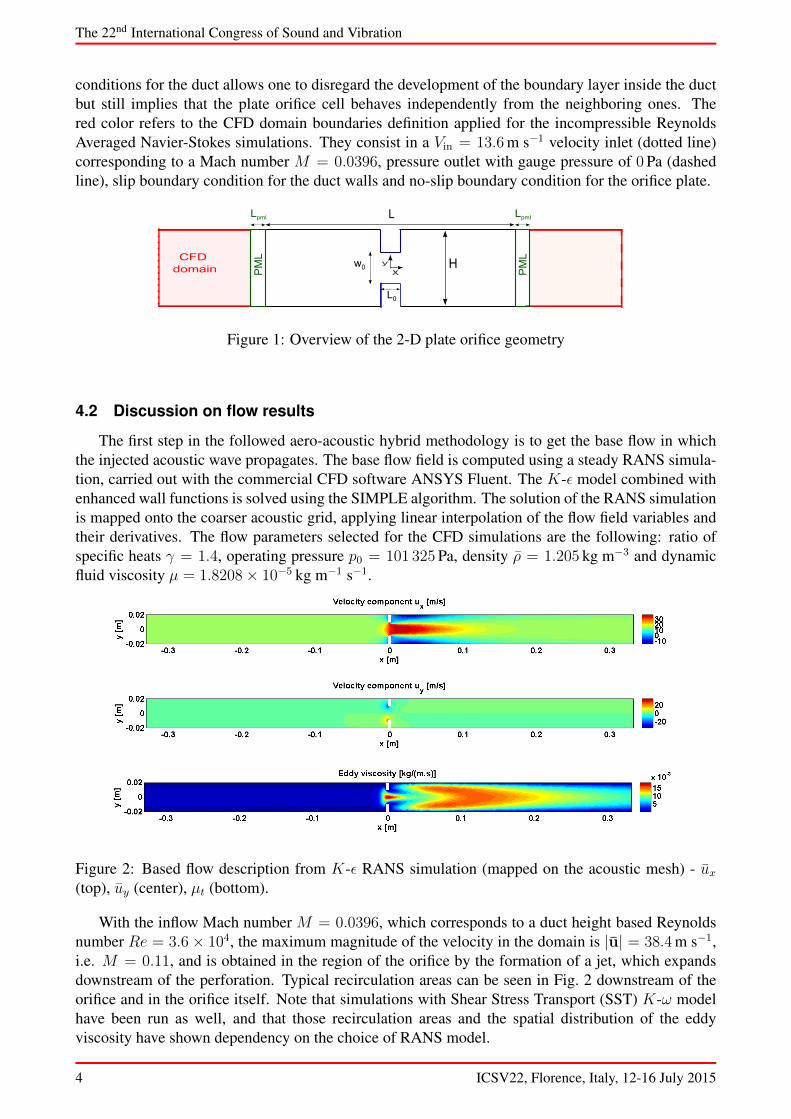
This work focuses on the acoustic scattering of a plane wave impinging on an orifice plate witha single hole with flow passing through. The computational domain for both Computational FluidDynamics (CFD) and acoustics is depicted in Fig. 1. The physical dimensions of the setup are L0 =0.004 m × w0 = 0.02 m for the perforation and L = 33.2w0 × H = 2w0 for the duct. The PMLdomains for injection of the acoustic modes into the physical domain and non-reflective boundaryconditions have a length LPML = 0.5w0. Boundary conditions for the CFD and LNS models areindicated as well in Fig. 1. Black lines indicate slip wall boundary condition and blue lines refer tono-slip boundary conditions, for both flow and acoustic simulations. Prescribing slip wall boundary

ICSV22, Florence, Italy, 12-16 July 2015 3

The 22nd International Congress of Sound and Vibration

conditions for the duct allows one to disregard the development of the boundary layer inside the ductbut still implies that the plate orifice cell behaves independently from the neighboring ones. Thered color refers to the CFD domain boundaries definition applied for the incompressible ReynoldsAveraged Navier-Stokes simulations. They consist in a Vin = 13.6 m s−1 velocity inlet (dotted line)corresponding to a Mach number M = 0.0396, pressure outlet with gauge pressure of 0 Pa (dashedline), slip boundary condition for the duct walls and no-slip boundary condition for the orifice plate.

HP

ML

PM

LCFD domain

L0

w0

L

xy

Lpml Lpml

Figure 1: Overview of the 2-D plate orifice geometry

4.2 Discussion on flow results

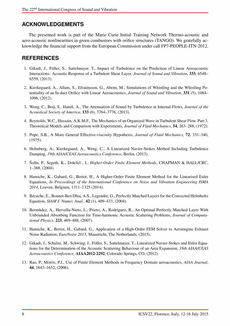
The first step in the followed aero-acoustic hybrid methodology is to get the base flow in whichthe injected acoustic wave propagates. The base flow field is computed using a steady RANS simula-tion, carried out with the commercial CFD software ANSYS Fluent. The K-ε model combined withenhanced wall functions is solved using the SIMPLE algorithm. The solution of the RANS simulationis mapped onto the coarser acoustic grid, applying linear interpolation of the flow field variables andtheir derivatives. The flow parameters selected for the CFD simulations are the following: ratio ofspecific heats γ = 1.4, operating pressure p0 = 101 325 Pa, density ρ = 1.205 kg m−3 and dynamicfluid viscosity µ = 1.8208× 10−5 kg m−1 s−1.

Figure 2: Based flow description from K-ε RANS simulation (mapped on the acoustic mesh) - ux(top), uy (center), µt (bottom).

With the inflow Mach number M = 0.0396, which corresponds to a duct height based Reynoldsnumber Re = 3.6× 104, the maximum magnitude of the velocity in the domain is |u| = 38.4 m s−1,i.e. M = 0.11, and is obtained in the region of the orifice by the formation of a jet, which expandsdownstream of the perforation. Typical recirculation areas can be seen in Fig. 2 downstream of theorifice and in the orifice itself. Note that simulations with Shear Stress Transport (SST) K-ω modelhave been run as well, and that those recirculation areas and the spatial distribution of the eddyviscosity have shown dependency on the choice of RANS model.

4 ICSV22, Florence, Italy, 12-16 July 2015

The 22nd International Congress of Sound and Vibration

4.3 Sound-turbulence interaction at orifice with bias flow

The p-FEM simulations of the coherent fields have been performed on a 2-D computational meshwith approximately 37 000 triangular linear elements and 3th-order interpolating Lobatto polynomialfunctions, yielding a system of about 487000 degrees of freedom. The size of the smallest elementis determined from the Acoustic Boundary Layer (ABL) thickness δa defined in a medium at restas δa =

√2ν/ω. The value taken corresponds to δa,min = δa(f = 5000 Hz) = 3.1015× 10−5 m,

higher limit of the chosen frequency range [200 - 5000] Hz. The frequency step is 200 Hz. The meshelements h inside the orifice are of the size δa,min, whereas the element size is growing outside theduct linearly up to h = 0.005 m at x = ±0.02 m and further away is constant.

Figure 3: Quasi-laminar LNS results for the real part of the density ρ (left, in kg m−3) and velocitycomponent ρux (right, in kg m−2 s−1) perturbations at St = 0.104 (top), St = 0.313 (center), St =0.521 (bottom).

The coherent fields of the density ρ and velocity component ux are shown in Fig. 3 at threedifferent frequencies. The selected dimensionless frequencies St = 0.104, St = 0.3125 and St =0.521 cover the range of frequencies in this study. Strouhal number values are based on the orificethickness Lo and the orifice flow speed by St = f Lo/ |uorifice|. The perturbed field consists of bothacoustic and vortical contributions. The propagating acoustic plane wave can clearly be identifiedwith its related acoustic wavelength λa = (1 + M) c/f , where f is the frequency and c the speedof sound. The hydrodynamic modes originating from the sound-flow interaction near the orificeedges are characterized by their shorter hydrodynamic wavelength λh = |u| /f . The structures of thehydrodynamic modes observed in this study strongly depend on the Strouhal number St. Those modespropagates rather far from the orifice section at lower frequency, and are still significant in magnitudeafter several duct diameters distance. They can therefore pollute acoustic two-port measurementsperformed with microphones in this region. At low Strouhal numbers, the maximum of vorticesmagnitude is higher than at higher St. Over a low frequency range (estimated [600 - 1200] Hz )additional hydrodynamic modes can also propagate through the large recirculation areas downstreamof the orifice. Results obtained with quasi-laminar LNS equations depicted in Fig. 3 show similarphenomena as found in a previous study [2], even if they cannot be quantitatively compared becauseof the differences in the flow and the dimensions.

Figure 4 shows the density perturbation ρ obtained from quasi-laminar (top) and turbulent (bot-tom) LNS simulations with two different turbulence RANS models. The choice of the RANS modelaffects the predicted harmonic perturbations through the base flow properties (see quasi-laminar re-sults) but also through the eddy viscosity. In both turbulent cases, the extra damping from the eddyviscosity decreases the amplitude of the vortical structures appearing at the orifice edges. The K-ε

ICSV22, Florence, Italy, 12-16 July 2015 5

The 22nd International Congress of Sound and Vibration

model gives higher values of eddy viscosity inside the orifice than the SST K-ω model, which leadsto an increased impact of the turbulence on the vortices. The effect on the acoustic field itself has tobe further quantified.

Figure 4: Effect of RANS base flow choice on LNS results for the real part of the density perturbationρ (kg m−3) at St = 0.104 (i.e. f = 1000 Hz).

Figure 5: Vorticity field Re(ω) (s−1) at St = 0.104 (i.e. f = 1000 Hz) for the 4 physical models.

Figure 5 shows the real part of the vorticity perturbations, defined as ω = ∂uy/∂x − ∂ux/∂y,in the direct vicinity of the orifice down part for four different physical models at frequency St =0.104: LEE, quasi-laminar LNSE with slip boundary condition (without resolving the ABL), quasi-laminar LNSE with no-slip boundary condition and resolving the ABL, and turbulent LNS with no-slip boundary resolving the ABL (with K-ε model). The same acoustic mesh is used in all cases,with mesh size δa,min inside the duct. This represents around three elements inside the ABL at thefrequency St = 0.104.

6 ICSV22, Florence, Italy, 12-16 July 2015

The 22nd International Congress of Sound and Vibration

Vorticity is shed at the leading edge and is convected along the base flow streamlines. The choiceof the physical model plays an important role on the local representation of the interactions betweenacoustic and hydrodynamic modes in the orifice region. The addition of no-slip condition prevents theappearance of spurious modes inside the ABL and an acoustic boundary layer is formed at the orificeplate wall. The addition of fluid and eddy viscosity reduces the amplitude of the vorticity but the edgeshave still the dominant impact on the vorticity. The representation scale in Fig. 5 has been adaptedfor each case, as amplitudes of the vorticity real part change up to two orders the more diffusion isadded to the model, with LEE showing the highest values. Note that the computation of the vorticityfield is performed element by element and therefore one can notice discontinuities between elementswhen their size is large enough. From the simulations results, it can be observed that not only arefinement of the acoustic mesh is needed in the orifice region but also in the area of strong baseflow gradients caused by the orifice shear. If asymmetries in the harmonic field appear at the orificeedges, such refinement however tends to amplify the asymmetric behavior of the downstream results.This behavior was not observed in reference [2] with reported mesh, where mesh size growth ratewas significant also in the downstream area. The local refinement of the mesh inside the orificeimproves the accuracy of the computed perturbations since it captures better the complex sound-flowinteractions localized in the acoustic and turbulent boundary layers. If this area is not refined enough,the error generated inside the orifice can propagate downstream in the shear region.

5. Discussion and conclusion

This paper has presented the results of the simulation of the acoustic propagation through a plateorifice in presence of a bias flow, at low Mach Number (M=0.0396). For this purpose, a hybrid ap-proach was applied, combining RANS steady base flow simulations and linearized acoustic operatorsused to compute the harmonic perturbations. Different physical models for the flow-sound interactionhave been implemented in a frequency domain high-order continuous Finite Element Method solverand those models were compared on the orifice plate configuration. This study compares resultscoming from the isentropic version of the Linearized Euler, standard Linearized Navier-Stokes andturbulent Linearized Navier-Stokes equations.

The presented results constitute the first step in the study of sound-turbulence interaction for anorifice with bias flow. A detailed description of the coherent perturbations due to the acoustic excita-tion of the orifice has been given. In the quasi-laminar assumption, the vortex growth is limited solelyby the fluid viscosity. In case of turbulent LNS equations, the vortical structures due to interactionof acoustic and vorticity modes are damped by the extra terms coming from the added eddy viscos-ity. From the present study, one can see that the extra diffusive terms linked to the effect of the flowturbulence on the coherent perturbation predominantly affect the vortices propagating downstream inthe vicinity of the orifice. Nevertheless, looking at the changes in the global perturbation fields dueto the added viscosity, an impact on the global acoustic behavior can be expected. This has to befurther assessed, e.g. by scattering matrix representation. It has been noticed that the choice of RANSmodels for the base flow simulation impacts considerably the spatial distribution of eddy viscosityand affects significantly the local coherent modes. The turbulence model used for the descriptionof the perturbation Reynolds stress τij in this study is the Newtonian eddy model. Such model hasalready shown some limitations at sufficiently low frequencies in previous studies on duct acousticwith turbulent low Mach number flows. Alternatives, like the frequency dependent eddy-viscositymodels and non-equilibrium models of the turbulent diffusion, could be implemented in the frameof the present p-FEM LNS equations solver to study their impact on the results. Future work willinvestigate the impact of these turbulence effects on the acoustic impedance and a possible extensionof existing impedance models for orifices.

ICSV22, Florence, Italy, 12-16 July 2015 7

The 22nd International Congress of Sound and Vibration

ACKNOWLEDGEMENTS

The presented work is part of the Marie Curie Initial Training Network Thermo-acoustic andaero-acoustic nonlinearities in green combustors with orifice structures (TANGO). We gratefully ac-knowledge the financial support from the European Commission under call FP7-PEOPLE-ITN-2012.

REFERENCES

1. Gikadi, J., Föller, S., Sattelmayer, T., Impact of Turbulence on the Prediction of Linear AeroacousticInteractions: Acoustic Response of a Turbulent Shear Layer, Journal of Sound and Vibration, 333, 6548–6559, (2013).

2. Kierkegaard, A., Allam, S., Efraimsson, G., Abom, M., Simulations of Whistling and the Whistling Po-tentiality of an In-duct Orifice with Linear Aeroacoustics, Journal of Sound and Vibration, 331 (5), 1084–1096, (2012).

3. Weng, C., Boij, S., Hanifi, A., The Attenuation of Sound by Turbulence in Internal Flows, Journal of theAcoustical Society of America, 133 (6), 3764–3776, (2013).

4. Reynolds, W.C., Hussain, A.K.M.F., The Mechanics of an Organized Wave in Turbulent Shear Flow. Part 3.Theoretical Models and Comparison with Experiments, Journal of Fluid Mechanics, 54, 263–288, (1972).

5. Pope, S.B., A More General Effective-viscosity Hypothesis, Journal of Fluid Mechanics, 72, 331–340,(1975).

6. Holmberg, A., Kierkegaard, A., Weng, C., A Linearized Navier-Stokes Method Including TurbulenceDamping, 19th AIAA/CEAS Aeroacoustics Conference, Berlin, (2013).

7. Šolín, P., Segeth, K., Doležel , I., Higher-Order Finite Element Methods, CHAPMAN & HALL/CRC,1–388, (2004).

8. Hamiche, K., Gabard, G., Beriot, H., A Higher-Order Finite Element Method for the Linearised EulerEquations, In Proceedings of the International Conference on Noise and Vibration Engineering ISMA2014, Leuven, Belgium, 1311–1325 (2014).

9. Bécache, E., Bonnet-Ben Dhia, A.S., Legendre, G., Perfectly Matched Layers for the Convected HelmholtzEquation, SIAM J. Numer. Anal., 42 (1), 409–433, (2004).

10. Bermùdez, A., Hervella-Nieto, L., Prieto, A., Rodríguez, R., An Optimal Perfectly Matched Layer WithUnbounded Absorbing Function for Time-harmonic Acoustic Scattering Problems, Journal of Computa-tional Physics, 223, 469–488, (2007).

11. Hamiche, K., Beriot, H., Gabard, G., Application of a High-Order FEM Solver to Aeroengine ExhaustNoise Radiation, EuroNoise 2015, Maastricht, The Netherlands, (2015).

12. Gikadi, J., Schulze, M., Schwing, J., Föller, S., Sattelmayer, T., Linearized Navier-Stokes and Euler Equa-tions for the Determination of the Acoustic Scattering Behaviour of an Area Expansion, 18th AIAA/CEASAeroacoustics Conference, AIAA2012-2292, Colorado Springs, CO, (2012).

13. Rao, P., Morris, P.J., Use of Finite Element Methods in Frequency Domain aeroacoustics, AIAA Journal,44, 1643–1652, (2006).

8 ICSV22, Florence, Italy, 12-16 July 2015