“Who is wise? He that learns from everyone.Who is powerful? He that governs his passion.Who is rich? He that is content.Who is that? Nobody.” Benjamin Franklin
6.1 Introduction
The finite element method (FEM) has its origin in the field of structural analy-sis. Although the earlier mathematical treatment of the method was provided byCourant [1] in 1943, the method was not applied to electromagnetic (EM) problemsuntil 1968. Since then the method has been employed in diverse areas such as waveg-uide problems, electric machines, semiconductor devices, microstrips, and absorptionof EM radiation by biological bodies.
Although the finite difference method (FDM) and the method of moments (MOM)are conceptually simpler and easier to program than the finite element method (FEM),FEM is a more powerful and versatile numerical technique for handling problemsinvolving complex geometries and inhomogeneous media. The systematic generalityof the method makes it possible to construct general-purpose computer programs forsolving a wide range of problems. Consequently, programs developed for a particulardiscipline have been applied successfully to solve problems in a different field withlittle or no modification [2].
The finite element analysis of any problem involves basically four steps [3]:
• discretizing the solution region into a finite number of subregions or elements,
• deriving governing equations for a typical element,
• assembling of all elements in the solution region, and
Discretization of the continuum involves dividing up the solution region into sub-domains, called finite elements. Figure 6.1 shows some typical elements for one-,two-, and three-dimensional problems. The problem of discretization will be fullytreated in Sections 6.5 and 6.6. The other three steps will be described in detail in thesubsequent sections.
As an application of FEM to electrostatic problems, let us apply the four steps men-tioned above to solve Laplace’s equation, ∇2V = 0. For the purpose of illustration,we will strictly follow the four steps mentioned above.
6.2.1 Finite Element Discretization
To find the potential distribution V (x, y) for the two-dimensional solution regionshown in Fig. 6.2(a), we divide the region into a number of finite elements as il-lustrated in Fig. 6.2(b). In Fig. 6.2(b), the solution region is subdivided into nine
nonoverlapping finite elements; elements 6, 8, and 9 are four-node quadrilaterals,while other elements are three-node triangles. In practical situations, however, it ispreferred, for ease of computation, to have elements of the same type throughout theregion. That is, in Fig. 6.2(b), we could have split each quadrilateral into two trianglesso that we have 12 triangular elements altogether. The subdivision of the solutionregion into elements is usually done by hand, but in situations where a large numberof elements is required, automatic schemes to be discussed in Sections 6.5 and 6.6are used.
Figure 6.2(a) The solution region; (b) its finite element discretization.
We seek an approximation for the potential Ve within an element e and then interre-late the potential distribution in various elements such that the potential is continuousacross interelement boundaries. The approximate solution for the whole region is
V (x, y) �N∑e=1
Ve(x, y), (6.1)
whereN is the number of triangular elements into which the solution region is divided.The most common form of approximation for Ve within an element is polynomialapproximation, namely,
for a quadrilateral element. The constants a, b, c, and d are to be determined. Thepotential Ve in general is nonzero within element e but zero outside e. In view ofthe fact that quadrilateral elements do not conform to curved boundary as easily astriangular elements, we prefer to use triangular elements throughout our analysis inthis chapter. Notice that our assumption of linear variation of potential within thetriangular element as in Eq. (6.2) is the same as assuming that the electric field isuniform within the element, i.e.,
Ee = −∇Ve = −(bax + cay
)(6.4)
6.2.2 Element Governing Equations
Consider a typical triangular element shown in Fig. 6.3. The potential Ve1, Ve2,and Ve3 at nodes 1, 2, and 3, respectively, are obtained using Eq. (6.2), i.e.,
Ve1Ve2Ve3
=
1 x1 y1
1 x2 y21 x3 y3
abc
(6.5)
The coefficients a, b and c are determined from Eq. (6.5) asabc
The value of A is positive if the nodes are numbered counterclockwise (starting fromany node) as shown by the arrow in Fig. 6.3. Note that Eq. (6.7) gives the potential
Figure 6.3Typical triangular element; local node numbering 1-2-3 must proceed counter-clockwise as indicated by the arrow.
at any point (x, y) within the element provided that the potentials at the vertices areknown. This is unlike finite difference analysis, where the potential is known at thegrid points only. Also note that αi are linear interpolation functions. They are calledthe element shape functions and they have the following properties [4]:
αi ={
1, i = j
0, i �= j(6.10a)
3∑i=1
αi(x, y) = 1 (6.10b)
The shape functions α1, α2, and α3 are illustrated in Fig. 6.4.The functional corresponding to Laplace’s equation, ∇2V = 0, is given by
Having considered a typical element, the next step is to assemble all such elementsin the solution region. The energy associated with the assemblage of elements is
n is the number of nodes, N is the number of elements, and [C] is called the overall orglobal coefficient matrix, which is the assemblage of individual element coefficientmatrices. Notice that to obtain Eq. (6.19), we have assumed that the whole solutionregion is homogeneous so that ε is constant. For an inhomogeneous solution regionsuch as shown in Fig. 6.5, for example, the region is discretized such that each finiteelement is homogeneous. In this case, Eq. (6.11) still holds, but Eq. (6.19) doesnot apply since ε(= εrεo) or simply εr varies from element to element. To applyEq. (6.19), we may replace ε by εo and multiply the integrand in Eq. (6.14) by εr .
Figure 6.5Discretization of an inhomogeneous solution region.
The process by which individual element coefficient matrices are assembled toobtain the global coefficient matrix is best illustrated with an example. Consider thefinite element mesh consisting of three finite elements as shown in Fig. 6.6. Observe
Figure 6.6Assembly of three elements; i-j -k corresponds to local numbering (1-2-3) of theelement in Fig. 6.3.
the numberings of the mesh. The numbering of nodes 1, 2, 3, 4, and 5 is called globalnumbering. The numbering i-j -k is called local numbering, and it corresponds with1 - 2 - 3 of the element in Fig. 6.3. For example, for element 3 in Fig. 6.6, theglobal numbering 3 - 5 - 4 corresponds with local numbering 1 - 2 - 3 of the elementin Fig. 6.3. (Note that the local numbering must be in counterclockwise sequencestarting from any node of the element.) For element 3, we could choose 4 - 3 - 5
instead of 3 - 5 - 4 to correspond with 1 - 2 - 3 of the element in Fig. 6.3. Thus thenumbering in Fig. 6.6 is not unique. But whichever numbering is used, the globalcoefficient matrix remains the same. Assuming the particular numbering in Fig. 6.6,the global coefficient matrix is expected to have the form
which is a 5 × 5 matrix since five nodes (n = 5) are involved. Again, Cij is thecoupling between nodes i and j . We obtain Cij by using the fact that the potentialdistribution must be continuous across interelement boundaries. The contributionto the i, j position in [C] comes from all elements containing nodes i and j . Forexample, in Fig. 6.6, elements 1 and 2 have node 1 in common; hence
C11 = C(1)11 + C
(2)11 (6.22a)
Node 2 belongs to element 1 only; hence
C22 = C(1)33 (6.22b)
Node 4 belongs to elements 1, 2, and 3; consequently
C44 = C(1)22 + C
(2)33 + C
(3)33 (6.22c)
Nodes 1 and 4 belong simultaneously to elements 1 and 2; hence
C14 = C41 = C(1)12 + C
(2)13 (6.22d)
Since there is no coupling (or direct link) between nodes 2 and 3,
C23 = C32 = 0 (6.22e)
Continuing in this manner, we obtain all the terms in the global coefficient matrix byinspection of Fig. 6.6 as
Note that element coefficient matrices overlap at nodes shared by elements and thatthere are 27 terms (9 for each of the 3 elements) in the global coefficient matrix [C].Also note the following properties of the matrix [C]:
(1) It is symmetric (Cij = Cji) just as the element coefficient matrix.
(2) Since Cij = 0 if no coupling exists between nodes i and j , it is expected thatfor a large number of elements [C] becomes sparse. Matrix [C] is also bandedif the nodes are carefully numbered. It can be shown using Eq. (6.17) that
3∑i=1
C(e)ij = 0 =
3∑j=1
C(e)ij
(3) It is singular. Although this is not so obvious, it can be shown using the elementcoefficient matrix of Eq. (6.16b).
6.2.4 Solving the Resulting Equations
Using the concepts developed in Chapter 4, it can be shown that Laplace’s equationis satisfied when the total energy in the solution region is minimum. Thus we requirethat the partial derivatives of W with respect to each nodal value of the potential bezero, i.e.,
∂W
∂V1= ∂W
∂V2= · · · = ∂W
∂Vn
= 0
or
∂W
∂Vk
= 0, k = 1, 2, . . . , n (6.24)
For example, to get∂W
∂V1= 0 for the finite element mesh of Fig. 6.6, we substitute
Eq. (6.21) into Eq. (6.19) and take the partial derivative of W with respect to V1. Weobtain
where n is the number of nodes in the mesh. By writing Eq. (6.26) for all nodesk = 1, 2, . . . , n, we obtain a set of simultaneous equations from which the solutionof [V ]t = [V1, V2, . . . , Vn] can be found. This can be done in two ways similar tothose used in solving finite difference equations obtained from Laplace’s equation inSection 3.5.
(1) Iteration Method: Suppose node 1 in Fig. 6.6, for example, is a free node. FromEq. (6.25),
V1 = − 1
C11
5∑i=2
ViC1i (6.27)
Thus, in general, at node k in a mesh with n nodes
Vk = − 1
Ckk
n∑i=1,i �=k
ViCki (6.28)
where node k is a free node. Since Cki = 0 if node k is not directly connected tonode i, only nodes that are directly linked to node k contribute to Vk in Eq. (6.28).Equation (6.28) can be applied iteratively to all the free nodes. The iteration processbegins by setting the potentials of fixed nodes (where the potentials are prescribedor known) to their prescribed values and the potentials at the free nodes (where thepotentials are unknown) equal to zero or to the average potential [5]
Vave = 1
2(Vmin + Vmax) (6.29)
where Vmin and Vmax are the minimum and maximum values of V at the fixed nodes.With these initial values, the potentials at the free nodes are calculated using Eq. (6.28).At the end of the first iteration, when the new values have been calculated for all thefree nodes, they become the old values for the second iteration. The procedure isrepeated until the change between subsequent iterations is negligible enough.
(2) Band Matrix Method: If all free nodes are numbered first and the fixed nodeslast, Eq. (6.19) can be written such that [4]
W = 1
2ε[Vf Vp
] [Cff Cfp
Cpf Cpp
] [Vf
Vp
](6.30)
where subscripts f and p, respectively, refer to nodes with free and fixed (or pre-scribed) potentials. Since Vp is constant (it consists of known, fixed values), we onlydifferentiate with respect to Vf so that applying Eqs. (6.24) to (6.30) yields
where [V ] = [Vf ], [A] = [Cff ], [B] = −[Cfp][Vp]. Since [A] is, in general,nonsingular, the potential at the free nodes can be found using Eq. (6.32). We cansolve for [V ] in Eq. (6.32a) using Gaussian elimination technique. We can also solvefor [V ] in Eq. (6.32b) using matrix inversion if the size of the matrix to be inverted isnot large.
It is sometimes necessary to impose Neumann condition (∂V
∂n= 0) as a boundary
condition or at the line of symmetry when we take advantage of the symmetry of theproblem. Suppose, for concreteness, that a solution region is symmetric along the
y-axis as in Fig. 6.7. We impose condition (∂V
∂x= 0) along the y-axis by making
V1 = V2, V4 = V5, V7 = V8 (6.33)
Figure 6.7A solution region that is symmetric along the y-axis.
Notice that as from Eq. (6.11) onward, the solution has been restricted to a two-dimensional problem involving Laplace’s equation, ∇2V = 0. The basic conceptsdeveloped in this section will be extended to finite element analysis of problemsinvolving Poisson’s equation (∇2V = −ρv/ε, ∇2A = −µJ) or wave equation(∇2#− γ 2# = 0) in the next sections.
Cij . This may be used to check ifC is properly obtained.
We now apply Eq. (6.28) to the free nodes 2 and 4, i.e.,
V2 = − 1
C22(V1C12 + V3C32 + V4C42)
V4 = − 1
C44(V1C14 + V2C24 + V3C34)
or
V2 = − 1
1.25(−4.571− 0.0143V4) (6.39a)
V4 = − 1
0.8381(−0.143V2 − 3.667) (6.39b)
By initially setting V2 = 0 = V4, we apply Eqs. (6.39a), (6.39b) iteratively. Thefirst iteration gives V2 = 3.6568, V4 = 4.4378 and at the second iteration V2 =3.7075, V4 = 4.4386. Just after two iterations, we obtain the same results as thosefrom the band matrix method [3]. Thus the iterative technique is faster and is usuallypreferred for a large number of nodes. Once the values of the potentials at the nodes areknown, the potential at any point within the mesh can be determined using Eq. (6.7).
Example 6.2Write a FORTRAN program to solve Laplace’s equation using the finite element
method. Apply the program to the two-dimensional problem shown in Fig. 6.9(a).
Figure 6.9For Example 6.2: (a) Two-dimensional electrostatic problem, (b) solution regiondivided into 25 triangular elements.
Solution
The solution region is divided into 25 three-node triangular elements with total numberof nodes being 21 as shown in Fig. 6.9(b). This is a necessary step in order to have inputdata defining the geometry of the problem. Based on the discussions in Section 6.2, ageneral FORTRAN program for solving problems involving Laplace’s equation usingthree-node triangular elements is developed as shown in Fig. 6.10. The developmentof the program basically involves four steps indicated in the program and explainedas follows.
Step 1: This involves inputting the necessary data defining the problem. This is theonly step that depends on the geometry of the problem at hand. Through a data file,we input the number of elements, the number of nodes, the number of fixed nodes,the prescribed values of the potentials at the free nodes, the x and y coordinates ofall nodes, and a list identifying the nodes belonging to each element in the order ofthe local numbering 1 - 2 - 3. For the problem in Fig. 6.9, the three sets of data forcoordinates, element-node relationship, and prescribed potentials at fixed nodes areshown in Tables 6.1, 6.2, and 6.3, respectively.
Step 2: This step entails finding the element coefficient matrix [C(e)] for each elementand using the terms to form the global matrix [C].Step 3: At this stage, we first find the list of free nodes using the given list ofprescribed nodes. We now apply Eq. (6.28) iteratively to all the free nodes. Thesolution converges at 50 iterations or less since only 6 nodes are involved in this case.The solution obtained is exactly the same as those obtained using the band matrixmethod [3].
Step 4: This involves outputting the result of the computation. The output data forthe problem in Fig. 6.9 is presented in Table 6.4. The validity of the result in Table 6.4is checked using the finite difference method. From the finite difference analysis, the
Although the result obtained using finite difference is considered more accurate in thisproblem, increased accuracy of finite element analysis can be obtained by dividing thesolution region into a greater number of triangular elements, or using higher-orderelements to be discussed in Section 6.8. As alluded to earlier, the finite elementmethod has two major advantages over the finite difference method. Field quantitiesare obtained only at discrete positions in the solution region using FDM; they canbe obtained at any point in the solution region in FEM. Also, it is easier to handlecomplex geometries using FEM than using FDM.
6.3 Solution of Poisson’s Equation
To solve the two-dimensional Poisson’s equation,
∇2V = −ρs
ε(6.40)
using FEM, we take the same steps as in Section 6.2. Since the steps are essentiallythe same as in Section 6.2 except that we must include the source term, only the majordifferences will be highlighted here.
6.3.1 Deriving Element-governing Equations
After the solution region is divided into triangular elements, we approximate thepotential distribution Ve(x, y) and the source term ρse (for two-dimensional prob-lems) over each triangular element by linear combinations of the local interpolationpolynomial αi , i.e.,
Ve =3∑
i=1
Veiαi(x, y) (6.41)
ρse =3∑
i=1
ρeiαi(x, y) (6.42)
The coefficients Vei and ρei , respectively, represent the values of V and ρs at vertex i
of element e as in Fig. 6.3. The values of ρei are known since ρs(x, y) is prescribed,while the values of Vei are to be determined.
From Table 4.1, an energy functional whose associated Euler equation is Eq. (6.40)is
F (Ve) = 1
2
∫S
[ε |∇Ve|2 − 2ρseVe
]dS (6.43)
F(Ve) represents the total energy per length within element e. The first term under the
integral sign,1
2D · E = 1
2ε|∇Ve|2, is the energy density in the electrostatic system,
while the second term, ρseVedS, is the work done in moving the charge ρsedS to itslocation at potential Ve. Substitution of Eqs. (6.41) and (6.42) into Eq. (6.43) yields
F (Ve) = 1
2
3∑i=1
3∑j=1
εVei
[∫∇αi · ∇αj dS
]Vej
−3∑
i=1
3∑j=1
Vei
[∫αiαj dS
]ρej
This can be written in matrix form as
F (Ve) = 1
2ε[Ve
]t [C(e)
][Ve
]− [Ve
]t [T (e)
][ρe]
(6.44)
where
C(e)ij =
∫∇αi · ∇αj dS (6.45)
which is already defined in Eq. (6.17) and
T(e)ij =
∫αiαj dS (6.46)
It will be shown in Section 6.8 that
T(e)ij =
{A/12, i �= j
A/6 i = j(6.47)
where A is the area of the triangular element.Equation (6.44) can be applied to every element in the solution region. We obtain
the discretized functional for the whole solution region (withN elements and n nodes)as the sum of the functionals for the individual elements, i.e., from Eq. (6.44),
F(V ) =N∑e=1
F (Ve) = 1
2ε[V ]t [C][V ] − [V ]t [T ][ρ] (6.48)
where t denotes transposition. In Eq. (6.48), the column matrix [V ] consists of thevalues of Vei , while the column matrix [ρ] contains n values of the source function ρsat the nodes. The functional in Eq. (6.48) is now minimized by differentiating withrespect to Vei and setting the result equal to zero.
where node k is assumed to be a free node.By fixing the potential at the prescribed nodes and setting the potential at the free
nodes initially equal to zero, we apply Eq. (6.52) iteratively to all free nodes untilconvergence is reached.
Band Matrix Method: If we choose to solve the problem using the band matrixmethod, we let the free nodes be numbered first and the prescribed nodes last. By
where [A] = [Cff ], [V ] = [Vf ] and [B] is the right-hand side of Eq. (6.54). Equa-tion (6.55) can be solved to determine [V ] either by matrix inversion or Gaussianelimination technique discussed in Appendix D. There is little point in giving ex-amples on applying FEM to Poisson’s problems, especially when it is noted that thedifference between Eqs. (6.28) and (6.52) or Eqs. (6.54) and (6.31) is slight. See [19]for an example.
6.4 Solution of the Wave Equation
A typical wave equation is the inhomogeneous scalar Helmholtz’s equation
∇2#+ k2# = g (6.56)
where # is the field quantity (for waveguide problem, # = Hz for TE mode or Ez
for TM mode) to be determined, g is the source function, and k = ω√µε is the
wave number of the medium. The following three distinct special cases of Eq. (6.56)should be noted:
(i) k = 0 = g: Laplace’s equation;
(ii) k = 0: Poisson’s equation; and
(iii) k is an unknown, g = 0: homogeneous, scalar Helmholtz’s equation.
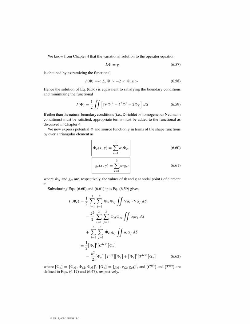
We know from Chapter 4 that the variational solution to the operator equation
L# = g (6.57)
is obtained by extremizing the functional
I (#) =< L,# > −2 < #, g > (6.58)
Hence the solution of Eq. (6.56) is equivalent to satisfying the boundary conditionsand minimizing the functional
I (#) = 1
2
∫∫ [|∇#|2 − k2#2 + 2#g
]dS (6.59)
If other than the natural boundary conditions (i.e., Dirichlet or homogeneous Neumannconditions) must be satisfied, appropriate terms must be added to the functional asdiscussed in Chapter 4.
We now express potential # and source function g in terms of the shape functionsαi over a triangular element as
#e(x, y) =3∑
i=1
αi#ei (6.60)
ge(x, y) =3∑
i=1
αigei (6.61)
where #ei and gei are, respectively, the values of # and g at nodal point i of elemente.
Substituting Eqs. (6.60) and (6.61) into Eq. (6.59) gives
I (#e) = 1
2
3∑i=1
3∑j=1
#ei#ej
∫∫∇αi · ∇αj dS
− k2
2
3∑i=1
3∑j=1
#ei#ej
∫∫αiαj dS
+3∑
i=1
3∑j=1
#eigej
∫∫αiαj dS
= 1
2
[#e
]t [C(e)
][#e
]− k2
2
[#e
]t [T (e)
][#e
]+ [#e
]t [T (e)
][Ge
](6.62)
where [#e] = [#e1,#e2,#e3]t , [Ge] = [ge1, ge2, ge3]t , and [C(e)] and [T (e)] aredefined in Eqs. (6.17) and (6.47), respectively.
Equation (6.62), derived for a single element, can be applied for all N elements inthe solution region. Thus,
I (#) =N∑e=1
I (#e) (6.63)
From Eqs. (6.62) and (6.63), I (#) can be expressed in matrix form as
I (#) = 1
2[#]t [C][#] − k2
2[#]t [T ][#] + [#]t [T ][G] (6.64)
where
[#] = [#1,#2, . . . , #N ]t , (6.65a)
[G] = [g1, g2, . . . , gN ]t , (6.65b)
[C], and [T ] are global matrices consisting of local matrices [C(e)] and [T (e)], re-spectively.
Consider the special case in which the source function g = 0. Again, if free nodesare numbered first and the prescribed nodes last, we may write Eq. (6.64) as
where I is a unit matrix. Any standard procedure [7] (or see Appendix D) maybe used to obtain some or all of the eigenvalues λ1, λ2, . . . , λnf and eigenvectorsX1, X2, . . . , Xnf , where nf is the number of free nodes. The eigenvalues are alwaysreal since C and T are symmetric.
Solution of the algebraic eigenvalue problems in Eq. (6.70) furnishes eigenvaluesand eigenvectors, which form good approximations to the eigenvalues and eigenfunc-tions of the Helmholtz problem, i.e., the cuttoff wavelengths and field distributionpatterns of the various modes possible in a given waveguide.
The solution of the problem presented in this section, as summarized in Eq. (6.69),can be viewed as the finite element solution of homogeneous waveguides. The ideacan be extended to handle inhomogeneous waveguide problems [8]–[11]. However,in applying FEM to inhomogeneous problems, a serious difficulty is the appearance ofspurious, nonphysical solutions. Several techniques have been proposed to overcomethe difficulty [12]–[18].
Example 6.3To apply the ideas presented in this section, we use the finite element analysis to
determine the lowest (or dominant) cutoff wavenumber kc of the TM11 mode inwaveguides with square (a× a) and rectangular (a× b) cross sections for which theexact results are already known as
kc =√(mπ/a)2 + (nπ/b)2
where m = n = 1.It may be instructive to try with hand calculation the case of a square waveguide
with 2 divisions in the x and y directions. In this case, there are 9 nodes, 8 triangularelements, and 1 free node (nf = 1). Equation (6.68) becomes
C11 − k2T11 = 0
where C11 and T11 are obtained from Eqs. (6.34), (6.35), and (6.47) as
which is about 27% off the exact solution. To improve the accuracy, we must usemore elements.
The computer program in Fig. 6.11 applies the ideas in this section to find kc. Themain program calls subroutine GRID (to be discussed in Section 6.5) to generate thenecessary input data from a given geometry. Ifnx andny are the number of divisions inthex andy directions, the total number of elementsne = 2nxny . By simply specifyingthe values of a, b, nx , and ny , the program determines kc using subroutines GRID,INVERSE, and POWER or EIGEN. Subroutine INVERSE available in Appendix Dfinds T −1
ff required in Eq. (6.70a). Either subroutine POWER or EIGEN calculatesthe eigenvalues. EIGEN finds all the eigenvalues, while POWER only determines thelowest eigenvalue; both subroutines are available in Appendix D. The results for thesquare (a = b) and rectangular (b = 2a) waveguides are presented in Tables 6.5aand 6.5b, respectively.
Table 6.5 (a) LowestWavenumber for a SquareWaveguide (b = a)
Figure 6.11(Cont.) Computer program for Example 6.3.
6.5 Automatic Mesh Generation I — Rectangular Domains
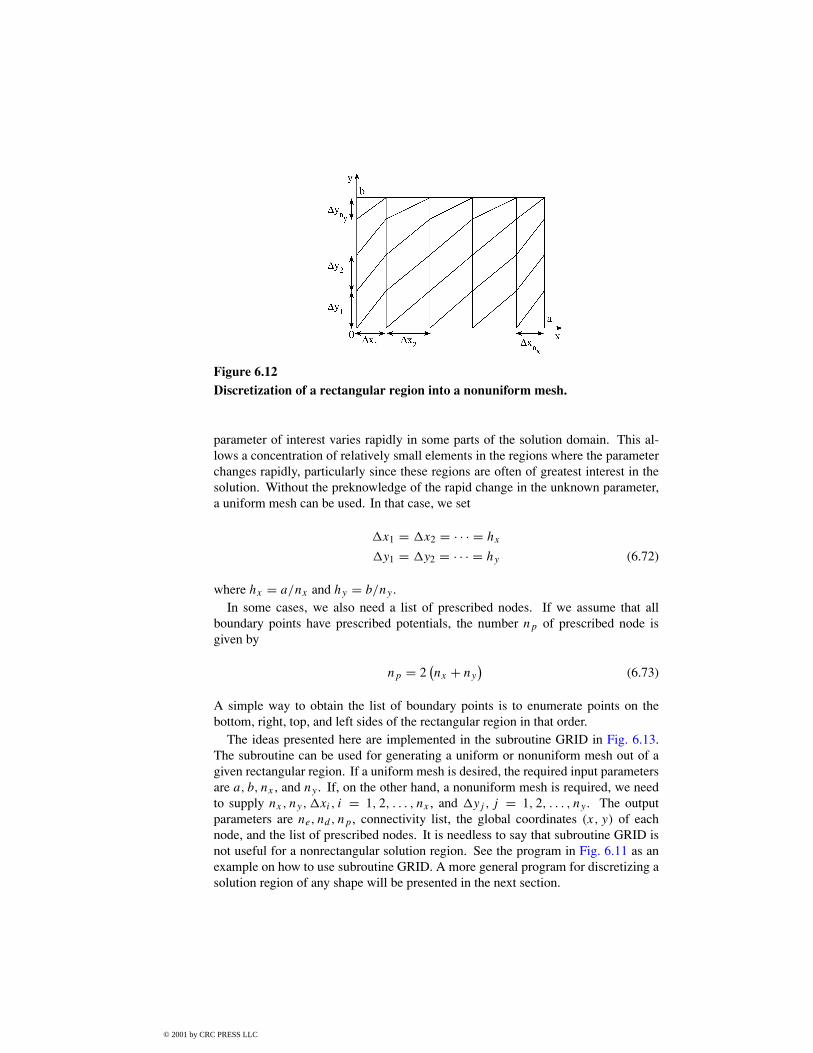
One of the major difficulties encountered in the finite element analysis of con-tinuum problems is the tedious and time-consuming effort required in data preparation.Efficient finite element programs must have node and element generating schemes,referred to collectively as mesh generators. Automatic mesh generation minimizesthe input data required to specify a problem. It not only reduces the time involvedin data preparation, it eliminates human errors introduced when data preparationis performed manually. Combining the automatic mesh generation program withcomputer graphics is particularly valuable since the output can be monitored visually.Since some applications of the FEM to EM problems involve simple rectangulardomains, we consider the generation of simple meshes [19] here; automatic meshgenerator for arbitrary domains will be discussed in Section 6.6.
Consider a rectangular solution region of size a × b as in Fig. 6.12. Our goal isto divide the region into rectangular elements, each of which is later divided intotwo triangular elements. Suppose nx and ny are the number of divisions in x and y
directions, the total number of elements and nodes are, respectively, given by
ne = 2 nxny
nd = (nx + 1)(ny + 1
) (6.71)
Thus it is easy to figure out from Fig. 6.12 a systematic way of numbering the elementsand nodes. To obtain the global coordinates (x, y) for each node, we need an arraycontaining 9xi, i = 1, 2, . . . , nx and 9yj , j = 1, 2, . . . , ny , which are, respectively,the distances between nodes in the x and y directions. If the order of node numberingis from left to right along horizontal rows and from bottom to top along the verticalrows, then the first node is the origin (0,0). The next node is obtained as x → x+9x1while y = 0 remains unchanged. The following node has x → x +9x2, y = 0, andso on until 9xi are exhausted. We start the second next horizontal row by startingwith x = 0, y → y +9y1 and increasing x until 9xi are exhausted. We repeat theprocess until the last node (nx + 1)(ny + 1) is reached, i.e., when 9xi and 9yi areexhausted simultaneously.
The procedure presented here allows for generating uniform and nonuniformmeshes. A mesh is uniform if all 9xi are equal and all 9yi are equal; it is nonuni-form otherwise. A nonuniform mesh is preferred if it is known in advance that the
Figure 6.12Discretization of a rectangular region into a nonuniform mesh.
parameter of interest varies rapidly in some parts of the solution domain. This al-lows a concentration of relatively small elements in the regions where the parameterchanges rapidly, particularly since these regions are often of greatest interest in thesolution. Without the preknowledge of the rapid change in the unknown parameter,a uniform mesh can be used. In that case, we set
9x1 = 9x2 = · · · = hx
9y1 = 9y2 = · · · = hy (6.72)
where hx = a/nx and hy = b/ny .In some cases, we also need a list of prescribed nodes. If we assume that all
boundary points have prescribed potentials, the number np of prescribed node isgiven by
np = 2(nx + ny
)(6.73)
A simple way to obtain the list of boundary points is to enumerate points on thebottom, right, top, and left sides of the rectangular region in that order.
The ideas presented here are implemented in the subroutine GRID in Fig. 6.13.The subroutine can be used for generating a uniform or nonuniform mesh out of agiven rectangular region. If a uniform mesh is desired, the required input parametersare a, b, nx , and ny . If, on the other hand, a nonuniform mesh is required, we needto supply nx, ny,9xi, i = 1, 2, . . . , nx , and 9yj , j = 1, 2, . . . , ny . The outputparameters are ne, nd, np, connectivity list, the global coordinates (x, y) of eachnode, and the list of prescribed nodes. It is needless to say that subroutine GRID isnot useful for a nonrectangular solution region. See the program in Fig. 6.11 as anexample on how to use subroutine GRID. A more general program for discretizing asolution region of any shape will be presented in the next section.
6.6 Automatic Mesh Generation II — Arbitrary Domains
As the solution regions become more complex than the ones considered in Sec-tion 6.5, the task of developing mesh generators becomes more tedious. A number ofmesh generation algorithms (e.g., [21]–[33]) of varying degrees of automation havebeen proposed for arbitrary solution domains. Reviews of various mesh generationtechniques can be found in [34, 35].
The basic steps involved in a mesh generation are as follows [36]:
• subdivide solution region into few quadrilateral blocks,
The solution region is subdivided into quadrilateral blocks. Subdomains with dif-ferent constitutive parameters (σ, µ, ε) must be represented by separate blocks. Asinput data, we specify block topologies and the coordinates at eight points describingeach block. Each block is represented by an eight-node quadratic isoparametric ele-ment. With natural coordinate system (ζ, η), the x and y coordinates are representedas
x(ζ, η) =8∑
i=1
αi(ζ, η) xi (6.74)
y(ζ, η) =8∑
i=1
αi(ζ, η) yi (6.75)
where αi(ζ, η) is a shape function associated with node i, and (xi, yi) are the coordi-nates of node i defining the boundary of the quadrilateral block as shown in Fig. 6.14.The shape functions are expressed in terms of the quadratic or parabolic isoparametricelements shown in Fig. 6.15. They are given by:
For each block, we specify N DIVX and N DIVY , the number of element sub-divisions to be made in the ζ and η directions, respectively. Also, we specify theweighting factors (Wζ )i and (Wη)i allowing for graded mesh within a block. Inspecifying N DIVX,N DIVY,Wζ , and Wη care must be taken to ensure that the sub-division along block interfaces (for adjacent blocks) are compatible. We initialize ζ
and η to a value of −1 so that the natural coordinates are incremented according to
Three element types are permitted: (a) linear four-node quadrilateral elements,(b) linear three-node triangular elements, (c) quadratic eight-node isoparametric ele-ments.
6.6.3 Connection of Individual Blocks
After subdividing each block and numbering its nodal points separately, it is nec-essary to connect the blocks and have each node numbered uniquely. This is ac-complished by comparing the coordinates of all nodal points and assigning the samenumber to all nodes having identical coordinates. That is, we compare the coordi-nates of node 1 with all other nodes, and then node 2 with other nodes, etc., untilall repeated nodes are eliminated. The listing of the FORTRAN code for automaticmesh generation is shown in Fig. 6.16; it is essentially a modified version of the onein Hinton and Owen [36]. The following example taken from [36] illustrates theapplication of the code.
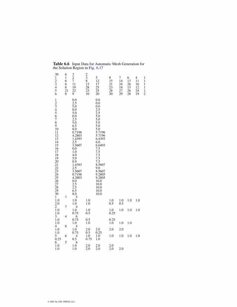
Example 6.4Use the code in Fig. 6.16 to discretize the mesh in Fig. 6.17.
SolutionThe input data for the mesh generation is presented in Table 6.6. The subroutineINPUT reads the number of points (NPOIN) defining the mesh, the number ofblocks (NELEM), the element type (NNODE), the number of coordinate dimen-sions (NDIME), the nodes defining each block, and the coordinates of each node inthe mesh. The subroutine GENERATE reads the number of divisions and weightingfactors along ζ and η directions for each block. It then subdivides the block intoquadrilateral elements. At this point, the whole input data shown in Table 6.6 havebeen read. The subroutine TRIANGLE divides each four-node quadrilateral elementacross the shorter diagonal. The subroutine OUTPUT provides the coordinates ofthe nodes, element topologies, and material property numbers of the generated mesh.For the input data in Table 6.6, the generated mesh with 200 nodes and 330 elementsis shown in Fig. 6.18.
Figure 6.18The generated mesh corresponding to input data in Table 6.6.
6.7 Bandwidth Reduction
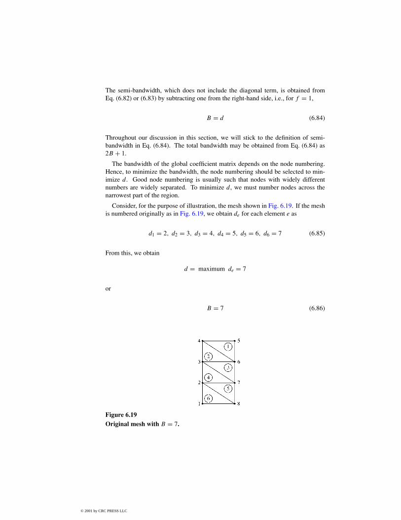
Since most of the matrices involved in FEM are symmetric, sparse, and banded,we can minimize the storage requirements and the solution time by storing only theelements involved in half bandwidth instead of storing the whole matrix. To take thefullest advantage of the benefits from using a banded matrix solution technique, wemust make sure that the matrix bandwidth is as narrow as possible.
If we let d be the maximum difference between the lowest and the highest nodenumbers of any single element in the mesh, we define the semi-bandwidth B (whichincludes the diagonal term) of the coefficient matrix [C] as
B = (d + 1)f (6.82)
where f is the number of degrees of freedom (or number of parameters) at each node.If, for example, we are interested in calculating the electric field intensity E for athree-dimensional problem, then we need Ex,Ey , and Ez at each node, and f = 3in this case. Assuming that there is only one parameter per node,
The semi-bandwidth, which does not include the diagonal term, is obtained fromEq. (6.82) or (6.83) by subtracting one from the right-hand side, i.e., for f = 1,
B = d (6.84)
Throughout our discussion in this section, we will stick to the definition of semi-bandwidth in Eq. (6.84). The total bandwidth may be obtained from Eq. (6.84) as2B + 1.
The bandwidth of the global coefficient matrix depends on the node numbering.Hence, to minimize the bandwidth, the node numbering should be selected to min-imize d . Good node numbering is usually such that nodes with widely differentnumbers are widely separated. To minimize d, we must number nodes across thenarrowest part of the region.
Consider, for the purpose of illustration, the mesh shown in Fig. 6.19. If the meshis numbered originally as in Fig. 6.19, we obtain de for each element e as
Alternatively, the semi-bandwidth may be determined from the coefficient matrix,which is obtained by mere inspection of Fig. 6.19 as
B=7←−−−−−−−−−−−−−−→1 2 3 4 5 6 7 8
[C] =
12345678
x x x
x x x x x
x x x x
x x x x
x x x
x x x x x
x x x x
x x x
(6.87)
where x indicates a possible nonzero term and blanks are zeros (i.e., Cij = 0, indicat-ing no coupling between nodes i and j ). If the mesh is renumbered as in Fig. 6.20(a),
d1 = 4 = d2 = d3 = d4 = d5 = d6 (6.88)
and henced = maximum de = 4
or
B = 4 (6.89)
Figure 6.20Renumbered nodes: (a) B = 4, (b) B = 2.
Finally, we may renumber the mesh as in Fig. 6.20(b). In this case
The value B = 2 may also be obtained from the coefficient matrix for the mesh inFig. 6.20(b), namely,
B=2←−−−→P Q
[C] =
1 2 3 4 5 6 7 812345678
x x x
x x x x
x x x x x
x x x x
x x x x x
x x x x x
x x x x
x x x
R
S
(6.93)
From Eq. (6.93), one immediately notices that [C] is symmetric and that terms areclustered in a band about the diagonal. Hence [C] is sparse and banded so that onlythe data within the area PQRS of the matrix need to be stored—a total of 21 termsout of 64. This illustrates the savings in storage by a careful nodal numbering.
For a simple mesh, hand-labeling coupled with a careful inspection of the mesh (aswe have done so far) can lead to a minimum bandwidth. However, for a large mesh,a hand-labeling technique becomes a tedious, time-consuming task, which in mostcases may not be successful. It is particularly desirable that an automatic relabelingscheme is implemented within a mesh generation program. A number of algorithmshave been proposed for bandwidth reduction by automatic mesh renumbering [37]–[40]. A simple, efficient algorithm is found in Collins [37].
6.8 Higher Order Elements
The finite elements we have used so far have been the linear type in that the shapefunction is of the order one. A higher order element is one in which the shape functionor interpolation polynomial is of the order two or more.
The accuracy of a finite element solution can be improved by using finer mesh orusing higher order elements or both. A discussion on mesh refinement versus higherorder elements is given by Desai and Abel [2]; a motivation for using higher orderelements is given by Csendes in [41]. In general, fewer higher order elements areneeded to achieve the same degree of accuracy in the final results. The higher orderelements are particularly useful when the gradient of the field variable is expectedto vary rapidly. They have been applied with great success in solving EM-relatedproblems [4], [41]–[46].
Higher order triangular elements can be systematically developed with the aid of theso-called Pascal triangle given in Fig. 6.21. The family of finite elements generatedin this manner with the distribution of nodes illustrated in Fig. 6.22. Note that inhigher order elements, some secondary (side and/or interior) nodes are introduced inaddition to the primary (corner) nodes so as to produce exactly the right number ofnodes required to define the shape function of that order. The Pascal triangle containsterms of the basis functions of various degrees in variables x and y. An arbitraryfunction #i(x, y) can be approximated in an element in terms of a complete nthorder polynomial as
#(x, y) =m∑i=1
αi#i (6.94)
where
m = 1
2(n+ 1)(n+ 2) (6.95)
is the number of terms in complete polynomials (also the number of nodes in thetriangle). For example, for second order (n = 2) or quadratic (six-node) triangularelements,
#e(x, y) = a1 + a2x + a3y + a4xy + a5x2 + a6y
2 (6.96)
This equation has six coefficients, and hence the element must have six nodes. Itis also complete through the second order terms. A systematic derivation of theinterpolation function α for the higher order elements involves the use of the localcoordinates.
Figure 6.21The Pascal Triangle. The first row is: (constant, n = 0), the second: (linear,n = 1), the third: (quadratic, n = 2), the fourth: (cubic, n = 3), the fifth:(quartic, n = 4).
Figure 6.22The Pascal triangle and the associated polynomial basis function for degreen = 1to 4.
6.8.2 Local Coordinates
The triangular local coordinates (ξ1, ξ2, ξ3) are related to Cartesian coordinates(x, y) as
x = ξ1x1 + ξ2x2 + ξ3x3 (6.97)
y = ξ1y1 + ξ2y2 + ξ3y3 (6.98)
The local coordinates are dimensionless with values ranging from 0 to 1. Bydefinition, ξi at any point within the triangle is the ratio of the perpendicular distancefrom the point to the side opposite to vertex i to the length of the altitude drawn fromvertex i. Thus, from Fig. 6.23 the value of ξ1 at P, for example, is given by the ratioof the perpendicular distance d from the side opposite vertex 1 to the altitude h ofthat side, i.e.,
ξ1 = d
h(6.99)
Alternatively, from Fig. 6.23, ξi at P can be defined as
ξi = Ai
A(6.100)
so that
ξ1 + ξ2 + ξ3 = 1 (6.101)
since A1 + A2 + A3 = A. In view of Eq. (6.100), the local coordinates ξi are alsocalled area coordinates. The variation of (ξ1, ξ2, ξ3) inside an element is shown in
Fig. 6.24. Although the coordinates ξ1, ξ2, and ξ3 are used to define a point P, only twoare independent since they must satisfy Eq. (6.101). The inverted form of Eqs. (6.97)and (6.98) is
ξi = 1
2A[ci + bix + aiy] (6.102)
where
ai = xk − xj ,bi = yj − yk ,ci = xjyk − xkyjA = area of the triangle = 1
2(b1a2 − b2a1) , (6.103)
and (i, j, k) is an even permutation of (1,2,3). (Notice that ai and bi are the same asQi and Pi in Eq. (6.34).) The differentiation and integration in local coordinates arecarried out using [47]:
∂f
∂ξ1= a2
∂f
∂x− b2
∂f
∂y(6.104a)
∂f
∂ξ2= −a1
∂f
∂x+ b1
∂f
∂y(6.104b)
∂f
∂x= 1
2A
(b1∂f
∂ξ1+ b2
∂f
∂ξ2
)(6.104c)
∂f
∂y= 1
2A
(a1∂f
∂ξ1+ a2
∂f
∂ξ2
)(6.104d)
∫∫f dS = 2A
∫ 1
0
[∫ 1−ξ2
0f (ξ1, ξ2) dξ1
]dξ2 (6.104e)
∫∫ξ i1ξ
j
2 ξk3 dS =
i! j ! k!(i + j + k + 2)!2A (6.104f)
dS = 2Adξ1 dξ2 (6.104g)
6.8.3 Shape Functions
We may now express the shape function for higher order elements in terms of localcoordinates. Sometimes, it is convenient to label each point in the finite elements inFig. 6.22 with three integers i, j , and k from which its local coordinates (ξ1, ξ2, ξ3)
The relationships between the subscripts q ∈ {1, 2, 3} on ξq, � ∈ {1, 2, . . . , m}on α�, and r ∈ (i, j, k) on pr and Pijk in Eqs. (6.107) to (6.109) are illustrated inFig. 6.25 for n ranging from 1 to 4. Henceforth point Pijk will be written as Pn forconciseness.
Figure 6.25Distribution of nodes over triangles for n = 1 to 4. The triangles are in standardposition (Continued).
Figure 6.25(Cont.) Distribution of nodes over triangles for n = 1 to 4. The triangles are instandard position.
Notice from Eq. (6.108) or Eq. (6.109) that
p0(ξ) = 1
p1(ξ) = nξp2(ξ) = 1
2(nξ − 1)nξ
p3(ξ) = 1
6(nξ − 2)(nξ − 1)nξ
p4(ξ) = 1
24(nξ − 3)(nξ − 2)(nξ − 1)nξ, etc (6.110)
Substituting Eq. (6.110) into Eq. (6.107) gives the shape functions α� for nodes� = 1, 2, . . . , m, as shown in Table 6.7 for n = 1 to 4. Observe that each α� takesthe value of 1 at node � and value of 0 at all other nodes in the triangle. This is easilyverified using Eq. (6.105) in conjunction with Fig. 6.25.
6.8.4 Fundamental Matrices
The fundamental matrices [T ] and [Q] for triangular elements can be derived usingthe shape functions in Table 6.7. (For simplicity, the brackets [ ] denoting a matrixquantity will be dropped in the remaining part of this section.) In Eq. (6.46), the Tmatrix is defined as
Tij =∫∫
αiαj dS (6.46)
From Table 6.7, we substitute α� in Eq. (6.46) and apply Eqs. (6.104f) and (6.104g)to obtain elements of T . For example, for n = 1,
Table 6.7 Polynomial Basis Function α�(ξ1, ξ2, ξ3, ξ4) for First-, Second-,Third-, and Fourth-Order
n = 1 n = 2 n = 3 n = 4
α1 = ξ1 α1 = ξ1(2ξ1 − 1) α1 =1
2ξ1(3ξ1 − 2)(3ξ1 − 1) α1 =
1
6ξ1(4ξ1 − 3)(4ξ1 − 2)(4ξ1 − 1)
α2 = ξ2 α2 = 4ξ1ξ2 α2 =9
2ξ1(3ξ1 − 1)ξ2 α2 =
8
3ξ1(4ξ1 − 2)(4ξ1 − 1)ξ2
α3 = ξ3 α3 = 4ξ1ξ3 α3 =9
2ξ1(3ξ1 − 1)ξ3 α3 =
8
3ξ1(4ξ1 − 2)(4ξ1 − 1)ξ3
α4 = ξ2(2ξ2 − 1) α4 =9
2ξ1(3ξ2 − 1)ξ2 α4 = 4ξ1(4ξ1 − 1)(4ξ2 − 1)ξ2
α5 = 4ξ2ξ3 α5 = 27ξ1ξ2ξ3 α5 = 32ξ1(4ξ1 − 1)ξ2ξ3
α6 = ξ3(2ξ3 − 1) α6 =9
2ξ1(3ξ3 − 1)ξ3 α6 = 4ξ1(4ξ1 − 1)(4ξ3 − 1)ξ3
α7 = 1
2ξ2(3ξ2 − 2)(3ξ2 − 1) α7 = 8
3ξ1(4ξ2 − 2)(4ξ2 − 1)ξ2
α8 =9
2ξ2(3ξ2 − 1)ξ3 α8 = 32ξ1(4ξ2 − 1)ξ2ξ3
α9 =9
2ξ2(3ξ3 − 1)ξ3 α9 = 32ξ1ξ2(4ξ3 − 1)ξ3
α10 =1
2ξ3(3ξ3 − 2)(3ξ3 − 1) α10 =
8
3ξ1(4ξ3 − 2)(4ξ3 − 1)ξ3
α11 =1
6ξ2(4ξ2 − 3)(4ξ2 − 2)(4ξ2 − 1)
α12 =8
3ξ2(4ξ2 − 2)(4ξ2 − 1)ξ3
α13 = 4ξ2(4ξ2 − 1)(4ξ3 − 1)ξ3
α14 =8
3ξ2(4ξ3 − 2)(4ξ3 − 1)ξ3
α15 =1
6ξ3(4ξ3 − 3)(4ξ3 − 2)(4ξ3 − 1)
When i = j ,
Tij = 2A(1!)(1!)(0!)4! = A
12, (6.111a)
when i = j ,
Tij = 2A(2!)4! = A
6(6.111b)
Hence
T = A
12
2 1 1
1 2 11 1 2
(6.112)
By following the same procedure, higher order T matrices can be obtained. The Tmatrices for orders up to n = 4 are tabulated in Table 6.8 where the factorA, the area
of the element, has been suppressed. The actual matrix elements are obtained fromTable 6.8 by multiplying the tabulated numbers by A and dividing by the indicatedcommon denominator. The following properties of the T matrix are noteworthy:
(a) T is symmetric with positive elements;
(b) elements of T all add up to the area of the triangle, i.e.,m∑i
m∑j
Tij = A, since
by definitionm∑�=1
α� = 1 at any point within the element;
(c) elements for which the two triple subscripts form similar permutations areequal, i.e., Tijk,prq = Tikj,prq = Tkij,rpq = Tkji,rqp = Tjki,qrp = Tjik,qpr ;this should be obvious from Eqs. (6.46) and (6.107).
These properties are not only useful in checking the matrix, they have proved usefulin saving computer time and storage. It is interesting to know that the properties areindependent of coordinate system [46].
Table 6.8 Table of T Matrix for n = 1 to 4 (Continued)n = 1 Common denominator: 12
In Eq. (6.14) or Eq. (6.45), elements of [C] matrix are defined by
Cij =∫∫ (
∂αi
∂x
∂αj
∂x+ ∂αi∂y
∂αj
∂y
)dS (6.113)
By applying Eqs. (6.104a) to (6.104d) to Eq. (6.113), it can be shown that [4, 43]
Cij = 1
2A
3∑q=1
cot θq
∫∫ (∂αi
∂ξq+1− ∂αi
∂ξq−1
)(∂αj
∂ξq+1− ∂αj
∂ξq−1
)dS
or
Cij =3∑q=1
Q(q)ij cot θq (6.114)
where θq is the included angle of vertex q ∈ {1, 2, 3} of the triangle and
Q(q)ij =
∫∫ (∂αi
∂ξq+1− ∂αi
∂ξq−1
)(∂αj
∂ξq+1− ∂αj
∂ξq−1
)dξ1 dξ2 (6.115)
We notice that matrix C depends on the triangle shape, whereas the matrices Q(q)
do not. The Q(1) matrices for n = 1 to 4 are tabulated in Table 6.9. The followingproperties of Q matrices should be noted:
(a) they are symmetric;
(b) the row and column sums of any Q matrix are zero, i.e.,m∑i=1
Q(q)ij = 0 =
m∑j=1
Q(q)ij so that the C matrix is singular.
Q(2) and Q(3) are easily obtained from Q(1) by row and column permutations sothat the matrix C for any triangular element is constructed easily if Q(1) is known.One approach [48] involves using a rotation matrix R similar to that in Silvester andFerrari [4], which is essentially a unit matrix with elements rearranged to correspondto one rotation of the triangle about its centroid in a counterclockwise direction. Forexample, for n = 1, the rotation matrix is basically derived from Fig. 6.26 as
R =0 0 1
1 0 00 1 0
(6.116)
where Rij = 1 node i is replaced by node j after one counterclockwise rotation, orRij = 0 otherwise. Table 6.10 presents the R matrices for n = 1 to 4. Note that each
Example 6.5For n = 2, calculate Q(1) and obtain Q(2) from Q(1) using Eq. (6.117a).
SolutionBy definition,
Q(1)ij =
∫∫ (∂αi
∂ξ2− ∂αi∂ξ3
)(∂αj
∂ξ2− ∂αj∂ξ3
)dξ1 dξ2
For n = 2, i, j = 1, 2, . . . , 6, and αi are given in terms of the local coordinates inTable 6.7. Since Q(1) is symmetric, only some of the elements need be calculated.Substituting for α� from Table 6.7 and applying Eqs. (6.104e) and (6.104f), we obtain
The finite element techniques developed in the previous sections for two-dimen-sional elements can be extended to three-dimensional elements. One would expectthree-dimensional problems to require a large total number of elements to achievean accurate result and demand a large storage capacity and computational time. Forthe sake of completeness, we will discuss the finite element analysis of Helmholtz’sequation in three dimensions, namely,
∇2�+ k2� = g (6.118)
We first divide the solution region into tetrahedral or hexahedral (rectangular prism)elements as in Fig. 6.27. Assuming a four-node tetrahedral element, the function �
The same applies to the function g. Since Eq. (6.119) must be satisfied at the fournodes of the tetrahedral elements,
�ei = a + bxi + cyi + dzi, i = 1, . . . , 4 (6.120)
Figure 6.27Three-dimensional elements: (a) Four-node or linear-order tetrahedral,(b) eight-node or linear-order hexahedral.
Thus we have four simultaneous equations (similar to Eq. (6.5)) from which thecoefficients a, b, c, and d can be determined. The determinant of the system ofequations is
det =
∣∣∣∣∣∣∣∣1 x1 y1 z11 x2 y2 z21 x3 y3 z31 x4 y4 z4
∣∣∣∣∣∣∣∣= 6v , (6.121)
where v is the volume of the tetrahedron. By finding a, b, c, and d, we can write
with α3 and α4 having similar expressions. For higher order approximation, thematrices for αs become large in size and we resort to local coordinates. Anothermotivation for using local coordinates is the existence of integration equations whichsimplify the evaluation of the fundamental matrices T and Q.
For the tetrahedral element, the local coordinates are ξ1, ξ2, ξ3, and ξ4, each per-pendicular to a side. They are defined at a given point as the ratio of the distancefrom that point to the appropriate apex to the perpendicular distance from the side tothe opposite apex. They can also be interpreted as volume ratios, i.e., at a point P
ξi = vi
v(6.124)
where vi is the volume bound by P and face i. It is evident that
4∑i=1
ξi = 1 (6.125a)
or
ξ4 = 1− ξ1 − ξ2 − ξ3 (6.125b)
The following properties are useful in evaluating integration involving local coordi-nates [47]:
dv = 6v dξ1 dξ2 dξ3 , (6.126a)∫∫∫f dv = 6v
∫ 1
0
[∫ 1−ξ3
0
(∫ 1−ξ2−ξ3
0f dξ1
)dξ2
]dξ3 , (6.126b)
∫∫∫ξ i1ξ
j
2 ξk3 ξ
�4 dv =
i!j !k!�!(i + j + k + �+ 3)!6v (6.126c)
In terms of the local coordinates, an arbitrary function�(x, y) can be approximatedwithin an element in terms of a complete nth order polynomial as
�e(x, y) =m∑i=1
αi(x, y)�ei (6.127)
where m = 1
6(n + 1)(n + 2)(n + 3) is the number of nodes in the tetrahedron or
the number of terms in the polynomial. The terms in a complete three-dimensionalpolynomial may be arrayed as shown in Fig. 6.28.
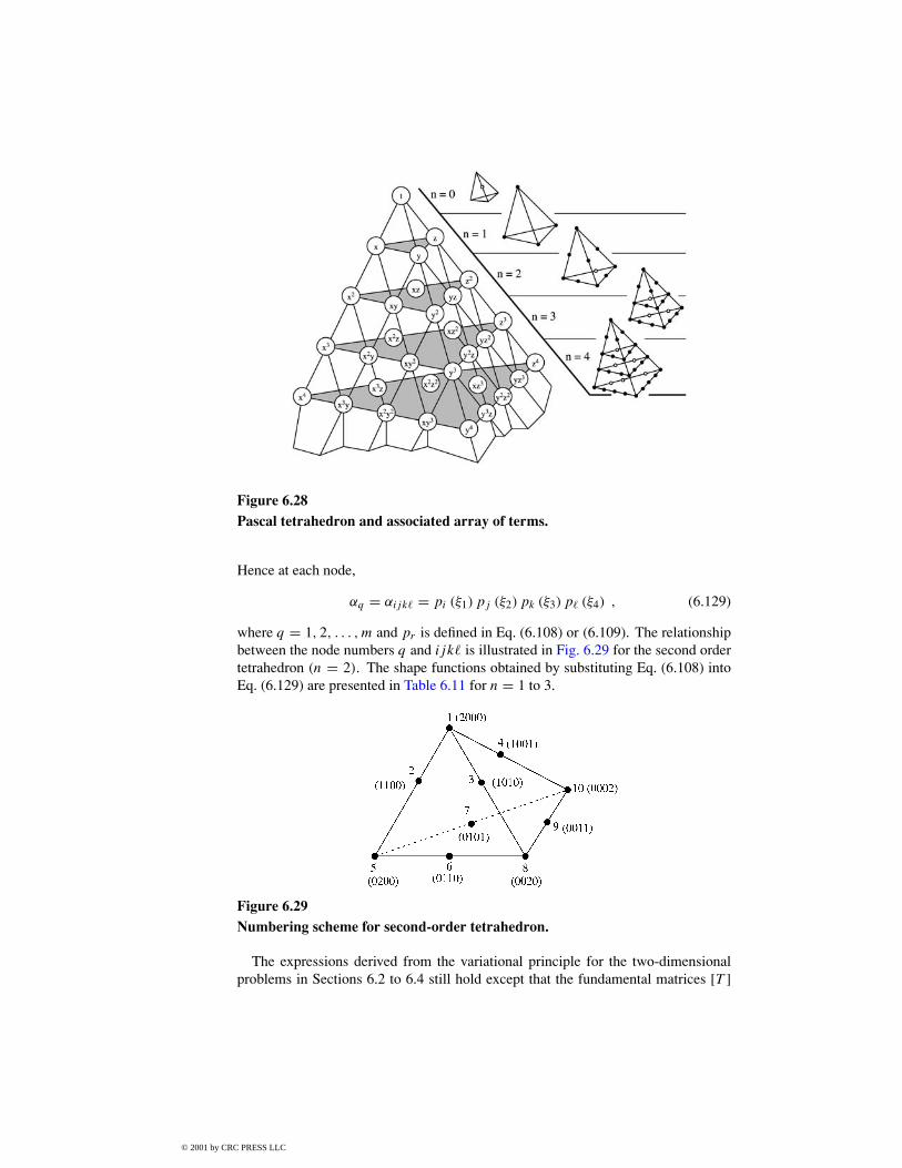
Each point in the tetrahedral element is represented by four integers i, j, k, and �which can be used to determine the local coordinates (ξ1, ξ2, ξ3, ξ4). That is at Pijk�,
where q = 1, 2, . . . , m and pr is defined in Eq. (6.108) or (6.109). The relationshipbetween the node numbers q and ijk� is illustrated in Fig. 6.29 for the second ordertetrahedron (n = 2). The shape functions obtained by substituting Eq. (6.108) intoEq. (6.129) are presented in Table 6.11 for n = 1 to 3.
Figure 6.29Numbering scheme for second-order tetrahedron.
The expressions derived from the variational principle for the two-dimensionalproblems in Sections 6.2 to 6.4 still hold except that the fundamental matrices [T ]
and [Q] now involve triple integration. For Helmholtz equation (6.56), for example,Eq. (6.68) applies, namely, [
Cff − k2Tff
]�f = 0 (6.130)
except that
C(e)ij =
∫v
∇αi · ∇αj dv
=∫v
(∂αi
∂x
∂αj
∂x+ ∂αi∂y
∂αj
∂y+ ∂αi∂z
∂αj
∂z
)dv , (6.131)
T(e)ij =
∫v
αiαj dv = v∫∫∫
αiαj dξ1 dξ2 dξ3 (6.132)
For further discussion on three-dimensional elements, one should consult Silvesterand Ferrari [4]. Applications of three-dimensional elements to EM-related problemscan be found in [49]–[53].
6.10 Finite Element Methods for Exterior Problems
Thus far in this chapter, the FEM has been presented for solving interior problems.To apply the FEM to exterior or unbounded problems such as open-type transmissionlines (e.g., microstrip), scattering, and radiation problems poses certain difficulties.To overcome these difficulties, several approaches [54]–[82] have been proposed, allof which have strengths and weaknesses. We will consider three common approaches:the infinite element method, the boundary element method, and absorbing boundarycondition.
6.10.1 Infinite Element Method
Consider the solution region shown in Fig. 6.30(a). We divide the entire domaininto a near field (n.f.) region, which is bounded, and a far field (f.f.) region, which isunbounded. The n.f. region is divided into finite triangular elements as usual, whilethe f.f. region is divided into infinite elements. Each infinite elements shares twonodes with a finite element. Here we are mainly concerned with the infinite elements.
Consider the infinite element in Fig. 6.30(b) with nodes 1 and 2 and radial sidesintersecting at point (xo, yo). We relate triangular polar coordinates (ρ, ξ) to theglobal Cartesian coordinates (x, y) as [62]
Figure 6.30(a) Division of solution region into finite and infinite elements; (b) typical infiniteelement.
where 1 ≤ ρ < ∞, 0 ≤ ξ ≤ 1. The potential distribution within the element isapproximated by a linear variation as
V = 1
ρ[V1(1− ξ)+ V2ξ ]
or
V =2∑i=1
αiVi (6.134)
where V1 and V2 are potentials at nodes 1 and 2 of the infinite elements, α1 and α2are the interpolation or shape functions, i.e.,
α1 = 1− ξρ
, α2 = ξ
ρ(6.135)
The infinite element is compatible with the ordinary first order finite element andsatisfies the boundary condition at infinity. With the shape functions in Eq. (6.135), wecan obtain the [C(e)] and [T (e)]matrices. We obtain solution for the exterior problemby using a standard finite element program with the [C(e)] and [T (e)] matrices of theinfinite elements added to the [C] and [T ] matrices of the n.f. region.
A comparison between the finite element method (FEM) and the method of mo-ments (MOM) is shown in Table 6.12. From the table, it is evident that the twomethods have properties that complement each other. In view of this, hybrid methodshave been proposed. These methods allow the use of both MOM and FEM with theaim of exploiting the strong points in each method.
Table 6.12 Comparison Between Method of Moments andFinite Element Method [83]
Method of Moments Finite Element Method
Conceptually easy Conceptually involvedRequires problem-dependent Avoids difficulties associated with
Green’s functions singularity of Green’s functionsFew equations;O(n) for 2-D, Many equations;O(n2) for 2-D,O(n2) for 3-D O(n3) for 3-D
Only boundary is discretized Entire domain is discretizedOpen boundary easy Open boundary difficultFields by integration Fields by differentiationGood representation of Good representation of
One of these hybrid methods is the so-called boundary element method (BEM).It is a finite element approach for handling exterior problems [68]–[80]. It basicallyinvolves obtaining the integral equation formulation of the boundary value prob-lem [84], and solving this by a discretization procedure similar to that used in regularfinite element analysis. Since the BEM is based on the boundary integral equivalentto the governing differential equation, only the surface of the problem domain needsto be modeled. Thus the dimension of the problem is reduced by one as in MOM. For2-D problems, the boundary elements are taken to be straight line segments, whereasfor 3-D problems, they are taken as triangular elements. Thus the shape or interpola-tion functions corresponding to subsectional bases in the MOM are used in the finiteelement analysis.
6.10.3 Absorbing Boundary Conditions
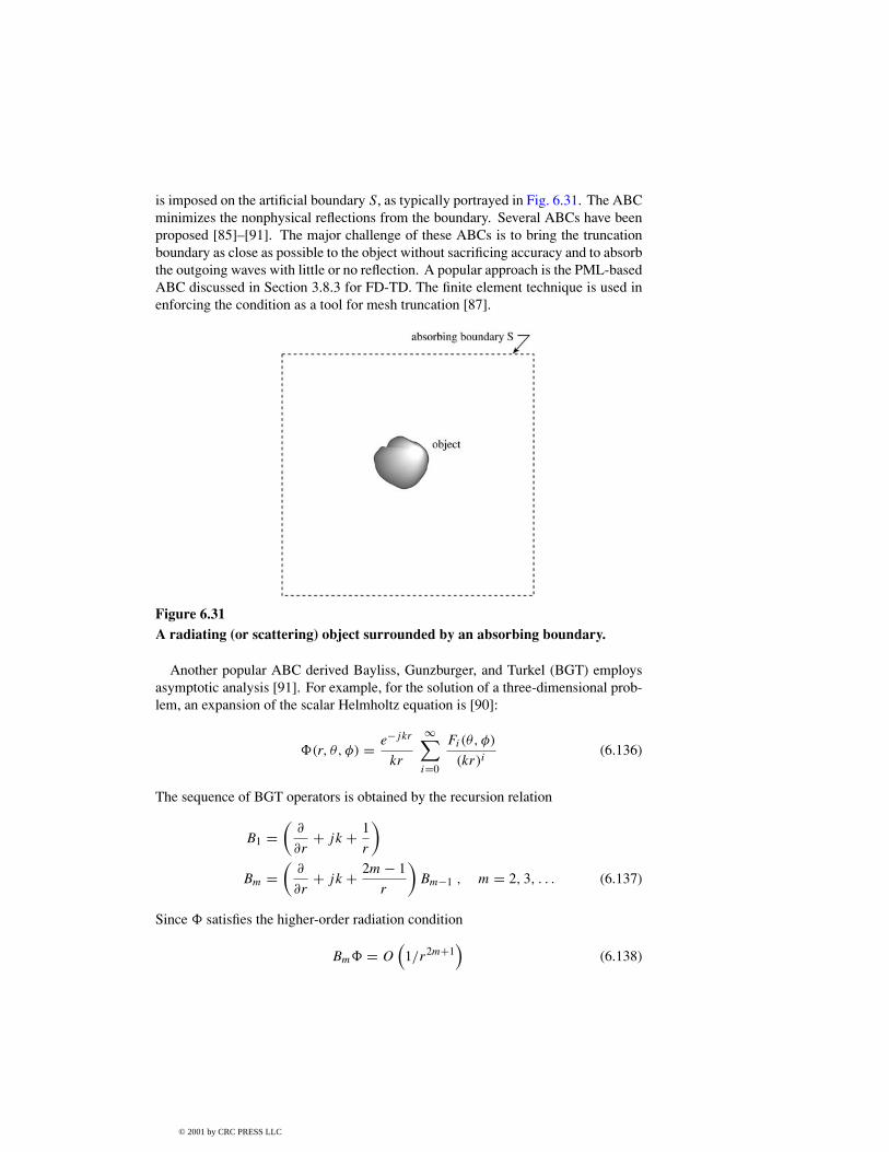
To apply the finite element approach to open region problems such as for scatteringor radiation, an artificial boundary is introduced in order to bound the region and limitthe number of unknowns to a manageable size. One would expect that as the boundaryapproaches infinity, the approximate solution tends to the exact one. But the closer theboundary to the radiating or scattering object, the less computer memory is required.To avoid the error caused by this truncation, an absorbing boundary condition (ABC)
is imposed on the artificial boundary S, as typically portrayed in Fig. 6.31. The ABCminimizes the nonphysical reflections from the boundary. Several ABCs have beenproposed [85]–[91]. The major challenge of these ABCs is to bring the truncationboundary as close as possible to the object without sacrificing accuracy and to absorbthe outgoing waves with little or no reflection. A popular approach is the PML-basedABC discussed in Section 3.8.3 for FD-TD. The finite element technique is used inenforcing the condition as a tool for mesh truncation [87].
Figure 6.31A radiating (or scattering) object surrounded by an absorbing boundary.
Another popular ABC derived Bayliss, Gunzburger, and Turkel (BGT) employsasymptotic analysis [91]. For example, for the solution of a three-dimensional prob-lem, an expansion of the scalar Helmholtz equation is [90]:
�(r, θ, φ) = e−jkr
kr
∞∑i=0
Fi(θ, φ)
(kr)i(6.136)
The sequence of BGT operators is obtained by the recursion relation
B1 =(∂
∂r+ jk + 1
r
)
Bm =(∂
∂r+ jk + 2m− 1
r
)Bm−1 , m = 2, 3, . . . (6.137)
Since � satisfies the higher-order radiation condition
will compel the solution� to match the first 2m terms of the expansion in Eq. (6.136).Equation (6.139) along with other appropriate equations is solved for�using the finiteelement method.
6.11 Concluding Remarks
An introduction to the basic concepts and applications of the finite element methodhas been presented. It is by no means an exhaustive exposition of the subject. How-ever, we have given the flavor of the way in which the ideas may be developed; theinterested reader may build on this by consulting the references. Several introductorytexts have been published on FEM. Although most of these texts are written for civil ormechanical engineers, the texts by Silvester and Ferrari [4], Chari and Silvester [41],Steele [92], Hoole [93], and Itoh [94] are for electrical engineers.
Due to its flexibility and versatility, the finite element method has become apowerful tool throughout engineering disciplines. It has been applied with greatsuccess to numerous EM-related problems. Such applications are:
• transmission line problems [95]–[97],
• optical and microwave waveguide problems [8]–[17], [92]–[103],
• electric machines [41], [104]–[106],
• scattering problems [71, 72, 75, 107, 108],
• human exposition to EM radiation [109]–[112], and
• others [113]–[116].
Applications of the FEM to time-dependent phenomena can be found in [108],[117]–[126].
For other issues on FEM not covered in this chapter, one is referred to introductorytexts on FEM such as [2, 4, 36, 41, 47], [92]–[94], [126]–[133]. The issue of edgeelements and absorbing boundary are covered in [126]. Estimating error in finiteelement solution is discussed in [52, 124, 125]. The reader may benefit from thenumerous finite element codes that are commercially available. An extensive de-scription of these systems and their capabilities can be found in [127, 134]. Althoughthe codes were developed for one field of engineering or the other, they can be appliedto problems in a different field with little or no modification.
[1] R. Courant, “Variational methods for the solution of problems of equilibriumand vibrations,” Bull. Am. Math. Soc., vol. 49, 1943, pp. 1–23.
[2] C.S. Desai and J.F. Abel, Introduction to the Finite Element Method: A Numer-ical Approach for Engineering Analysis. New York: Van Nostrand Reinhold,1972.
[3] M.N.O. Sadiku, “A simple introduction to finite element analysis of electro-magnetic problems,” IEEE Trans. Educ., vol. 32, no. 2, May 1989, pp. 85–93.
[4] P.P. Silvester and R.L. Ferrari, Finite Elements for Electrical Engineers. Cam-bridge: Cambridge University Press, 3rd ed., 1996.
[5] O.W. Andersen, “Laplacian electrostatic field calculations by finite elementswith automatic grid generation,” IEEE Trans. Power App. Syst., vol. PAS-92,no. 5, Sept./Oct. 1973, pp. 1485–1492.
[6] S. Nakamura, Computational Methods in Engineering and Science. New York:John Wiley, 1977, pp. 446, 447.
[13] M. Koshiba, et al., “Improved finite-element formulation in terms of the mag-netic field vector for dielectric waveguides,” IEEE Trans. Micro. Theo. Tech.,vol. MTT-33, no. 3, March 1985, pp. 227–233.
[14] M. Koshiba, et al., “Finite-element formulation in terms of the electric-fieldvector for electromagnetic waveguide problems,” IEEE Trans. Micro. Theo.Tech., vol. MTT-33, no. 10, Oct. 1985, pp. 900–905.
[15] K. Hayata, et al., “Vectorial finite-element method without any spurious so-lutions for dielectric waveguiding problems using transverse magnetic-fieldcomponent,” IEEE Trans. Micro. Theo. Tech., vol. MTT-34, no. 11, Nov. 1986.
[16] K. Hayata, et al., “Novel finite-element formulation without any spurious so-lutions for dielectric waveguides,” Elect. Lett., vol. 22, no. 6, March 1986,pp. 295, 296.
[17] S. Dervain, “Finite element analysis of inhomogeneous waveguides,” Mastersthesis, Department of Electrical and Computer Engineering, Florida AtlanticUniversity, Boca Raton, April 1987.
[18] J.R. Winkler and J.B. Davies, “Elimination of spurious modes in finite elementanalysis,” J. Comp. Phys., vol. 56, no. 1, Oct. 1984, pp. 1–14.
[19] M.N.O. Sadiku, et al., “A further introduction to finite element analysis ofelectromagnetic problems,” IEEE Trans. Educ., vol. 34, no. 4, Nov. 1991,pp. 322–329.
[20] The IMSL Libraries: Problem-solving software systems for numerical FOR-TRAN programming, IMSL, Houston, TX, 1984.
[21] M. Kono, “A generalized automatic mesh generation scheme for finite elementmethod,” Inter. J. Num. Method Engr., vol. 15, 1980, pp. 713–731.
[22] J.C. Cavendish, “Automatic triangulation of arbitrary planar domains for thefinite element method,” Inter. J. Num. Meth. Engr., vol. 8, 1974, pp. 676–696.
[23] A.O. Moscardini, et al., “AGTHOM—Automatic generation of triangular andhigher order meshes,” Inter. J. Num. Meth. Engr., vol. 19, 1983, pp. 1331–1353.
[24] C.O. Frederick, et al., “Two-dimensional automatic mesh generation for struc-tured analysis,” Inter. J. Num. Meth. Engr., vol. 2, no. 1, 1970, pp. 133–144.
[25] E.A. Heighway, “A mesh generation for automatically subdividing irregularpolygon into quadrilaterals,” IEEE Trans. Mag., vol. MAG-19, no. 6, Nov.1983, pp. 2535–2538.
[26] C. Kleinstreuer and J.T. Holdeman, “A triangular finite element mesh generatorfor fluid dynamic systems of arbitrary geometry,” Inter. J. Num. Meth. Engr.,vol. 15, 1980, pp. 1325–1334.
[27] A. Bykat, “Automatic generation of triangular grid I—subdivision of a generalpolygon into convex subregions. II—Triangulation of convex polygons,” Inter.J. Num. Meth. Engr., vol. 10, 1976, pp. 1329–1342.
[28] N.V. Phai, “Automatic mesh generator with tetrahedron elements,” Inter. J.Num. Meth. Engr., vol. 18, 1982, pp. 273–289.
[29] F.A. Akyuz, “Natural coordinates systems—an automatic input data generationscheme for a finite element method,” Nuclear Engr. Design, vol. 11, 1970,pp. 195–207.
[30] P. Girdinio, et al., “New developments of grid optimization by the grid iterationmethod,” in Z.J. Csendes (ed.), Computational Electromagnetism. New York:North-Holland, 1986, pp. 3–12.
[31] M. Yokoyama, “Automated computer simulation of two-dimensional elastro-static problems by finite element method,” Inter. J. Num. Meth. Engr., vol. 21,1985, pp. 2273–2287.
[32] G.F. Carey, “A mesh-refinement scheme for finite element computations,”Comp. Meth. Appl. Mech. Engr., vol. 7, 1976, pp. 93–105.
[33] K. Preiss, “Checking the topological consistency of a finite element mesh,”Inter. J. Meth. Engr., vol. 14, 1979, pp. 1805–1812.
[34] H. Kardestuncer (ed.), Finite Element Handbook. New York: McGraw-Hill,1987, pp. 4.191–4.207.
[35] W.C. Thacker, “A brief review of techniques for generating irregular compu-tational grids,” Inter. J. Num. Meth. Engr., vol. 15, 1980, pp. 1335–1341.
[36] E. Hinton and D.R.J. Owen, An Introduction to Finite Element Computations.Swansea, UK: Pineridge Press, 1979, pp. 247, 328–346.
[37] R.J. Collins, “Bandwidth reduction by automatic renumbering,” Inter. J. Num.Meth. Engr., vol. 6, 1973, pp. 345–356.
[38] E. Cuthill and J. McKee, “Reducing the bandwidth of sparse symmetric ma-trices,” ACM Nat. Conf., San Francisco, 1969, pp. 157–172.
[39] G.A. Akhras and G. Dhatt, “An automatic node relabelling scheme for min-imizing a matrix or network bandwidth,” Inter. J. Num. Meth. Engr., vol. 10,1976, pp. 787–797.
[40] F.A. Akyuz and S. Utku, “An automatic node-relabelling scheme for bandwidthminimization of stiffness matrices,” J. Amer. Inst. Aero. Astro., vol. 6, no. 4,1968, pp. 728–730.
[41] M.V.K. Chari and P.P. Silvester (eds.), Finite Elements for Electrical and Mag-netic Field Problems. Chichester: John Wiley, 1980, pp. 125–143.
[42] P. Silvester, “Construction of triangular finite element universal matrices,”Inter. J. Num. Meth. Engr., vol. 12, 1978, pp. 237–244.
[43] P. Silvester, “High-order polynomial triangular finite elements for potentialproblems,” Inter. J. Engr. Sci., vol. 7, 1969, pp. 849–861.
[44] G.O. Stone, “High-order finite elements for inhomogeneous acoustic guidingstructures,” IEEE Trans. Micro. Theory Tech., vol. MTT-21, no. 8, Aug. 1973,pp. 538–542.
[45] A. Konrad, “High-order triangular finite elements for electromagnetic wavesin anistropic media,” IEEE Trans. Micro. Theory Tech., vol. MTT-25, no. 5,May 1977, pp. 353–360.
[46] P. Daly, “Finite elements for field problems in cylindrical coordinates,” Inter.J. Num. Meth. Engr., vol. 6, 1973, pp. 169–178.
[47] C.A. Brebbia and J.J. Connor, Fundamentals of Finite Element Technique.London: Butterworth, 1973, pp. 114–118, 150–163, 191.
[48] M. Sadiku and L. Agba, “News rules for generating finite elements fundamen-tal matrices,” Proc. IEEE Southeastcon, 1989, pp. 797–801.
[49] R.L. Ferrari and G.L. Maile, “Three-dimensional finite element method forsolving electromagnetic problems,” Elect. Lett., vol. 14, no. 15, 1978, pp. 467,468.
[50] M. de Pourcq, “Field and power-density calculation by three-dimensional finiteelements,” IEEE Proc., vol. 130, Pt. H, no. 6, Oct. 1983, pp. 377–384.
[51] M.V.K. Chari, et al., “Finite element computation of three-dimensional elec-trostatic and magnetostatic field problems,” IEEE Trans. Mag., vol. MAG-19,no. 16, Nov. 1983, pp. 2321–2324.
[52] O.A. Mohammed, et al., “Validity of finite element formulation and solution ofthree dimensional magnetostatic problems in electrical devices with applica-tions to transformers and reactors,” IEEE Trans. Pow. App. Syst., vol. PAS-103,no. 7, July 1984, pp. 1846–1853.
[53] J.S. Savage and A.F. Peterson, “Higher-order vector finite elements for tetrahe-dral cells,” IEEE Trans. Micro. Theo. Tech., vol. 44, no. 6, June 1996, pp. 874–879.
[54] J.F. Lee and Z.J. Cendes, “Transfinite elements: a highly efficient procedurefor modeling open field problems,” Jour. Appl. Phys., vol. 61, no. 8, April1987, pp. 3913–3915.
[55] B.H. McDonald and A. Wexler, “Finite-element solution of unbounded fieldproblems,” IEEE Trans. Micro. Theo. Tech., vol. MTT-20, no. 12, Dec. 1972,pp. 841–847.
[56] P.P. Silvester, et al., “Exterior finite elements for 2-dimensional field problemswith open boundaries,” Proc. IEEE, vol. 124, no. 12, Dec. 1977, pp. 1267–1270.
[57] S. Washisu, et al., “Extension of finite-element method to unbounded fieldproblems,” Elect. Lett., vol. 15, no. 24, Nov. 1979, pp. 772–774.
[58] P. Silvester and M.S. Hsieh, “Finite-element solution of 2-dimensionalexterior-field problems,” Proc. IEEE, vol. 118, no. 12, Dec. 1971, pp. 1743–1747.
[59] Z.J. Csendes, “A note on the finite-element solution of exterior-field problems,”IEEE Trans. Micro. Theo. Tech., vol. MTT-24, no. 7, July 1976, pp. 468–473.
[60] T. Corzani, et al., “Numerical analysis of surface wave propagation using finiteand infinite elements,” Alta Frequenza, vol. 51, no. 3, June 1982, pp. 127–133.
[61] O.C. Zienkiewicz, et al., “Mapped infinite elements for exterior wave prob-lems,” Inter. J. Num. Meth. Engr., vol. 21, 1985.
[62] F. Medina, “An axisymmetric infinite element,” Int. J. Num. Meth. Engr.,vol. 17, 1981, pp. 1177–1185.
[63] S. Pissanetzky, “A simple infinite element,” Int. J. Comp. Math. Elect. Engr.,(COMPEL), vol. 3, no. 2, 1984, pp. 107–114.
[64] Z. Pantic and R. Mittra, “Quasi-TEM analysis of microwave transmission linesby the finite-element method,” IEEE Trans. Micro. Theo. Tech., vol. MTT-34,no. 11, Nov. 1986, pp. 1096–1103.
[65] K. Hayata, et al., “Self-consistent finite/infinite element scheme for unboundedguided wave problems,” IEEE Trans. Micro. Theo. Tech., vol. MTT-36, no. 3,Mar. 1988, pp. 614–616.
[66] P. Petre and L. Zombory, “Infinite elements and base functions for rotationallysymmetric electromagnetic waves,” IEEE Trans. Ant. Prog., vol. 36, no. 10,Oct. 1988, pp. 1490, 1491.
[67] Z.J. Csendes and J.F. Lee, “The transfinite element method for modelingMMIC devices,” IEEE Trans. Micro. Theo. Tech. vol. 36, no. 12, Dec. 1988,pp. 1639–1649.
[68] K.H. Lee, et al., “A hybrid three-dimensional electromagnetic modelingscheme,” Geophys., vol. 46, no. 5, May 1981, pp. 796–805.
[69] S.J. Salon and J.M. Schneider, “A hybrid finite element-boundary integralformulation of Poisson’s equation.” IEEE Trans. Mag., vol. MAG-17, no. 6,Nov. 1981, pp. 2574–2576.
[70] S.J. Salon and J. Peng, “Hybrid finite-element boundary-element solutions toaxisymmetric scalar potential problems,” in Z.J. Csendes (ed.), ComputationalElectromagnetics. New York: North-Holland/Elsevier, 1986, pp. 251–261.
[71] J.M. Lin and V.V. Liepa, “Application of hybrid finite element method forelectromagnetic scattering from coated cylinders,” IEEE Trans. Ant. Prop.,vol. 36, no. 1, Jan. 1988, pp. 50–54.
[72] J.M. Lin and V.V. Liepa, “A note on hybrid finite element method for solvingscattering problems,” IEEE Trans. Ant. Prop., vol. 36, no. 10, Oct. 1988,pp. 1486–1490.
[73] M.H. Lean and A. Wexler, “Accurate field computation with boundary elementmethod,” IEEE Trans. Mag., vol. MAG-18, no. 2, Mar. 1982, pp. 331-335.
[74] R.F. Harrington and T.K. Sarkar, “Boundary elements and the method of mo-ments,” in C.A. Brebbia, et al. (eds.), Boundary Elements. Southampton: CMLPubl., 1983, pp. 31–40.
[75] M.A. Morgan, et al., “Finite element-boundary integral formulation for elec-tromagnetic scattering,” Wave Motion, vol. 6, no. 1, 1984, pp. 91–103.
[76] S. Kagami and I. Fukai, “Application of boundary-element method to electro-magnetic field problems,” IEEE Trans. Micro. Theo. Tech., vol. 32, no. 4, Apr.1984, pp. 455–461.
[77] Y. Tanaka, et al., “A boundary-element analysis of TEM cells in three dimen-sions,” IEEE Trans. Elect. Comp., vol. EMC-28, no. 4, Nov. 1986, pp. 179–184.
[78] N. Kishi and T. Okoshi, “Proposal for a boundary-integral method withoutusing Green’s function,” IEEE Trans. Micro. Theo. Tech., vol. MTT-35, no. 10,Oct. 1987, pp. 887–892.
[79] D.B. Ingham, et al., “Boundary integral equation analysis of transmission-linesingularities,” IEEE Trans. Micro. Theo. Tech., vol. MTT-29, no. 11, Nov.1981, pp. 1240–1243.
[80] S. Washiru, et al., “An analysis of unbounded field problems by finite elementmethod,” Electr. Comm. Japan, vol. 64-B, no. 1, 1981, pp. 60–66.
[81] T. Yamabuchi and Y. Kagawa, “Finite element approach to unbounded Poissonand Helmholtz problems using hybrid-type infinite element,” Electr. Comm.Japan, Pt. I, vol. 68, no. 3, 1986, pp. 65–74.
[82] K.L. Wu and J. Litva, “Boundary element method for modelling MIC devices,”Elect. Lett., vol. 26, no. 8, April 1990, pp. 518–520.
[83] M.N.O. Sadiku and A.F. Peterson, “A comparison of numerical methods forcomputing electromagnetic fields,” Proc. of IEEE Southeastcon, April 1990,pp. 42–47.
[84] P.K. Kythe, An Introduction to Boundary Element Methods. Boca Raton, FL:CRC Press, 1995, p. 2.
[85] J.M. Jin et al., “Fictitious absorber for truncating finite element meshes inscattering,” IEEE Proc. H, vol. 139, Oct. 1992, pp. 472–476.
[86] R. Mittra and O. Ramahi, “Absorbing bounding conditions for direct solutionof partial differential equations arising in electromagnetic scattering prob-lems,” in M.A. Morgan (ed.), Finite Element and Finite Difference Methods inElectromagnetics. New York: Elsevier, 1990, pp. 133–173.
[87] U. Pekel and R. Mittra, “Absorbing boundary conditions for finite elementmesh truncation,” in T. Itoh et al. (eds.), Finite Element Software for MicrowaveEngineering. New York: John Wiley & Sons, 1996, pp. 267–312.
[88] U. Pekel and R. Mittra, “A finite element method frequency domain applicationof the perfectly matched layer (PML) concept,” Micro. Opt. Technol. Lett.,vol. 9, pp. 117–122.
[89] A. Boag and R. Mittra, “A numerical absorbing boundary condition for finitedifference and finite element analysis of open periodic structures,” IEEE Trans.Micro. Theo. Tech., vol. 43, no. 1 Jan. 1995, pp. 150–154.
[90] P.P. Silvester and G. Pelosi (eds.), Finite Elements for Wave Electromagnetics:Methods and Techniques. New York: IEEE Press, 1994, pp. 351–490.
[91] A.M. Bayliss, M. Gunzburger, and E. Turkel, “Boundary conditions for thenumerical solution of elliptic equation in exterior regions,” SIAM Jour. Appl.Math., vol. 42, 1982, pp. 430–451.
[92] C.W. Steele, Numerical Computation of Electric and Magnetic Fields. NewYork: Van Nostrand Reinhold, 1987.
[93] S.R. Hoole, Computer-aided Analysis and Design of Electromagnetic Devices.New York: Elsevier, 1989.
[94] T. Itoh (ed.), Numerical Technique for Microwave and Millimeterwave PassiveStructure. New York: John Wiley, 1989.
[95] R.L. Khan and G.I. Costache, “Finite element method applied to modelingcrosstalk problems on printed circuits boards,” IEEE Trans. Elect. Comp.,vol. 31, no. 1, Feb. 1989, pp. 5–15.
[96] P. Daly, “Upper and lower bounds to the characteristic impedance of trans-mission lines using the finite method,” Inter. J. Comp. Math. Elect. Engr.,(COMPEL), vol. 3, no. 2, 1984, pp. 65–78.
[97] A. Khebir, et al., “An absorbing boundary condition for quasi-TEM analysis ofmicrowave transmission lines via the finite element method,” J. Elect. WavesAppl., vol. 4, no. 2, 1990, pp. 145–157.
[98] N. Mabaya, et al., “Finite element analysis of optical waveguides,” IEEE Trans.Micro. Theo. Tech., vol. MTT-29, no. 6, June 1981, pp. 600–605.
[99] M. Ikeuchi, et al., “Analysis of open-type dielectric waveguides by the finite-element iterative method,” IEEE Trans. Micro. Theo. Tech., vol. MTT-29, no. 3,Mar. 1981, pp. 234–239.
[100] C. Yeh, et al., “Single model optical waveguides,” Appl. Optics, vol. 18, no. 10,May 1979, pp. 1490–1504.
[101] J. Katz, “Novel solution of 2-D waveguides using the finite element method,”Appl. Optics, vol. 21, no. 15, Aug. 1982, pp. 2747–2750.
[102] B.A. Rahman and J.B. Davies, “Finite-element analysis of optical and mi-crowave waveguide problems,” IEEE Trans. Micro. Theo. Tech., vol. MTT-32,no. 1, Jan. 1984, pp. 20–28.
[103] X.Q. Sheng and S. Xu, “An efficient high-order mixed-edge rectangular-element method for lossy anisotropic dielectric waveguide,” IEEE Micro. Theo.Tech., vol. 45, no. 7, July 1997, pp. 1009–1013.
[104] C.B. Rajanathan, et al., “Finite-element analysis of the Xi-core leviator,” IEEEProc., vol. 131, Pt. A, no. 1, Jan. 1984, pp. 62–66.
[105] T.L. Ma and J.D. Lavers, “A finite-element package for the analysis of elec-tromagnetic forces and power in an electric smelting furnace,” IEEE Trans.Indus. Appl., vol. IA-22, no. 4, July/Aug. 1986, pp. 578–585.
[106] C.O. Obiozor and M.N.O. Sadiku, “Finite element analysis of a solid rotorinduction motor under stator winding effects,” Proc. IEEE Southeastcon, 1991,pp. 449–453.
[107] J.L. Mason and W.J. Anderson, “Finite element solution for electromagneticscattering from two-dimensional bodies,” Inter. J. Num. Meth. Engr., vol. 21,1985, pp. 909–928.
[108] A.C. Cangellaris, et al., “Point-matching time domain finite element meth-ods for electromagnetic radiation and scattering,” IEEE Trans. Ant. Prop.,vol. AP35, 1987, pp. 1160–1173.
[109] A. Chiba, et al., “Application of finite element method to analysis of inducedcurrent densities inside human model exposed to 60 Hz electric field,” IEEETrans. Power App. Sys., vol. PAS-103, no. 7, July 1984, pp. 1895–1902.
[110] Y. Yamashita and T. Takahashi, “Use of the finite element method to determineepicardial from body surface potentials under a realistic torso model,” IEEETrans. Biomed. Engr., vol. BME-31, no. 9, Sept. 1984, pp. 611–621.
[111] M.A. Morgan, “Finite element calculation of microwave absorption by thecranial structure,” IEEE Trans. Biomed. Engr., vol. BME-28, no. 10, Oct.1981, pp. 687–695.
[112] D.R. Lynch, et al., “Finite element solution of Maxwell’s equation for hyper-thermia treatment planning,” J. Comp. Phys. vol. 58, 1985, pp. 246–269.
[113] J.R. Brauer, et al., “Dynamic electric fields computed by finite elements,” IEEETrans. Ind. Appl., vol. 25, no. 6, Nov./Dec. 1989, pp. 1088–1092.
[114] C.H. Chen and C.D. Lien, “A finite element solution of the wave propaga-tion problem for an inhomogeneous dielectric slab,” IEEE Trans. Ant. Prop.,vol. AP-27, no. 6, Nov. 1979, pp. 877–880.
[115] T.L.W. Ma and J.D. Lavers, “A finite-element package for the analysis ofelectromagnetic forces and power in an electric smelting furnace,” IEEE Trans.Ind. Appl., vol. IA-22, no. 4, July/Aug., 1986, pp. 578–585.
[116] M.A. Kolbehdari and M.N.O. Sadiku, “Finite element analysis of an arrayof rods or rectangular bars between ground,” Jour. Franklin Inst., vol. 335B,no. 1, 1998, pp. 97–107.
[117] V. Shanka, “A time-domain, finite-volume treatment for Maxwell’s equations,”Electromagnetics, vol. 10, 1990, pp. 127–145.
[118] J.H. Argyris and D.W. Scharpf, “Finite elements in time and space,” Nucl.Engr. Space Des., vol. 10, no. 4, 1969, pp. 456–464.
[119] I. Fried,“Finite-element analysis of time-dependent phenomena,” AIAA J.,vol. 7, no. 6, 1969, pp. 1170–1173.
[120] O.C. Zienkiewicz and C.J. Pareth, “Transient field problems: two-dimensionaland three-dimensional analysis by isoparametric finite elements,” Inter. J. Num.Meth. Engr., vol. 2, 1970, pp. 61–71.
[121] J.H. Argyris and A.S.L. Chan, “Applications of finite elements in space andtime,” Ingenieur-Archiv, vol. 41, 1972, pp. 235–257.
[122] J.C. Bruch and G. Zyvoloski, “Transient two-dimensional heat conductionproblems solved by the finite element method,” Inter. J. Num. Meth. Engr.,vol. 8, 1974, pp. 481–494.
[123] B. Swartz and B. Wendroff, “The relative efficiency of finite difference andfinite element methods I: hyperbolic problems and splines,” SIAM J. Numer.Anal., vol. 11, no. 5, Oct. 1974.
[124] J. Cushman, “Difference schemes or element schemes,” Int. J. Num. Meth.Engr., vol. 14, 1979, pp. 1643–1651.
[125] A.J. Baker and M.O. Soliman, “Utility of a finite element solution algorithmfor initial-value problems,” J. Comp. Phys., vol. 32, 1979, pp. 289–324.
[126] J.N. Reddy, An Introduction to the Finite Element Method. New York:McGraw-Hill, 2nd ed., 1993, pp. 293–403.
[127] C.A. Brebbia (ed.), Applied Numerical Modelling. New York: John Wiley,1978, pp. 571–586.
[128] C.A. Brebbia (ed.), Finite Element Systems: A Handbook. Berlin: Springer-Verlag, 1985.
[129] O.C. Zienkiewicz, The Finite Element Method. New York: McGraw-Hill,1977.
[130] A.J. Davies, The Finite Element Method: A First Approach. Oxford: Claren-don, 1980.
[131] C. Martin and G.F. Carey, Introduction to Finite Element Analysis: Theoryand Application. New York: McGraw-Hill, 1973.
[132] T.J. Chung, Finite Element Analysis in Fluid Dynamics. New York: McGraw-Hill, 1978.
[133] D.H. Norris and G de. Vries, An Introduction to Finite Element Analysis. NewYork: Academic Press, 1978.
[134] T. Itoh et al. (eds.), Finite Element Software for Microwave Engineering. NewYork: John Wiley & Sons, 1996.
[135] J.L. Volakis et al., Finite Element Method for Electromagnetics. New York:IEEE Press, 1998.
[136] G.R. Buchanan, Finite Element Analysis (Schaum’s Outline). New York:McGraw-Hill, 2nd ed., 1995.
[137] J. Jin, The Finite Element Method in Electromagnetics. New York: John Wiley& Sons, 1993.
[138] R. Thatcher, “Assessing the error in a finite element solution,” IEEE Trans.Micro. Theo. Tech., vol. MTT-30, no. 6, June 1982, pp. 911–914.
[139] J. Penman and M. Grieve, “Self-adaptive finite-element techniques for thecomputation of inhomogeneous Poissonian fields,” IEEE Trans. Micro. Theo.Tech., vol. 24, no. 6, Nov./Dec. 1998, pp. 1042–1049.
Problems
6.1 For the triangular elements in Fig. 6.32, determine the element coefficientmatrices.
Figure 6.32For Problem 6.1.
6.2 Find the coefficient matrix for the two-element mesh of Fig. 6.33. Given thatV2 = 10 and V4 = −10, determine V1 and V3.
6.3 Determine the shape functions α1, α2, and α3 for the element in Fig. 6.34.
6.4 Consider the mesh shown in Fig. 6.35. The shaded region is conducting andhas no finite elements. Calculate the global elements C3,10 and C3,3.
6.5 With reference to the finite element in Fig. 6.36, calculate the energy per unitlength associated with the element.
6.6 Consider the element whose sides are parallel to the x and y axis, as shownin Fig. 6.37. Verify that the potential distribution within the elements can beexpressed as
V (x, y) = α1V1 + α2V2 + α3V3 + α4V4
whereVi are the nodal potentials andαi are local interpolating functions definedas
α1 = (x − x2) (y − y4)
(x1 − x2) (y1 − y4)
α2 = (x − x1) (y − y3)
(x2 − x1) (y2 − y3)
α3 = (x − x4) (y − y2)
(x3 − x4) (y3 − y2)
α4 = (x − x3) (y − y1)
(x4 − x3) (y4 − y1)
6.7 The cross section of an infinitely long rectangular trough is shown in Fig. 6.38;develop a program using FEM to find the potential at the center of the crosssection. Take εr = 4.5.
6.8 Solve the problem in Example 3.3 using the finite element method.
6.9 Modify the program in Fig. 6.10 to calculate the electric field intensity E at anypoint in the solution region.
6.10 The program in Fig. 6.10 applies the iteration method to determine the potentialat the free nodes. Modify the program and use the band matrix method todetermine the potential. Test the program using the data in Example 6.2.
6.11 A grounded rectangular pipe with the cross section in Fig. 6.39 is half-filledwith hydrocarbons (ε = 2.5εo, ρo = 10−5 C/m3). Use FEM to determine thepotential along the liquid-air interface. Plot the potential versus x.
6.12 Solve the problem in Example 3.4 using the finite element method.
6.13 The cross section of an isosceles right-triangular waveguide is discretized as inFig. 6.40. Determine the first 10 TM cutoff wavelengths of the guide.
6.14 Using FEM, determine the first 10 cutoff wavelengths of a rectangular waveg-uide of cross section 2 cm by 1 cm. Compare your results with exact solution.Assume the guide is air-filled.
6.15 Use the mesh generation program in Fig. 6.16 to subdivide the solution regionsin Fig. 6.41. Subdivide into as many triangular elements as you choose.
6.19 Verify the interpolation functions for the six-node quadratic triangular element.
6.20 Using the area coordinates (ξ1, ξ2, ξ3) for the triangular element in Fig. 6.3,evaluate:
(a)∫Sx dS,
(b)∫Sx dS,
(c)∫Sxy dS
6.21 Evaluate the following integrals:
(a)∫Sα3
2 dS,
(b)∫Sα1α5 dS,
(c)∫Sα1α2α3 dS
6.22 Evaluate the shape functions α1, . . . , α6 for the second-order elements inFig. 6.44.
6.23 Derive matrix T for n = 2.
6.24 By hand calculation, obtain Q(2) and Q(3) for n = 1 and n = 2.
6.25 The D(q) matrix is an auxilliary matrix used along with the T matrix to deriveother fundamental matrices. An element of D is defined in [43] as the partialderivative of αi with respect to ξq evaluated at node Pj , i.e.,
D(q)ij =
∂αi
∂ξq
∣∣∣∣Pi
, i, j = 1, 2, . . . , m
where q ∈ {1, 2, 3}. For n = 1 and 2, deriveD(1). FromD(1), deriveD(2) andD(3).